1.2 ARIMA ARIMA stands for ‘Auto Regressive Integrated Moving Average’. It isactuallya model that forecastsa given time series based onthe past valuesofitsown, that is, its own forecasterrors,sowhatisusedtoforecastfuturevaluesis itsequationitself.ARIMAmodelscanbeusedforanytime series that exhibits patterns and is not random white noise. This ARIMA acronym is descriptive as it captures the important aspects of the model. These are AR, I, and MA which stand for Autoregression, Integrated, and Moving Average. Autoregression [6] refers to a model in which the dependent relationship between some lagged observations and observation is utilized. Secondly, Integrated refers to the use of subtracting raw observations in order to make the time series seem stationary.MovingAverages[7]isamodelthatputstouse the dependence between a residual error and an observation from a similar model applied to the observations which are lagged. When we combine seasonality to ARIMA, it results in the Seasonal ARIMA model[13]. The aforementioned parameters of the ARIMA model can bedescribedasfollows: ● p(autoregressive order): Lag observations’ numberincludedinthemodel.
***
Abstract This paper investigates the implementation of the models ARIMA [3] and Prophet to forecast the inconsistencies in reactive power. We propose the usage of two models for prediction and go on to analyse which works more efficiently with the help of performance metrics MSE and RMSE. We use the data received periodically from a transformer over a period of twelve months. Using the aforementioned data, we prioritise the ARIMA model over the Prophet model since it portrays highly promising results in comparison.
Key Words: ARIMA, Prophet, Time Series Forecasting, Autoregression,PowerGrid,SARIMA
1.INTRODUCTION In an electrical power grid, the power load is not consistent. The inconsistency might result from various factors like the seasons, hour of the day, and climate. The perpetual variation in energy consumption necessitates the power grid to be flexible. Transformers play a vital role in the power grid. Hence, monitoring of the transformersiscrucialtopreventthefailureofthepower grid. By monitoring the transformers continuously, the transformer's life can be improved, be utilized to their total potential, and reduce the maintenance cost. The rapidly progressing requirement for power supply adds substantial pressure on the asset owners to look after their more essential transformers. In this paper, we addressthisrequirementwiththehelpoftwoapproaches oftimeseriesforecasting.
2Student, Dept. of Computer Science and Engineering, Chaitanya Bharathi Institute of Technology, Telangana, India
Analysis of Time Series Forecasting for Reactive Power of a Transformer Sai Sanjeev Kumar Reddy Boppidi1, Sai Annanya Sree Vedala2
International Research Journal of Engineering and Technology (IRJET) e ISSN: 2395 0056 Volume: 08 Issue: 11 | Nov 2021 www.irjet.net p ISSN: 2395 0072 © 2021, IRJET | Impact Factor value: 7.529 | ISO 9001:2008 Certified Journal | Page1577
1.1 Time Series Forecasting A time series [2][9] is essentially a sequence where a metric is recorded over periodic time intervals. A time series can be yearly, quarterly, monthly, weekly, daily, hourly, and even seconds wise, depending on how often the data is obtained. An example of a yearly time series wouldbeanannual budget anda secondwise timeseries wouldbethatofwebtraffic.Timeseries forecasting[1]is where we want to predict the future values that a time series is likely to take. Forecasting a time series, for instance,demandandsalesbecomeshighlyessentialsince it associates with a tremendous commercial value. In many companies belonging to sectors like manufacturing, finance,realestate,etc.,itdrivesthefundamentalbusiness planning, procurement, and management activities. Any errorsintheforecastswouldbeveryexpensivesincethey would affect the entire supply chain. It is thus highly important to get accurate predictions to not end up in losses.Time series forecasting is divided into two umbrellas. These are Univariate Time Series Forecasting [4] and Multivariate Time Series Forecasting [5]. If only the previous values of the time series are utilized to predict thenextvalues,itisUnivariateTimeSeriesForecasting.If otherpredictorsareusedotherthanthepreviousvalueof the series or the series itself to make predictions, it is Multivariate Time Series Forecasting. Forecasting and prediction sometimes are used interchangeably, however, there is a notable distinction. In some fields, data at a specific future point in time can be referred to as forecasting, future data in general is referred to as prediction.Seriesforecastingisoftenusedalongwithtime series analysis. Time series analysis includes the development of models to attain an understanding of the datatounderstandtheunderlyingtrends.
1Student, Dept. of Computer Science and Engineering, Chaitanya Bharathi Institute of Technology, Telangana, India

1.3 Prophet Prophet is an open source tool developed by Facebook which utilizes a Bayesian based curve fitting method to forecast the time series data. In Prophet, trends are fit with yearly, weekly, and daily seasonality, and holiday effects. It uses Fourier series and a weekly seasonal component modeled using dummy variables to include a yearly seasonal component. It is an entirely automated procedure that enables users to develop forecasts quickly and easily. The Prophet procedure provides users with manypossibilitiestotweakandmodifyforecasts.Prophet works most efficiently time series with strong seasonal data and a considerable number of seasons of historical data
Mehdi Khashei et al. [17], compare performance for the ANN, SARIMA, and Fuzzy logic models both individually and in combinations. Their results show that it is often better to combine different models than to just go with one model. Many other models in combination make up forthefactthatSARIMAdoesnotfavornon lineardata.A set of previous data is required for the SARIMA and ARIMA models, which is not often available in the real world.Usually,thedataavailableisless,ARIMAmightnot bethebestuseforsuchaforecast.
The field of time series forecasting has been used for multipledifferenttasksthatrequireplanningoftendueto restrictions in adaptability. ARIMA is a very popular algorithmfortimeseriesforecasting.ARIMAmodelswere introduced in the 1950s initially but were popularised by George E. P. Box as well as Gwilym Jenkins. To get a clear overview of what ARIMA is, we must first break it down into smaller pieces. An Autoregressive model (AR) representsarandomprocess.Intheautoregressivemodel, the output depends on previous inputs and a stochastic term. AR models take past steps into consideration when calculating the next step. The issue with the AR model is that temporary or single shocks affect the whole output indefinitely. To avoid this, lag values exist. The lag value refers to the number of the previous steps that should be usedtocontributetotheoutputmoreextensivelythanthe others. The AR model can be non stationary as it can be represented by a unit root variable. The MA (Moving Average) model, however, is always stationary. Moving averageisalinearregressionmodelconsideringtheshock values, contrary to the AR model which is the linear regression to non shock values. There is no reason why you cannot combine these models and that is where the ARMA process comes in. The ARMA model combines the twomodelstomakeanaccurateprediction whichismore thantheexistingaccuracy.TheARMAmodelcomparesthe results for both models and makes a prediction based on the results [18]. The drawback of the ARMA process is it assumes a stationary time series. Thus it will not take seasonality into account. That is where ARIMA comes in handy. The I in ARIMA stands for integrated, which is the subtracting of previous observations in the series. Non
International Research Journal of Engineering and Technology (IRJET) e ISSN: 2395 0056 Volume: 08 Issue: 11 | Nov 2021 www.irjet.net p ISSN: 2395 0072 © 2021, IRJET | Impact Factor value: 7.529 | ISO 9001:2008 Certified Journal | Page1578
● d(differencing order): Count of the times the raw observationsaresubtracted. ● q(moving average order): The size of the moving averagewindow. A linear regression [8] model generally includes a specified number and type of terms. The data is further prepared with the help of a degree of differencing to remove trend and seasonal structures that are unfavourable ie., make it stationary. 0 is often used for a parameter whichshould not be usedas an element of the model.Inthismanner,ARIMAmodelscanbeconfiguredto perform the function of an ARMA model, an AR, I, or MA model as well. When an ARIMA model is used for a time series forecasting, it is assumed that the process that generated the observations in the first place is an ARIMA process. This helps to motivate the requirement to assert theassumptionsofthemodelintherawobservationsand residualerrorsofforecasts.
2. LITERATURE SURVEY Weinvestigatedtwoofthemostsignificantdatabases,the IEEE and ACM databases. We looked for the term "time series forecasting" and found similar forecasting methods in most articles and reports. In the process of our literature survey, we did not specify "time series forecasting for a smart grid" since we wished to perform moregeneralbasedsearchandgetabirds eyeviewofthe fieldoftimeseriesforecasting.Wewillusethissurveyand the documents as the base for our methodology and progress. We have decided to separate the method into three groups. Machine learning, ARIMA, and other techniques. In a report from 2012, Mehdi Khashei and MehdiBijari[15],proposedahybridofanArtificialNeural Network and ARIMA model to overcome some of the limitationsoftheARIMAmodels.3differentdatasetswith different characteristics were used to test the model. According to them, ARIMA models generally tend to have low accuracy for predicting non linear data. They observed that their hybrid solution outperformed the results that came when the models were separately implemented. The Mean Absolute Error (MAE) and Mean SquaredError(MSE)fortheshortaswellasthelong term forecasting showed better results with the hybrid model.
2.1 ARIMA Models Related Work
Bangzhu Zhu and Yiming Wei [16] suggested a hybrid model that uses a Least Squared Vector Model with the ARIMA models, which is a neural network model used to forecast the prices of carbon in the EU. Three different kinds of hybrid models are proposed that were implemented on a dataset that is non stationary and the results show a clear advantage of combining the models.
2.2 Other Techniques
There are multiple different techniques used for time series forecasting, but the two previously mentioned methodsarebyfarthemorepopularoptionstoday.There are different mathematical models that can be used for forecasting such as state space models. The idea of space statemodelsisthatanydynamicsystemcanbedefinedby differentialequations.Thismeansthatthecurrentstateof the system is defined by the previous state and a state variable that changed the state. By this observation, we can define any system as a function of its states and externalinputs.Byknowingsomeoftheobserveddata,we can calculate the optimal estimation for a selected state. TheARIMAmodelscanalsobeconvertedintospacestate models [19], as they are to some degree differential equations as well. There are many variations on SSM but the mostused isthelinear SSM[19]. Other workstend to use a combination of models to create hybrid models to eliminate the inherent flaws of some models [20] and many of the works compare their hybrid solution to the preexisting models. A study from 2013 uses an Exponential Smoothing Space State model comparing it with other algorithms to forecast solar irradiance. The used data set had data collected monthly and the Kwiatkowski Phillips Schmidt Shin (KPSS) stationary test proved the time series to be non stationary. The results concluded that the ESSS model out performed ARIMA, LinearExponentialSmoothing,andSimpleExponential14 smoothing except for two months, but was only 0.5% behind, which means that the ESSS is a reliable model for theirdataset.
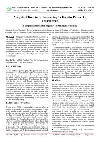
The dataset we used is recorded by IoT sensors every 15 minutes over a period of 12 months from a transmission grid in Tripura, India. The dataset consists of various parameters as described below. We worked on the parameter "Reactive Power"(KVAR) to learn the working ofTime SeriesForecastingalgorithms.
Fig -1:Snippetofthedataframewhichconsistsof7 columns. Givenaboveisasnippetofthedatathatwasusedforthis project. The dataset had 7 columns and 60134 rows. The columnsareasfollows: ● DeviceImei: TheIMEInumberofthetransformerfrom whichwearereceivingthedata.
● DeviceTimeStamp: The dataset recorded data every 15 minutes as mentioned above. The time of the data beingprocuredisrecordedanddisplayedinthiscolumn.
3. DATASET DESCRIPTION
● KVARH: KVARHstandsforKiloVoltAmperesReactive Hours. It is a unit of reactive energy consumption, most commonly used in industries. Here, this column refers to thesameunitofthetransformerevery15minutes.
International Research Journal of Engineering and Technology (IRJET) e ISSN: 2395 0056 Volume: 08 Issue: 11 | Nov 2021 www.irjet.net p ISSN: 2395 0072 © 2021, IRJET | Impact Factor value: 7.529 | ISO 9001:2008 Certified Journal | Page1579
seasonal ARIMA is often described as ARIMA (p, d, q) where p is the number of lags in the AR model, d is the gradeofdifferentiation(thenumberoftimesthedata has previous values subtracted) and the q is the order of the MA model. As the ARIMA models are a combination of models,ARIMA(1,0,0)isthesameasanAR(1)modelas the integrated part and the moving average are not used. Lag refers to the delay in steps of time between two data set points that are being compared. The order of MA is how many of the previous shocks that the model will considerwhenpredicting.Ashockisanexternalinfluence or something that changes the value to an extreme point, both high and low. In the same way any ARIMA (p, d, q) where p is 0 is equal to an ARMA (p, q) model. Lastly, we aim to investigate different machine learning techniques asmachinelearninghasbeenmoreandmoreprevalentin many areas in the last years. The concept of machine learningisnotjusttoinstructtheprogramonhowtosolve a problem, but instead to give the problem and let the computer solve it in its own way. One of the most prevalent solutions regarding machine learning and time seriesforecastingistheusageofneuralnetworks.Aneural network is a network of nodes that are connected and communicatewitheachothertosolveatask.Thenetwork has one or more layers that are not visible but have neurons. These are the nodes with the information that helpscalculatetheresultforthegivenproblem.Theresult is not a definitive result, but rather an estimated result and the accuracy of the result depends on the number of hidden "neurons" and layers in the network. The more neuronsandlayers,themorecalculations/operations,and themoreaccurateoutput.
● KW: ItstandsforKiloWatt.Itcomprises1000Watts.It isaunitofelectricpower.Itreferstothepowerdissipated bythetransformer.
● KVA: AKVArefersto1,000voltamps.Avoltisaunitof electrical pressure and an ampere is a unit of electrical current. Apparent power is the term used for the product of the volts and amps. This column contains this unit of powerofthetransformer.
● KWH: Theenergythata deviceconsumesismeasured in KWH(Kilowatt Hour). The kilowatt hour consumption recordshowmany wattsareusedandhowoftentheyare used. In our dataset, the KWH signifies the measurement ofthetransfomer’swattage and theamountoftimeitwas used.
● KVAR: It stands for Kilo Watt Amp Reactive. This unit is usually used to express power in all forms, but is most commonly used to express real power. This column describesthisunitofthetransformer.
International Research Journal of Engineering and Technology (IRJET) e ISSN: 2395 0056 Volume: 08 Issue: 11 | Nov 2021 www.irjet.net p ISSN: 2395 0072 © 2021, IRJET | Impact Factor value: 7.529 | ISO 9001:2008 Certified Journal | Page1580 Given above is the description of the different columns of thedataset. Column name Unit name KWH Kilowatt hour KVARH KilovoltAmperesReactiveHours KW Kilowatt KVA KilovoltAmperes KVAR KilovoltAmperesReactive Table 1:Columnsandunits Above table gives the units of different parameters which aregiveninthedataframe 4. 4.1METHODOLOGYStationarityAnalysis Oneoftheessentialpropertiestoanalyzewhenexamining data sets or time series is the stationarity of the time series. A stationary time series [9][12] is not affected by seasonality, i.e., the trend is consistent. To evaluate the stationarity of our dataset, we adopted Augmented Dickey Fuller Test [10]. This test is based on an autoregression model, which optimizes for different lag values.Lagisthedelayintime betweentwovaluesinthe time series that you are comparing. The mathematical formulaofAugmentedDickey Fullertestcanbegivenas: α =constant β =coefficientontimetrend p =lagorderoftheautoregressiveprocess ��t =variableofinterest �� =timeindex Δ =firstdifferenceoperator The Augmented Dickey Fuller test uses a lag variable to eliminateautocorrelationfromtheresults.Supportingthe nullhypothesisthat��=0againstthealternativehypothesis ��<0,theunittestiscarriedout.InPython,theAugmented Dickey Fuller test is available in the Statsmodels package asadfuller().TheTable 2showsthecriticalvaluesforthe Dickey FullerTest. TheTable 2showsthecriticalvaluesfortheDickey Fuller Test. Sample Size 1% T=25 4.38 T=50 4.15 T=100 4.04 T=250 3.99 T=500 3.98 T=501+ 3.96 CalculatedValue: 3.705 Table -2:CriticalvaluesforAugmentedDickey FullerTest andourresultsfromtheroottest. By observing the critical values we can see that the calculated value is not lower than the critical value than the critical value, which means that we cannot reject the nullhypothesisandthetimeseriesisnotstationary. 4.2 Implementation Of ARIMA Our previous results showed that the time series is not stationary, this affects the selection of the ARIMA models. Sinceourtimeseriesshowbothseasonalityandtrend,the Seasonal ARIMA model is the best choice. H. Matsila et al. [11] used the Seasonal ARIMA model for successfully forecasting over their small data set. They had a weekly seasonality and did short forecasts with very high accuracy. Hence, we chose Seasonal ARIMA Model to weigh in the seasonality and produce results with higher accuracy. The Seasonal ARIMA model requires 7 parameters usually denoted by SARIMA (p,d,q)(P,D,Q)m, where (p,d,q)are trend order and (P,D,Q)m represent the seasonalorder. Thetrendorderisthesamevalueswhich we would be using for fitting an ARIMA model, i.e., p is autoregressive order, d is differencing order and q is moving average order as mentioned above. The seasonal elements also have the same parameters, however, m is the number of time steps for each season. We used a grid search to get the most fitting parameters for the ARIMA forecasting models. We defined a set of model combinations to test which forecast model has the lowest error regarding our data set. To evaluate which model is the best fit, we assessed based on multiple one step forecasts, compared the actual value, and calculated the RMSE.The model that thegridsearchfound outto be the best is the ARIMA(1,0,2)(2,1,0)100 with no trend, linear trend,andconstantwithalineartrend.
4.3 Implementation Of Prophet Facebook'sProphetModelhasafewlimitationsonhowits data should be represented. It presumes to have an input
To evaluate the individual forecasting models prediction ability, we made use of commonly used performance metricsformeasuringpredictionerrors.Predictionerrors are the difference between the predicted and the actual values. MSEandRMSEgivetheerrorinregardtomedian ofthedata.
International Research Journal of Engineering and Technology (IRJET) e ISSN: 2395 0056 Volume: 08 Issue: 11 | Nov 2021 www.irjet.net p ISSN: 2395 0072 © 2021, IRJET | Impact Factor value: 7.529 | ISO 9001:2008 Certified Journal | Page1581
5. PERFORMANCE METRICS
A commonly used metric for evaluating results of predictionsistheRootmeansquareerror,alsoreferredto as root mean square deviation. Similar to mean squared error, it shows how far the true values are from the predictions.RMSEusesEuclideandistancetomeasurethe distance. To calculate RMSE, we have to calculate the residualwhichisthedifferencebetweenthetruthandthe prediction for every data point. We then have to compute the residual norm at all data points, and further calculate themeanoftheseresidualstofinallytakethesquareroot of the obtained mean. RMSE needs true measurements at each predicted data point, thus, it is commonly used in supervisedlearningproblems. WecanexpressRMSEas
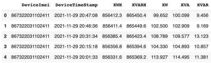
Fig -2 :VisualizationofforecastedvaluesofreactivepowerusingARIMA.
∑ ( ) Intheaboveformula, MSE =MeanSquaredError
5.2 Root Mean Squared Error
√∑ ( ) RMSEwhere, =RootMeanSquaredError n =Numberofdatapoints xi =ActualValues xi ’ =PredictedValues
of two columns, namely ‘ds’ for Date Time Stamp and ‘y’ for target variable. The model does not accept any other names for columns. In our data the target variable is ‘KVAR’. A Prophet() object is defined and configured in order to use Prophet for forecasting. Then it is fit on the dataset by calling fit() function and passing the data to it. The Prophet() object takes seasonalityasanargument. In ourcase,wetooktheseasonalitytobeweekly.Themodel figuresoutalmosteverythingelseautomatically. By calling the predict() function and passing the data frame that contains the column named ‘ds’ and all the rows with date times for which the forecasts are to be made. The result of the predict() function is a data frame which consists of numerous columns, out of which the most important are the columns ‘ds’ and ‘yhat’, where ‘yhat’isthepredictedvalue.Thecolumns‘yhat_upper’and ‘yhat_lower’ give the uncertainty of the forecasted value. The forecasted values can be visualized with the help of plot().
n =Numberofdatapoints xi =ActualValues x’ =PredictedValues
5.1 Mean Squared Error
The mean squared error is a measure that refers to how closea setof pointsis tothestructuredregressionline. It is measured by calculating the distances from each of the points to the regression line and squaring them. These distances are essentially the errors. The squaring of the distance is done to remove the negative values. It gives higher importance and weight to larger differences. Since weare finding theaverage ofa set of errors,itisreferred toasthemeansquarederror.WepreferalowerMSE,this signifiesabetterforecast.
[5] Chakraborty, K., Mehrotra, K., Mohan, C., & Ranka, S. (1992). Forecasting the behavior of multivariate time seriesusingneuralnetworks. [6] Hannan, E., & Kavalieris, L. (1986). REGRESSION, AUTOREGRESSION MODELS. Journal Of Time Series Analysis [7] "GeneralizedAutoregressiveMovingAverageModels". 2021.JournalOfTheAmericanStatisticalAssociation. [8] "Applied Linear Regression". 2021. Google OOjcC&oi=fndhttps://books.google.co.in/books?hl=en&lr=&id=xd0tNdFBooks.
[4] Moritz, S. et al. (2015) Comparison of different Methods for Univariate Time Series Imputation in R, arXiv.org.Availableat:https://arxiv.org/abs/1510.03924
[10] W. A. Dickey, D. A.; Fuller, “Distribution of the estimatorsforautoregressivetimeserieswithaunitroot,” Journal of the American Statistical Association, vol. 74, p. 427 431,1979.
[11] H. Matsila and P. Bokoro, “Load Forecasting Using Statistical Time Series Model in a Medium Voltage Distribution Network,” in IECON 2018 44th Annual
[9] ndForecasting,3rded.P.J.BrockwellandR.A.Davis,IntroductiontoTimeSeriesaSpringer,2016.
REFERENCES
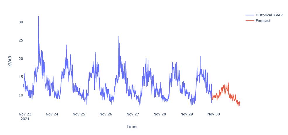
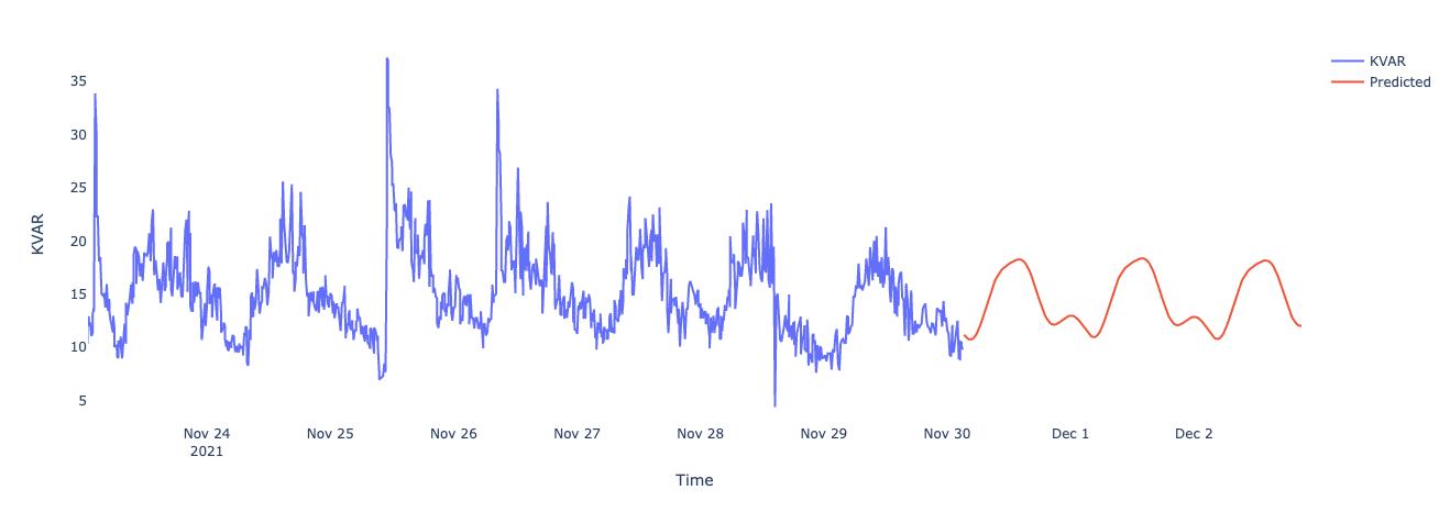
International Research Journal of Engineering and Technology (IRJET) e ISSN: 2395 0056 Volume: 08 Issue: 11 | Nov 2021 www.irjet.net p ISSN: 2395 0072 © 2021, IRJET | Impact Factor value: 7.529 | ISO 9001:2008 Certified Journal | Page1582 Fig 3 :VisualizationofforecastedvaluesofreactivepowerusingProphet.
6. RESULTS We analysed our data set and investigated the implementation of traditional Seasonal ARIMA and Prophet time series forecasting methods. As mentioned earlier, the difference between the real value and the estimated value of the data is found with the MSE (Mean SquareError)andRMSE(SquareRootoftheMeanSquare Error) methods. The MSE value for the forecasting using ARIMA Model is 14.006 and the RMSE value is 3.743. When we used the Prophet Model the MSE and RMSE turnedouttobe18.915and4.349respectively.
[3] Fattah, Jamal & Ezzine, Latifa & Aman, Zineb & Moussami, Haj & Lachhab, Abdeslam. (2018). Forecasting of demand using ARIMA model. International Journal of Engineering Business Management. 10. 184797901880867.10.1177/1847979018808673.
8. CONCLUSION In conclusion, we were successful in perfectly laying out the differences in the performances of the ARIMA model and the Prophet model. We also went on to explain the highly likely reasons for the same. In data of the sort that weused,ARIMAgivesthebestresultssinceitdoesn’tneed dataofaverylongtimespan.Itsuccessfullyworksondata withashorttimespantoo.
7. DISCUSSION AND FUTURE WORK Fromtheresultsgathered,inourcaseforthisdatasetand the algorithms we used, the Seasonal ARIMA model had the best prediction accuracy of the tested methods. It can be clearly observed that the ARIMA model shows best resultsasit’sappliedoverashortperiodoftime.Whereas, theProphetcouldn’tshowsatisfactoryresults. Asaprospectofthefuturework,thesamedatasetcansee the implementation of a different set of models including exponential smoothing and LSTM to check the results. Additionally, the data that was obtained from the transformer was only power related, the next step could be to apply the similar models to different sets of data obtainedinrealtimefromthetransformer.Thiscouldlead tobetterresultsoftimeseriesforecasting.
[1] D.Webby, R. and O'Connor, M.Webby, Richard, and MarcusO'Connor."JudgementalandStatisticalTimeSeries Forecasting: A Review Of The Literature". International Journal of Forecasting, vol 12, no. 1, 1996, pp. 91 118. ElsevierBV [2] BryanLimandStefanZohren"TimeSeriesForecasting With Deep Learning: A Survey(2021) Available at: https://arxiv.org/pdf/2004.13408.pdf
Conference of the IEEE Industrial Electronics Society. IEEE,2018.
[15] M. Khashei and M. Bijari, “A novel hybridization of artificialneuralnetworksandarimamodelsfortimeseries forecasting,”Expertsystemswithapplications,vol. 39,pp. 4344 4357,2012.
[18] P. J. Brockwell and R. A. Davis, Introduction to Time SeriesandForecasting,3rded.Springer,2016.
[20] G. P. Zhang, “Time series forecasting using a hybrid arima and neural network model,” Neurocomputing, vol. 50,p.159 175,2003
[14] Rougier, Jonathan. 2016. "Ensemble Averaging And Mean Squared Error". Journal Of Climate 29 (24): 8865 8870.doi:10.1175/jcli d 16 0012.1.
[19] F.D.K.S.K.V.M.J.W.W. Paninski L, Ahmadian Y, “A new look at state space models for neural data,” Journal of ComputationalNeuroscience,vol.29,pp.107 126,2006.
[12] Whittle, P. 1953. "Estimation And Information In StationaryTimeSeries".ArkivFörMatematik2. [13] Baldigara, Tea, and Maja Mamula. 2015. "Modelling International Tourism Demand Using Seasonal ARIMA Models".
International Research Journal of Engineering and Technology (IRJET) e ISSN: 2395 0056 Volume: 08 Issue: 11 | Nov 2021 www.irjet.net p ISSN: 2395 0072 © 2021, IRJET | Impact Factor value: 7.529 | ISO 9001:2008 Certified Journal | Page1583
[17] M. B. Mehdi Khashei and S. R. Hejazi, “Combining seasonal arima models with computational intelligence techniques for time series forecasting,” Soft Computing, vol.16,pp.1091 1105,2012.
[16] B. Z. . Y.Wei, “Carbon price forecasting with a novel hybrid arima and least squares support vector machines methodology,”Omega,vol.41,pp.517 524,2013.