
Advances in Applied Sciences
Advances in Applied Sciences (IJAAS) isapeer-reviewedandopenaccessjournaldedicatedtopublish significantresearchfindingsinthefieldofappliedandtheoreticalsciences.Thejournalisdesignedtoserve researchers,developers,professionals,graduatestudentsandothersinterestedinstate-of-theartresearch activitiesinappliedscienceareas,whichcovertopicsincluding:chemistry,physics,materials,nanoscience andnanotechnology,mathematics,statistics,geologyandearthsciences.
Editor-in-Chief: Qing Wang, National Institute of Advanced Industrial Science and Technology (AIST), Japan
Co-Editor-in-Chief:
Chen-Yuan Chen, National Pingtung University of Education, Taiwan, Province of China Bensafi Abd-El-Hamid, Abou BekrBelkaid University of Tlemcen, Algeria Guangming Yao, Clarkson University, United States HabibollaLatifizadeh, Shiraz (SUTECH) University, Iran, Islamic Republic of EL Mahdi Ahmed Haroun, University of Bahri, Sudan
Published by:
Institute of Advanced Engineering and Science (IAES)
Website: http://iaescore.com/journals/index.php/IJAAS/ Email: info@iaesjournal.com, IJAAS@iaesjournal.com
ISSN: 2252-8814
IJAAS
Information for Authors
International Journal of Advances in Applied Sciences (IJAAS) is an interdisciplinary journal that publishes material on all aspects of applied and theoretical sciences. The journal encompasses a variety of topics, including chemistry, physics, materials, nanoscience and nanotechnology, mathematics, statistics, geology and earth sciences.
Submission of a manuscript implies that it contains original work and has not been published or submitted for publication elsewhere. It also implies the transfer of the copyright from the author to the publisher. Authors should include permission to reproduceany previously published material.
Ethicsinpublishing
For information on Ethics in publishing and Ethical guidelines for journal publication (including the necessity to avoid plagiarism and duplicate publication) see http://www.iaescore.com/journals/index.php/IJAAS/about/editorialPolicies#sectionPolicies
PaperSubmission
You must prepareand submit your papers as word document (DOC or DOCX).
For more detailed instructions and IJAAS template please takea look and download at: http://www.iaescore.com/journals/index.php/IJAAS/about/submissions#onlineSubmissions
The manuscript will be subjected to a full review procedure and the decision whether to accept it will be taken by the Editor based on the reviews.
Manuscript must be submitted through our on-line system: http://www.iaescore.com/journals/index.php/IJAAS/
Once a manuscript has successfully been submitted via the online submission system authors may track the status of their manuscript usingthe online submission system.
International Journal of
Advances in Applied Sciences
High impedance fault detection in distribution system
KavaskarSekar,NalinKantMohanty 95-102
Frequency regulation of modern power system using novel hybrid DE-DA algorithm
SayantanSinha,RanjanKumarMallick 103-116
Enhanced performance of PID load frequency controller for power systems
DolaGobindaPadhan,SureshKumarTummala
Solar irradiance forecasting using fuzzy logic and multilinear regression approach: a case study of Punjab, India
SahilMehta,PrasenjitBasak
Solar panel monitoring and energy prediction for smart solar system
IshaM.Shirbhate,SunitaS.Barve
Performance evaluation and comparison of diode clamped multilevel inverter and hybrid inverter based on PD and APOD modulation techniques
N.Susheela,P.SatishKumar 143-153
Solar energy storage and release application of water-phase change material- (SnO2-TaC) and (SnO2–SiC) nanoparticles system
FarhanLaftaRashid,AseelHadi,AmmarAliAbid,AhmedHashim
A model free dissolved oxygen controller for industry effluent using hybrid variables measuring technique
P.KingstonStanley,SanjeeviGandhiA.,D.AbrahamChandy 157-163
Subsynchronous resonance oscillations mitigation via fuzzy controlled novel braking resistor model
MohamedFayez,M.Mandour,M.El-Hadidy,F.Bendary 164-170
Responsibility of the contents rests upon the authors and not upon the publisher or editors.
IJAAS
117-124
125-135
136-142
154-156
IJAAS Vol.8 No.2 pp.95-170 June2019 ISSN2252-8814
InternationalJournalofAdvancesinAppliedSciences(IJAAS) Vol.8,No.2, June2019,pp.95~102
ISSN:2252-8814,DOI:10.11591/ijaas.v8.i2.pp95-102
Highimpedancefaultdetectionindistributionsystem
KavaskarSekar1,NalinKantMohanty2
1DepartmentofElectricaland ElectronicsEngineering,PanimalarEngineeringCollege,India
2DepartmentofElectricalandElectronicsEngineering,SriVenkateswaraCollegeofEngineering,India
Article Info
Article history:
ReceivedAug30,2018
RevisedMar 20,2019
AcceptedApr17,2019
Keywords:
Discretewavelettransform
Highimpedancefault
Neuralnetworks
Non-linearload
Corresponding Author:
KavaskarSekar,
ABSTRACT
High impedance faults (HIFs) present a huge complexity of identification in an electric power distribution network (EPDN) due to their characteristics. Further,the growthofnon-linearload adds complexity in HIF detection.One primary challenge of power system engineers is to reliably detect and discriminate HIFs from normal distribution system load and other switching transient disturbances. In this study, a novel HIF detection method is proposed based on the simulation of an accurate model of an actual EPDN studywith realdata. Theproposed method usescurrentsignalaloneand does not require voltage signal. Wavelet transform (WT) is used for signal decomposition to extract statistical features and classification of HIF into Non-HIF (NHIF) by Neural Networks (NNs). The simulation study of the proposed methodprovidesgood,consistentandpowerfulprotection forHIF.
Copyright © 2019 Institute of Advanced Engineering and Science. All rights reserved.
DepartmentofElectricalandElectronicsEngineering, AnnaUniversity, Guindy,Chennai, TamilNadu600025,India.
Email:kavaskarsekar@gmail.com
1. INTRODUCTION
The majority of electric power distribution lines in India are overhead lines. These lines are subject to disturbance such asan energized conductorfalls to thegroundor connectedto high impedanceobjects due to dissimilar environments. This condition is called High impedance fault (HIF), and it draws little fault current which is less compared to the threshold values of conventional protection means. Hence, some of these HIFs may not be detected. Further, threshold values cannot set as lower values, since the normal load distribution will lead to nuisance tripping. Besides, HIFs are accompanied by electric arcs. These arcs produce an asymmetric, unpredictable, and random current signal. Most of the electric power distribution networks (EPDN)are in close proximity to thethickly populated area.If EPDN isoperated with HIFleadsto endangeringthehumanlivesandtheir propertiesormaterialgoods. Therefore,withthegoalofincreasingthe performance and the safety of EPDN, several papers have been published in the past few decades to solve HIF problem is well documented in [1]. The redefining process of detection yet to be completed due to an increase in non-linearloads(NLLs).
A method based on harmonic content presented in [2, 3]. The setback of such method is to set threshold values which reduces the performance of the method. Time-frequency analysis [4, 5] produces better performance in HIF detection. The modified Fast Fourier Transform (FFT) method employs the relative relation between the third, fifth and seventh harmonic current in [6]. The presence of NLLs taken into account and reliable detection shown in the system studied. However, the percentage of false tripping and computational work is an obstacle for practical implementations. Time-domain based method called mathematicalmorphology [7,8] is used for detection of HIF, whichis good for a balancedsystem. When the systemisunbalanced,these methodsshowlessperformance.
Wavelet Transform (WT) has been used in HIF detection. WT is analyzing the signal with frequency component and their position in time. More than 20 years such methods used in protection
Journal homepage: http://iaescore.com/online/index.php/IJAAS
95
applications. The algorithm in [9] uses dynamic features extracted by stationary WT and a support vector machine based decision-making system. Arcing currents related to different high impedance surface are generated in the laboratory setup, and these signals are decomposed using Discrete Wavelet Transform (DWT) [10]. The authors used DWT to examine high- and low-frequency voltage components at different points [11] and an average of absolute difference of extracted voltage signal [12] of EPDN. In [13] voltage and current signals are used to detect and locate HIF respectively. This method uses the absolute sum of high-frequency components for both detection and location. Two different HIF detection scheme are discussed in [14], both utilizing WT decomposition. In the first method, principal component analysis (PCA) for feature reduction and Neural Network (NN) for feature classification. In the second method, a Genetic Algorithm (GA) for feature reduction and Bayes clasifier for classification. The change in current signal created by HIF and other transient events has been used in [15] with NLLs in the system. A DWT used to decompose the current signals and extracts features to train NNs. An evolving NN [16] and continually online trained NN method [17] was shown as the proper approach to HIF detection since it is a time-varying problem.ADWTwith datamining basedclassificationin[18].
These research articles disclose useful properties and different detection methods of HIF. However, the majority of the above-mentioned articles fail to consider NLLs except in [6, 15, 18]. These three articles are showing less variation in NLLs. Since NLLs such as television, computer, fluorescent lamps, etc., constantly increasing year by year in the distribution grids and NLLs and HIFs characteristics have closely resembled each other, which will make the existing methods less effective. Hence, an enhanced detection methodforHIFswith amassivevariationofNLLsisProposed.
The rest of the paper has been prepared as follows. Section 2 explains the test system and also the characteristics of HIF model engaged for simulation. The proposed methodology has been thoroughly discussed in Section 3, including the decomposition of a signal, feature extraction, feature selection, and classification. Section 4 has results and discussion and the paper concluded with the main highlights of the workinsection5.
2. TESTSYSTEM
2.1. System studied
The proposed method is verified through an actual EPDN in India (Chennai) shown in Figure 1 was modeled with a sim-power-system block set (MATLAB). The system data are given in [18]. Distribution lines are modeled as lumped parameters. Busbar input is modeled by Thevenin's voltage and equivalentimpedance.
2.2. HIFmodelandcharacteristics
The HIF Emanuel’s model [4] shown in Figure 2 used in this work. The HIF current signal during different parameters of the modelis shown in Figure 3, which shows the non-linear behaviour, asymmetry in the signal, fewer current and random behavior of fault current. This is due to low- and high-frequency contentofthe signalischangingwithtime and hencethesignalistermedasanon-stationarysignal.
2.3. Testconditions
For the classification HIF and non-HIF (NHIF), a total of 540 HIF and 460 NHIF cases are describedinTable1.
3. PROPOSEDMETHODOLOGY
TheproposedHIFdetectionapproachisshowninFigure4.Theprocessstartswith thesimulationof EPDN and accessing current signal. The DWT decomposes the current signal and features such as energy, entropy, skewness, sum, standard deviation, and kurtosis are extracted. These features are training two layer feed forwardNNstoclassifythecasebelongstoHIForNHIF.
3.1. Signaldecompositionusingwavelettransform
Wavelet is an effective tool to analyze non-stationary signal with the capability of multiple resolutions in time and frequency. DWT isa flexible signal processing methodbroadly used in power system engineering. DWT has been successful in stability analysis of power system engineering. The mathematical equationforDWTrepresentedin(1).
ISSN:2252-8814 Int.J.ofAdv.inAppl. Sci.Vol. 8,No.2,June2019:95–102 96
������( , ) = √ ∑x(k) ψ( ) (1)
wherex(k)isthediscretesignalintermsof coefficients.
ψ(.)ismotherwavelet,mandnare time scaleparameters.
k isdiscretetimeofcoefficients.
2m is scalingparameter.
k 2m isshiftingparameter.
√ istheenergynormalizationcomponent.
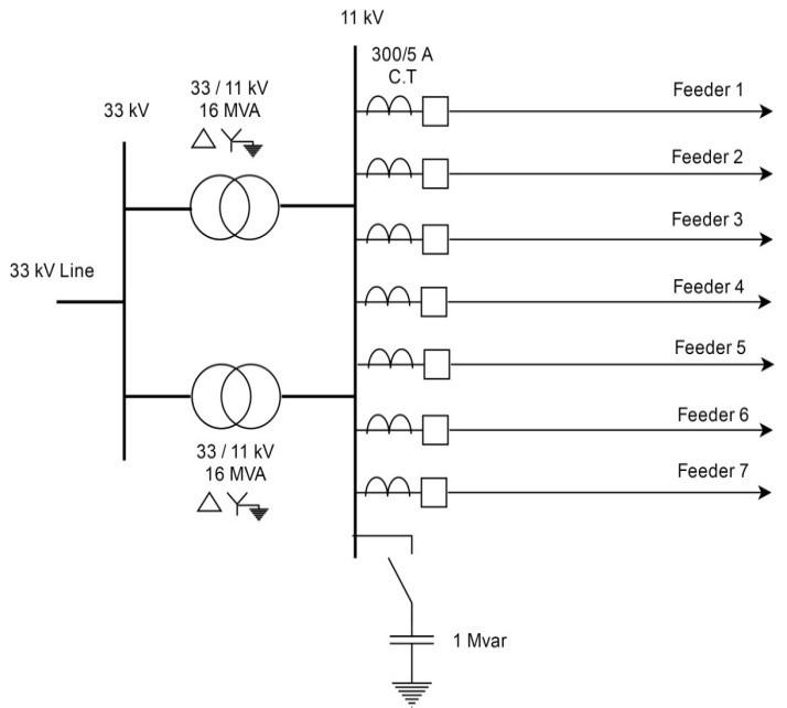
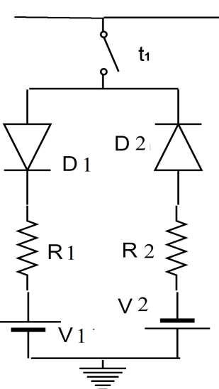
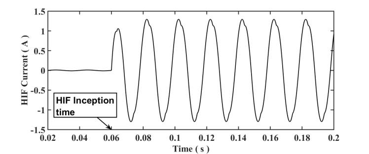
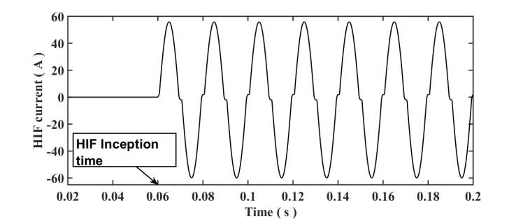
Figure3.HIFcurrentwaveform (a)R1=10000Ω,R2=9000Ω,V1=5000V,V2=5050V. (b)R1=150 Ω,R2=160 Ω, V1=2000V, V2=2050 V.
Lowpassfilters(LPF)and highpassfilters(HPF)isusedin DWTtodecomposea signalintoa lowfrequency and high-frequencycomponent. The decomposition process starts by passing a signalthrough LPF and HPF. The LPF produces an approximate coefficient which has high scaled and low-frequency decomposition. In contrast, the HPF produces detailed coefficient which has low scaled and high-frequency
High impedance
detection in distribution system (Kavaskar Sekar)
Int.J.ofAdv.inAppl. Sci. ISSN:2252-8814
97
fault
Figure 1.EPDNstudied
Figure 2.HIFmodel
(a)
(b)
decomposition. At once the first level of decomposition is completed, the sampling frequency is reduced by half of its value. To calculate the next DWT level, LPF output (approximation) is decomposed. The Daubechies basis db4, five level decomposition, and the sampling rate of 25.6 kHz with the data window length ofthreecyclesarechosenin thiswork.
Table1.Testconditions
Event Simulatedconditions
Total HIF Resistancesvariedfrom150Ω to12kΩandDCvoltagefrom1.5kVto10.5kV randomly
Loadswitching Changesinloadlevel:0%-25%,25%-50%,50%-75%,75%-100% and100%-110% bothforwardandreverseconditions.
NLLswitching Theratiooflineartonon-linearloadchanges1to0.5instepsof0.05bothinforwardand reverseconditions.
Capacitor
Switching Switchingconditionsonandoffwithloadvariationof25%,50%,75%,100%and125%.
Inrushcurrent Noloadswitchingof33/11kVtransformer
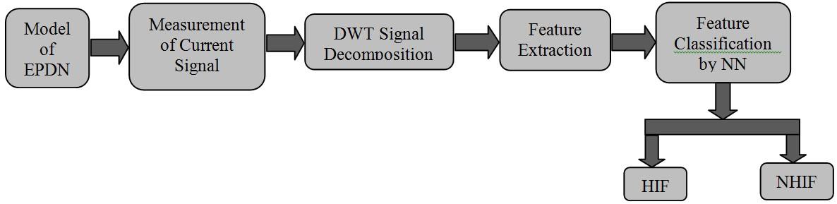
Figure 4.
540
90
216
90
64
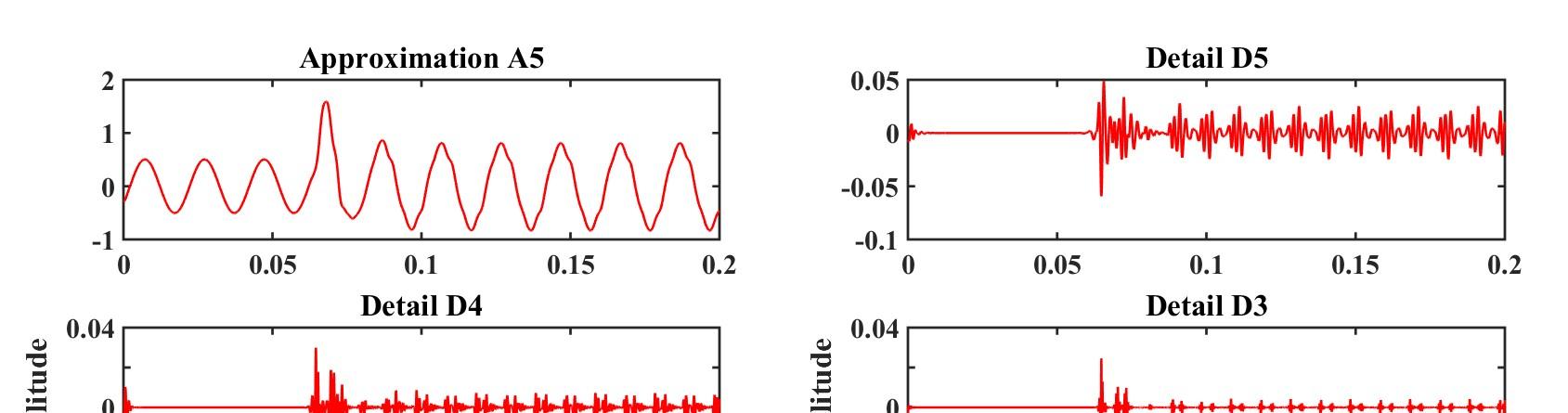
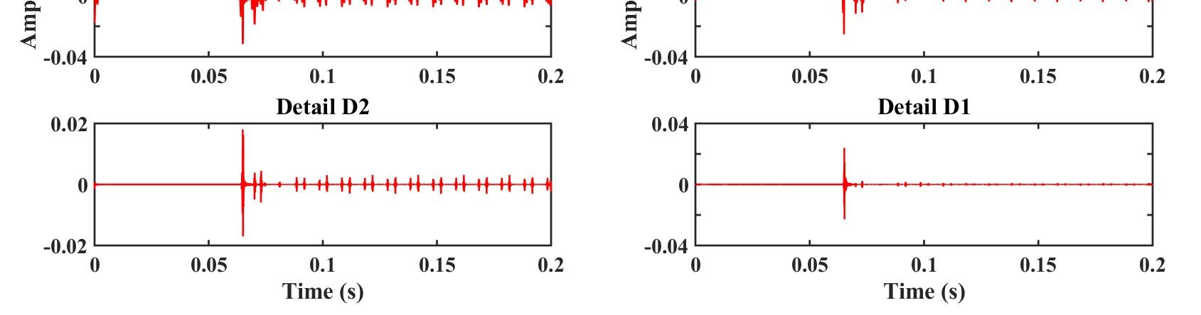
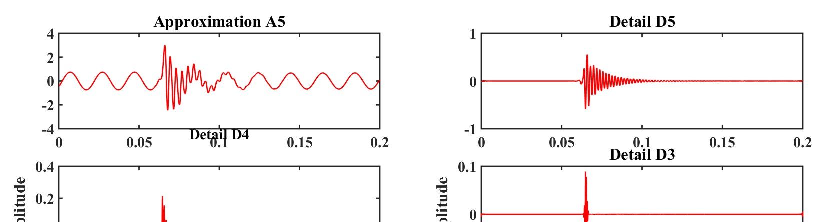
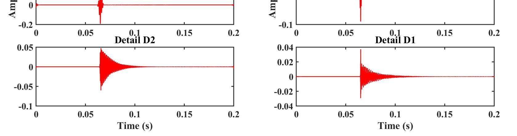
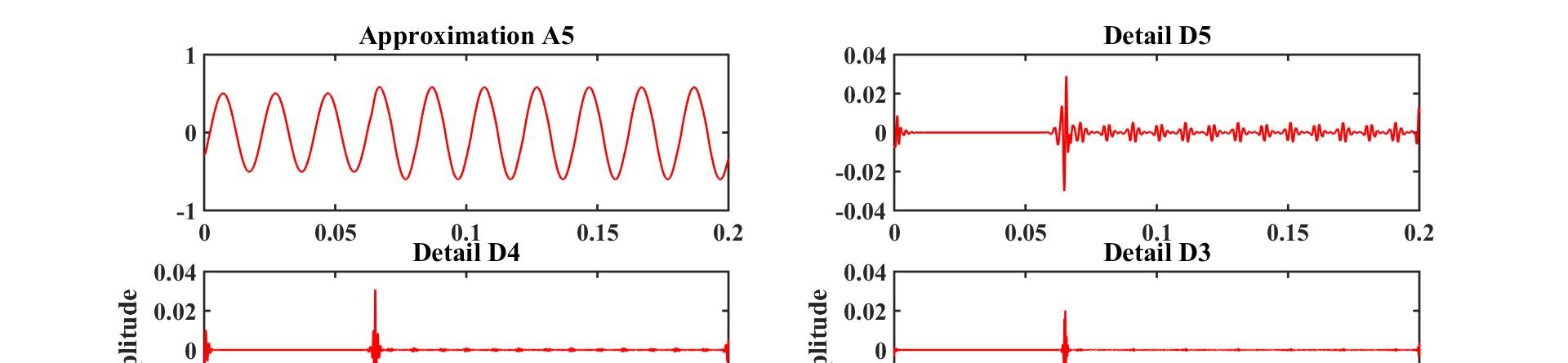
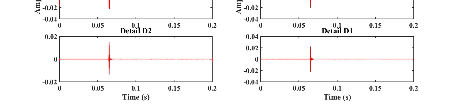
The decomposition of phase a current due to NLLs and capacitance switching at inception time of 0.065 s is shown in Figure 5 and Figure 6. It is found that the behavior of both NLL and capacitance haslow and high-frequency parts in all wavelet detail coefficient D5 to D1. The decomposition of phase a current during HIF is shown in Figure 7. A small magnitude of change in frequency component is present since the initiationofHIFindetailcoefficientD5alone.
3.2. Selectionofwaveletcoefficient
From the DWT analysis of the current signal, there were one approximation coefficient (A5) and five detailed coefficients (d1-d5) acquired. The comparison of different wavelet detail and approximation coefficient has been made to select wavelet coefficient for HIF Detection. It is observed that detail coefficients d4 and d5 offers diverse characteristics during different power system events and hence selected forfeatureextraction.
3.3. Featuresusingwaveletcoefficientsd4andd5
Six differentfeatureswereestimatedusingwaveletcoefficientsd4andd5aredescribedbelow:
a. Standard deviation:Itrepresentsthedeviationofasignalfromitsmean.
b. Energy:The totalenergycontentofthecurrentsignal.
Energy= ∫ i (t)dt (2)
c. Kurtosis:Biggerkurtosispointrepresentsmoreoutlierinthesignal.
Kurtosis= ( ) ( )( )( )∑( ) ( ) ( )( ) (3)
-Standarddeviation,�� –Mean,n –noofsampledata
d. Skewness:Itisameasureoftheirregularity oftheprobability distributionaboutitsmean.
ISSN:2252-8814 Int.J.ofAdv.inAppl. Sci.Vol. 8,No.2,June2019:95–102 98
The proposedHIFdetectionapproach
Skewness= ( )( )∑( ) (4)
High impedance fault detection in distribution system (Kavaskar Sekar)
Int.J.ofAdv.inAppl. Sci. ISSN:2252-8814
99
Figure5.DWTofcurrentsignalundernon-linearloadswitching
Figure 6.DWT of currentsignalundercapacitance switching
Figure 7.DWT of currentsignalunderHIF
e. Entropy:Itgivescomplexityofthesignal
Entropy=−∑p logp (5)
Where pjisanenergyprobabilitydistributionofWT detailcoefficient(d4and d5)
f. Sum:Sumofallpointsofsignal.
3.4. NNimplementation
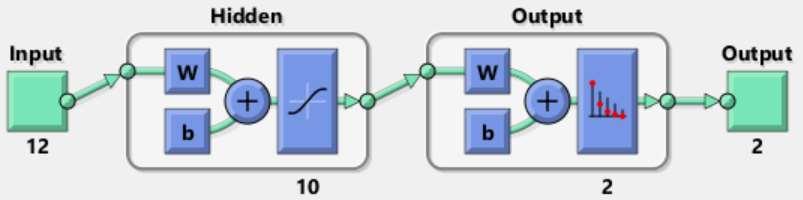
The NN is a powerful tool used in pattern recognition and classification [19]. Consequently, the proposed work uses NN to learn the input and outputrelationship from feature input vector. As mentioned in the feature extraction process, the input to NN comprises 12 elements (6 features of detail coefficients d4 and d5). The output layer has two neurons i.e. either HIF or NHIF and 10 hidden layers. A two-layer feedforward NN has been used in this work as shown in Figure 8. The sigmoid activation function used for hiddenlayer and softmax for the outputlayer.The NNistrained with scaled conjugate back-propagation that updatesweightandbiasvalues. Also, the number of epochswasdeterminedbyexperimentation.Thenumber of epochs for the training was set around 1000 and a mean squared error rate of e-03 was used [20]. The dataset is randomly divided into three parts: a training data set of 70%, validation of 15% dataset, and the remaining15%fortesting.
4.
RESULTSANDDISCUSSIONS
A set of 1000 features obtained by changing the simulation conditions as given in Table 1. Thus a widerange of studieshasbeen carried out to demonstrate the proposed method.Conversely, it is notpossible to report all information because of space constraint. The proposed method is evaluated through the following threeparameters:
- Dependability:Predicted HIFagainsttotalHIFconditions.
- Security:PredictedNon-HIFagainsttotalnon-HIFconditions.
- Accuracy:Actualpredictedagainstthe totalnumberofconditionsconsidered.
- Speed:Onecyclepowerfrequency current/Noofcyclesthatittakesto detectthe fault.
The confusion matrix of the NN during training, validation, and testing are presented in Figure 9. During training, all 370 HIF test cases are correctly classified to produce dependability of 100%. Two NHIF test case is misclassified as HIF to produce 99.4% security with the overall accuracy of 99.7%. During validation of 150 cases, dependability observed as 100%, and 97% of security with the overall accuracy of 98.7%. Finally, during testing of 150 cases, all HIF cases predicted correctly and only one NHIF cases are classified asHIFandproducedependability, security,and accuracyas100%,98.4%,and99.3%respectively. It is very clear from the confusion matrix that the method has an excellent detection rate. Nevertheless, there wasa huge amountofnon-linear loadvariation,alltheHIFcasesaredetected.
Power system more vulnerable to noise, it is necessary to investigate the proposed method with different Signal to Noise Ratio (SNR). Table 2 compares the performance under noisy atmosphere. It noted that the performance is similar to theone observed innormalcase for 10 dBof SNRon thesignal. For 20 dB of SNR, HIF detection rate alone same. However, the accuracy and security are reduced to 98% and 95.16% respectively. Additional SNR reduces all the three performance indices. Though the accuracy of 20 dB is less, theHIFdetectionrateisexcellent,andhencetheproposedmethod issuitableforSNRof20 orless.
ISSN:2252-8814 Int.J.ofAdv.inAppl. Sci.Vol. 8,No.2,June2019:95–102 100
Figure8.NNmodelforHIFdetection
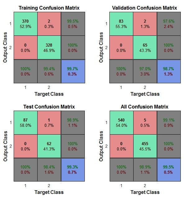
Table 3 shows the impact of the sampling rate of the proposed work. There was substantial upgrading demonstrated by the proposed methodology with sampling rate from 256 to 512. The detection rate diminishes as the sampling rate value decreases. Hence, the proposed scheme is better with 512 samplespercycle. Finally, the performance of the proposed HIF approach is compared with previously published articles as presented in Table 4. It is observed that all three performance indices are better than [4,7, 10, 14]. The speed of detection is compared with the references mentioned in Table 4. The speed of detection is low comparedto[4]and asgood aswith other referenceslisted in Table 4. However, it isnoted that HIFs arelow current, during which the distribution network are not in stress. As a result, the HIF detection speed is not a critical concern. In other hand, the security index of the HIF detection algorithm is important as well as its dependabilityindex.
Table 2.ImpactofSNRonthe proposedmethod
Table3.Impactofsamplingrateontheproposedmethod
Table 4.Comparisonoftheproposedmethodwithpreviouslypublishedwork
Int.J.ofAdv.inAppl. Sci. ISSN:2252-8814 High impedance fault detection in distribution system (Kavaskar Sekar) 101
Figure9.TheconfusionmatrixofNNs
Performanceindices 10dB 20dB 30dB Accuracy 99.33% 98.00% 93.33% Security 98.38% 95.16% 88.70% Dependability 100% 100% 96.59%
Performanceindices 512 420 256 Accuracy 99.33% 96.00% 86.66% Security 98.38% 95.16% 80.64% Dependability 100% 98.88% 90.90%
Method Accuracy(%) Security(%) Dependability(%) Speed Ref[4] 93.6 81.5 100 1 Ref[7] 97.3 96.3 98.3 0.04 Ref[14] 96 100 90 0.25 Ref[10] - 68 72 0.33 Theproposedmethod 99.33 98.38 100 0.33
5. CONCLUSION
In this paper, a new methodology based on the WT NNs is presented. The proposed method efficiently distinguishing HIF form other normal patterns. The proposed method comprehensively studied an actual electric power system with real data using MATLAB with a huge variation in power system operating conditions. The method has an exceptional detection rate even under wide variation in NLLs. This indicates that the proposed scheme is highly consistent and secure detection for HIFs with a dependability indexof100%.
REFERENCES
[1] Ghaderi, H., Mohammadpour, HA, Ginn, HL, and Shin, YJ, “HighImpedanceFaultdetection-a review,” Electr. Power Syst. Res,vol.146,pp.376-388,2017.
[2] Emanuel, D., Cyganski, J., Orr S., Shiller, and E. Gulachenski, “High impedance fault arcing on sandy soil in 15 kV distribution feeders: contributions to the evaluation of the low frequency spectrum,” IEEE Trans. Power Deliv, vol.5(2),pp.676-686,1990.
[3] Esmaeil, D. and Jamal, B., “High Impedance Fault Detection in Power Distribution Networks with Use of Current Harmonic-Based Algorithm,” Indonesian Journal of Electrical Engineering and Informatics, vol. 3(4), pp.216-223,2015.
[4] Ghaderi, H., Mohammadpour, HA, Ginn, HL, and Shin, YJ, “High impedance fault detection in distribution networkusing time-frequencybased algorithm,” IEEE Trans. Power Deliv,vol30(3),pp.1260-1268,2015.
[5] Samantaray, SR., Panigrahi, BK., and Dash, PK., “High-impedance fault detection in power distribution networks using time-frequency transform and probabilistic neural network,” IET Gener. Transm. Distrib, vol. 2(2), pp.261–270,2008.
[6] Soheili, A.,Sadeh, J.,and Bakhshi, R.,“ModifiedFFT-based high-impedancefaultdetection technique considering distribution non-linear loads: simulation and experimental study,” International Journal of Electrical Power and Energy Systems,vol.94,pp.124–140, 2018.
[7] Sarlak, M. and Shahrtash, SM., “High-impedancefaultdetection using combination ofmultilayerperceptron neural networks based on multi resolution morphological gradient features of current waveform,” IET Gener. Transm. Distrib,vol5(5),pp.588-595,2011.
[8] Kavaskar,S.andMohanty NK., “Combined mathematicalmorphologyand dataminingbasedhighimpedancefault detection,” Energy Procedia,vol.117,pp.417-423,2017.
[9] Hamid Mortazavi, S., Moravej, Z., and Mohammad, SS., “A hybrid method for arcing faults detection in large distributionnetworks,” International Journal of Electrical Power and Energy Systems,vol.94,pp.141–150,2018.
[10] Jichao, C., Toan, P., Trevor, B., Eliathambi, A., and Daming, Z., “Detection high impedance fault using current transformer forsensing and identification basedmethod on featuresextracted using wavelettransform,” IET Gener. Transm. Distrib,vol10(12),pp.2290-2298,2016.
[11] Santos, WC, Lopes, FV., Brito, NSD., and Souza, BA., “High-impedancefaultidentificationon distribution networks” IEEE Trans. Power Del,pp.32(1),pp.23-32,2017.
[12] Bakar, AHA., Ali, M., Tan, C., Mokhlis, H., Arof, H., and Illias, H., “High-impedance fault location in 11kV underground distribution systems using wavelet transforms” International Journal of Electrical Power and Energy Systems,vol.55,pp.723-730,2014.
[13] Mahari, H. and Seyed, “High impedance fault protection in transmission lines using a WPT-based algorithm,” International Journal of Electrical Power and Energy Systems,vol.67,pp.537-545,2015.
[14] Sedighi, AR., Haghifam, MR., and Malik, OP., “Softcomputingapplication inhigh impedance fault detection in distribution system,” Electr. Power Syst. Res,vol.76(1-3),pp.136-144,2005.
[15] Baqui, I, Zamora, I., Mazón, J., and Buigues, G., “High impedance fault detection methodology using wavelet transformandartificialneuralnetworks,” Electr. Power Syst, Res,vol.81(7),1325-1333,2011.
[16] Sergio, S., Pyramo, C., Maury, G., Alcyr, L., Franciele, A., and Daniel, L., “High impedance fault detection in power distribution systems using wavelet transform and evolving neural network,” Electric Power Systems Research,vol.154,pp.474-483.2018.
[17] Patrick, EF, Adriano, PM., Jean, PR., and Ghendy, C. “Non-linear high impedance fault distance estimation in power distribution systems: A continually online-trained neural network approach,” Electric Power Systems Research,vol.157,pp.20-28,2018.
[18] Kavaskar, S., Mohanty, NK, and Sahoo, AK. “High-impedancefault detection using wavelet transform,” IEEE conference on 2018 Technologies for Smart-City Energy Security and Power,pp.1-6, Bhubaneswar,2018.
[19] Bishop, CM, Neural Networks for Pattern Recognition.OxfordUniversityPress,1996.
[20] Adewole, AC.,Tzoneva, R., Shaheen, B., “Distribution network fault section identification and fault locationusing waveletentropy andneuralnetworks,” Applied Soft Computing,vol46,pp.296–306,2016.
ISSN:
Int.J.ofAdv.inAppl. Sci.Vol. 8,No.2,June2019:95–102 102
2252-8814
InternationalJournalofAdvancesinAppliedSciences(IJAAS) Vol.8,No.2, June2019,pp.103~116
ISSN:2252-8814,DOI:10.11591/ijaas.v8.i2.pp103-116
Frequencyregulationofmodernpowersystemusing novel hybridDE-DAalgorithm
SayantanSinha1,RanjanKumarMallick2
1DepartmentofElectricalEngineering,Siksha‘O’AnusandhanDeemedtobeUniversity,India
2DepartmentofElelctricalandElectronicsEngineering,Siksha‘O’AnusandhanDeemedtobeUniversity,India
ArticleInfo
Article history:
ReceivedAug30,2018
RevisedMar20,2019
Accepted Apr20,2019
Keywords: AGC
Benchmarkfunctions DEDAhybrid
Deregulated TID
ABSTRACT
An attempt has been made to regulate the frequency of an interconnected modernpowersystemusingautomaticgenerationcontrolunderarestructured market scenario. The system model considered consists of a thermal generation plant coupled with a gas turbine plant in both areas. The presence ofderegulatedmarketscenarioinaninterconnectedpowersystemmakesittoo vulnerabletosmallloaddisturbancegivingrisetofrequencyandtielinepower imbalances. An attempt has been made to introduce a novel Tilted Integral derivative controller to minimize the frequency and tie line power deviations andrestrictthemtoscheduledvalues.Amaidenattempthasbeenmadetotune thecontrollergainswiththehelpofanovelhybridoptimizationschemewhich includes the amalgamation of the exploitative nature of the Differential evolutiontechniqueandtheexplorativeattributesoftheDragonflyAlgorithm. Thishybrid technique is thereforecoined asDifferentialevolution-dragonfly algorithm(DE-DA)technique.Useofsomestandardbenchmarkfucntionsare made to prove the efficacy of the proposed scheme in tunig the controller gains. The supremacy of the proposed TID controller is examined under two individual market scenarios and under the effect of a step load disturbance. The robustness of the controller in minimizing frequency deviations in the systemsisbroadlyshowcased.Thesuperiorityofthecontrolleris alsoproved bycomparingitwithprepublishedresults.
Copyright © 2019 Institute of Advanced Engineering and Science. All rights reserved.
Corresponding Author:
SayantanSinha,
DepartmentofElectricalEngineering, Siksha‘O’Anusandhan Deemedto be University, KhandagiriMarg,2,SumHospitalRd,Bhubaneswar,Odisha751030,India. Email:sayantansinha51@gmail.com
1. INTRODUCTION
In recent days, the power system is in astate of transition from centralised control to restructured market scenario. The restructured market consists of GENCOs (Generation companies) DISCOs (Distribution companies), TRANSCOs (Transmission companies) and a control operator named as IndependentServiceOperator(ISO).Thecoordinatedcontrolofapowersystemofsuchahugescaleistedious andmuchmorecomplicated.TheprimefacieobjectiveofAGCinaninterconnecpedpowersystemistoensure that the deviations in frequency and the power flow in the tie-lines are restricted within nominal values. In a deregulated market scenario, the ISO plays an ancillary role in ensuring the stable operation of the power system [1, 2]. The main role of Automatic Generation control is to maintain an equity between the load demandsand the generation of each area.It also pays a keen attention to the fact that thefrequency deviation andthe tielinepowervariationsshouldstaywithinspecified limits[3].
Intherecentyearsmanyresearcheshavebeenmadebasedontheperformanceofautomaticgeneration control in the power system world like analysis of the power flow taking AGC into consideration in multi-area interconnected power grid taking into consideration the deregulated market scenario [4].
Journal homepage: http://iaescore.com/online/index.php/IJAAS
103
Paper [5] deals with the Utilisation of ultra-capacitor in load frequency control under restructured STPPthermal power systems using WOA optimised PIDN-FOPD controller. Paper [6] concentrates on automatic generation control of two-area hydro-thermal system considering governor dead band under deregulated environment. In paper [7], a work has been done on an algorithm technique known as symbiotic organisms searchforAGCintheinterlinkedpower environmentwhichincludeswindfarms.Arecentpaper[8]onAGC describes multiple unit of multiple area of deregulated power network by considering an algorithm method knownasnovel-quasioppositionalharmonysearch.Aresearchhasbeenmadeonthejudgmentoftheinfluence ofunreliabilityonAGCsystems[9].Amethod ofmodelingtechniqueand asurvey hasbeenmadeon system stability of AGC on radio systems in smart grids [10]. Paper [11] describes the safety games for threat minimizationinautomaticgenerationcontrol.Inpreviousyears,aworkhasbeendoneonamodelbasedstrike diagnosis and reduction for automatic generation control [12]. From the study of literature, it was found that the activity of the whole power system network depends on various optimization techniques, structure of the controller. So, the innovations of various optimization techniques are always a welcoming step for the role enhancement of automatic generation control of the entire power system. Many works have been done on various algorithm techniques and methods such as a flower pollination technique based AGC of interlinked power environment and cross characterized ‘gbest’-mentored gravitational search and marking search algorithm for AGC of multiple area power system [13,14].Several strategies have been made for control for automaticgenerationcontrolinmultiterminalDCgrids[15]andotherstrategiessuchasin[16],dividedmodel predictive control strategies with demand to power system automatic generation control and in paper [17], distributed automatic generation control using horizontal-based method for large perforation in generation of wind. In [18], an approach has been made to AGC with different nonlinearities by using two degrees of PID controller.Paper[19]bringstolighttheimplementationofanANFISbasedcontrollerfortheLoadfrequency studiesinderegulatedmarket.Loadandfrequencycontrolforaninterconnectedpowersystemusingfractional ordercontrollerswereeffectivelydiscussedin[20].
Inthisworkanattempthasbeenmade todevelopanovelcontrollerwiththe gainstunedbya hybrid optimization technique. The main objectives of the proposed work are: design of a novel tilted integral derivativecontrollerfor theAGCofamulti-sourcepowersystemunderderegulatedenvironmentasproposed in [21]; optimization of the gainsof the proposed controller with a hybrid DE-DA technique and comparison with the previously published results [21]; testing of the hybrid technique in some standard benchmark functions and establishing the superiority of the optimization scheme; analysis of the system dynamic parametersandcomparisonwiththeprepublishedresults[21] andtoestablishthe superiorityoftheproposed DE-DAoptimizedTIDcontroller overDEoptimizedPIDcontroller.
2. SYSTEMCONSIDERED
The system proposed in this work is a two area system having equal power ratings 2000 MW each. ThelinearizedtransferfunctionmodelofthesystemisclearlydepictedinFigure1.Eachareaisinclusiveofa thermalunitandagasgeneratingunit.Thethermalunitiscoupledwithareheatturbineinordertoincreaseits efficiency. The system parameters are listed down in Appendix A. Due to the presence of more than one GENCO in the system, the apf (ACE participation factor) is to be effectively chosen. APF stands for those coefficientsthatdistribute theACE(Areacontrolerror)amongtheGENCOs.
This paper incorporates the concept of a mutual contract that exists between the Distribution companies (DISCOs) and the generation companies (GENCOs) of an interconnected power system. This mutual contract can exist in various combinations and is well explained mathematically by the Distribution Participation Matrix (DPM). In a DPM, the GENCOsaredenoted by therowsand theDISCOsarelabeled in the columns. Every individual entry in the DPM gives us a picture of the fraction of the load that is in the contractbetweentheDISOCandthe correspondingGENCO.
Theactualtielinepowerflowcanbemathematicallyexpressedas
Thetielinepowerflowinaderegulatedenvironmentcanbeexplained as:
ISSN:2252-8814 Int.J.ofAdv.inAppl. Sci.Vol. 8,No.2,June2019:103–116 104
f2 f1 s T12 2 Ptieactual (1)
∆�� = ∑∑ ������ ∆�� − ∑∑ ������ ∆�� (2) ∆�� = �� − �� (3)
where
exp P and impP standsforthenetpowerexpectedtoflowfromarea1accordingtotheDISCOdemands and the power actually supplied to the DISCOs respectively. This gives rise to a deviation in tie line power whichismathematicallyexpressedas:
(4)
Theareacontrolerrorinderegulatedscheme canme expressedas:
(5)
Where the areacoefficientislabeled by 12α . 1β And 2β stands outas thefrequency biasconstants of the respective areas. In the proposed system there are morethan oneGENCOs and so the Area Control Error needsto be sharedbetweenallthe GENCOsproportionaltothe contributionsfor AGC.
3. CONTROLLERSTRUCTURE
The ProportionalIntegral Derivative (PID) controller is the most trusted feedback controller used so far. The PID controller accepts an error value as its input. The error is basically the difference between the system variable to be controller and a standard reference point. The control action is exercised using three gain parameters:
Proportionalterm[P]:mainlygovernedbyerroroccurring attimet
Integralterm[I]:governedbythesummationof allpasterror
Derivativeterm[D]:involvedin predictingerrorsoccurringatt+1.
Frequency regulation of modern power system using novel hybrid DE-DA algorithm (Sayantan Sinha)
ISSN:
Int.J.ofAdv.inAppl. Sci.
2252-8814
105
∆��
∆�� − ∆��
=
������ = ��∆�� + ∆��
������ = ��∆�� + �� ∆��
1sTt1 1 1sTg1 1 1sTr1 1sKr1Tr1 1sTp1 Kp1 1sTt2 1 1sTg2 1 1sTr2 1sKr2Tr2 1sTp1 Kp1 s 2*pi*T12 a12 R1 1 a12 B2 R2 1 Δf1 Δf2 cgsbg 1 1sYG 1sXG 1sTF 1sTcr 1sTcd 1 cgsbg 1 1sYG 1sXG 1sTF 1sT 1sTcd 1
(6)
Figure1.Linearisedtransferfunction modelofthesystem[18]
Thecontrolactionofa PIDcontrolcanbemathematically representedas:
Y(s)=�� +���� + (7)
Where Kp standsforthe proportionalgain, Ki standsfor theintegralgainand Kd denotes thedifferentialgain. This PID is a low order system buthasits applications inbroadareas. This typeof controller mainly finds its application in SISO( single input single output) system. MIMO (Multi input multi output) systems basically are divided into a number of SISO loops and a PID controller is employed for individual of them. The robustnessofthePIDcontrolleristhemainreasonforitswidespreadacceptanceinindustrialcontrol.However for an optimum operation of the PID controller, the selection of the above mentioned gains are of primeconcern.
3.1. Tiltedintegralderivativecontroller
The main objective of a Tilted Integral Derivative controller is to provide a feedback action as effective as the PID controller but with the results very close to the theoretical response. The TID controller has the proportional compensator of the PID controller replaced using a ‘tilt’ compensation. Mathematically the‘tilt’ canbe expressed by n s 1 .The tiltcompensatormainlygeneratesa frequencydependent feedbackgain with a tilt or a shape inclination towards the theoretical or conventional compensation value. As a result the compensation came to be termed as Tilted IntegralDerivative controller. The value of ‘n’ for the tiltfunction is between 2 and 3. When compared to the conventional PID controller, the coefficients of the respective transfer functions mainly has a value of 0,+1 or -1. On contrary the frequency coefficient in case of tilted controllerhasacoefficientof(1/n).Thiseffectivelyhelpstoimprovethecompensatingactionofthecontroller. TheschematicdiagramoftheTilted integralderivative controllerisgiveninFigure2.
4. OPTIMIZATIONTECHNIQUE
4.1. Differentialevolution
First coined by storn and price [22], the differential evolution is mainly known for its simplicity, efficacyand atremendoushighsenseofreliability.Itisby principle differentfromgeneticalgorithmbecause thetechnique of Genetic Algorithm stillrelies on crossover whereas Differential evolutionmainly focuses on mutationprocessforthegenerationofnewsolutions.
The successive difference between the two solutions of a randomly generated population mainly brings about the process of mutation. The optimization technique starts with the generation of a random populationofsizeN.Eachandeverymemberofthepopulationistobemaintainedwithinlimits.Theworkflow of the optimization technique mainly includes three processes namely mutation, crossover and selection. In this optimization scheme, two randomly generated populations are taken into considerationi.e the old population and the new population in which the members are generated from the old one by the process of mutationandcrossover.
The cross over operation done by mixing the mutant vector parameters with the target vector gives risetoatrialvector.Thetargetvectorinthenextgenerationissubstitutedbythetrialvector.Theevolutionary pathwayofDEisshownbelow:
ISSN:2252-8814 Int.J.ofAdv.inAppl. Sci.Vol. 8,No.2,June2019:103–116 106
n 1 s 1
Figure 2.The tiltedintegralderivative controller
PROPOSED
a. InitializationofarandompopulationofsizeNPconsistingofrealparametervectorsofsizeD.Iftheupper bound of the population is U j X and the lower bound is L J X then it is to be ensured that the randomly generatedpopulationsstaybetweenthelimits L J U J X X ,
b. Themutationprocessusuallydealswithavectorfromtheoldpopulationtoactasthetargetvectorforthe newgeneration.Themutationprocessismainlydonebycalculatedtheweighteddifferencebetweentwo randomly generated vectors and adding it to another randomly generated vector. The process can be mathematically expressed as:
WhereFCisa constantwhichvariesfrom(0,2).
c. Themainadvantageofhenewvectorgeneratedbymutationisthatitincreasesthediversityofthesearch space by a large extent. The crossover operation usually needs the addition of the mutant vector to the targetvector and formation ofa new vector. It basically involvesthree parents for the formation of their offspring’s.Mathematically itcanbeexpressed as:
In order to maintain the population size throughout the entire length of the process, the selection operationisnecessary.Thisoperationinvolvesthe targetvector Xi,G tobecomparedwithVi,G+1 and thebetter fitnesspossessing vectorattainsentrytothenewgeneration.
4.2. Dragonflyalgorithm
Brought to picture by Mirjalili [23], the dragonfly algorithm draws its inspiration from the steady streaming activities of the dragonflies. Supposedly small creatures and harming almost all other insects, the mostastonishingfactabouttheDragonfliesaretheirstrictlyadheredsocialbehaviour.Thereasonforswarming behaviourdisplayedbytheDragonfliesis forthepurpose ofhuntingand migration.Theprocessofhunting is discussed as feeding or static swarm and that of migration is termed as dynamic or migratoryswarm[24].
These two behavioural traits replicate the two main phases of optimization: exploration and exploitation.Thesetwophasescanbeexpressedasfollows:
Separation:thetermimpliesthetendencyofindividualstoavoidcollisionfromothernearbyindividuals in theirpathofmotion.
Alignment: The term stands for the matching of velocities of one individual with other in the entire population.
Cohesion:Thetermimpliesthetendencyofeachindividualtotraveltowardsthecentrepartofthegroup i.e.towardsthecentralsolution.
Attraction towards a food: This term mathematically implies the attractive behaviour of the dragonflies towardsanyrandomsourceoffood.
Distraction from enemy: the term correctly hints at the unique ability of the dragonflies to distract their enemytoaseparatecourse andsavingtheentirepopulation.
Takingintoconsiderationtheabovebehaviour oftheflies,theyaremathematicallymodelledas:
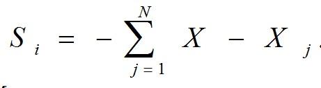
(10)
Where Si is the separation vector and X is the position of the current individual and Xj is the position of thejth individual. (11)
Int.J.ofAdv.inAppl. Sci. ISSN:2252-8814 Frequency regulation of modern power system using novel hybrid DE-DA
107
algorithm (Sayantan Sinha)
����,��+1= ����1,��+����(����1,��− ����2,��) (8)
,,1, ,,1 ,,1, .....(9) jiGjirand jiG jiGjirand VifrandCRorjI U XifrandCRorjI (9)
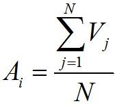
Where Ai isthealignmentvectorand Vj isthe velocity ofthe currentindividualthatistobematchedwiththe restoftheswarm. (12)
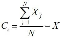
Where Ci is the cohesion vector, N indicates the number of particles, Xj indicates the position of the current particleand Xindicatesthecentralsolutionasdiscussedabove.
(13)
Where X+ andXdenotesthecurrentindividualposition andthatofthesourceoffood respectively.
(14)
Where X- andX standsforthepositionofthecurrentdragonflyand itsenemyrespectively. Thestepvectorfortheupdationofthedragonflypositioncanbecalculatedasthesummationofallthesefactors andcanbe mathematically expressedas:
(15)
Afterthegenerationofthestepvector,thepositionofthedragonfliesisupdatedas:
(16)
In the absence of any neighboring immediate solution., the dragonflies position is put to updation using a randomwalkpatternnamelycalledtheLevyflight.Thusthepositioncanbemathematicallyexpressedas:
(17)
Where dstandsforthe distancethatistobe coveredby Levyflightphenomena.
5. HYBRID OPTIMIZATIONSCHEME
A novel attempt has been made to bring about the amalgamation of the exploitative abilities of an evolutionary computation scheme namely the Differential Evolution and the explorative abilities of a swarm intelligence namely a Dragonfly Algorithm. The technique so developed was coined as Differential Evolution-DragonflyAlgorithm(DE-DA).TheentirecodehasbeendevelopedinMATLAb2013bplatform.
Use of some standard unimodal and multimodal benchmark fucntions has been used for testing the efficacy anfthesupremacyofthedesinednovelhybrid DE–DA technique.
In order to prevent any slight bit of anomaly in the comparisons, the function evaluation parameters are considered thesame for all the considered fucntions. The hybrid codesare simulated for 30 timesand the results were put to statistical analysis. Table 2 summarizes these results. For each method the worst, mean, median,best, andstandarddeviationfromthe30 independentrunswerecalculatedandcompared.
In order to establish the robustness of the proposed hybrid technique, the standard deviation and the mean of the fitness values obtained over 30 iterations are calculated and observed. Lesser value of standard deviationindicatestheequitythatexistsinthesolutionsover30runs.Thisinfersthatanalgorithmwithlesser valueofstandarddeviationismore likelytobeconsistent.
ISSN:2252-8814 Int.J.ofAdv.inAppl. Sci.Vol. 8,No.2,June2019:103–116 108
X
X Fi
X
X Ei
Xi w eEi fFi cCi aAi sSi 1 Xt
1 Xt Xt 1 Xt
t t t X d Levy X X ) ( 1
6. ANALYSISFOR DE-DA
The best values, worst values, mean values and standard deviation values for the above mentioned eightbenchmarkfunctionsinTable1.Table2clearlyindicatesthatthevaluesofthestatisticalparametersare theleast for theDE-DA hybrid technique. The resultswereobtainedfor100 iterations. Added tothistheDEDA also accounts for the lowest value of standard deviations among the three techniques. This low value of standarddeviationimpliesthatthesolutionsobtainedforthe30 iterationsareapproximatelyconstantandthis isatestforconsistency oftheproposedoptimization scheme.Figure 3,Figure4,Figure5,Figure 6,Figure7, Figure8,Figure9, andFigure10areshowingtheconvergencecurveofDE,DAandDE-DAin 8functions.
Int.J.ofAdv.inAppl. Sci. ISSN:2252-8814
109 Function name Testfunction N S fo pt Sphere n 1 i 2 i 1 x (x) F 30 n100,100] [ 0 Schwefel n 1 i i n 1 i i 2 x x (x) F 30 n10,10] [ 0 Rotated hyper ellipsoid n 1 i i 1 j 2 j 3 ) x ( (x) F 30 n100,100] [ 0 Schwefel x} i ,1 x max (x) F i 4 30 n100,100] [ 0 Step n 1 i 2 i 5 5]) 0 ([x (x) F 30 n100,100] [ 0 Ackley e 20 ) n 1 i xi cos2 n exp(1 n 1 i xi2) n 1 2 0 20exp( F6(x) 30 n32,32] [ 0 Griewank function n 1 i xi xisin( F7 30 n500,500] [ 0 Penalised n 1 i n 1 i u(xi,10,100,4) 1)] yi 10sin2(3 1)2[1 (yi yi) 10sin2( n F8(x) 4 1 x 1 y i i 30 n50,50] [ 0 Functionname METHOD BEST WORST MEAN STD F1 DE 12.5817 72.6387 35.2792 16.5974 DA 18.1680 58.8918 35.3926 10.0163 DE-DA 7.5605 55.6477 30.0650 12.9463 F2 DE 1.95e+04 1.07e+07 1.92e+06 2.311e+06 DA 1.26e+04 8.001e+07 4.96e+06 1.445e+07 DE-DA 228.6165 1.57e+07 9062e+05 2.9932e+06 F3 DE 1.16e+3 1.26e+04 6.194e+03 5.76e+03 DA 1.12e+03 1.22e+04 4.27e+03 4.56e+03 DE-DA 47.8718 2.19e+03 748.8607 871.0934 F4 DE 0.2221 3.0569 0.8643 0.6937 DA 0.0553 10.1392 2.2868 2.3062 DE-DA 0.0248 1.4754 0.3595 0.3832 F5 DE 45.4651 150.5548 102.1089 25.2523 DA 40.8339 107.4640 71.5784 21.2027 DE-DA 6.0574 41.2643 17.1603 9.9018 MULTIMODAL
F6 DE 14.1712 20.2920 18.6768 1.6130 DA 6.2233 19.9485 15.6799 3.1122 DE-DA 3.2943 16.1654 9.4173 3.3874 F7 DE 6.4211 124.8288 49.3711 39.0981 DA 3.4524 75.4961 30.1153 20.4420 DE-DA 0.6638 36.7725 6.7834 9.1282 F8 DE 14.0331 7.454e+7 7.9e+6 1.66e+5 DA 3.2985 1.3e+7 1.3e+6 2.7e+6 DE-DA 0.1777 2e+6 1.65e+5 4.3e+5
Frequency regulation of modern power system using novel hybrid DE-DA algorithm (Sayantan Sinha)
FUNCTIONS
Figure3.Convergence curveofDE, DAand DE-DAforfunction1
Figure 4.ConvergencecurveofDE,DAand DE-DAforfunction2
Figure 5.ConvergencecurveofDE,DAand DE-DAforfunction3
Figure6.ConvergencecurveofDE,DAand DE-DAforfunction4
Figure7.ConvergencecurveofDE,DAand DE-DAforfunction5
Figure8.ConvergencecurveofDE,DAand DE-DAforfunction6
ISSN:2252-8814 Int.J.
Adv.inAppl. Sci.
8,
June
103–116 110
of
Vol.
No.2,
2019:
7. APPLICATION OFDE-DA TOAGCPROBLEM
The proposed hybrid Differential evolution - Dragonfly Algorithm is effectively implemented for obtainingtheoptimalgainparametersoftheTiltedIntegralDerivativecontroller.Thehybridalgorithmissaid to have a better performance than the De and DA as shown in Table 2. Table 3 lists down the optimal values of the controller gains. The application of the hybrid algorithm to the AGC is governed by the following pseudocode.
Pseudocode forthehybridoptimization:
Generation of the initial population and specification of the Differential evolution parameters like cross overratioandmutation frequency.
Computationofthefitnessfunctionsofeachofthepopulationmembers.
Generationofoffspringsusingmutationtechnique.
Calculationof the fitnessfunctionofeach generatedoffspring.
Selectionofthebestoffspringbycrossovertechnique thatincludestheparent.
Replacementoftheparentsinthetotalpopulationwiththeoffspringsandgiverisetoafinalpopulation. ThefinalDEpopulationactsasthe initialpopulationforDragonflyAlgorithm.
Initializationof thestepvectors Xi
Computationofthefitnessvaluesofallthedragonflies.
Updationofthefood sourceandtheenemyposition.
Updation of cohesion vector, separation vector, alignment vector, food distance vector and the enemy attack vector.
Based on condition of at least one dragonfly in the neighbourhood of the current dragonfly, updation of thepositionisdone.
Checkingofthenewparticlesunderboundaryconditions.
Jump overtostep2untilmaximumiterationisreached.
Terminate theloop.
8. RESULTSANDANALYSIS
ThediscussedtwoareapowersystemmodelisputtosimulationwiththehelpofMATLAB/Simulink.
Thetiltedintegralderivativecontrollerisemployedinthiscaseasthesecondarycontrollerforminimizingthe AreaControlError (ACE) tozero. Thegainsofthe TIDcontroller areset to optimalvalues with thehelp of a novelhybridDE-DAtechnique.Theobjectivefunctionsemployedin thetuningprocessareasfollows:
Int.J.ofAdv.inAppl. Sci. ISSN:2252-8814 Frequency
of modern power
111
regulation
system using novel hybrid DE-DA algorithm (Sayantan Sinha)
Figure9.Convergence curveofDE, DAand DE-DAforfunction7
Figure 10.Convergencecurveof DE,DAand DE-DAforfunction8
t 0 dt ptie f2 f1 IAE (15) t 0 tdt ptie f2 ff ITAE (16) t 0 dt 2 ptie 2f2 2f1 ISE (17)
Thevaluesofeachoftheaboveobjectivefunctionsduringthetuningprocessisnotedandscriptedin Table2.ThetableclearlyindicatesthatthevalueoftheobjectivefunctionJistheminimuminthecaseofISE (Integralsquareerror)and henceforthallthetuningprocessinthe paperhasbeendone consideringISEasthe costfunction.
Table 1.Optimizedsystemparametersby hybridDE-DAtechnique
Table 2.Objectivefunctionvaluesforbase caseandbilateraltransactions
Theanalysisisdoneontwocases: Case 1:the base case
In thiscase theGENCOs and DISCOs come into mutualparticipation for theelectricity market over acommonarea.ThisimpliesDISCOsofoneareacanonlycomeincontractwiththeGENCOsoftherespective areas. This mutual contract scenario can be represented with the help of Distribution Participation Matrix (DPM).
(19)
The area participation factor apf is taken equal for all the GENCOs in this particular case. Soapf1 =apf2 = apf3 =apf4 =0.5
The simulation is carried out inclusive of a SLP of 0.01 pu in area 1. The demands of DISCOs are generally fixed at 0.1 MW. Figure 11, Figure 12 and Figure 13 represents the frequency deviation in area 1 ( f1 ),area2frequencydeviation( f2 )andtielinepowerflowdeviation( ptie )respectively.Table3clearly gives us the values of settling time, maximum overshoot and minimum undershoot for the DE DA optimized TIDcontroller.Effectivecomparisonhasbeendonewiththesettlingtime,maximumovershootandminimum undershoot of DE optimized PID controller when applied tothe same physical system under base case. From thetabularcomparisonitcanbeeasilyinferredthattheDE-DA tunedTIDcontrollerismuchmorerobustand effective thantheDetunedPIDcontroller.Figure14,Figure 15,Figure16and Figure17elaboratesthepower outputpatternofGENCO1,GENCO2, GENCO 3andGENCO4respectively.
Figure11 Frequencydeviation ofarea1
Figure12 Frequencydeviation ofarea 2
ISSN:2252-8814 Int.J.ofAdv.inAppl. Sci.Vol. 8,No.2,June2019:103–116 112 t 0 tdt 2 ptie 2f2 2f1 ITSE (18)
Marketscenario Kt1 Kd1 Ki1 Kt2 Kd2 Ki2 Basecase 0.2401 0.2802 0.1590 0.1539 0.0952 0.1302 Billateralcontract 0.2556 0.1503 0.3057 0.1995 0.1976 0.2974
Marketscenario Objectivefunction ITAE IAE ITSE ISE Basecase 1.9137 0.5937 0.0782 0.0398 Billateraltransaction 1.6242 0.5898 0.0837 0.0409
0 0 0 0 0 0 0 0 0 0 05 05 0 0 0.5 0.5 DPM
13.Tielinepowerdeviation
14.PowersuppliedbyGENCO1
15.PowersuppliedbyGENCO2
Figure 16 PowersuppliedbyGENCO3
17.PowersuppliedbyGENCO 4
Case 2:Billateraltransaction
In this case the DISOCs and the GENCOs of both area come to a mutual contract participation and thescenarioisexpressedbythefollowingDPM.
Theareaparticipationfactorinthiscase istakenasreferenceto[18]. apf1=0.75;apf2=1-apf1=0.25;apf3=apf4 =0.5.Thegiven systemis simulated underbilateralcontractscenario subjecttoasteploadperturbationof0.01pu.Figure18,Figure19andFigure20clearlyportraysthefrequency deviation in area 1 ( f1 ), area 2 frequency deviation ( f2 ) and tie line power flow deviation ( ptie ) respectively.Table4listsdownthevaluesofthe settlingtime, maximumovershootandminimumundershoot
Frequency regulation of modern power system using novel hybrid DE-DA algorithm (Sayantan Sinha)
Int.J.ofAdv.inAppl. Sci. ISSN:2252-8814
113
Figure
Figure
Figure
Figure
0 0 025 03 07 1 025 0 0 0 025 02 03 0 025 05 DPM (20)
for the hybrid optimized TID controller and is put to comparison with DE optimized PID controller [18].
Figure 21, Figure 22, Figure 23 and Figure 24 clearly portrays the power output of GENCO 1, GENCO 2, GENCO3andGENCO4 respectively.ThecomparisonclearlyindicatesthesuperiorityofDE-DAoptimized TIDcontrolleroverDEoptimizedPID controllerunderbilateralcontractscenario.
2252-8814 Int.J.ofAdv.inAppl. Sci.Vol. 8,No.2,June2019:103–116
ISSN:
114
Figure18 Frequencyoscillationsinarea1
Figure19 Frequencyoscillationsinarea2
Figure20 Tie linepowervariations
Figure 21 PowersuppliedbyGENCO1
Figure22 PowersuppliedbyGENCO2
Figure23 PowersuppliedbyGENCO3
Figure24.PowersuppliedbyGENCO 4
Table3.Dynamic systemparametersunderbasecasescenario
Table4.Dynamic systemparametersforbilateralscenario
9. CONCLUSION
Whenever a modern interconnected power system is considered for study under restructured market scenarios, the power system becomes highly sensible to slight load disturbances. As of concern the maintainenceoffrequencywithinscheduledvaluesshouldbeofamajorimportance.Thisiseffectivelyattained by the Tilted Integral Derivative controller in the proposed work. Development of a hybrid optimization technique, the DE-DA technique is successfully verified and tested with standard benchmark functions. This technique is thereafter used to provide optimal values to the controller for minimizing the ACE to zero. The hybridtunedcontrollerhasprovedtobeeffectiveinminimizingfrequencyaswellastielinepowerdeviations in a shortesttime period possible. In order to justify the supremacy ofthecontroller, the results are compared withprepublishedresults.Thedynamicperformanceindicesofthesystemisanalysedinboththecasesandis listeddowninrespectivetablesforclearinference.Itcanbeclearlyestablishedthatthevaluesofsettlingtime, maximum overshoot and minimum undershoot is considerably less for both market scenarios taken intoconsideration.
REFERENCES
[1] Dong, X., Sun, H., Wang, C., Yun, Z., Wang, Y., Zhao, P., Ding, Y., and Wang, Y., “Power Flow Analysis ConsideringAutomatic Generation Control forMulti-Area Interconnection PowerNetworks,” IEEE Transactions on Industry Applications,vol53(6),pp.5200-8,2017.
[2] Kumar, J., Ng, KH., and Sheble, G., “AGC simulator for price-based operation. I. A model,” IEEE Transactions on Power Systems,vol.12(2),pp.527-32,1997.
[3] Kumar, J., Ng, KH., and Sheble, G., “AGC simulator for price-based operation. II. Case study results,” IEEE Transactions on Power Systems,vol.12(2),pp.533-8,1997.
[4] Sinha, N., Lai, LL., and Rao, VG., “GA optimized PID controllers for automatic generation control of two area reheat thermal systems under deregulated environment,” Electric Utility Deregulation and Restructuring and Power Technologies, 2008. DRPT 2008,pp.1186-1191,2008.
[5] Saha,A.andSaikia,LC.,“Utilisationofultra-capacitorinloadfrequencycontrolunderrestructuredSTPP-thermal power systems using WOA optimised PIDN-FOPD controller,” IET Generation, Transmission & Distribution, vol.11(13),pp.3318-31,2017.
[6] Raju,M.,Saikia,LC.,Sinha,N.,andSaha,D,“Applicationofantlionoptimizertechniqueinrestructuredautomatic generation control of two-area hydro-thermal system considering governor dead band," Power and Advanced Computing Technologies (i-PACT),pp.1-6,2017.
[7] Hasanien, HM. and El-Fergany, AA, “Symbiotic organisms search algorithm for automatic generation control of interconnected power systems including wind farms,” IET Generation, Transmission & Distribution, vol. 11(7), pp.1692-700,2016.
[8] Shiva, CK. and Mukherjee, V., “Automatic generation controlofmulti-unit multi-area deregulated power system using a novel quasi-oppositional harmony search algorithm,” IET Generation, Transmission & Distribution, vol.9(15),pp.2398-408,2015.
Frequency regulation of modern power system using novel hybrid DE-DA algorithm (Sayantan Sinha)
Int.J.ofAdv.inAppl. Sci. ISSN:2252-8814
115
Controllertype Systemdata Settlingtime Maximumovershoot Minimumundershoot PID[18] f1 5.52 0.0409 -0.2574 f2 4.51 0.012 -0.0946 ptie 1.88 0.0057 -0.0315 TID f1 4.4831 0.3500 -0.0090 f2 4.420 0.9400 -0.0055 ptie 7.0473 0.0057 -0.0315
Controllertype Systemdata Settlingtime Maximumovershoot Minimumundershoot PID[18] f1 10.87 0.0988 -0.4664 f2 11.47 0.0683 -0.2158 ptie 3.08 0.05 -0.0185 TID f1 7.6598 0.1149 -0.1551 f2 7.1017 0.1096 -0.0975 ptie 9.4850 0.0083 -0.0348
[9] Apostolopoulou, D., Domínguez-García, AD., and Sauer PW., “An assessment of the impact of uncertainty on automaticgenerationcontrolsystems,” IEEE Transactions on Power Systems,vol.31(4),pp.2657-65,2016.
[10] Liu,S.,Liu,PX.,andElSaddik,A.,“Modelingandstabilityanalysisofautomaticgenerationcontrolovercognitive radio networks in smart grids,” IEEE Transactions on Systems, Man, and Cybernetics: Systems, vol. 45(2), pp.223-34,2015
[11] Law, YW, Alpcan, T., and Palaniswami, M., “Security games for risk minimization in automatic generation control,” IEEE Transactions on Power Systems,vol.30(1),pp.223-32,2015.
[12] Sridhar,S. andGovindarasu,M.,“Model-based attack detectionand mitigation forautomaticgeneration control,” IEEE Transactions on Smart Grid,vol.5(2),pp.580-91,2014.
[13] Jagatheesan, K., Anand,B., Samanta, S., Dey,N., Santhi, V., Ashour, AS.,and Balas VE, “Applicationofflower pollination algorithm in load frequency control of multi-area interconnected power system with nonlinearity,” Neural Computing and Applications,vol28(1),475-88,2017.
[14] Khadanga,RK.andKumar,A.,“Hybridadaptive‘gbest’-guidedgravitationalsearchandpattern searchalgorithm for automatic generation control of multi-area power system,” IET Generation, Transmission & Distribution, vol.11(13),pp.3257-67,2016.
[15] McNamara, P., Meere, R., O'Donnell, T., and McLoone, S., “Control strategies for automatic generation control overMTDCgrids,” Control Engineering Practice,vol.54,pp.129-39,2016.
[16] Venkat, AN.,Hiskens,IA., Rawlings, JB.and Wright, SJ.,“Distributed MPC strategieswith applicationto power system automatic generation control,” IEEE transactions on control systems technology, vol. 16(6), pp.1192-206,2008.
[17] Variani,MH.andTomsovic,K.,“Distributedautomaticgenerationcontrolusingflatness-basedapproachforhigh penetration ofwindgeneration,” IEEE Transactions on Power Systems,vol.28(3),pp.3002-9,2013.
[18] Ibrahim, AN., Shafei, MA., and Ibrahim, DK., “Linearized biogeography based optimization tuned PID-P controller for load frequency control of interconnected power system,” Power Systems Conference (MEPCON), pp.1081-1087,2017.
[19] Selvaraju, RK. and Somaskandan, G., “ACS algorithm tuned ANFIS-based controller for LFC in deregulated environment,” Journal of Applied Research and Technology,vol.15(2),pp.152-66,2017.
[20] Gorripotu, TS., Sahu, RK., and Panda, S., “AGC of a multi-area power system under deregulated environment using redox flow batteries and interline power flow controller,” Engineering Science and Technology, an International Journal,vol.18(4),pp.555-78,2015.
[21] Hota, PK. and Mohanty B., ”Automatic generation control of multi source power generation under deregulated environment,” International Journal of Electrical Power and Energy Systems,vol.75,pp.205-14,2016.
[22] Storn, R. and Price, K., “Differential evolution–a simple and efficient heuristic for global optimization over continuousspaces,” Journal of global optimization,vol.11(4),pp.341-59,1997
[23] Mirjalili, S., “Dragonfly algorithm: a new meta-heuristic optimization technique for solving single-objective, discrete,andmulti-objectiveproblems,” Neural Computing and Applications,vol.27(4),pp.1053-73,2016.
[24] KS SR, Murugan, S., “Memory based hybrid dragonfly algorithm for numerical optimization problems,” Expert Systems with Applications,vol.83,pp.63-78,2017.
ISSN:
Int.J.ofAdv.inAppl. Sci.Vol. 8,No.2,June2019:103–116 116
2252-8814
InternationalJournalofAdvancesinAppliedSciences(IJAAS) Vol.8,No.2, June2019,pp.117~124
ISSN:2252-8814,DOI:10.11591/ijaas.v8.i2.pp117-124
EnhancedperformanceofPIDloadfrequencycontroller forpowersystems
DolaGobindaPadhan,SureshKumar Tummala EEEDepartment,GokarajuRangaraju InstituteofEngineering andTechnology,India
Article Info
Article history:
ReceivedSep8, 2018
RevisedMar 27,2019
AcceptedApr29,2019
Keywords:
Complementarysensitivity
Kharitonov’stheorem
Loadfrequency control(LFC)
PID
Corresponding Author:
ABSTRACT
A novel control structure for designing a PID load frequency controller for power systems is presented. The controller with a single tuning parameter is designed based on a desired closed-loop complementary sensitivity function and Pade approximation. Comparative analysis demonstrates that proposed PID controllers improves the settling time and reduces overshoot effectively againstsmall steploaddisturbances.Also,theperformanceandrobustness of the controllers have been analyzed and compared. Simulation results show significantly improvedperformanceswhencomparedwithrecentresults.
Copyright © 2019 Institute of Advanced Engineering and Science. All rights reserved.
DolaGobindaPadhan, EEEDepartment, Gokaraju RangarajuInstituteof EngineeringandTechnology, SurveyNo.288 NizampetRoad,KrishnajaHills,Bachupally, Kukatpally, Hyderabad,Telangana500090,India.
Email:dg.padhan@griet.ac.in
1. INTRODUCTION
Frequency deviation in Power System due to variation between generation and load shall be rectified within a fraction of seconds resulting in stability and security. Load Frequency Control (LFC) of an extensive power framework can be alluded as the issue of controlling the recurrence by directing the created units with reaction to change in stack [1]. For framework soundness, LFC must furnish recurrence with zero enduring state mistakes and tie-line trade varieties, high damping of recurrence motions and diminishing overshoot of the unsettling influence. The objectives specified are conveyed effectively in past works by variouscreatorsutilizing Fuzzy rationale PI and PIDcontrollers[2, 3], idealcontrol[4,5].Variable structure control[6,7],versatileand self-tuning control[8,9].Downtheline,different tuning ruleshave pickedupthe consideration for the previously mentioned goals in which Internal Model Control (IMC) [10] is one among them. The LFC PID controller configuration utilizing Laurent arrangement is clarified by Padhan and Majhi [11]. Double PI controller tuning utilizing swam enhancement calculation is introduced in [12]. The two-degree-of-freedom internal modelcontrol schemesuggested by Tan [10] consists of two controllers with two tuning parameters where simultaneous tuning of the two parameters is difficult. In practice, a simple control structure with a fewer number of tuning parameters is desirable. The proposed control structure (see Figure 1) for LFC design consists of only one controller (Gc). Kasireddy et.al designed a PID controller for LFCthroughreducedmodelorder[13].
Journal homepage: http://iaescore.com/online/index.php/IJAAS
117

In Figure 1, G and Gme−θm represent the power system dynamics and its model, respectively. For LFC, controller design is inconvenient because G results in higher order plant models, which are approximated bylowerordertransferfunctionswithtimedelayusinga relay-basedidentification method. This paper has been alienated into 6 sections. Modeling of power system dynamics with necessary derivations discourse in section 2. In section 3, the PID controller design method is discussed followed by Section 4 in which the simulation results are presented. Section 5 deals with Robustness analysis and performanceofa powersystemusingKharitonov’srectanglesfollowedby conclusionsinsection6.
2. MODELINGOFPOWERSYSTEMDYNAMICS
Figure 2 shows single area power systems with a linear model. From Figure 2 it can be noticed that the power is supplied to the single area by a single generator. There are two types of turbine used for a generation:(a)non-reheated (NRT)andreheated(RT).
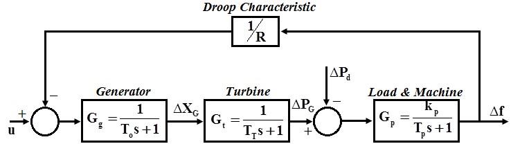
TheplantmodelusedforLFCwithoutdroopcharacteristicsis gtp G = GGG (1)
Where Gg, Gt, and Gp are the dynamics of the governor, turbine, and load & machine, respectively. For a reheatedturbine,
Where Tr is a constant and c is the portion of the power generated by the reheat turbine in the total generated power.Fornon-reheatedturbineTr =0.Theplantmodelused forLFCwithdroopcharacteristicis
gtp gtp GGG
G = 1GGG/R (2)
From(1)and(2)can berepresentedbythe second-ordertransferfunctionmodel
ISSN:2252-8814
Adv.inAppl.
117–124 118
Int.J.of
Sci.Vol. 8,No.2,June2019:
Figure1.Proposedcontrolstructure
Figure2.Singleareapowersystem
r t rT cTs1 G= Ts1Ts1
Statespaceequationsinthe Jordancanonicalformbecome m x(t)Ax(t)bu(t) (4)
y(t)cx(t) (5)
When a relay test is performed with symmetrical relay of height ±h, then the expression for the limit cycle output for 0 ≤
is
Let the half period of the limit cycle output be τ. Then the expression for the limit cycle output for θm ≤ t
τ is
Theconditionforalimitcycleoutputcanbe written as y(0)cx(0)y()0
Substitutionof t = τ in (7) anduse of (6) givestheinitialvalueofthecyclingstates
When tp is the time instant at which the positive peak output occurs and tp ≥ θm, then the expression of the peakoutput Ap becomes
andthe expressionforthepeaktimebecomes
SubstitutionofA,
Int.J.ofAdv.inAppl. Sci. ISSN:2252-8814
119 ms 12 Gke = Ts1Ts1 (3)
Enhanced performance of PID load frequency controller for power systems (Dola Gobinda Padhan)
Where 1 12 2 1 0 T1kA; b = ; c =1111TT 0 T
≤ θ
At1At
t
m
y(t)cex(0)cAeIbh (6)
(7)
≤
mm A(t)A(t) 1 m y(t)cex()cAeIbh
(8)
m 1 A() A1A x(0)IeA2eeIbh
(9)
pmpm A(t)A(t) 1 pm Acex()AeIbh (10)
1 2 /T 12 pm /T 12 TT 1e tln TT 1e (11)
2m111m22 /T()/T/T/T()/T/T 12 T1e2ee1T1e2ee10 (12) 12 121212 TT /T/TTTTT p Akh21e1e1 (13)
b,andc in(9)and(10)give
The (11-13) are solved simultaneously to estimate θm, T1 and T2 from the measurements of , Ap and tp The relentlessstategain k is thoughttobe knownfrom the earlierorcanbe assessedfrom astage flag test. Care hasbeen taken to explain the arrangementofnon-directconditions, so intermingling may notoccur toa falsearrangement.
3. PIDCONTROLLERDESIGN
Thenominalcomplementarysensitivity functionforloaddisturbancerejection canbe obtainedas
GG
= 1GG (14)
To rejecta stepchangeintheloadofthepowersystem, theasymptoticconstraintshouldbesatisfied sothattheclosed loopinternalstability canbeachieved[3].
(15)
Thedesired closed-loopcomplementarysensitivityfunctionisproposedas
(16)
Where βisthe only tuning parameter for obtainingthe desired performance of thepowersystem. As there always exists a trade-off between the nominal performance and robust performance, β must be tuned accordingtothedesiredchoice.α1 andα2 canbeobtained from(15)and theconstraintas
Using(14),(15)andsecondorder Pade´approximationforthetime delay term,weget
The(18)canbe writtenintheformofaPID controllerwithlead/lagfilteras
ISSN:
Int.J.ofAdv.inAppl. Sci.Vol. 8,No.2,June2019:117–124 120
2252-8814
c
c
T
12 11 s,TT lim1T0
m 2 21 s 4 ss1 Te s1
m1m2 44 22/T/T 12 12 1 21 T1e1T1e1 TT TT and m2 4 /T 2 2221 2 T1e1T T (17)
22 2121 c 2 21 o oo 6ss1lsls1 G mm kmsss1 mm (18) Where 21m 1 6T6T4 l 6 2 121m2mm 2 6TT4T4T l 6 0m1m6246 22 1m2m1m m366162 223 2m2mm m242424
4. SIMULATIONRESULTS
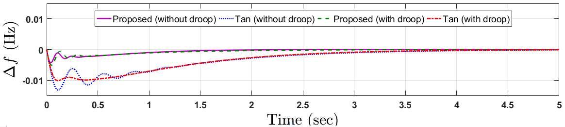
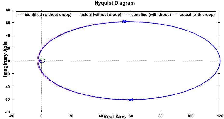
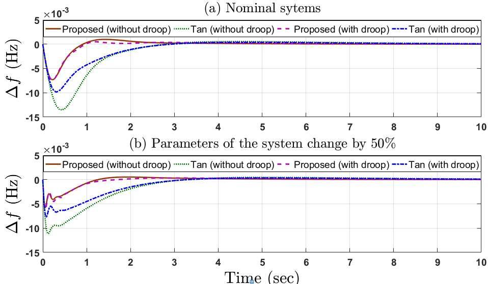
Consider a power system with a non-reheated and a reheated turbine whose model parameters are given by KP = 120, TP = 20, TT = 0.3, TG = 0.08, R = 2.4, Tr = 4.2 and c = 0.35 [11]. The identified models and controller settings (see Table 1) for the power system with non-reheated and reheated turbines are obtained using (11-13, 17). The Nyquist plots of the identified and actual models are shown in Figure 4 to illustrate the accuracy of the identification method. To get stable and robust response, β values in Table 1 are obtained from extensive simulation studies. Figure 3 and Figure 5 show the frequency change of the power system following a load demand ΔPd = 0.01. The stability robustness is tested by changing the parameters of the system by 50%. From the simulation results, it is evident that the proposed method gives significantly improvedperformancesthantheTan’smethod.
Table1. Controlparametersforidentifiedmodel
IdentifiedModel ControlParameters
NRT(WD)
NRT(D)
RT(WD)
0.05s 2 250e 2.028s12.765s106.2
0.541s 120e 23.2137s10.9057s1
RT(D) 0.035s 2 235.3e 1.79s16.9s100
Kc=2.0245,Ti=0.5005,Td=0.1332,a1=29.0238, a2=15.1661,b1=28.6982,b2=5.77239,β=0.01
Kc=0.7192,Ti=0.2075,Td=0.1159,a1=0.9212, a2=0.1411,b1=0.1515,b2=0.0234,β=0.07
Kc=3.6549,Ti=0.5797,Td=0.2355,a1=24.4801, a2=29.7725,b1=24.0884,b2=20.2681,β=0.01
Kc=1.0619,Ti=0.2107,Td=0.1828,a1=1.154, a2=0.1323,b1=0.1973,b2=0.0231,β=0.065
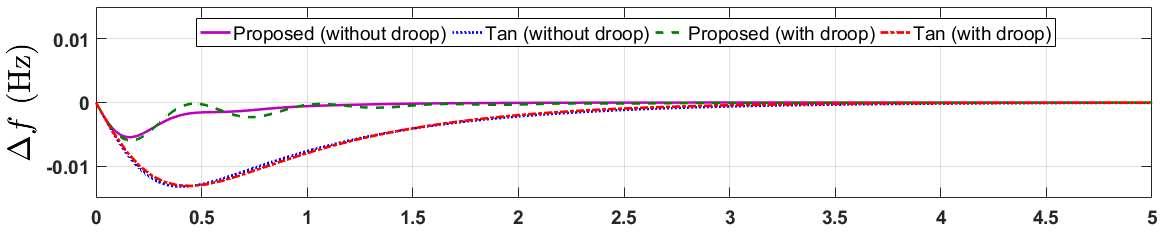
(a)Nominalsystems
(b)Parametersofthesystemchangeby50%
Figure 3.Frequencydeviationof the closedloopsystemwithnon-reheatedturbine
Int.J.ofAdv.inAppl. Sci. ISSN:2252-8814 Enhanced performance of PID load frequency controller for power systems
121 2 21 ccd 2 2 21 asas1 1 GK1Ts Ts bsbs1 (19) Where 1 c 0 K6 km i1T 2 d 1 T 22al 11al 2 2 0 bm m 1 1 0 bm m
(Dola Gobinda Padhan)
ModelType
0.4626s 120e 28.4952s10.2202s1
5. ROBUSTNESSANALYSISANDPERFORMANCE
In this section, Robustness of the system has been analyzed using Kharitonov’s Theorem. Closedloop characteristic equation CL(s) and denominator of the closed-loop transfer function T(s) are the polynomials that make the control system stable. Considering the forward-path and feedback-path transfer functionsG(s)andH(s),characteristic equationis
CL(s) = 1+G(s)H(s) = 0
CLnn110 (s)asas......asa
(20)
For simplicity, assume that theleading coefficient an isconstantand the coefficientshavebeen normalizedso that an = 1. Thepolynomialcoefficientscanthenbeexpressedas
so,thecharacteristicequationbecomes
(s)sas......asa
ISSN:2252-8814 Int.
ofAdv.inAppl. Sci.
8,
June2019:117–124 122
J.
Vol.
No.2,
Figure4.Nyquistplotsforthepowersystemwith non-reheatedturbine
Figure5.Frequencydeviationoftheclosedloopsystemwithreheated turbine
nn1
minmax iii aa,a, i=0,1.......n-1 (21)
nn1 CLn110
(22)
Int.J.ofAdv.inAppl.Sci. ISSN:2252-8814
AccordingtoKharitonov’sTheorem,annth-degreeintervalpolynomialfamilydescribedby (1a)and(1b)isrobustlystableifandonlyifeachofthefourKharitonovpolynomialsisstable,thatis,allthe rootsofthosepolynomialshavestrictlynegativerealparts
Forthesystem
Thecharacteristicequationis
For±10%variationsinthecoefficientsofthepolynomial,Theintervalsofthepolynomialwillbecome
Figure6showsKharitonov’srectanglesrotatearoundtheorigininacounter-clockwisedirectionto satisfythemonotonicphaseincreasepropertyofHurwitzpolynomials.Forclarity,thegraphiszoomedin Figure7toshowthezero-exclusionpoint.AstheKharitonov’srectanglesdonotpassthroughtheorigin,itis concludedthattheclosedloopsystemguaranteestherobuststability.
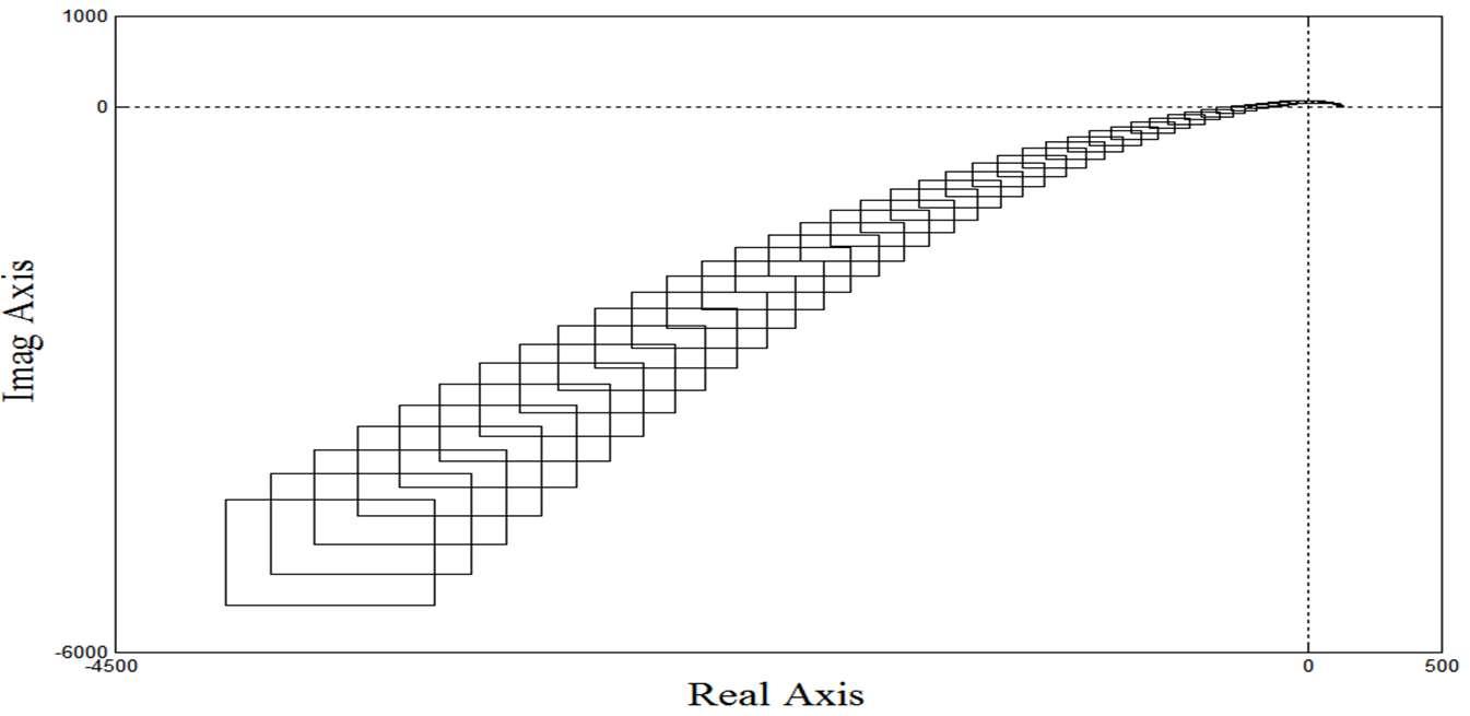
Figure6.Responseofthesystemwith±10%variationsinthecoefficientsof polynomialonthecomplexplane
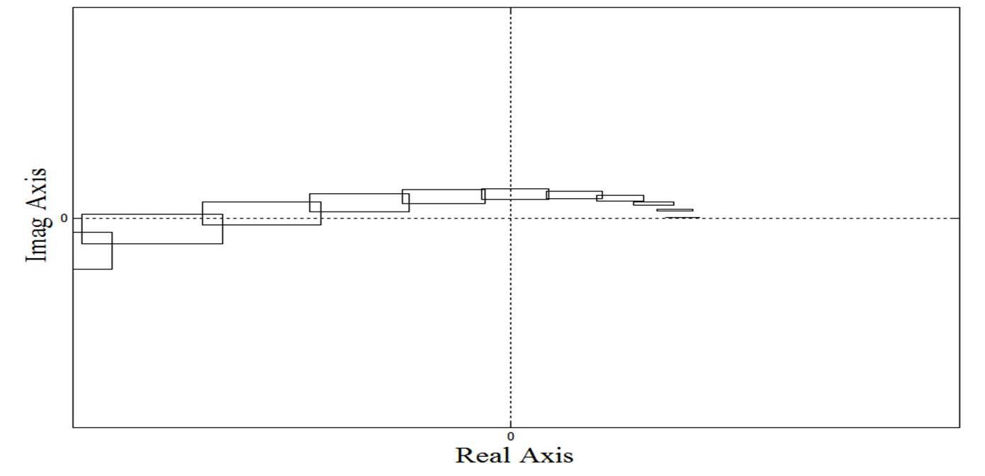
Figure7.Responseofthesystemshowingzeroexclusionpoint
EnhancedperformanceofPIDloadfrequencycontrollerforpowersystems(DolaGobindaPadhan)
123
120G(s)0.08s10.3s120s1
32 CL(s)0.48s7.624s20.38s1210 (23)
3210 a0.528,0.432a8.3864,6.8616a22.418,18.342a133.1,108.9
Table 2 shows it is observed that the proposed method gives less Integral Absolute Error (IAE), Integral Squared Error (ISE) and Integral Time Absolute Error (ITAE) as compared to Tan’s method, so closed loop performance is improved. If we compare the total variations of the control signals, the results of both methods are almost same. Thus, with same control signals, the proposed method gives comparatively fewererrors.
Table2.Variouserrorsand totalvariations TypeofModel
6. CONCLUSION
The Load Frequency Characteristics of a single-area power system with non-reheated and reheated turbines have been deliberated. The proposed method is flexible and gives satisfactory performance in nominal as well as the perturbed case. The proposed PID controller with a new control structure and a single tuning parameter (β) gave better performance than Tan’s controller. By showing the zero exclusion point by Kharitonov’s rectangles, it guarantees the robust stability for closed loop power systems. The proposed schemecaneasilybeextendedto multi-areapowersystems
REFERENCES
[1] R. K. Cavin, M. C. Budge, and P. Rasmussen, “An optimal linear system approach to load frequency control,” IEEE Trans. Power App. Systems, vol. 90(6),pp.2472-2482,1971.
[2] C. E. Fosha and O. I. Elgerd, “The megawatt-frequency control problem: A new approach via optimal control theory,” IEEE Trans. Power App. Systems,vol.89(4),pp.563-567,1972.
[3] N. N. Bengiamin and W. C. Chan, “Variable structure control of electric power generation,” IEEE Trans. Power App. Systems,vol.101(2),pp.376-380,1982.
[4] M. A. Sheirah and M. M. Abd-EI-Fattah, “Improved load frequency self-tuning regulator.,” Int. J. Control, vol.39(1),pp.143-158,1984.
[5] P.Kundur, Power System Stability and Control.McGrawHill,NewYork1994.
[6] C. T. Pan and C. M. Liaw, “An adaptive controller for power system load-frequency control,” IEEE Trans. Power Systems,vol.4(1),pp.122-128,1989.
[7] J. Talaq and F. Al-Basri, “Adaptive fuzzy gain scheduling for load frequency control,” IEEE Trans. Power Systems,vol.14(1),pp.145-150,1999.
[8] M. F. Hossain, T. Takahashi, M. G. Rabbani, M. R. I. Sheikh, and M. Anower, “Fuzzy-proportional integral controller for an AGC in a single area power system,” Proc. 4th Int. Conf. Electrical and Computer Engineering, Dhaka,Bangladesh,pp.120-123,2006.
[9] S. Majhi, “Relay based identification of processes with time delay,” Journal of process control, vol. 17, pp.93-101,2007.
[10] W. Tan, “Unified tuning of PID load frequency controller for power systems via IMC,” IEEE Transactions on Power Systems,vol.25(1),pp.341-350,2010.
[11] D. G. Padhan and S. Majhi, “ANew Control SchemeforPIDLoadFrequency Controllerof Single-area and MultiareaPowerSystems,” ISA Transactions,vol.52,pp.242–251,2013.
[12] M. Elsisi, M. Soliman, M. A. S. Aboelela, and W. Mansour, “Dual Proportional integral controller of Two-Area Load Frequency control based gravitational search algorithm,” Telkomnika Indonesian Journal of Electrical Engineering and Computer Science,vol.15(3),pp.397-406.2015.
[13] Idamakanti Kasireddy, Abdul Wahid Nasir, and Arun Kumar Singh., “Non-integer IMC based PID design for load frequency control of power system through reduced model order,” International Journal of Electrical and Computer Engineering,vol.8(2),pp.837-844,2018.
ISSN:2252-8814 Int.J.ofAdv.inAppl. Sci.Vol. 8,No.2,June2019:117–124 124
IntegralTime AbsoluteError IntegralAbsolute Error IntegralSquared Error Totalvariations NRT(WD)-Tan 0.5164 0.1061 0.001494 0.0199 NRT(WD)-Proposed 0.5147 0.1008 0.001184 0.0127 NRT(D)-Tan 0.5303 0.106 0.001363 0.0214 NRT(D)-Proposed 0.521 0.1007 0.001175 0.0189 RT(WD)-Tan 2.002 0.2007 0.002254 0.0735 RT(WD)-Proposed 2.058 0.2061 0.002273 0.07906 RT(D)-Tan 2.006 0.2007 0.01223 0.0729 RT(D)-Proposed 1.966 0.2006 0.002264 0.0797
InternationalJournalofAdvancesinAppliedSciences(IJAAS) Vol.8,No.2, June2019,pp.125~135
ISSN:2252-8814,DOI:10.11591/ijaas.v8.i2.pp125-135
Solarirradianceforecastingusingfuzzylogicandmultilinear regressionapproach:AcasestudyofPunjab,India
SahilMehta,PrasenjitBasak
ElectricalandInstrumentationEngineeringDepartment,ThaparInstituteofEngineeringandTechnology,India
ArticleInfo
Article history:
ReceivedSep11,2018
RevisedApr5,2019
Accepted May2,2019
Keywords:
Forecasting Fuzzylogic
Microgridplanning
Multilinearregression
Solarirradiance
ABSTRACT
The accurate forecasting of solar irradiance depends on various uncertain parameters like time of day, temperature, wind speed, humidity, and atmosphericpressure.AlltheseplayanimportantroleincalculatingPVpower output.Inthispaper,anovelapproachforforecastingofsolarirradianceusing flexible and accurate fuzzy logic and robust multi-linear regression approach has been proposed considering the above mentioned five variables. Based on the simultaneous consideration of those five variables, the solar irradiance is forecasted using the proposed methodology at a particular location in India, and the results are compared with the real time measured value of solar irradianceatthatlocationonthedaysforwhichsolarirradianceareforecasted. Theproposedmethodisvalidatedbycomparingtheresultswithrealtimedata. The error analysis of the fuzzy logic based proposed system shows the root mean square error of 10.011 and mean absolute percentage error of 1.703%, while compared with real time data measured by instruments pyranometer, anemometer etc. The same results are found better while compared with the resultsobtainedusingmultilinearregression approach
Copyright © 2019 Institute of Advanced Engineering and Science. All rights reserved.
Corresponding Author:
PrasenjitBasak,
ElectricalandInstrumentationEngineeringDepartment, ThaparInstitute ofengineeringandTechnology, 147004Patiala,Punjab,India.
Email:prasenjit@thapar.edu
1. INTRODUCTION
In the present energy scenario, the depletion of the natural fossil fuels, increased environmental pollutionandtheeffectofageingoftheinstalledpowerplantsarebecomingachallengeforthe society.Thus, integratingtherenewableenergysources(REs)withthegridisoneofthekeysolutionstosuchproblems.But thisintegration also leads to some major challengesand problems likethe uncertain nature of these resources especiallysolarintermsofpowergenerationisacriticalissue.Thesesustainableformsofenergydependsand vary according to the weather conditions like temperature, atmospheric pressure, humidity, wind speed and also the time of the day. Apart from these parameters, the solar power generation mainly depends upon the solar irradiancewhich furtherdependsupon thevariousweather basedparameters.Thus,theforemoststep in solarpowerpredictionsystemsistheforecastingofGlobalHorizontalIrradiance(GHI)[1].
Focusingon thebenefitsofRESforecasting,in arecenttime,anumberofstudieson solarirradiance forecastinghavebeenproposed,mostofwhichrequirethehistoricaldataofthe dependentparameters.In[2], number of existing techniques for forecasting, their advantages and computation requirements has been discussed.Also,thevariouschallengesfacedbyincreasedpenetrationofrenewableenergyresourcesinpower systemaswellasmicrogridhavebeenbrieflydiscussed.In[3],astudybasedondemandresponseofanisolated microgridundertheimpactofuncertaintiesinrenewableenergyforecastsanditsperformancehasbeenstudied. The result shows less influence of uncertainty in solar than that in wind power on the dispatch cost at the generating end and for the management of the flexible loads. The energy management system for an isolated
Journal homepage: http://iaescore.com/online/index.php/IJAAS
125
microgrid with PV,ESS and electric vehicles using thehybrid solar irradianceforecasting methodology for a shortperiodof timehasbeenpresented in [4]. The proposed methodology, basedon thedata available online from satellite and the data of clear sky for the selected microgrid location uses Heliosat algorithm for determiningthe cloudcoverfromthe satellitedata.In [5],the problemofshorttermforecastingtheestimated PVpowerforplanningofamicrogridhasbeensolvedusingneuralnetworks.Thehistoricaldataofparameters likePVproduction,globalirradianceforlearningandtrainingavailableatthetestfacilityhasbeenconsidered. In [6], using the Markov switching model, solar forecasting for a remote microgrid has been presented. The proposed method uses the previous data available on the online portals for solar irradiance and clear sky irradiance,whereasusingFourierexpansion,linearmodelfordifferentconditionshavebeencreatedforsunny, mildlycloudyandextremelycloudydays.Overcomingtheproblemofuncertaintyinmicrogridintegratedwith renewable sources of energy,holt-winters forecasting method has been used in [7]. The proposed forecasting methodology has been incorporated in the microgrid simulation with assumed residential load and battery storage system as back up source. The results of the work give an idea of reduced cost by forecasting the accurate value of solar in terms of energy management system (EMS) for a microgrid. The performance of intelligentneuralnetwork(NN)toolandstatisticallinearregressiontoolforforecastingthePVoutputhasbeen analyzedin[8].Using thepreviousonlineavailable dataforsolarirradiance,temperature,training andtesting of the multilayer feed forward neural network have been done. The results show artificial NN (ANN) tool to be more accurate and flexible whereas statistical regression being more robust and easy to construct. In [9], short term solar irradiance forecasting focusing on the variable nature of the weather conditions as well as dependent radiation. The work compares seasonal autoregressive (SAR) linear models for solar irradiance forecastingwiththenonlinearmodels,i.e.nonlinearautoregressive(NAR)basedoncomputationalintelligence technique and regression tree (RT). In [10], long term load demand forecasting using a regression based approach has been presented. The work focuses on various variables like historical data of the local power utilitycompany,thepresentnumberofconsumersanddevelopmentplansofthesetlocation.
Shorttermloadforecastingforbigdata,i.e.hugehistoricaldataforvariousinputparametersaffecting the forecasting has been considered in [11]. Being more deterministic and robust multi linear regression methodology hasbeenused for accurate forecasting.Varioussensorsand data science applications, historical dataforloadforecastinghasbeenused.Focusingonthehighmatrixformulations,leastnumberofparameters are considered with big data. The results of the work show 3.99% of the MAPE, considered to be under the tolerable limits. In [12], the forecasting of the electricity consumption in Thailand, as a case study, has been presented using artificial neural network and multi linear regression. Using the ANN technique theminimum cost of generation is calculated. Using the multi linear regression algorithm, depending on historical data of various parameters, electricity consumption has been calculated. In [13], dependent upon various meteorologicalparametersliketemperature,dewpoint,humidity,visibility,windspeedandweathersummary, shorttermsolarirradianceforecastinghasbeenproposed.Usingtheavailablemeteorologicaldatafromvarious onlinesources,theforecastingproblemhasformulatedasastructuredoutputpredictionproblem.Theproposed algorithm of long-short term memory has been compared with least square regression, persistence algorithm anddifferentNNtechniques.Basedonhistoricaldataforcloudcoveri.e.inputparameterslikeazimuth,zenith angle and time of day. In [14], forecasting of solar irradiance using Labview software and regression based numerical algorithm has been proposed. Initially, dependent upon the parameters, solar irradiance has been forecasted and further combined with the local available temperature PV power output has been forecasted. [15] Presents multi-linear regression based solar power probabilistic forecasting, working with various inputs available at the weather stations. The system performance depends upon the cloud movement or the clear sky index is rated as better performance under the clear sky conditions. The results show that the accuracy of the system increases with the increase in historical data. In [16], the combined effect of relative humidity (RH) and air temperature (AT) on solar irradiance forecasting have been explored. Using the multivariate linear regression analysis carried out in different temperature range, the results come out to be moreaccurate andreliableincomparison tosinglevariabledependentforecasting.Also,forecastingusingthe flexiblefuzzylogicapproachhasbeenintrendamongvariousauthorsintherecentyears.In[17],focusingon thefutureaspectsofenergyplanning,varioustechniqueslikeneuralnetworks,geneticalgorithmandspecially fuzzylogicapproachalongwiththeitsapplicationandadvantagesovertheother;intermsofforecastinghave been discussed. Overcoming the problem of uncertainty in weather conditions, in [18] solar radiation forecastingusingfuzzyandneuralnetapproachhasbeendone.Theresultsshowthehigheraccuracyleveland thusitsapplicationinthegridconnectedPVsystem.Similarto[18],consideringthemeteorologicalparameters likeskyinformation,clearnessindexandtemperature;solarradiationforecastingusingafunctionalfuzzylogic approach has been suggested in [19]. Forecasting of solar energy using the fuzzy logic approach have been donefocusingontheneedofavailablesolarenergydatain[20]consideringthesunshineperhour,temperature, latitude and longitude and time of year. With the increasing need of accurate forecasting using a fuzzy logic approach, forecasting of solar irradiance has been suggested in [21] normalizing the inputs and output to
ISSN:
Int.J.ofAdv.inAppl. Sci.Vol. 8,No.2,June2019: 125–135 126
2252-8814
eliminate convergence problems. The results show a high accuracy level of forecasted value with respect to measuredvalueforshorttermforecasting.
Inarecenttrend,i.e.planninganddesigningofamicrogridwithinstalledRES,in[22]thefuzzylogic approachforforecastingofrenewableenergybasedsourcesconsideringthedataofmeteorologicalparameters ofa setlocationhasbeenshown.Thecomparativeresultsshowbetteraccuracyofthefuzzylogicapproach in comparison to the neural network and vector autoregressive forecasting models. With the increasing need of forecasting in microgrid applications, in [23] the focus is on energy management system, i.e. uncertain renewableenergybasedsourceandvariableload.Forthispurpose,arealmicrogridsysteminChilewithwind and PV and variable load have beenconsidered and day ahead forecastingusing the fuzzylogicapproachhas beencarriedout.Hence,fortheplanningofamicrogridconsideringparticularlongitudeandlatitude,itisvery necessary to have the accurate forecasted value of energy generation through the available renewable energyresources.
Thus,fromtheliteraturesurveyusingthehistoricaldataavailableattheonlineportals,theindividual effect offewmeteorologicalparameterssuchas temperature, sky movement,cloudcover,humidity andwind onsolarirradianceforecastinghasbeenstudied.Itisobservedthatthecombinedeffectoffiveparameterssuch as temperature, wind, humidity, time of day and the atmospheric pressure at the location has not been consideredsimultaneouslyforsolarirradianceforecastingbecauseofcomplexsystemcharacteristics.
Onthebasisofabovediscussionthemainobjectiveofthepresentworkhavebeenconsideredassolar irradiance forecasting and power calculation using the high dimension fuzzy logic and multilinear regression approach.Inhighdimensionfuzzylogicapproachalargenumberofrules(1200)combiningtheeffectofabove mentioned parameters are formed to get more reliable and accurate results whereas, the robust multilinear regression (MLR) approach has also been implemented to develop the mathematical relation between all the parameters and forecasted solar irradiance for different time intervals. For the purpose of validation, the forecastedvaluesofsolarirradiance,astheoutputofbothfuzzylogicandmultilinearregressionapproach,are compared with the real time solar irradiance using Pyranometer device. The work presented in this paper is organized as follows: The introduction of the article is covered in section 1 followed by description of measuring devices and data collection methodology in section 2. The design and development of the high dimensional fuzzy logic system and multilinear regression approach have been discussed in section 3. The results and discussion for the proposed approach is presented in section 4 and the conclusions in section 5 followedbyreferences.
2. MEASURINGDEVICESANDDATA COLLECTION
Focusing on the major objective of work, the data collection of various parameters is initiated. The parametersareidentifiedastemperaturein°C,windspeedinm/s,humidityinpercentage,timeofdayinhours: minutes,atmosphericpressureinhectopascals(hpa)andsolarirradianceinW/m2.Theadvantageofmeasuring and collecting the actual real time data at a specific location is the high accuracy and system reliability. In Section2.1(A),2.1(B)and2.1(C)thedevicesusedforthemeasurementofsuchparametersatthesetlocation at30.356008, 76.372142(30°21′21.63″N and76°22′19.71″E)in theThaparUniversitycampushavebeen discussedalong with thedata loggingsystemin2.1(D).
2.1. Measuring
devices
2.1.1.Pyranometer
The Pyranometer device; Hand-Held terminal model (HHT-13) used for the measurement of global horizontalirradianceisshowninFigure1(a).ItisaportableelectronicdevicetowhichtheGHIsensorshown inFigure1(b)canbeattached.ThemajorbenefitofusingtheHHT-13terminalmodelformeasuringtheGHI is the data logging facility. The real time GHI for a specific location can be stored as well as logged in the personallaptopsusingtheinstalledsoftware.
2.1.2.Anemometer
The multipurpose device used to measure various meteorological parameters is the Lutron AM4214SD Hotwire Anemometer shown in Figure1 (c).Thisdevice isused to measure variousparameterslike wind speed in m/s as well as in km/hr, temperature in °C and °F; and humidity in percentage in the real time. The benefit of such a device is the online monitoring as well as the data logging option which offers flexible operationofthedevice.The figure showstheanemometerdeviceconnectedtooneofthe twoseparateprobes which are usedfor the measurement purpose. Probe at the first port is used to measure thewind speed in m/s orkm/hrwhereasatporttwothe probeformeasuringhumidity andthe temperature canbeconnected.
Int.J.ofAdv.inAppl. Sci. ISSN:2252-8814
…
127
Solar irradiance forecasting using fuzzy logic and multilinear regression approach
(Sahil Mehta)
2.1.3.Barometer
Highlysensitivemultipurposeelectronicdigitaldevicecapableofmeasuringtheatmosphericpressure inhpahasbeenusedinthepresentedwork.ShowninFigure1(d),thedeviceiscapableofrepresentingthe altitudeinmeter(m),compassfordirectionandtheatmosphericpressure.


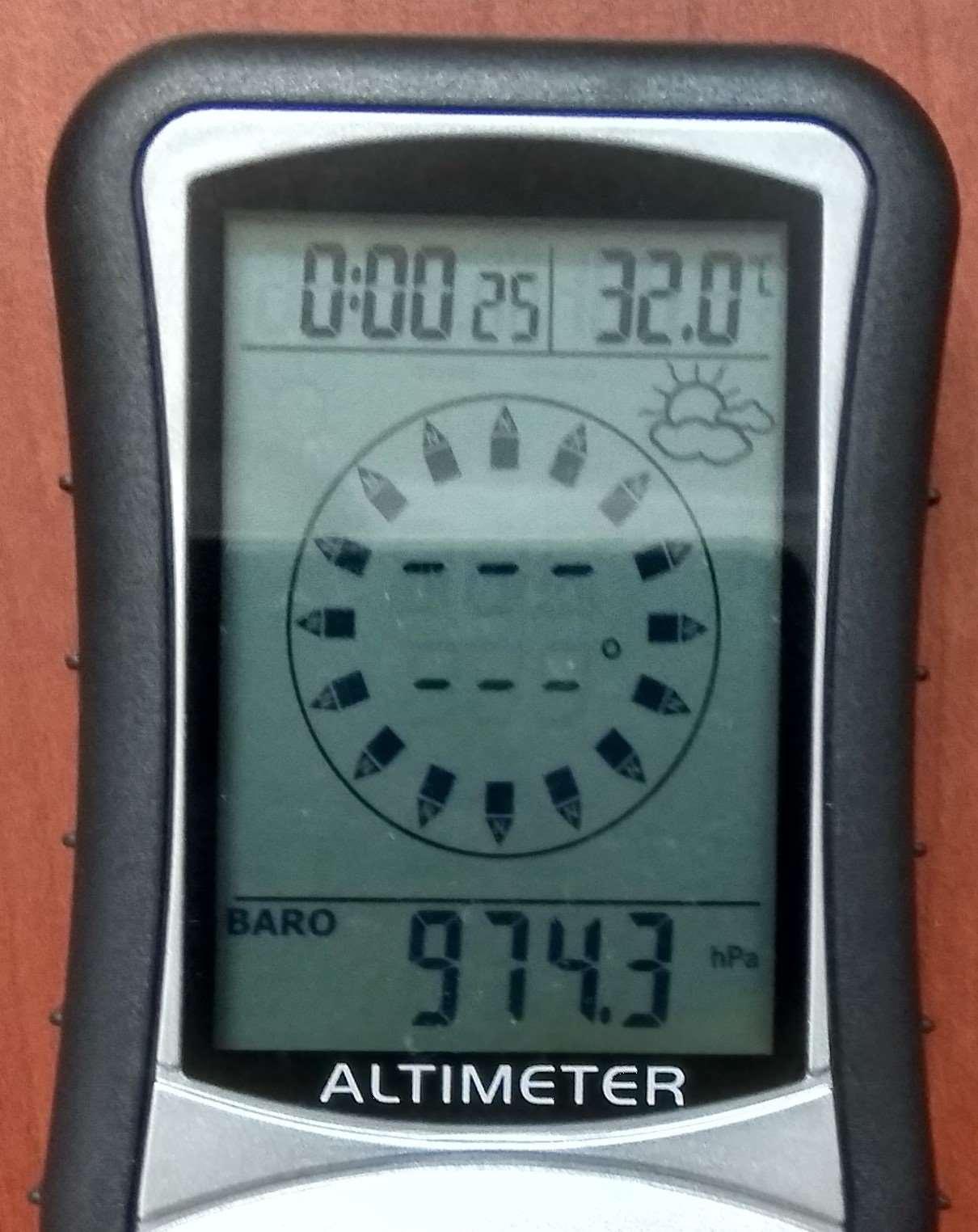

Figure1.Realtimedatameasuringdevices (a)Pyranometerdevice,(b)GHIsensor,(c)Anemometerdevice,(d)Barometerdevice
2.1.4.Dataloggingsystem
Usingtheabovementioneddevices;datahavebeenloggedfornecessaryexperiment.Figure2shows theblocklayoutofthedataloggingsystem.Hence,focusingonthemeasuredparameters;throughanemometer deviceconnectedtotwodifferentprobes(humidityandtemperatureprobe,windspeedprobe)various meteorologicalparameterslikewindspeedinm/sandkm/hr,temperaturein°Cand°Fandhumidityin percentagecanbelogged.ThedevicestoresthedatainanexternalSDcardthroughwhichthedataintheform ofMicrosoftexcelsheetcanbetransferredtothelaptopmemory.
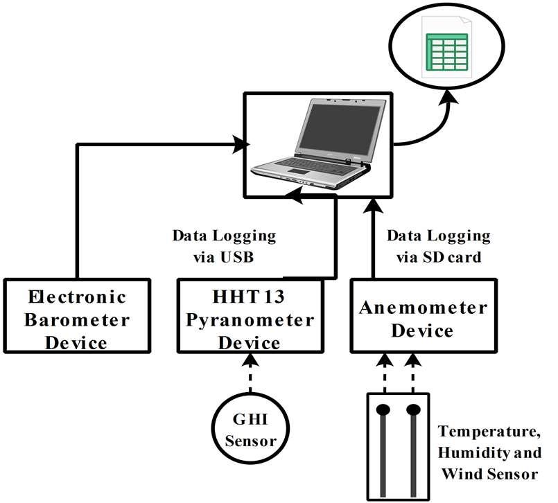
Figure2.Blockdiagramofdataloggingsystem
Theatmosphericpressurehasbeenmeasuredbytheelectronicbarometerdevice.Theothermajor parameteristhesolarirradiancewhichismeasuredusingthePyranometerdeviceandGHIsensor.Pyranometer deviceconnectedviaUSBcabletothepersonallaptopthroughhandheldterminalsoftware(HHT-13)hasbeen wellutilizedtodownloadtherecordeddataofsolarirradianceinW/m2.Thus,basedontheabovelayoutof dataloggingsystem,TableA1(submittedassupplementarysheet)showsthesetofloggeddatameasuredat thesetlocationofPatiala,Punjab,India(30.356008,76.372142).Thedatahavebeenmeasuredusingtheabove discusseddevices(Anemometer,BarometerandPyranometer).Thetableshows,therecordedvalueofrelative temperaturein°C,relativehumidityin%,thewindspeedinm/second,atmosphericpressureattheset geographicallocationinhectopascals(hpa)andthesolarirradianceinW/m2.Itistobenotedthatthedatais collectedintherealtimewith1minuteinterval,whereasherearandomsamplesetofdatahasbeengivenfor the3differentdaysforwhichdataaremeasured.
Int.J.ofAdv.inAppl.Sci.Vol.8,No.2,June2019:125–135
ISSN:2252-8814
128
(b) (c) (d)
(a)
3.PROPOSEDMETHODOLOGY
Beinguserdefined,simpleandreliable,thefuzzylogiccanalsobetermedasthesimplifiedformof theclassicallogicsinvolvedinforecasting.Theworkingoffuzzylogicsisbasedonthenon-linearmappingof inputandoutputvariablesresultinginflexibleoutput,i.e.ruleviewerwindow,whereasmultilinearregression approachtrulydependsuponthehistoricaldataofallinputsandgivestheresultinmathematicalequations.
3.1.Highdimensionalbasedfuzzylogicapproach
Figure3showsthelayoutofthedesignedsystemwithfiveuncertainweatherbasedinputswhichare temperature,humidity,windspeed,timeofday,andatmosphericpressureanditsoutputassolarirradiance. Theinputstothesystem,i.e.uncertainparametersarefuzzifiedinrespectivemembershipfunctioninthe rangeof[0,1].
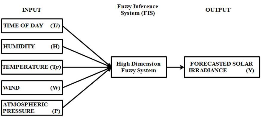
Basedontheobservedminimumandmaximumvalueforeachparameterdistributionofthelinguistic variableshasbeendone.
ThemembershipfunctionsforvariousinputsandoutputvariableisshowninFigure4,wherethe x-axispresentstheparameterdependentvalue.Forexample;dependentupontheminimumandmaximum valuesoftemperatureaxishasbeendefined,whereasthedivisionshavebeenmarkedonthebasisof observationsandlevelofvariationsinFigure4.
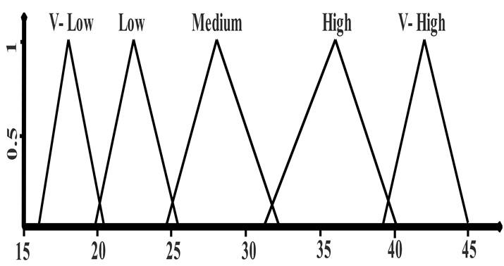
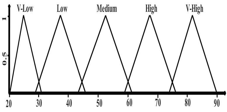
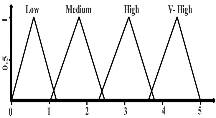
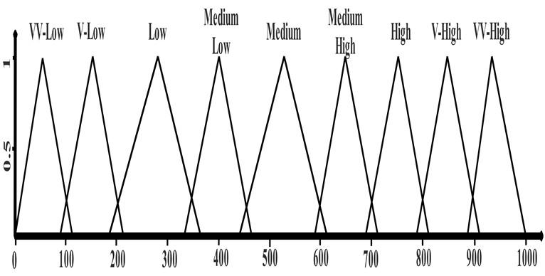
Figure4.Input/outputmembershipfunctionsfordesignedFISsystem (a)Temperature,(b)Humidity,(c)Windspeed,(d)Solarirradiance
Solarirradianceforecastingusingfuzzylogicandmultilinearregressionapproach…(SahilMehta)
Int.J.ofAdv.inAppl.Sci. ISSN:2252-8814
129
Figure3.Layoutofproposedfuzzylogicmodel(FIS)
(b) (c) (d)
(a)
The membership function of the temperature as the input given to the FIS system shown in Figure4(a)isdistributedinfivelinguisticvariables,i.e.VeryLow(VL),Low(L),Medium(M),High(H)and VeryHigh(VH).SimilartoFigure4(a),otherdependentvariables,i.e.humidityandwindspeedarementioned in Figure 4 (b) and Figure 4 (c) respectively with different number of linguistic variables. The output of the system,i.e. solarirradiancehasbeen shown in Figure 4(d).With theabove proposed system, solarirradiance isforecasteddependingupondifferentinputparameters.
3.2. Multilinear regressionapproach
Multiple linear regression model shows therelationship between multipleindependentvariables and a dependentvariable. Themathematicalmodeloftheapproachcanberepresentedas
(1)
where, y is the dependent variable, �� ,��
are k independent variables, �� is the regression coefficients and�� isrepresentedastheerrorterm.For multipleobservations,wecanwriteas
Theseequationscanberepresentedinmatrixformasfollows
(2) where,
The matrix X and y represents the historical data of all independent and dependent variables respectivelywhere asusingthe leastsquaremethod,�� of(1)canbecalculatedbythefollowing equation:
(3)
Fromaboveknownregression coefficient��,output, i.e.forecasted solar irradiancecanbecalculated fromthemultiplelinear regressionmodelasbelow:
For the measured historical data of various parameters, �� is the forecasted value of y and the difference of those two is the error in forecasting. After collecting future independent variable matrix �� , the forecasted independentvariable �� iscalculated asbelow.
Dependent upon the number of independent variables and a number of historical datasets, i.e. for a big set of data, number of rows are huge in X and y increasing the complexity in the linear regression which results in time consuming and complex solving. Hence multi-core parallel processing is used for big matrix transpose, multiplication and inverse operations which have been used in [24-26]. In the present work, five independent variables such as time of day, temperature, wind speed, humidity and atmospheric pressure and thedependentvariableastheforecastedsolarirradiance;thejobofdatahandlingandprocessinghasbeendone forreducingthecomplexityofparallelprocessing,usingtheMatlabsoftware.
ISSN:2252-8814 Int.
ofAdv.inAppl.
125–135 130
J.
Sci.Vol. 8,No.2,June2019:
��= �� +���� +�� �� +⋯+�� �� +��
,…….,
�� = �� +���� +���� +⋯+�� �� +�� �� = �� +���� +���� +⋯+�� �� +�� �� = �� +���� + �� �� +⋯+�� �� +�� �� = �� +���� +���� +⋯+�� �� +��
��
��
y= �� �� ⋮ �� ��= 1 �� �� 1 �� �� �� �� ⋮⋮⋮ 1 �� �� ⋯⋮ �� ��= �� �� ⋮ �� ��= �� �� ⋮ ��
=����+��
��
=(����) �� ��
�� =���� (4)
�� =��
�� (5)
The step by step procedure for calculating the mathematical expression between independent and dependentparametersisgivenbelow:
Step 1: MeasureandlogthedataoftheindependentanddependentvariablesanddevelopyandXmatrices. For forecasting the dependent variable, read future data of independent variables only. Calculate correlationsandexcludeunrelatedvariables.
Step 2: Use(3)toderiveregressioncoefficients�� usingMatlabsoftware.
Step 3: Forecast dependent variable using regression coefficients �� and future independent variables using(5)dependingonthe requirement.
3.3. Modelvalidationanderrorcomputation
Many methods for error calculation have been applied to the forecasting techniques for the need of evaluating the forecasted value. The most used methods include mean bias error (MBE), mean absolute error (MAE) root mean square error (RMSE), normalized root mean square error (nRMSE), mean square error (MSE)andMeanAbsolutePercentageError(MAPE)[3].Theinputforthemethodsistheforecastedvalueof the parameter at a particular time calculated using aset of data along with the other input which is the real or actualvalueoftheparameterw.r.t.thegiventime.
In the presented work, the performance evaluation of the developed fuzzy system and multilinear regression approach for forecasting of solar irradiance is determined by calculating Mean Bias Error (MBE), RootMeanSquareError(RMSE)andMeanAbsolutePercentageError(MAPE)givenby(6)to(8).
Where,Y isthepredictedortheforecastedvalueandY istheactualvaluemeasuredinrealtimeand N isthesize ofthetestdataset.The choiceofmethoddependsuponthedecisionmaker.
4. CASESTUDY,RESULTSANDERROR EVALUATION
4.1. Case study:Locationselectionanddata measurement
With the availability of various measurement devices, the real time data for 3 complete days have been monitored and logged. For the purpose of forecasting and its benefit in the planning of a microgrid, the location of TIET, Patiala (Punjab), India with longitude and latitude (30.356008, 76.372142) has been considered.Figure5showsthevariationinrecordedparameterswiththecourseoftimeandthesolarirradiance respectively.For3consecutivedays,thedatafordifferentparametersincludingrelativetemperature,humidity, wind speed, atmospheric pressure and solar irradiance were recorded using the above mentioned devices. Figure5(a)to5(c)representsthevariationintemperature,humidityandwindspeedfrommorningtoevening for3days,whereasFigure5(d)showsuncertainsolarirradiancedependentuponvariousinputparametersfor thesame time.
Int.J.ofAdv.inAppl. Sci. ISSN:2252-8814 Solar irradiance forecasting using fuzzy logic and multilinear regression approach … (Sahil
131
Mehta)
MBE= ∑[Y −Y] (6) RMSE= ∑(Y −Y) (7) MAPE= ∑ (8)
(a) (b) 0 10 20 30 40 50 13875112149186223260297334371408445482519556593630 Temperature(°C) Timesteps(10minuteinterval) Day1Day2Day3 0 20 40 60 80 100 13875112149186223260297334371408445482519556593630 Humidity(%) Timesteps(10minuteinterval) Day1Day2Day3
Timesteps(10minuteinterval) Day1Day2Day3
Timesteps(10minuteinterval)
Day1Day2Day3
Figure5.Plotforvariousparameters (a)Temperature(b)Humidity(c)Windspeed(d)Solarirradiance
4.2. Highdimensionalfuzzylogic basedapproach
Corresponding to the five input parameters; time of day, temperature, humidity, wind speed and atmospheric pressure, high dimensional fuzzy logic systems have been developed. Considering the linguistic variables of each parameter the calculated number of rules are 1200, out of which sample rules are given in Table A2 (submitted as supplementary material). For the results of the developed system, the input values: time of day- evening hours, temperature 31.6 °C, wind 2.61 m/s, humidity 41.9% and atmospheric pressure 1018.1hasbeenconsideredasshowninFigure6.
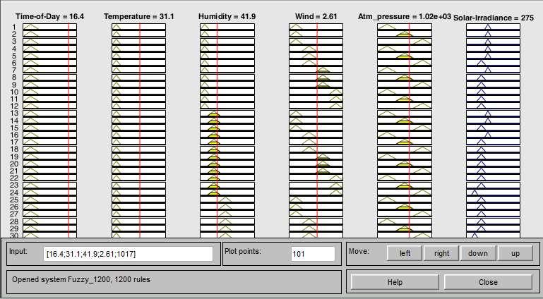
The rule viewer window for the designed high order fuzzy logic system shows the crisp value of all inputvariablesanditscorrespondingoutputi.e.forecastedsolarirradiance.Thus,theresultobtainedfromthe developed system, which is forecasted solar irradiance for a particular value of time of day, temperature, humidity, wind speed and atmospheric pressure; is given by 275 W/m2 whereas; the actual solar irradiance observedwas273W/m2
4.3. Multilinear regressionbasedforecasting
From Table 1, the (9) to (15) represents the mathematical expressions for different time intervals of theday,i.e.very shorttermtime intervalbasedforecastingrepresentedby(9)to(13) wherethe complete day has been divided into 4 time intervals; 07.00AM to 10.00AM, 10.00AM to 01.00PM, 01.00PM to 04.00PM and 04.00PM to 06.00PM. The advantage of such very short time interval is high forecasting accuracy. Also, (13) and (14) represent short term forecasting where the complete day from 07.00AM to 06.00PM has been divided in 2 intervals. Similarly (15) represents long term based forecasting expression. Figure 7 shows the forecastingresultsoftheproposedmethodologieswithboththe fuzzyandmultilinearregressionapproach.
ISSN:2252-8814 Int.
Adv.
Appl.
135 132
J.of
in
Sci.Vol. 8,No.2,June2019: 125–
(c) (d)
Figure6.Rule vieweroffuzzylogic approach
0 1 2 3 4 5 13875112149186223260297334371408445482519556593630 Wind Speed(m/s)
0 200 400 600 800 1000 1200 13875112149186223260297334371408445482519556593630 Solar
Irradiance(W/m2 )
Timeinterval
Table1.OutputofMLRapproachforvarioustimeintervals
Proposedequation
Eq.No.
7.00AM-10.00AM 6182.467+(3.763*Ti)+(2.779*Tp)+(0.978*H)-(6.139*W)-(6.16*P) (9) 10.00AM-1.00PM 2568.037+(1.12*Ti)-(0.303*Tp)-(0.686*H)-(5.725*W)-(1.911*P) (10)
1.00PM -4.00PM 141.528-(2.636*Ti)+(2.38*Tp)-(1.727*H)+(5.588*W)+(1.723*P) (11)
4.00PM -6.00PM -7435.73-(3.669*Ti)-(5.671Tp)-(2.207*H)+(3.283*W)+(9.969*P) (12)
7.00AM–1.00PM 19890+(1.553*Ti)+(16.46*Tp)-(1.441*H)+(37.121*W)-(19.684*P) (13) 1.00PM–6.00PM 1214-(2.966*Ti)+(2.011*Tp)-(1.797*H)+(22.172*W)+(0.761*P) (14) 7.00AM–6.00PM 68146.894-(1.074*Ti)+(53.995*Tp)-(5.134*H)-(1.328*W)-(67.469*P) (15)
Timesteps(10minuteinterval)
Timesteps(10minuteinterval)
Figure 7.Plotforforecastedandactualirradiance (a)Actualvs. Fuzzyoutput(b)Actualvs.MLRVeryshortintervaloutput (c)Actualvs.MLRshortintervaloutput(d)Actualvs.MLRlong intervaloutput
Figure 7 (a) represents the plot for the fuzzy logic based model with the actual output, i.e. solar irradiance, Figure 7 (b), Figure 7 (c) and Figure 7 (d) shows the results for the multilinear based forecasting approach. The analysis of the results shows almost overlapped plots for the fuzzy based system (Figure 7a); whereas with an increase in the time interval of forecasting, the variation between actual and forecasted irradianceincreases,comparedtoFigure7(b),asshowninFigure 7(d).
4.4. Error evaluation
Using(6)to(8),erroranalysisintheproposedfuzzylogicsystemandmultilinearregressionapproach hasbeenpresentedinTable2.
Table2. Errorevaluationofproposedmethodologies
Solar irradiance forecasting using fuzzy logic and multilinear regression approach … (Sahil Mehta)
Int.J.ofAdv.inAppl. Sci. ISSN:2252-8814
133
(c) (d)
(a) (b)
Error evaluation Proposedmethodology Fuzzy MLREQ. 9 MLREQ. 10 MLREQ. 11 MLREQ. 12 MLREQ. 13 MLREQ. 14 MLREQ. 14 MBE -1.395 -0.910 6.950 16.028 3.316 10.806 0.158 0.690 RMSE 10.011 28.258 26.236 32.786 29.166 50.003 31.048 104.671 MAPE(%) 1.703 10.536 2.583 3.952 14.746 12.461 8.194 22.710 0 200 400 600 800 1000 1200 11325374961738597109121133145157169181193 Solar Irradiance(W/m2)
ActualIrradianceFuzzyForecasted 0 500 1000 1500 11325374961738597109121133145157169181193 Solar Irradiance(W/m2 )
ActualIrradiance 0 500 1000 1500 114274053667992105118131144157170183196 Solar Irradiance(W/m2 )
ActualIrradiance -500 0 500 1000 1500 11325374961738597109121133145157169181193 Solar Irradiance(W/m2 )
Timesteps(10minuteinterval)
Timesteps(10minuteinterval)
ActualIrradianceMLRforecastedLongTerm
The results show very low RMSE and MAPE error in the flexible fuzzy approach in comparison to themultilinearregression approach.Also,dividingthe totaltime ofthedayinvarioustimeintervals,i.e. very short term (MLR EQ. 9 to MLR EQ. 12), short term (MLR EQ. 13, MLR EQ. 14) and long term interval (MLR EQ. 15); the analysis shows less error in very short term based forecasting compared to long term forecasting. Thus, the future work will focus on the expansion of fuzzy logic in the forecasting of renewable energysourcesandcomparingitwithanartificialneuralnetworkapproachtakingallthebasicmeteorological parametersinconsideration.
4.5.
Power calculation
For the purposeof calculatingthe poweroutput of solarPV array,(9) showstherelationbetween all the major parameters, i.e. at both Standard Test Condition (STC) and the forecasted irradiance[27,28].
P , =Y f , [1+α (T −T )] (9)
Where,P , isforecastedpoweroutputinkW,Y istheratedcapacityofthePVarray,i.e.thepower output of the panel under standard test conditionsin kW, f is the derating factor of the system in %, G , is the forecasted solar irradiance at time T in kW/m2 , G , is solar irradiance at STC (1000 W/m2), α is the temperature coefficient of power in %/°C, T andT represents the cell temperature and reference temperaturein°C.
Basedon(9),Figure8showsthecomparisonplotofpoweroutputfordifferentcaseswhichare;actual irradiance, fuzzy forecasted irradiance and MLR forecasted irradiance. As per the rated standard test conditions, Y is taken as 25kW, f is taken as 0.66, T is taken as 25 °C and temperature coefficient of poweri.e.α as0.0167.
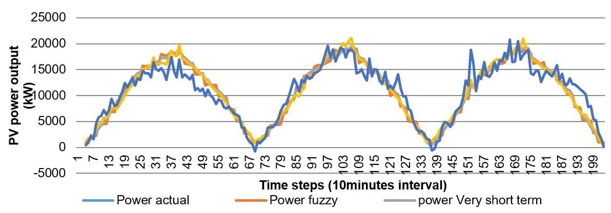
5. CONCLUSION
In this paper, considering relative temperature, relative humidity, wind speed, time of the day and atmospheric pressure as independent uncertain input variables, a high dimensional fuzzy logic system along with multilinear regression approach for short term solar irradiance forecasting has been proposed. For the purpose of real time data measurement of parameters at the set location, i.e. 30.356008, 76.372142 at the Library lawns, Thapar Institute of Engineering and Technology, Patiala (India), various devices like Pyranometer,anemometerandbarometerdeviceshavebeenused.Theresultsoftheproposedfuzzylogicbased system dependent upon the designed rule base of 1200 rules show crisp value for forecasted solar irradiance with an error of 10.011 RMSE and 1.703% MAPE in comparison to the real time observed solar irradiance. For the multilinear regression based approach, different mathematical equations dependent upon the time intervals have been produced, which shows the least error in case of very short term forecasting. Comparing theerroranalysisofmultilinearregressionbasedapproachwiththefuzzylogicbasedapproachshowsthelater to be more acceptable. Thus, depending on the forecasted values of solar irradiance and the standard test conditionsofsolarpanel,solarenergygenerationandthevariationspresentinithasbeenshown.
REFERENCES
[1] E.Lorenz,T.Scheidsteger,J.Hurka,D.Heinemann,andC.Kurz,"RegionalPVpowerpredictionforimprovedgrid integration," Progress in Photovoltaics: Research and Applications,vol.19,no.7,pp.757–771,2011.
ISSN:2252-8814 Int.J.ofAdv.inAppl. Sci.Vol. 8,No.2,June2019: 125–135 134
Figure8.Plotforforecastedpower(dependentupon actual,fuzzyandMLRsolarirradiance)
Int.J.ofAdv.inAppl. Sci. ISSN:2252-8814
[2] S. Chakraborty, M. D. Weiss, and M. G. Simoes, "Distributed intelligent energy management system for a singlephasehigh-frequencyACmicrogrid," IEEE Transaction on Industrial Electronics,vol.54,no.1,pp.97–109,2007.
[3] D. Neves, M. C. Brito, and C. A. Silva, "Impact of solar and wind forecast uncertainties on demand response of isolatedmicrogrids," Renewable Energy,vol.87,pp.1003–1015,2016.
[4] E. Duverger, C. Penin, P. Alexandre, F. Thiery, D. Gachon, and T. Talbert, "Irradiance forecasting for microgrid energy management," 2017 IEEE PES Innovative Smart Grid Technologies Conference Europe (ISGT-Europe), Torino,pp.1-6,2017.
[5] E.Corsetti,A.Guagliardi,andC.Sandroni,"Recurrentneuralnetworksforveryshorttermenergyresourceplanning in a microgrid," Mediterranean Conference on Power Generation, Transmission, Distribution and Energy Conversion (MedPower 2016),Belgrade,pp.1-9, 2016.
[6] A. Shakya et al., "Solar Irradiance Forecasting in Remote Microgrids Using Markov Switching Model," in IEEE Transactions on Sustainable Energy,vol.8,no.3,pp.895-905, 2017.
[7] R.Darbali-Zamora,C.J.Gómez-Mendez,E.I.Ortiz-Rivera,H.Li,andJ.Wang,"Solarirradiancepredictionmodel based on a statistical approach for microgrid applications," 2015 IEEE 42nd Photovoltaic Specialist Conference (PVSC),NewOrleans,LA,pp.1-6,2015.
[8] S. I. Sulaiman, T. K. Abdul Rahman, I. Musirin, and S. Shaari, "Artificial neural network versus linear regression for predicting Grid-Connected Photovoltaic system output," 2012 IEEE International Conference on Cyber Technology in Automation, Control, and Intelligent Systems (CYBER),Bangkok,pp.170-174,2012.
[9] A. D. Orjuela-Cañón, J. Hernández, and C. R.Rivero, "Very short term forecasting in global solar irradiance using linearandnonlinearmodels," 2017IEEEWorkshoponPowerElectronicsandPowerQualityApplications(PEPQA), Bogota,pp.1-5,2017.
[10] K.R.M.Supapo,R.V.M.Santiago,andM.C.Pacis,"ElectricloaddemandforecastingforAborlan-Narra-Quezon distributiongridinPalawanusingmultiplelinearregression," 2017IEEE9thInternationalConferenceonHumanoid, Nanotechnology, Information Technology,Communicationand Control,Environmentand Management (HNICEM), Manila,pp.1-6,2017.
[11] Y. Saber and A. K. M. R. Alam, "Short term load forecasting using multiple linear regression for big data," 2017 IEEE Symposium Series on Computational Intelligence (SSCI),Honolulu,HI,pp.1-6,2017.
[12] N. Jaisumroum and J. Teeravaraprug, "Forecasting uncertainty of Thailand's electricity consumption compare with using artificial neural network and multiple linear regression methods," 12th IEEE Conference on Industrial Electronics and Applications (ICIEA),SiemReap,pp.308-313,2017.
[13] XiangyunQingandYugangNiu,"Hourlyday-aheadsolarirradiancepredictionusing weatherforecastsbyLSTM," Energy,vol.148,Pp.461-468,2018.
[14] O.Ceylan,M.Starke,P.Irminger,B.Ollis,andK.Tomsovic,"Aregressionbasedhourlydayaheadsolarirradiance forecasting model by labview using cloud cover data,” in International Conference on Electrical and Electronics Engineering (ELECO),Bursa,pp.406-410,2015.
[15] M.Abuellaand B.Chowdhury,"Solarpowerprobabilisticforecastingbyusingmultiplelinear regressionanalysis," Southeast Con 2015,FortLauderdale,FL,pp.1-5,2015.
[16] U. Nalina, V. Prema, K. Smitha, and K. U. Rao, "Multivariate regression for prediction of solar irradiance," International Conference on Data Science & Engineering (ICDSE),Kochi,pp.177-181,2014.
[17] L. Suganthi, S. Iniyan, and A. A. Samuel, "Applications of fuzzy logic in renewable energy systems – A review," Renewable Sustainable Energy Reviews,vol.48,pp.585–607,2015.
[18] S. X. Chen, H. B. Gooi, and M. Q. Wang, "Solar radiation forecast based on fuzzy logic and neural networks", Renewable Energy,vol.60,pp.195-201,2013.
[19] R.S.BoataandP.Gravila,"Functionalfuzzyapproachforforecastingdailyglobalsolarirradiation,”in Atmospheric Research,vol.112,pp.79–88,2012.
[20] M.Rizwan,M.Jamil,S.Kirmani,andD.P.Kothari,"FuzzyLogicbasedModellingandEstimationofGlobalSolar EnergyusingMeteorologicalParameters,"in Energy,vol.70,pp.685-691,2014.
[21] A.Chugh,P.Chaudhary,andM.Rizwan,"Fuzzylogicapproachforshorttermsolarenergyforecasting,"in Annual IEEE India Conference (INDICON),NewDelhi,pp.1-6,2015.
[22] M. B. Mbarek and R. Feki, "Using fuzzy logic to renewable energy forecasting: a case study of France", in International Journal of Energy Technology and Policy,vol.12,no. 4,pp.357-376,2016.
[23] D. Saez, F. Avila, D. Olivares, C. Canizares, and L. Marin, "Fuzzy prediction interval models for forecasting renewableresourcesand loadsinmicrogrids,"in IEEE Transactions on Smart Grid,vol.6,no.2,pp.548-55,2015.
[24] H. S. Hippert, C. E. Pedreira, and R. C. Souza, "Neural networks for short-term load forecasting: a review and evaluation,"in IEEE Transactions on Power Systems,vol.16,no.1,pp.44-55,2001.
[25] C. Y. Tee, J. B. Cardell, and G. W. Ellis, "Short-term load forecasting using artificial neural networks," in North American Power Symposium,Starkville,MS,USA,pp.1-6,2009.
[26] K.Liu etal.,"Comparisonofveryshort-termloadforecastingtechniques,"in IEEE Transactionson Power Systems, vol.11,no.2,pp.877-882,1996.
[27] S.ArshdeepandP.Basak."ThepresentenergyscenarioandneedofmicrogridinIndia," Foundations and Frontiers in Computer, Communication and Electrical Engineering: Proceedings of the 3rd International Conference, India, pp.313-317,2016.
[28] Q.Deng,X. Gao,H.Zhou,W.Hu, "Systemmodelingandoptimizationofmicrogridusinggeneticalgorithm,"2011 2nd International Conference on Intelligent Control and Information Processing,Harbin,pp.540-544,2011.
Solar irradiance forecasting using fuzzy logic and multilinear regression approach … (Sahil Mehta)
135
InternationalJournalofAdvancesinAppliedSciences(IJAAS) Vol.8,No.2, June2019,pp.136~142
ISSN:2252-8814,DOI:10.11591/ijaas.v8.i2.pp136-142
Solarpanelmonitoringandenergypredictionfor smartsolarsystem
Isha M.Shirbhate,SunitaS.Barve SchoolofComputerEngineering&Technology, MITAcademyofEngineering,IndiaArticleInfo
Article history:
ReceivedSep12,2018
RevisedApr5,2019
Accepted May5,2019
Keywords:
Internetof things(IoT)
Prediction
Solarenergy
Solarradiation
Time-series
ABSTRACT
Solar Energy is established as an alternative source of energy known as renewableenergy.In adeveloping countrylikeIndia,theperspectiveofSolar Energy is important, as it supports a limitless source of energy. Monitoring and prediction of photo-voltaic energy generation help to reduce the energy loss and empower to utilize more energy. Solar energy prediction is challenging as it depends on the fluctuating solar radiations and climate conditions. The problem statement is to monitor solar panels and predict energy generation for energy management procedure. In this paper, the Internet of Things and Machine Learning algorithms are used as a powerful tool for developing a smart solar system. The metro-logical data such as humidity,temperatureand photovoltaicpaneldataisused asinputto forecast solarpowergeneration.Forprediction,weexaminetime-seriesofsolarenergy data with Hidden Markov Model. This model considers the probabilistic correlationbetweenpreviousvaluestonextvalueintime-series.Experimental resultsshowsthatindividualpaneldeadstateislocatedsuccessfullyandtimeseriesbasedsolarenergypredictionemulatetheactualpowergeneration.
Copyright © 2019 Institute of Advanced Engineering and Science. All rights reserved.
Corresponding Author:
IshaM.Shirbhate, SchoolofComputerEngineering&Technology, MITAcademyofEngineering, Alandi, Pune,Maharashtra,India. Email:shirbhate.isha@gmail.com.in
1. INTRODUCTION
Solar energy is thebest promising natural-renewable energy source for a green future, it has a lesser ecological impact as compared to other usual energy sources. Oil, Coal, Gases are conventional but nonrenewable sources of energy, they will run out verysoon if exploited athuge scale. Moreover, the burning of these fossil fuels increases the concentration of greenhouse gases results in global warming [1]. Solar energy does not affect greenhouse atmosphere. Currently, photovoltaic (PV) solar energy characterizes as the thirdlargest sourceof renewable energy subsequentto hydro and wind [2]. The globalinvestment in photo-voltaic solarsystemsincreasedbecauseoftransformationinfavorablegovernmentpoliciesandareductioninthecost of the PV component. These aspects give rewards for investment in solar systems which is more motivating. PV system faces some problems after installation like dirty surface, damaged connections, and junction box failureresultsin areductioninall-oversystemperformance.
IoT is a topology of the linked smart sensors and software that allows the things to assemble and transmitdatausingtheinternet.IoTbasedapplianceisverysupportiveformonitoringthesystematcheapcost. Solar panel's energy is affected by environmental conditions. Using sensors we can directly collect details aboutenvironmentalconditionslikehumidityandtemperatureofthatlocation[3-4].Thereal-timemonitoring systemusingIoTshowsthecurrentstatusofgeneratedenergy,humidity,temperature,afaultatthepanellevel anddetailsofdeadpanels[5].Adefectcanbedetectedbycollectingandanalyzingeachsensor'sdata.Electrical parameters observation generally creates a huge quantity of data. The collected data used by artificial
Journal homepage: http://iaescore.com/online/index.php/IJAAS
136
intelligence for power forecasting principles [6]. Electrical solar power production is decentralized in nature andit'sdifficulttomonitoralargeamountofdata[7].Real-timeresearchofsolarsystemisaverycomplicated task,asitdemandsaprecisePVemulatorthatmayspecificallyreproducethenon-linearcharacterofPVcells. It also conflicts realization cost, accuracy, efficiency, complexity, sensitivity with varying environmental conditions[8]. According to author Arun G.Phadkeet[9] by WideArea Monitoring (WAM),itispossible to assemble dimensions remotely from different places of power systems. Monitoring PV panels perform supervision along with faultrecognition.The faultfindingprocessassists for the recognizing diagnosisof the solarplantsystem, whichdependsonthestudyofvoltage andcurrentfactorsanticipatedfrommonitoreddata of a PV [10]. This facilities improves WAM to modern energy system protection. The proper management meetsanewschemewhichgivesanadvanceresultoftheadaptivesystem.
To develop a smartsolar plantsystem, it isessential to getaccurate PV powerforecastingresults for efficient energy management. The messy nature of ecological conditions and the surprising weather circumstances makes accurate solar power prediction enormously difficult [11]. Prediction of solar power is straightforwardly connected to the weather predictions. To make well-organized consumption of energy system,itishelpfultoforecastthereportsofsolarenergygeneration.Theexactforecastingofsolarirradiance digression enhances the quality of progression with civilizing PV energy supervision circumstances [12]. Maximum Power Point Tracking (MPPT) for solar systems assist prediction by measuring and estimating voltage and current. The Adaptive Neuro-Fuzzy (ANFIS) model utilizes PV cells temperature and solar radiation with a wavelet denoising model to obtain filtered constraints. MATLAB is easy to revise the processingoftheMPPT [13].
Theproblemstatementoftheproposedsystemistomonitorsolarpanelsandpredictthefutureenergy generation using Hidden Markov Model algorithm for energy management in IoT base environments. The objectivesoftheproposedsystemareasfollows:todevelopareal-timesolarpanelmonitoringsystemformore energyutilization;andtodevelopapredictionmodelforsolarenergymanagementprocedure.
2. SYSTEMARCHITECTURE
The proposed smart solar system starts with monitoring panel level PV plant. The solar energy monitoringsystemisimplementedbyusingIOT.Figure1showsthesystemarchitectureofaproposedsystem. We can observe the solar panel and multiple sensors and PV panels are connected with the middleware electronic board that is Raspberry Pi 3. That board is a central observing structure which collects data from sensors.Atemperatureandhumidity ofthelocationaresensed bysensorsandpowervaluesaresensedbyPV panel.Monitoringsystemdisplaysthecurrentstatusoftemperature,humidityandgeneratingenergypowerat certain timeintervals.Thesystemdisplaysthe entireinformationonthewebpagesandsubsequently,itstores data on thecloud.

Int.J.ofAdv.inAppl. Sci. ISSN:2252-8814
panel monitoring and energy prediction for smart solar system
137
Solar
(Isha M. Shirbhate)
Figure1.Architecturediagramofproposedsystem
Prediction system works on historical data of solar power collected by monitoring system. To make advance adaptive forecast system we apply a Hidden Markov Model (HMM) which works as time-series prediction. The system states definition and transition probabilities for constructing HMM. The proposed methodgivesanaccurate predictionof solar energygeneration.
3. RESEARCH METHOD
3.1. Monitoringsystem
The monitoring system measure and display the collected data by sensors and solar panels. We monitored temperature, humidity and generating solar power using smart devices. It is essential for a monitoringsystemthatthecustomersmustknowthepotentialandpracticalboundariesofdevices,operational deviations and objective of data analysis. As we know python is a largely used, advanced, interpreted, highlevel, dynamic programming language, so we use python programming to complete this task. Monitoring constraintsarethenuploaded on thecloudusing apython program.Flask worksas a light-weightframework, which is written in Python. The Flask uses stretchy cast off to read the sensor values. We consider the DHT11sensorthatshowstemperaturewithhumidityasweatherinformation fromreal-timesituations.Thesystem canworkonthemultiplesolarpanelswhichhadtheheterogeneousconfiguration.
3.2. Predictionsystem
Intheproposedsystem,weworkonHMMforfindingthemostprobabletime-series.Thetime-series prediction is calculated by estimating probability of state transition and observation sequences for the predetermined state which gives precision in prediction. This method takes historical records of power as a input. Markov chain property says that the possibility of every subsequent state depends just on earlier state [14,15].TheHMMhave��states,knownas�� ,�� ,…,�� wherediscretetime-period�� =0,1,…Oneachtimeperiod, the system is in the state which is freely available called �� states. These states with time �� is identify like�� , by �� ∈ {�� ,�� ,…,�� }. At each and every time-period, the state �� form, one resulting symbol accordingtoObservation andEmissionProbabilitiesallocation.
We find hidden and observed states called as a state probability vector��, inter-state transition probability matrix �� and emission probability matrix ��. Markov chain can translate calculated data to the variousstates, sothe seriesofenergygeneration valuesistranslatedintothenumberofstates. Therefore,Statetransitionprobabilitiesare{�� ,�� ,…,�� } Itsignifiesprobabilityofonestate toanotherstate asastatetransitionprobabilitymatrix
��= �� ,�� = Р(��|��)
Here, �� representsa number of rows and �� number of columns. The observation probability allocation signify forstate�� is����,�� = 1,….,�� inthestate��
��= ��(�� ) ,����(�� )= Р(�� |��)
Asquantityof symbolsaretwo thus�� = 2 Withvectorinitialprobabilitymatrix
Π=(Π),Π =Р(��)
Atlast,Modelisshown by��=(��,��,Π).
The purpose of energy prediction is examining a Hidden Markov Model by considering observed time- series. Maximum likelihood estimation method estimate��∗ which maximizes a likelihood of training series, ������={������} for improvement in Р(������|��). Autonomous and supremely spotted samples of, ������={������} are anxious from the probability allocation Р(������|��).The objective is to get a value of �� whichoriginates������ toР(������|��)aslikelyasprobable.
������ ≅Р(������|��)
Theprobabilityvariationmethodisprecise withidentified��=(��,��,Π). Recalculate��for theentire steps with likelihood probability of frequency of state�� following state�� . This variation step is reiterate till convergenceforthetime-intervalofwhichР(������|��)notreduces.
ISSN:2252-8814 Int.J.ofAdv.inAppl. Sci.Vol. 8,No.2,June2019: 136–142 138
Steps
Algorithm
1: ObserveTime-SeriesinSequence ������={0′��,1′��}
2: Namedasdifferentobservationsymbolsforstates N ��={0,1}
3: CalculateapproximatelyvaluesofMarkovmodeltomaximizeprobabilityР(������|��) ��=(��,��,Π)
4: PredictEnergygenerationdependsonpastobservationtime-series Р(������,1|��)<Р(������,0|��)��ℎ������(��+1)=0 Р(������,1|��)≥Р(������,0|��)��ℎ������(��+1)=1
5: Producepredictedobservationtime-seriesfor��=��+1����2�� ��������={������} using{������}
The algorithm initially examines all the records from the dataset and spites every characteristic. At step 2, it mentions each attribute as a unique symbol i.e. 0��and1��. The sampling approach work with the helpofHMMmodelinstep3.Thennextwedopredictionofobservationtime-seriesofmovingratioofinput. Lastly,inconclusionstep5givesthepredictionoutput.ThisprocessiscalledasanobservableMarkovModel. It gives a set of number of states at the specific time period, where every state communicates to the next state [16]. Thus the presented model seems preventive for several problems. We can expand the idea of a Markov Model to embrace the sets while observation sequence isa probabilistic method of states. HMM is a vitalversionofMarkovmethod,yetHMMisaself-governingprocedure.Here,statescommunicatetoagroup of same probability allocation of observation. While working on this algorithm we found two challenging problemsthataremention.
3.2.1.Likelihoodproblem
The first problem is to calculate the likelihood sequence of a distinct observation sequence that is a newobservationsequenceandasetofmodels.Itfindsamodelwhichgivesthebestsequence.Thebestpossible sequencelinkedwithknownobservationsusingstatesequenceandObserved Time-Series
Р(������|��)=ΠР(������|��) ⨯ ΠР(��|�� )
We used an efficient algorithm called the forward algorithm. The forward algorithm is a kind of dynamic programming algorithm. It computes the observation probability by summing over the probabilities ofallpossiblehidden-statepathsthatcouldgeneratetheobservationsequence.
3.2.2.Decodingproblem
HMM model, which contains hidden variables, the challenge is to determine which sequence is the underlyingsourceofsomesequenceofobservations.Itiscalledthedecodingtask.Thedecoderfindsthebesthiddensequence,thisproblemsolvedbytheViterbialgorithm.Itispossibletoalterthemodelconstraints ��= (��,��,Π) for maximize Р(������|��). The Viterbi Algorithm score finest from the a particular path at initial time��observations,trimwithstate �� ,presentedas:
��(��)=������Р(�� ,�� , ,�� =��,������|��)
4. RESULTSANDDISCUSSION
Theresultsaresplitupintothreeparts.Firstpartisaperformanceevaluationofthemonitoringsystem. The second part is an analysis and comparison of the prediction model and the third part is a case-study on a proposedmethod.
4.1. A solarplantmonitoringsystem
The system shows a status dashboard of monitoring panelswith energy generation level.It monitors the temperature in degree celsius and humidity in the percentage. Solar energy differs by environmental seasons [3], Figure 2 shows graphs for hourly temperature and solar energy generation in sunny, cloudy and rainy days. The system represents graphs for analyzing the performance in a standard method to provide the understandable view of information to the users. The dashboard is accessible to the users from anywhere and anyplace.Iftheone-timeconnectiontotheserverissuccessful,thestatusofthesystemisconstantlypassedto the web server for monitoring the parameters of solar Power Conditioning Unit (PCU). We can examine the intense values generated by solar PCU. The system is able to analyze past average ratio of energy generation monthlyandyearly.In addition,thesystemalsoforecaststhe panel'sdeadstate andtheerrorfinding.
Solar panel monitoring and energy prediction for smart solar system (Isha M. Shirbhate)
Int.J.ofAdv.inAppl. Sci. ISSN:
2252-8814
139
4.2. Solarenergyprediction
We identified that the consequences of prediction are affected by the environmental situations and locationofPVplant[6].Inthepredictionmodel,weusedanadvancedHiddenMarkovModeltopredictsolar energy generation. Considering the real-time statistics measured by the monitoring system, we get better results. FollowingTable1 showsthe actualvaluesandpredictedvalues,forfewhourlysamplecases. Accurateness of prediction is calculated with help of Root Mean Square Error (RMSE) and Mean Absolute Percentage Error (MAPE). We compare the proposed algorithm with Linear Regression [17] as shown in Table 2. If rate among predicted and actual values are close to zero by RMSE, then we find betterquality output at low error. Figure 3 and Figure 4 show day wise and month-wise, actual with predicted PV powergenerationfordifferentenvironmentalconditions.
Table 1.Differentsample caseson hourlydata
Table2.Comparisonbetweenproposedmethod andanotherpredictionmethod
ISSN:2252-8814 Int.J.ofAdv.inAppl. Sci.Vol. 8,No.2,June2019: 136–142 140
(a)
(b)
Figure2.(a) Temperature and(b)Powerindifferentweatherconditions
Hour ObservationSeq States ActualOutput ProposedModel 1 1-0-1-……..0 2 1.44 1.56 2 0-1-0-.…….1 2 1.50 1.57 3 1-1-0-.…….1 2 1.82 1.67 4 0-1-1-.…….0 2 1.55 1.65
Sr.No. Method RMSE MAPE 1 ProposedMethod 0.642 8.442 2 LinearRegression 1.501 13.440
(a)
0 20 40 60 80 100 56789101112131415161718 Temperature(C) Time(Hours) SunnyRainyCloudy 0 0.5 1 1.5 56789101112131415161718 Power(W) Time(Hours) SunnyRainyCloudy 0 1 2 3 4 5 0102030 Power(W) Time(day)(a) Actual Predicted 0 1 2 3 4 5 0102030 Power(W) Time(day)(b) Actual Predicted 0 1 2 3 4 5 6 7 0102030 Power(W) Time(day)(c) Actual
Figure
3.ActualandpredictedPV powergenerationin
Cloudy,(b)Rainyand(c)Sunny month
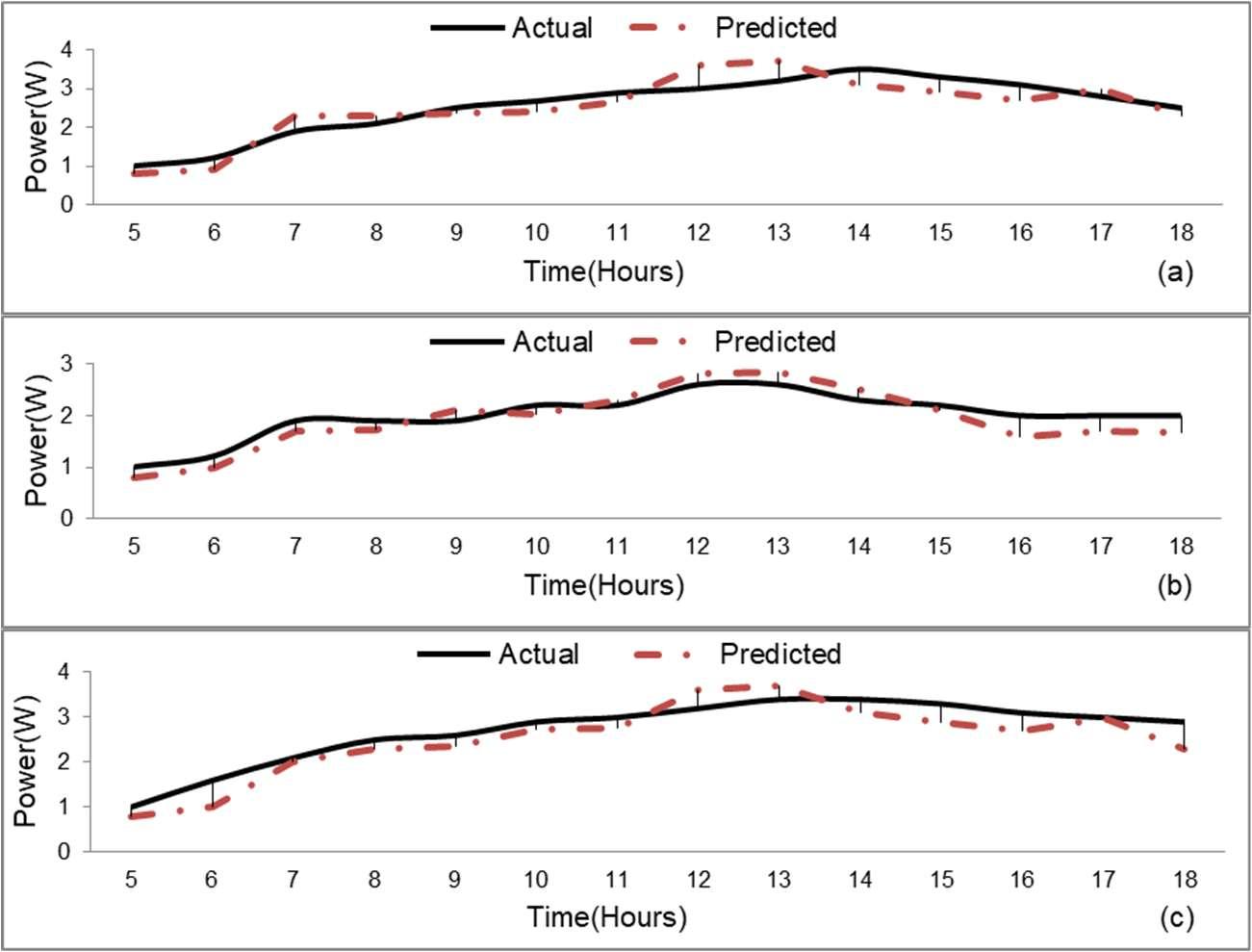
Figure4.ActualandpredictedPVpowergenerationfor(a)Cloudy,(b)Rainyand(c)Sunnyday
4.3.Casestudy
Theproposedmethodologyistestedonadatabaseofthelarge-scalesystem,whichislocatedatMIT AcademyofEngineering,Alandi,PunecampusasshowninFigure5.Therearesixdistributedsolarplants, onesinglepaneliswith315wattpeakcapacityandwholesolarsystemhavingthe435kWcapacity.Thesystem addedwithirradiancesensor,temperaturesensorandwindspeedsensorformonitoringtheweathersituations. Weconsiderthehourlypowerdataofoneplanttopredictthesolarpower.Figure6showstheactualand predictedpowergenerationofthesolarplant.

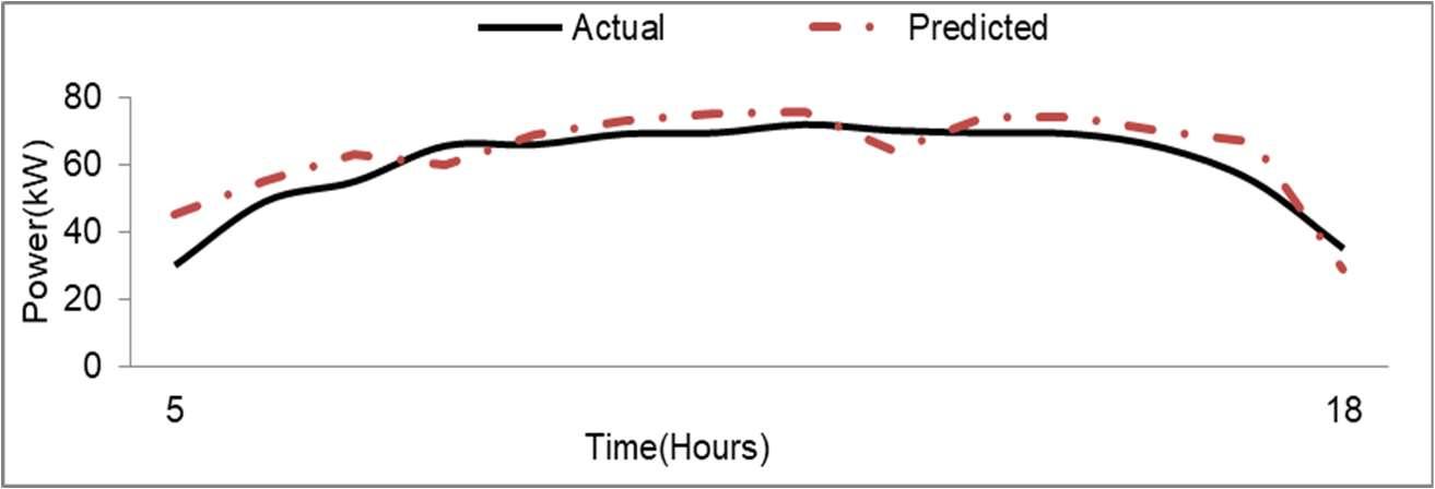
Figure6.ActualandpredictedPVpowergenerationoflarge-scalesolarplant
Solarpanelmonitoringandenergypredictionforsmartsolarsystem(IshaM.Shirbhate)
Int.J.ofAdv.inAppl.Sci. ISSN:2252-8814
141
Figure5.Large-scalesolarplantatMITAcademyofEngineering,Alandi
5. CONCLUSION
Solarenergyistrustworthyandsustainablehencetheutilizationofthissmartsolarsystemisreliable, adequate and cost-efficient. The proposed smart solar system comprises both Monitoring and Prediction. We have used the Internet of Things (IoT) for monitoring by considering parameters like Temperature, Humidity andSolarPower.InternetofThingsisprovidingpracticallyexpertmethodsthatoffersrequiredoutcome.The designed system monitors panel level PCU and anticipates the error findings. We can analyze the weekly or monthlyperformanceofpanels. On theotherhand, Prediction uses HiddenMarkov Modelforforecastingthe solar power. We have developed an hourly prediction system. Considering historical records, the proposed model is able to predict accurate power generation in time- series method. Numerical results show that the proposedmodelachievesbetterpredictionaccuracythanthesimpleLinearRegressionmodel.
REFERENCES
[1] I. Gherboudj and H. Ghedira, "Assessment of solar energy potential over the United Arab Emirates using remote sensing andweatherforecastdata," Renewable and Sustainable Energy Reviews, vol. 55:1210-1224, 2016.
[2] Moreno-Garcia, E. Palacios-Garcia, V. Pallares-Lopez, I. Santiago, M. Gonzalez-Redondo, M. Varo Martinez, and R. Real-Calvo, "Real-time monitoring system for a utility-scale photovoltaic power plant," Sensors, vol. 16(6), p.770, 2016.
[3] S. R. Madeti and S. N. Singh, "Monitoring system for photovoltaic plants: A review," Renewable and Sustainable Energy Reviews,vol.67,pp.1180-1207, 2017.
[4] B.Ando,S.Baglio,A.Pistorio,G.M. Tina,and C.Ventura,"Sentinella:Smartmonitoringofphotovoltaicsystems atpanellevel," IEEE Transactions on Instrumentation and Measurement,vol.64(8),pp.2188-2199, 2015.
[5] F. O. Hocaoglu and F. Serttas, "A novel hybrid (Mycielski-Markov) model for hourly solar radiation forecasting," Renewable Energy,vol.108,pp.635-643, 2017.
[6] S. Daliento, A. Chouder, P. Guerriero, A. M. Pavan, A. Mellit, R. Moeini, and P. Tricoli, "Monitoring, diagnosis, andpowerforecastingforphotovoltaicfields:Areview," International Journal of Photoenergy, 2017.
[7] C. Stegner, M. Dalsass, P.Luchscheider, and C. J. Brabec,"Monitoring and assessment of PV generation based on acombinationof smartmeteringand thermographicmeasurement," Solar Energy,vol.163,pp.16-24, 2018.
[8] S.Senthilkumar,G.P.C.,“HiddenMarkovModelbasedchannelselectionframeworkforcognitiveradionetwork,” Computers and Electrical Engineering,vol.65,pp.516-526, 2018.
[9] A.G.Phadke,P.Wall,L.Ding,andV.Terzija,"Improvingtheperformanceofpowersystemprotectionusingwide areamonitoringsystems," Journal of Modern Power Systems and Clean Energy,vol.4(3),pp.319-331, 2016.
[10] S. Silvestre, L. Mora-Lopez, S. Kichou, F. Sanchez-Pacheco, and M. Dominguez-Pumar, "Remote supervision and faultdetectionon OPCmonitoredPVsystems," Solar Energy, vol.137,pp.424-433, 2016.
[11] C.Wan, J. Zhao, S. Member, and Y. Song, "Photovoltaic and solar power forecasting for smart grid energy management," Journal of Power and Energy Systems,vol.1(4),pp.38-46, 2015.
[12] S. Mohanty, P. K.Patra, S. S. Sahoo, and A. Mohanty,"Forecastingof solar energy with application for a growing economy like India: Survey and implication," Renewable and Sustainable Energy Reviews, vol. 78, pp.539-553, 2017.
[13] A. Chikh and A. Chandra, "An optimal maximum power point tracking algorithm for PV systems with climatic parametersestimation," IEEE Transactions on Sustainable Energy,vol.6(2),pp. 644-652, 2015.
[14] M. J. Sanjari and H. B. Gooi, "Probabilistic forecast of pv power generation based onhigher order markov chain," IEEE Transactions on Power Systems, vol.32(4),pp.2942-2952, 2017.
[15] S. S. Barve, "Dynamic channel selection and routing through reinforcement learning in cognitive radio networks," IEEE International Conference on Computational Intelligence and Computing Research, 2012.
[16] W.J.I.LiandJinboPedrycz,"Multivariatetimeseriesanomalydetection:Aframeworkofhiddenmarkovmodels," Applied Soft Computing Journal, vol.60(27),pp.229-240, 2017.
[17] N. Sharma,P. Sharma, D.Irwin, and P. Shenoy,"Predictingsolargenerationfromweatherforecastsusing machine learning," SmartGridCommunications(SmartGridComm),2011IEEE InternationalConference,pp.528-533,2011.
ISSN:2252-8814 Int.J.ofAdv.inAppl. Sci.Vol. 8,No.2,June2019: 136–142 142
InternationalJournalofAdvancesinAppliedSciences(IJAAS) Vol.8,No.2, June2019,pp.143~153
ISSN:2252-8814,DOI:10.11591/ijaas.v8.i2.pp143-153
Performanceevaluationandcomparisonofdiodeclamped multilevelinverterandhybridinverterbasedonPDand APODmodulationtechniques
N.Susheela, P.SatishKumar DepartmentofElectricalEngineering,OsmaniaUniversity,IndiaArticleInfo
Article history:
ReceivedAug29,2018
RevisedApr1,2019
Accepted May8,2019
Keywords:
Diodeclampedmultilevel inverter
Hybridinverter
Sinusoidalpulse width modulation
Totalharmonicdistortion
ABSTRACT
The popularity of multilevel inverters have increasing over the years in various applications without use of a transformer and has many benefits.Thisworkpresentstheperformanceandcomparativeanalysis ofsinglephasediodeclampedmultilevelinverterandahybridinverter with reducednumberofcomponents.Astherearesomedrawbacksof diode clamped multilevel inverter such asrequiring higher number of components, PWM control method is complex and capacitor voltage balancingproblem,animplementationof hybridinverterthatrequires fewer components and less carrier signals when compared to conventional multilevel inverters is discussed. The performance of single phase diode clamped multilevel inverter and hybrid multilevel inverter for seven, nine and eleven levels is performed using phase disposition, alternate phase opposition disposition sinusoidal pulse width modulation techniques. Both the multilevel inverter are implemented for the abovementioned multicarrier based Pulse Width Modulation methods for R and R-L loads. The total harmonic distortion is evaluated at various modulation indices. The analysis of the multilevel inverters is done by simulation in matlab/simulinkenvironment.
Copyright © 2019 Institute of Advanced Engineering and Science. All rights reserved.
Corresponding Author:
N.Susheela, DepartmentofElectricalEngineering, UniversityCollege ofEngineering, OsmaniaUniversity, Hyderabad,Telangana,India. Email:nsusheela2007@yahoo.com
1. INTRODUCTION
The multilevel inverter (MLI) is now proven technology for medium/high voltage high- power applications such as such as marine drives, variable-speed drives, reactive power compensation, steel rolling millsandotherapplications.Theconceptofpowerconversioninmultilevelinverters(MLI)istosynthesizea staircasevoltagewaveformfromseverallowervoltageDCsourceswhichapproachesthesinusoidalwavewith reduced harmonic distortion has got several advantages and have drawn tremendous interest in high power highvoltageapplications[1-4].Incaseofmultilevelinvertersthesemiconductorsarewiredtoformseriestype connection so that the operation at higher voltages is possible. The switching losses and the switching frequency can be reduced by staggering the switching because the switches are not truly series connected. Conventional multilevel inverters include neutral point clamped (diode-clamped) inverter, flying capacitor (capacitorclamped)inverterandcascadedH-bridgeinverter.Themajordrawbackofmultilevelinvertersisthe
Journal homepage: http://iaescore.com/online/index.php/IJAAS
143
highernumberofpowersemiconductorswitchesneededthatcomplicatestheoverallsystem[5-8].Usinglower rated switches in the multilevel inverter can reduce the cost of active semiconductors compared to two level inverters. Associated gate drive circuits are required for each active semiconductor which increases the complexity.In[9],thesymmetricaltopologywhichiscalledasreversingvoltagetopologyisimplementedfor single phase seven level inverter using phase disposition method. This multilevel inverter topology requires less number of components when compared to conventional multilevel inverters. A multilevel inverter with reversing voltage component has many advantages as the levels increase when compared to conventional multilevel inverters. The hybrid topology eliminates the diodesand capacitors thatare used in diode clamped inverters,capacitorsusedinflyingcapacitorinvertersandalsoreducestheswitchesandcarriersignalsrequired thanincascadedinverters,diodeclamped,andflyingcapacitorsinverters.Anapproachofutilizinghigh-power deviceswithlow-switching-frequencyreducesvoltagedistortionofoutputbuthasgotcurrentharmonicswhich isamajordrawback[10-13].Thereareasymmetricalmethodsofusingdifferentvaluesofvoltagesourcewhich requires more number of power switches and diodes with different rating. Some topologies suffer from the capacitorbalancingproblems.WhereasincaseofhybridMLI,thevoltagesourcesusedhaveequalvaluesand has many advantages compared with the methods discussed above. It utilizes less number of switches and carriersandalsooperatestheswitchingdevicesatlinefrequency.ThedifferentmulticarrierPWMmethodsare reportedtominimizetotalharmonicdistortion(THD).AdvancedMLItopologieshavebeenproposedrecently such ashybrid multilevelinverter, softswitching inverterand generalizedMLI.These areextensively used in applications like FACTS, tractions and industrial drives [14-19]. The phase disposition (PD) and alternate phase opposition disposition (APOD) sinusoidal pulse width modulation (SPWM) methods are used to drive the single phase DCMLI and hybrid MLI for different levels. The general MLI inverter structure for various levelsisshownin inFigure1.
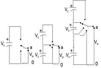
2. MULTILEVELINVERTERS
The analysis of diode clamped multilevel inverter and hybrid inverter are discussed based on sinusoidalpulsewidthmodulationtechniques.
2.1. Diode clampedMLI
In order to generate seven levels by SPWM, six carriers and a sinusoidal reference signal for modulator areneeded for DCMLI. The arrangementof thecarriersfor APODand PDtechniquescan be seen inFigure 2andFigure3.
ISSN:2252-8814 Int.J.ofAdv.inAppl. Sci.Vol. 8,No.2,June2019: 143–153 144
Figure1.MLIinverterstructurefortwo,three andn-levels
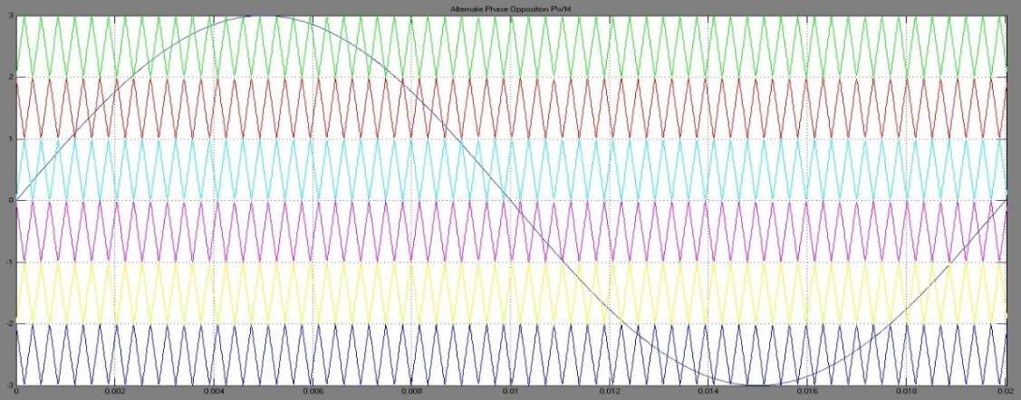
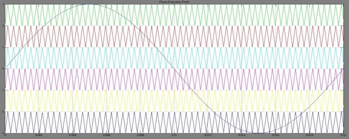
2.2.HybridMLI
ThehybridMLIhastwostagesinwhichonestageislevelgenerationandotherispolaritygeneration stage.Thefirststagerequireshigh-frequencyswitcheswhichproducestherequiredpositivelevels.Theoutput polaritycanbeobtainedbythesecondstagethathaslowfrequencyswitches.ThehybridMLIeliminateshigher numberswitchesthatarerequiredtogenerateoutputlevels.Thesinglephase7levelDCMLIusiingSPWM requires6carriers,butthreecarriersaresufficientforhybridMLI.The7levelhybridMLIrequiresonly3 carriersandasinusoidalreference.Figure4andFigure5representsthecarrierarrangementusingAPODand PDSPWMtechniques.
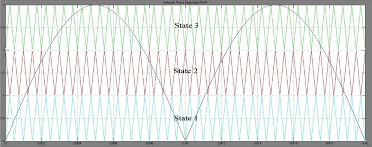
Figure4.APODPWMtechniqueforsinglephase7levelhybridinverter
Perfomanceevaluationandcomparisonofdiodeclampedmultilevelinverterbased…(N.Susheela)
Int.J.ofAdv.inAppl.Sci. ISSN:2252-8814
145
Figure2.APODPWMtechniqueforsinglephase7levelDCMLI
Figure3.PDPWMtechniqueforsinglephase7levelDCMLI
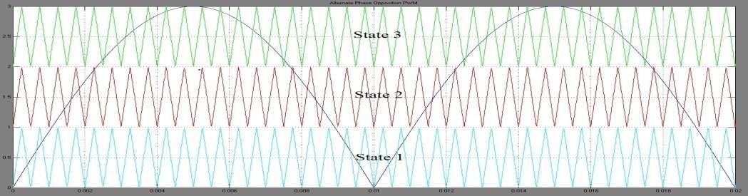
3. IMPLEMENTATIONOFDCMLIANDHYBRIDMLI
Figure 6 and Figure 7 depicts the simulation models for producing gating signals in a single phase 7 levelDCMLIusingAPODand PDSPWMtechniques.
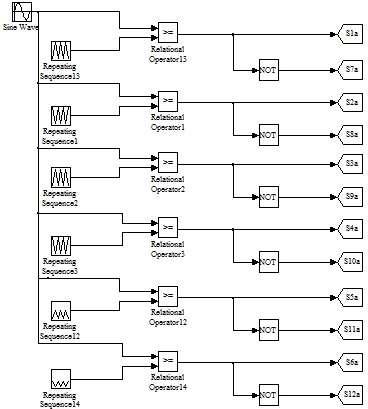
Figure6.Modelforgatingsignalsof7levelDCMLI using APODmethod
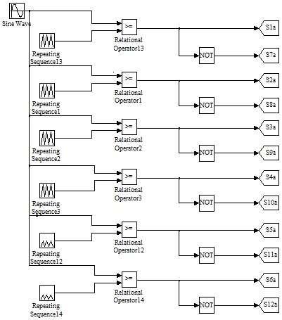
Figure7.Modelfor gatingsignalsof7level DCMLIusing PDmethod
Figure 8 shows the simulation model using APOD method for generating gating signals in level generation stage of 7 level hybrid MLI. The simulation model for producing gating signals in polarity generationstageof7levelhybridMLIisshownin Figure9.
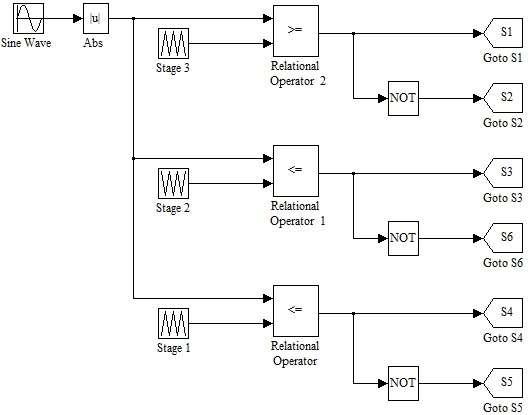
Figure 8.Modelforgatingsignalsinlevel generationpart
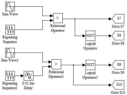
Figure 9.Modelforgatingsignalsinpolarity generationpart
ISSN:2252-8814 Int.J.ofAdv.inAppl. Sci.Vol. 8,No.2,June2019: 143–153 146
Figure5.PDPWM techniqueforsingle phase7levelhybridinverter
4. RESULTSANALYSIS
The results obtained for DCMLI and hybrid MLI are eloberated for various loads. The performance of the inverters using LC filter are also discussed. The results obtained using APOD technique is presented belowfor0.9modulationindex.
4.1. DCMLIfor7,9and11levels
The performance of DCMLI is shown below for various levels using different loads. The results of DCMLIfor7levelsaredepictedin Figure10toFigure 12.
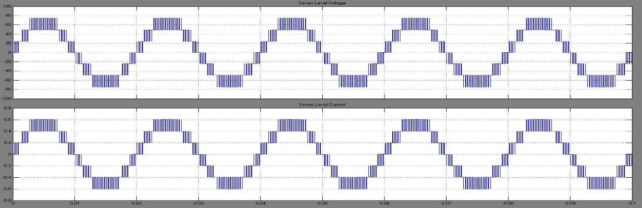
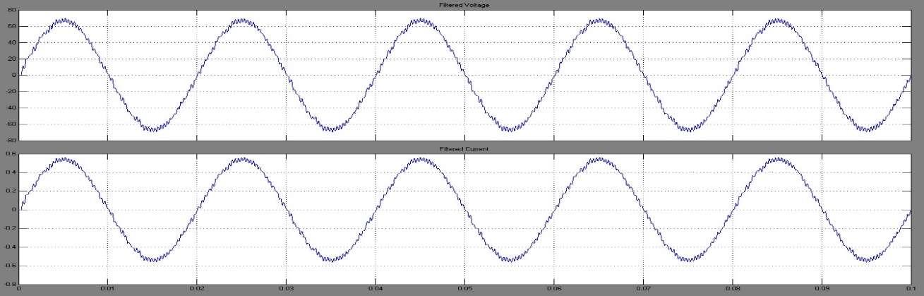
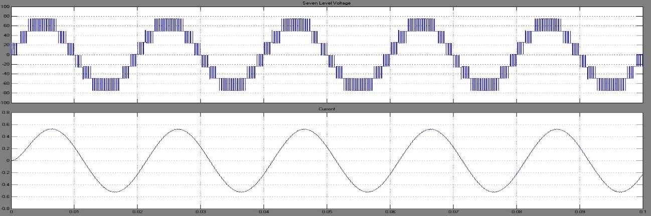
Perfomance evaluation and comparison of diode clamped multilevel inverter based… (N. Susheela)
Int.J.
Adv.inAppl. Sci. ISSN:2252-8814
of
147
Figure 10.Waveformsofvoltageandcurrentin7 levelDCMLIforRload
Figure11.Waveformsofvoltageandcurrentin7levelDCMLIforRloadwithfilter
Figure 12.Voltageand currentwaveformsof7 levelDCMLIforR-Lload
The 9 levelDCMLI results can beseen from Figure 13 to Figure15using APOD method.Figure 16 toFigure 18presentstheresultsofDCMLIfor 11levels.
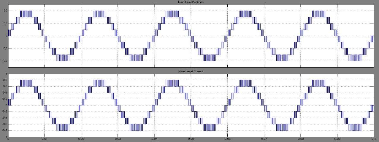
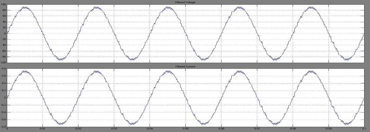
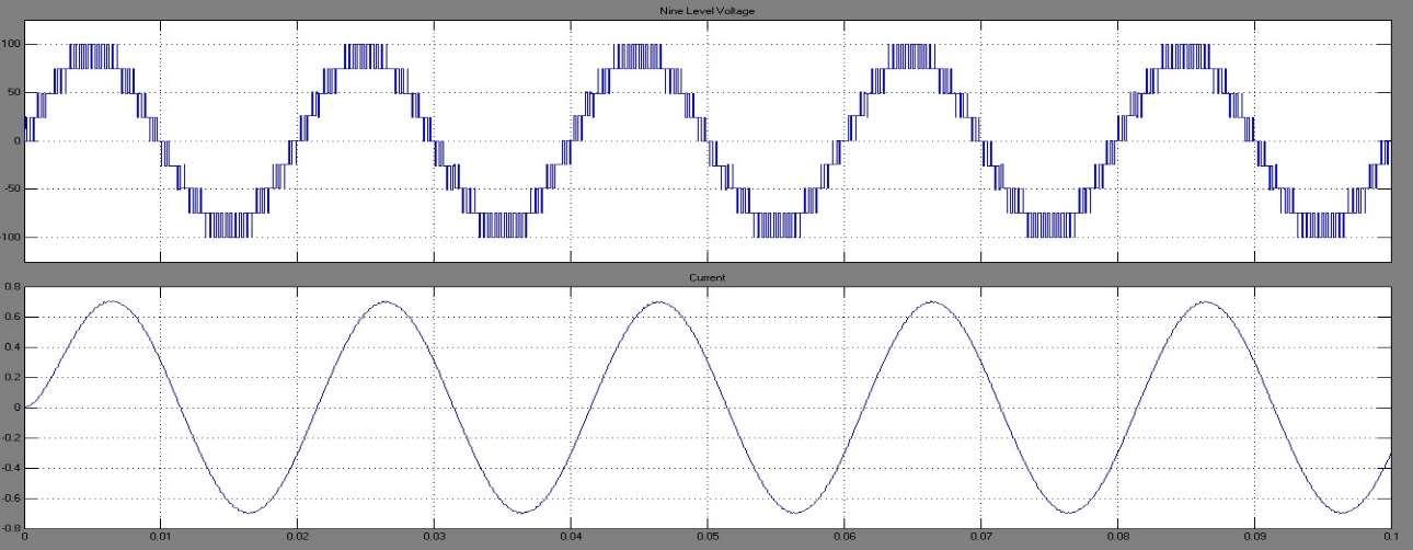
ISSN:2252-8814 Int.J.ofAdv.inAppl. Sci.Vol. 8,No.2,June2019: 143–153 148
Figure 13.Waveformsofvoltageandcurrentin9 levelDCMLIforRload
Figure14.Waveformsofvoltageandcurrentin9levelDCMLIforRloadwithfilter
Figure15.Waveformsofvoltage andcurrentin9levelDCMLIforR-Lload
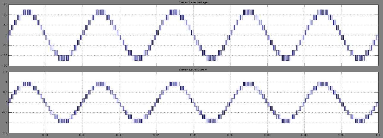
16.Waveformsofvoltageandcurrentin 11levelDCMLIforRload
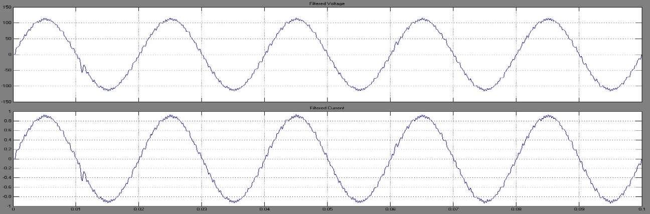
17.Waveformsofvoltageand currentin11levelDCMLIforRloadwithfilter
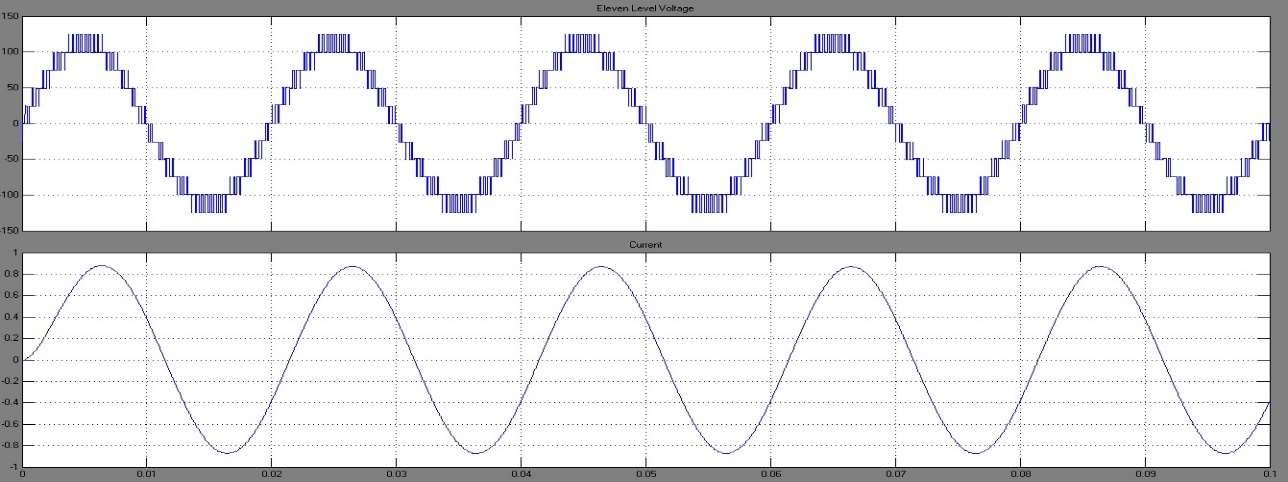
18.Waveformsofvoltageand currentin11levelDCMLIforR-Lload
4.2. HybridMLIfor7, 9and11levels
The performance of hybrid MLI are presented in this section for various levels at different loads. Figure 19 to Figure 21 shows the results for single phase 7 level hybrid MLI. Whereas the results for single phase 9 level hybrid MLI are shown from Figure 22 to Figure 24. The waveforms obtained for single phase hybridMLIareshownfromFigure25 toFigure27for11levels.
Perfomance evaluation and comparison of diode clamped multilevel inverter based… (N. Susheela)
Int.J.ofAdv.inAppl. Sci. ISSN:2252-8814
149
Figure
Figure
Figure
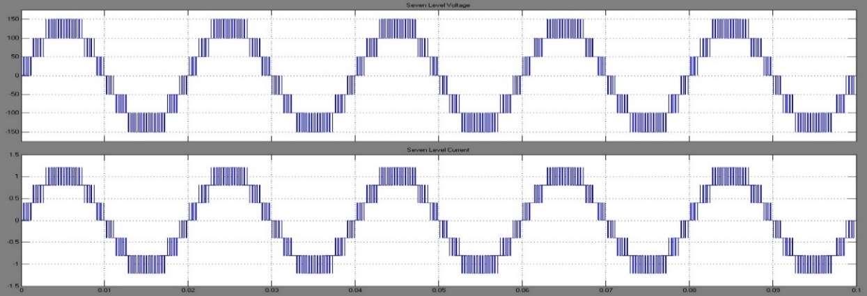
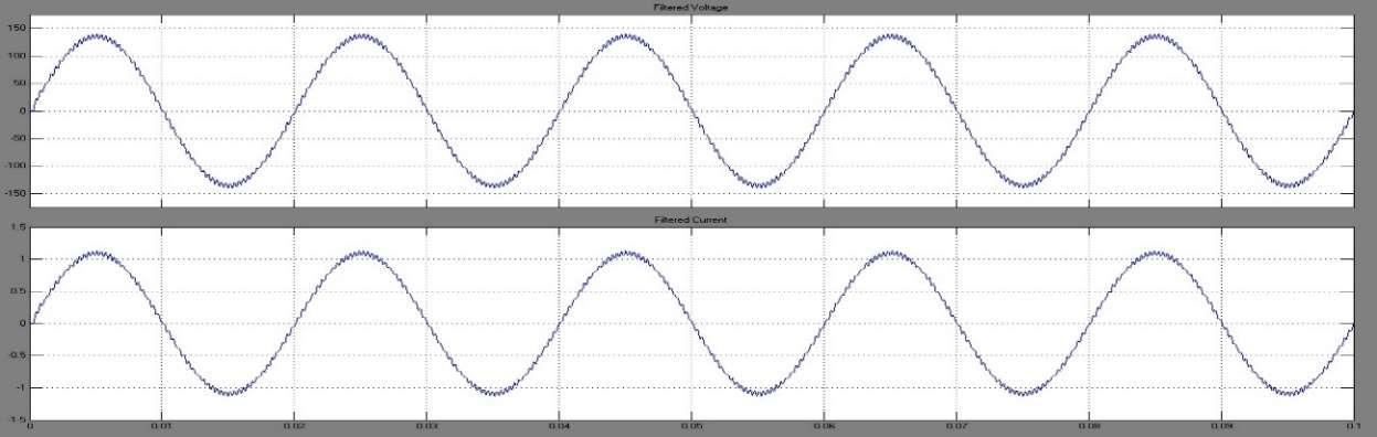
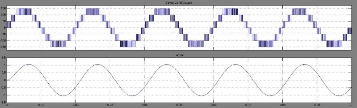
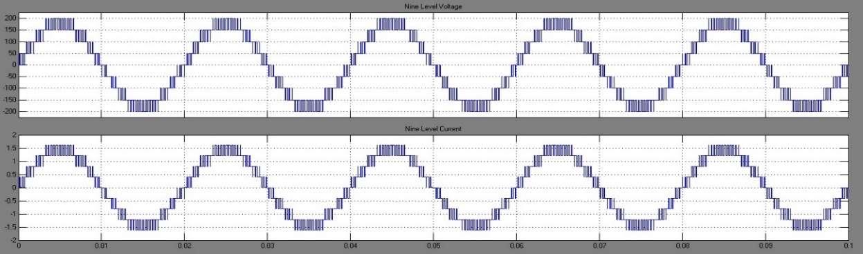
ISSN:2252-8814 Int.J.ofAdv.inAppl. Sci.Vol. 8,No.2,June2019: 143–153 150
Figure 19.Waveformsofvoltageand currentin7levelhybridMLIfor Rload
Figure20.Waveformsofvoltage andcurrentin7levelhybridinverterforRloadwithfilter
Figure21.Waveformsofvoltageandcurrentin7 levelhybridMLIforR-Lload
Figure 22.Waveformsofvoltageand currentin9levelhybridMLIfor Rload
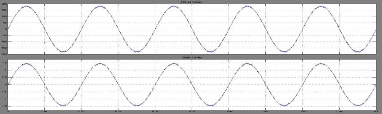
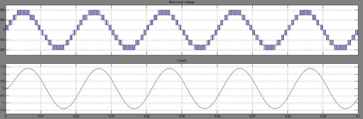
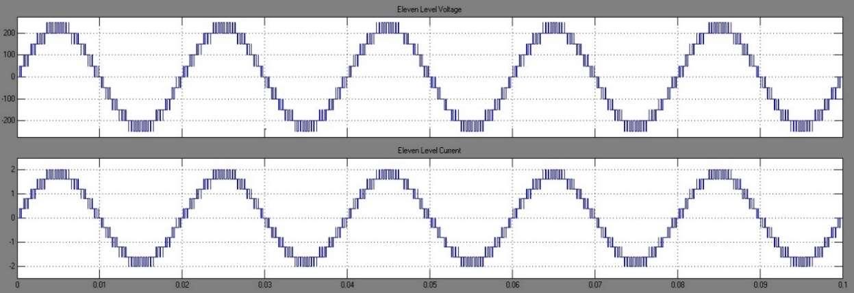
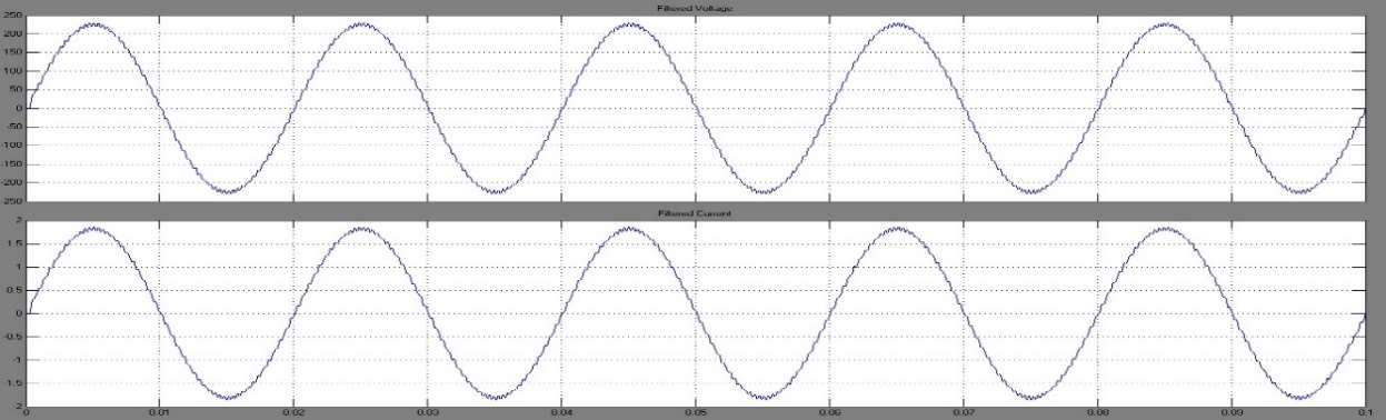
ofvoltageand currentin11levelhybrid inverterforRloadwithfilter
Perfomance evaluation and comparison of diode clamped multilevel inverter based… (N. Susheela)
Int.J.ofAdv.inAppl. Sci. ISSN:2252-8814
151
Figure23.Waveformsofvoltageandcurrentin 9levelhybrid MLIforRload withfilter
Figure24.Waveformsofvoltageandcurrentin9 levelhybridMLIforR-Lload
Figure 25.Waveformsofvoltageandcurrentin11levelhybridMLIforRload
Figure 26.Waveforms
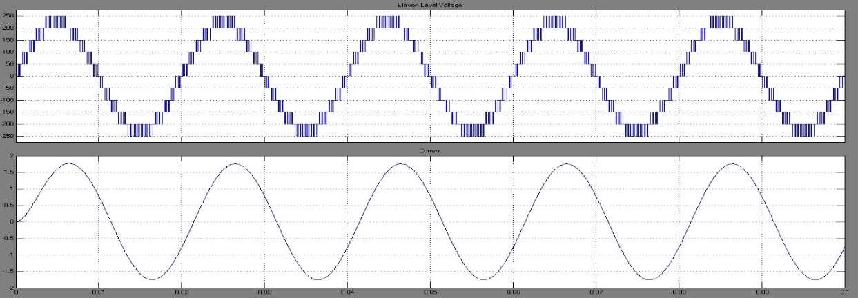
27.Waveformsofvoltageandcurrentin 11levelhybridMLIfor R-Lload
4.3. ComparisonofDCMLI andhybridMLI
Table 1 to Table 3 summarizes the comparative analysis of single phase diode clamped MLI and hybridMLIfor seven, nineand elevenlevels atvarious modulation indices (ma)usingPDand APOD SPWM techniques. It is clear that the THD decreases as the modulation index is increased. At any level, the THD of hybridinverterislesswhencomparedtoDCMLI.TheTHDisfurtherreducedusingLCfilter.
Table1.THD(%)comparisonusingPDmethodforRload
Table2.THD(%)comparisonusingAPODmethodforRLload
Table 3.CurrentTHD(%)forR-Lload
ISSN:2252-8814 Int.J.ofAdv.inAppl. Sci.Vol. 8,No.2,June2019: 143–153 152
Figure
Numberof Levels ma WithoutFilter Filter DCMLI HybridMLI DCMLI HybridMLI 7level 0.85 18.67 12.29 3.97 1.13 0.9 17.52 11.48 3.83 1.05 0.95 15.77 11.08 3.53 1 1 13.97 9.84 3.28 0.92 9level 0.85 13.19 9.05 3.55 0.88 0.9 12.81 8.47 3.42 0.87 0.95 11.97 8.4 3.18 0.85 1 10.48 7.38 3.24 0.8 11level 0.85 10.02 7.15 2.5 0.79 0.9 10.11 6.8 2.84 0.8 0.95 9.54 6.65 2.57 0.83 1 8.25 6.05 3.12 0.77
Numberof Levels ma WithoutFilter Filter DCMLI HybridMLI DCMLI HybridMLI 7level 0.85 18.5 12.21 3.18 1.1 0.9 17.58 11.56 3.01 1.02 0.95 15.74 11.12 2.93 0.99 1 13.86 9.7 2.79 0.86 9level 0.85 13.01 8.96 2.85 0.81 0.9 12.88 8.53 2.7 0.8 0.95 12.02 8.37 2.78 0.73 1 10.46 7.44 2.82 0.69 11level 0.85 9.77 7.34 2.54 0.72 0.9 10.22 6.93 2.96 0.71 0.95 9.75 6.52 2.61 0.70 1 8.38 6.02 2.84 0.66
PDmethod APODmethod 7-Level 9-Level 11-Level 7-Level 9-Level 11-Level DCMLI Hybrid inverter DCMLI Hybrid inverter DCMLI Hybrid inverter DCMLI Hybrid inverter DCMLI Hybrid inverter DCMLI Hybrid inverter 4.81 4.8 4.81 4.79 4.75 4.77 4.83 1.79 4.81 4.82 4.79 4.79 4.81 4.83 4.79 4.81 4.77 4.75 4.81 4.79 4.82 4.82 4.78 4.79 4.79 4.79 4.79 4.81 4.74 4.75 4.81 4.81 4.82 4.83 4.8 4.8 4.79 4.77 4.8 4.79 4.76 4.79 4.81 4.71 4.81 4.83 4.78 4.78
5. CONCLUSION
ThesinglephaseDCMLIandhybridMLIareimplementedforvariouslevelsatdifferentmodulation indices using PD and APOD SPWM control techniques.When compared to DCMLI, the hybrid MLI needs lesser number of high frequency switches for any number of levels. The hybrid MLI has many features compared to DCMLI in terms of the required switches, control requirements, cost, reliability and efficiency. The switches needed for various voltage levels for single phase hybrid MLI are lower compared to classical MLI’s.ThehybridMLIcanbepreferredforapplicationslike STATCOM,HVDCand FACTS.Thelowrated dc sources are required for hybrid MLI so the photovoltaic arrays and fuel cells can be utilized. The THD of DCMLI and hybrid MLI are analyzed at various modulation indices. It is observed that the THD reduces as thereisan increaseinmodulation index.Differenttypesofpulsewidthmodulation controlstrategiescanalso beusedtohybrid multilevelinverters.
REFERENCES
[1] Nabae, I. Takahashi and A. Akagi, “A new neutral-point clampedPWM inverter,” IEEE Trans. Ind. Appl., vol.19, pp.518–523,1981.
[2] G.Mondal,K.Gopakumar,P.N.Tekwani, andE.Levi,“Areducedswitch- countfive-levelinverterwith commonmode voltage elimination for an open-end winding induction motor drive”, IEEE Trans. Ind. Electron., vol. 54(4), pp.2344–2351,2007.
[3] P. M. Bhagwat and V. R. Stefanovic, “Generalized structure of a multilevel PWM inverter,” IEEE Trans. Industry Applications, vol.19(6),pp.1057-1069,1983.
[4] A. Rufer, “An aid in the teaching of multilevel inverters for high power applications,” Proc. Rec. IEEE PESC’95, pp.347–352,1995.
[5] L. M. Tolbert, F. Z. Peng, and T. G. Habetler, “Multilevel converters for large electric drives,” IEEE Trans. Ind. Appl., vol.35(1),pp.36–44, 1999.
[6] N. Susheela, P. Satish Kumar, and C. H. Reddy, “Performance Analysis of Four Level NPC and NNPC Inverters using Capacitor Voltage Balancing Method,” IEEE Uttar Pradesh Section International Conference on Electrical, Computer and Electronics Engineering,Varanasi,pp.212-217,2016.
[7] G. Carrara, S. Gardella, M. Marchesoni, R.Salutari, and G. Sciutto, “Anewmultilevel PWM method: a theoretical analysis,” IEEE Trans.Power Electronics.,vol.7(3),pp.497–505,1992.
[8] N. Susheela and P. Satish Kumar, “Performance Evaluation of Multicarrier Based Techniques for Single Phase Hybrid Multilevel Inverter using Reduced Switches,” Indonesian Journal of Electrical Engineering and Computer Science,vol.7,no.3,pp.676-686,September2017.
[9] J. Rodriguez, J.-S. Lai, and F. Z. Peng, “Multilevel inverters: A survey of topologies, controls, and applications,” IEEE Trans. Ind. Electron., vol.49(4),pp.724–738,2002.
[10] E.Najafi,A.H.M.Yatim,andA.S.Samosir,“Anewtopology-ReversingVoltage(RV)-formultilevelinverters,” IEEE 2nd International Power, Energy Conference (PECon 08),pp.604-608,2008.
[11] S. A. Gonzalez, M. I. Valla, and C. F. Christiansen, “Analysis of a cascade asymmetric topology for multilevel converters,” Proc. IEEE ISIE,pp.1027–1032,2007.
[12] N. Susheela and P. Satish Kumar, “Comparative Analysis of Carrier Based Techniques for Single phase Diode Clamped MLI and Hybrid Inverter with Reduced Components,” Indonesian Journal of Electrical Engineering and Computer Science, vol.7,no.3,pp. 687-697,September2017.
[13] E. Beser, B. Arifoglu, S. Camur, and E. K. Beser, “Design and application of a single phase multilevel inverter suitableforusingasavoltageharmonicsource”, J. Power Electron., vol.10(2),pp. 138–145,2010.
[14] G. M. Martins, J. A. Pomilio, S. Buso, and G. Spiazzi, “Three-phase low frequency commutation inverter for renewableenergy systems,” IEEE Trans. Ind. Electron., vol.53(5),pp.1522–1528,2006.
[15] Ehsan Najafi and Abdul Halim Mohamed Yatim, “Design and Implementation of a New Multilevel Inverter Topology,” IEEE Transactions on Industrial Electronics, vol.59(11),pp.4148-4154,2012.
[16] E. Babaei, “Optimal topologies for cascaded sub-multilevel converters,” J. Power Electron, vol. 10, no. 3, pp.251–261,2010.
[17] C. Govindaraju and K. Baskaran, “Analysis and implementation of multiphase multilevel hybrid single carrier sinusoidalmodulation,” J. Power Electron, vol.10(4),pp.365–373,2010.
[18] R.Stala,“Applicationofbalancingcircuitfordc-linkvoltagesbalanceinasingle-phasediode-clampedinverterwith twothree-levellegs,” IEEE Trans. Ind. Electron, vol.58(9),4185–4195,2011.
[19] N. Susheela and P. Satish Kumar, “Performance Analysis of FPGA based Diode Clamped Multilevel Inverter Fed Induction Motor Drive usingPhase Opposition Disposition Multicarrier Based Modulation Strategy,” International Journal of Power Electronics and Drive System (IJPEDS),vol.8,no.4, pp.1512-1523,December2017.
Perfomance evaluation and comparison of diode clamped multilevel inverter based… (N. Susheela)
Int.
inAppl. Sci. ISSN:
J.ofAdv.
2252-8814
153
InternationalJournalofAdvancesinAppliedSciences(IJAAS) Vol.8,No.2, June2019,pp.154~156
ISSN:2252-8814,DOI:10.11591/ijaas.v8.i2.pp154-156
Solarenergystorageandreleaseapplicationofwater-phase changematerial- (SnO2-TaC)and(SnO2–SiC) nanoparticlessystem
1FarhanLaftaRashid, 2AseelHadi, 3Ammar AliAbid, 4AhmedHashim
1DepartmentofPetroleum,CollegeofEngineering,UniversityofKerbala,Iraq
2DepartmentofCeramicsand Building Materials, CollegeofMaterials,UniversityofBabylon,Iraq
3WaterResourcesEngineeringCollege,UniversityofAl-QasimGreen,Iraq
4DepartmentofPhysics, CollegeofEducationforPureSciences, UniversityofBabylon,Iraq
ArticleInfo
Article history:
ReceivedSep15,2018
RevisedApr11,2019
Accepted May11,2019
Keywords:
Energystorage
Meltingtime
Polyethyleneglycol
Solidificationtime
Corresponding Author:
FarhanLafta Rashid, DepartmentofPetroleum, College of Engineering, UniversityofKerbala, P.O.Box1125, Kerbala,Iraq. Email:engfarhan71@gmail.com
1. INTRODUCTION
ABSTRACT
The thermal energy storage and release application of water- phase change material - (SnO2-TaC) and (SnO2–SiC) nanoparticles system has been investigated for cooling and heating applications. The water - polyethylene glycolwith (SnO2-TaC) and (SnO2–SiC) nanoparticles have been used. The resultsshowedthatthemeltingandsolidificationtimesforstorageandrelease of thermal energy of water - polyethylene glycoldecrease with increase in (SnO2-TaC) and (SnO2–SiC) nanoparticles concentrations. The melting and solidification times decrease with increasing of TaC nanoparticles concentrations to water-polyethylene glycol/SnO2 nanofluid and SiC nanoparticlesconcentrationstowater-polyethyleneglycol/SnO2nanofluid.
Copyright © 2019 Institute of Advanced Engineering and Science. All rights reserved.
Theextensivelyusedthermalenergystoragematerialsarephasechangematerials(PCMs)becauseof their ability of storing and releasing considerable amounts of energy (thermal) during the processes of phase change meltingandsolidification.Becauseofenvironmentalregardsandascentoffossilfuelscost,PCMsare attractiveincreasinglyspiritedformanyapplicationssuchas,batterythermalmanagement,electroniccooling, buildingsspaceheatingandcooling.Inthecurrentstudy,acylindricalgeometryisselectedasitisconsidered most favorable for heat exchangers, due to its acceptable efficiency in a low volume. The disadvantage of PCMs is low thermal conductivity, which decreases rates of melting and solidification [1]. Phase change materials and thermal energystoragebecomeincreasingly substantialsubjects duringthelast two decadesfor purposesof heating and cooling. When there isdelay in time between generatingenergy and energy demand, a great solution is thermal energy storage. There are three ways to store thermal energy which are sensible, latent, and chemical options. The important norm to choose a PCMs for a specific application is its phase change temperature. Also, other important parameters should also be possessed into account, including high latent heat and thermal conductivity values, in addition tocycling stability [2]. PCMs can be classified into organic and inorganic materials. The phase changes that result in absorbing heat involve conversions from solidtoliquid,liquidtovapor,andsolidtosolid.Thechangefromliquidtosolidtendstobeprioritized,given energy during the changes of transformation and minimal volumetric. PCMs should also have preferred
Journal homepage: http://iaescore.com/online/index.php/IJAAS
154
propertiessuchas:economic,thermophysical,chemical,kineticendenvironmentalfeasibilitytobeusedin passiveLHTESsystems.OthertypeofPCMscalledorganicPCMswhichcanbeclassifiedasparaffinandnonparaffinsynthesis,likealcohols,fattyacids,glycolsandesters[3].Improvedheattransfertechniquesinsolar energysystemsleadstobetterperformance.Amongmanyimprovementtechniquesinheattransfer,usingof nanofluidsasworkingfluidsinsolarcollectorsystems,waterheaters,coolingsystems,solarstilland solarcells[4].
2.MATERIALSANDMETHODS
Thewater/polyethyleneglycol(PEG)with(tinoxide(SnO2)–tantalumcarbide(TaC))and(tin oxide(SnO2)–siliconcarbide(SiC))nanoparticlessystemswerepreparedforthermalenergystorageandrelease bynanofluidswithdifferentconcentrationsofnanoparticlesarewater-polyethyleneglycol/(SnO2)0.05-x-TaCx nanoparticlesandwater-polyethyleneglycol/(SnO2)0.05-x-SiCxnanoparticles,wherex=0.005,0.01and0.015) whereSiCandTaCnanoparticleswereaddedeachonetoSnO2withconcentrationsare(10,20,and30)wt.%. The(SnO2-TaC)and(SnO2-SiC)nanoparticleswereaddedtowaterwithconcentration(1.67×10⁻³g/mL).The meltingandsolidificationprocessesduringheatingandcoolingpresentthermalenergystorageandrelease. Digitaldevicewasusedtomeasurethetemperatureduringtheheatingandcoolingprocesses.
3.RESULTSANDDISCUSSION
Theheattransferofwater/PEGwith(SnO2-TaC)and(SnO2-SiC)nanoparticlesnanofluidswas investigatedduringtheprocessesofmeltingandsolidificationasshowninFigure1toFigure4.Thetimeof meltingandsolidificationdecreaseswithincreasingof(SnO2-TaC)and(SnO2-SiC)nanoparticles concentrations.Effectivedispersionof(SnO2-TaC)and(SnO2-SiC)nanoparticlesintobasefluidwere acceleratedtheconductiveheattransferduringtheprocessofmeltingandsolidificationwherethenanoparticles formapathsnetworkinsidethenanofluids.Thewater/PEGwith(SnO2-TaC)and(SnO2-SiC)nanoparticles nanofluidscouldbeconsideredefficientforsolarwaterheatingsystemduetotheircharacteristicsofenhanced heattransfer[5-12].
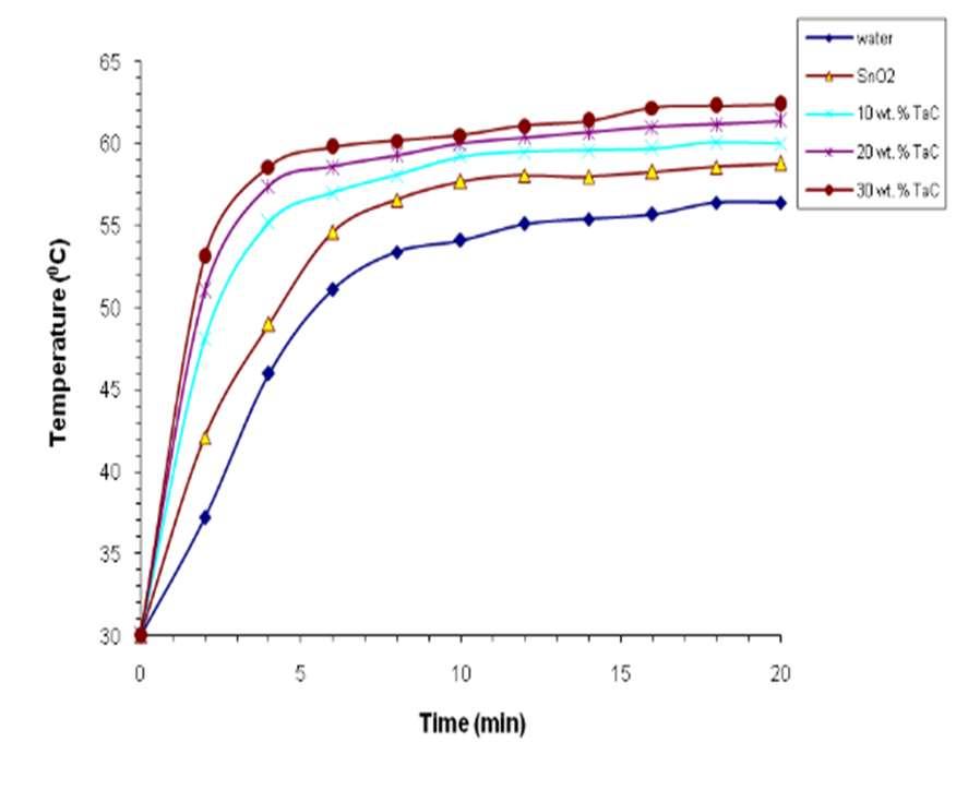
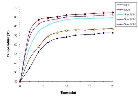
Solarenergystorageandreleaseapplicationofwater-phasechange…(FarhanLaftaRashid)
Int.J.ofAdv.inAppl.Sci. ISSN:2252-8814
155
Figure1.Meltingcurvesofwater/PEG-(SnO2-TaC) nanofluids
Figure2.Meltingcurvesofwater/PEG-(SnO2SiC) nanofluids
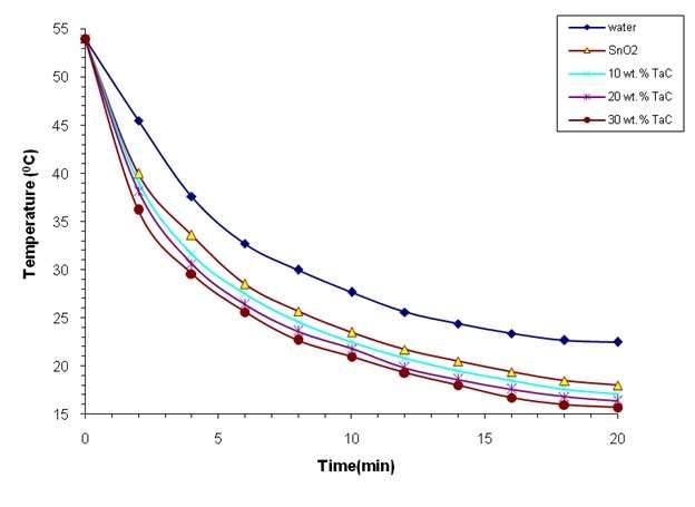
Figure3.Solidificationcurvesofwater/PEG(SnO2-TaC)nanofluids
4. CONCLUSION
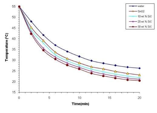
Figure4.Solidification curvesofwater/PEG(SnO2-SiC)nanofluids
The water/PEG with (SnO2-TaC) and (SnO2-SiC) nanoparticles nanofluids have high efficiency for storageandreleaseofthermalenergywhichcanbeusedforheating-coolingofbuildings,automobileengines, etc.Thetimeofmeltingandsolidificationfor storageandreleaseof thermalenergyapplicationsaredecreased withincrease ofthe(SnO2-TaC)and(SnO2-SiC) nanoparticlesconcentrations.
REFERENCES
[1] Muath A. Alomair, Yazeed A. Alomair, Hussein A. Abdullah, Shohel Mahmud, and SyedaTasnim, “Nanoparticle Enhanced Phase Change Material in Latent Heat Thermal Energy Storage System: An Experimental Study,” Proceedings of the International Conference of Energy Harvesting, Storage, and Transfer (EHST'17), Toronto, Canada,August21–23,2017.
[2] Ismaila H. Zarma, Hamdy Hassan, Shinichi Ookawara, and Mahmoud Ahmed, “Thermal Energy Storage in Phase ChangeMaterials:–Applications,AdvantagesandDisadvantages,” 1st International Cnferecne of Chemical, Energy and Environmental Engineering,HiltonAlexandiraGreen Plaza,19-21 March2017,Egypt,2017.
[3] MariaElenaArce,MiguelAnge,AlvarezFeijoo,AndresSuarezGarcia,andClaudiaC.Luhrs,“NovelFormulations ofPhaseChangeMaterials—Epoxy CompositesforThermalEnergyStoragem,” Materials,vol.11,no.195,2018.
[4] Malleboyena Mastanaiah, K. Hemachandra Reddy, and V. Krishna Reddy, “Thermal Performance Improvement of Flat Plate Solar Collector using Nano Fluids,” International Journal of Mechanical Engineering and Technology, vol.8,no.7,2017.
[5] NahedaHumood Al-Garah, Farhan LaftaRashid,AseelHadi, andAhmed Hashim, “Synthesis andCharacterization ofNovel (Organic–Inorganic)NanofluidsforAntibacterial, Antifungaland HeatTransfer Applications,” Journal of Bionanoscience,vol.12,2018.
[6] Hani Najm Obaid, Majeed Ali Habeeb, Farhan Lafta Rashid, and Ahmed Hashim, “Thermal energy storage by nanofluids,” Journal of Engineering and Applied Sciences,vol.8, no.5,pp.143-145,2013.
[7] FarhanLaftaRashid,AseelHadi,NahedaHumoodAl-Garah,andAhmedHashim,“NovelPhaseChangeMaterials, MgO Nanoparticles, and Water Based Nanofluids for Thermal Energy Storage and Biomedical Applications,” International Journal of Pharmaceutical and Phytopharmacological Research,vol.8,no.1,2018.
[8] IbrahimR.Agool,KadhimJ.Kadhim,andAhmedHashim,“Preparationof(polyvinylalcohol–polyethyleneglycol–polyvinylpyrrolidinone–titanium oxide nanoparticles) nanocomposites: electrical properties for energy storage and release,” International Journal of Plastics Technology,vol.20,no.1,pp.121–127,2016.
[9] Ahmed Hashim, Ibrahim R. Agool, and Kadhim J. Kadhim, “Novel of (Polymer Blend-Fe3O4) Magnetic Nanocomposites:PreparationandCharacterizationforThermalEnergyStorageandRelease,GammaRayShielding, AntibacterialActivityandHumiditySensorsApplications,” Journal of Materials Science: Materials in Electronics, vol.29,no.12,pp.10369–10394,2018.
[10] A.Hashimand A. Hadi, “Synthesis and characterization of novelpiezoelectricand energystoragenanocomposites: biodegradablematerials–magnesiumoxidenanoparticles,” Ukrainian Journal of Physics,vol.62,no.12,2017.
[11] Ibrahim R. Agool, Kadhim J. Kadhim, and Ahmed Hashim, “Synthesis of (PVA-PEG-PVP-ZrO2) Nanocomposites For Energy Release and Gamma Shielding Applications,” International Journal of Plastics Technology, vol. 21, no.2,2017.
[12] S. Harikrishnan and S. Kalaiselvam, “Experimental Investigation of Melting and Solidification Characterization of Nanofluid asPCM for Solar Water Heating System,” International Journal of Emerging Technology and Advanced Engineering,vol.3, specialissue:ICERTSD,pp.628-635,2013.
ISSN:2252-8814 Int.J.ofAdv.inAppl. Sci.Vol. 8,No.2,June2019:154–156 156
InternationalJournalofAdvancesinAppliedSciences(IJAAS) Vol.8,No.2, June2019,pp.157~163
ISSN:2252-8814,DOI:10.11591/ijaas.v8.i2.pp157-163
Amodelfreedissolvedoxygencontrollerforindustryeffluent usinghybridvariablesmeasuringtechnique
P.KingstonStanley1,SanjeeviGandhiA.2,D.AbrahamChandy3 1,3KarunyaInstituteofTechnologyandSciences, India 2KarpagamCollegeofEngineering,India
Article Info
Article history:
ReceivedSep19,2018
RevisedMar 25,2019
AcceptedApr15,2019
Keywords:
Dissolvedoxygen
Heteropolymer-formazin
LabVIEW
Turbidity
Waste water
ABSTRACT
The present scenario of the worldrelays on water scarcity, enormous amount of water is needed for people but the world has pollution which makes a greateffect.Wateris polluted duetovariousreasonssuchasindustrialwaste, sewage, and global warming and oil pollution and mainly polluted due to industrial effluent waste water. The main objectiveof this paper is to control thedissolvedoxygenoftheindustrialwastewaterbymeasuring turbidity and dissolved oxygen (DO). Turbidity is measured through the intensity of the light through the medium in Nephelometric unit (NTU) and dissolved oxygen is measured in PPM through amperometic electrode method. The controller isdesignedtoimprovethequalityoftheeffluentwaterthrough the aeration process. The verylowconcentration of dissolvedoxygen (DO) level is too harmful to the aquatic ecosystem and it pollutes the water to the maximum extent. This measurement method of turbidity has an enhanced idea which processed with the software and it is monitored. The controller is designed as such with the condition of inverse proportionality of water turbidity and dissolved oxygen, which contributes an additive advantage to theconceptdesign.
Copyright © 2019 Institute of Advanced Engineering and Science. All rights reserved.
Corresponding Author:
P.Kingston Stanley, KarunyaInstituteofTechnologyandSciences, KarunyaNagar,Coimbatore,TamilNadu641114,India. Email:kingstonstanley@karunya.edu
1. INTRODUCTION
The dissolved oxygen isveryimportantfactor in measuringthe water quality. The dissolved oxygen level in the water should be moderate for the aquatic life in the water. The presence of dissolved oxygen is must for the aquatic level but the range should be in some certain level. Frequently varying amount of dissolved oxygen in the water level also harm the aquatic life and pollute the water nominal rate should be processed. Lower the amount of dissolved oxygen also causes water pollution. The cloudy appearance of the water caused the presence of suspended and colloidal matter. In the waterworks field, a turbidity measurement is used to indicate the clarity of water. An improvised model predictive control is being added to already develop PI control which utilizes dissolved oxygen concentration and the air pressure of the aeration system. [1]. Control of the DO concentration in the Benchmark Simulation Model No. 1 (BSM 1) was done using the proposed T-S fuzzy neural network. A fast and efficient real time control of DO concentration in the waste treatment plant is observed by adjusting the learning rate which in turn increases the convergence rate of the system [2]. In any waste water management system oxygen is a key variable that needs to be controlled beside other variablesfor the simulation prove that the expected level of DO for MPC can be achieved [3]. An increased accuracy is possible when the weak scattered light is measured using a single photon avalanche diode (SPAD) a resolution of 0.1 NTU can be measured within 1s [4]. The Simulations results in provided segment as well as comparison results against a well-known Lyapunov based controller and a classicalPID controller [5]. The Nephelometric turbidity valuesrangesfrom 40 to 400 NTU.
Journal homepage: http://iaescore.com/online/index.php/IJAAS
157
In the activated sludge waste water treatment plant DO is a crucial factor which determines how efficiently the biological processes are taking place. Improvisation of the Direct Model Reference Adaptive control (DMRAC) is relation to DO tracking for the Sequencing Batch Reactor (SBR) is put forward [6]. The first step was to identify dissolved oxygen control loop at various operating points. By using simulation the gain scheduling controlstrategy of DO concentration was tested; an experimentally pilot plantis also presented in this paper [7]. The successful control strategies usually employ PI control for industry based applications. Effectiveness of GS-PI and MNC control methods are displayed using simulations performed on nonlinear model[8].Theprocessofsewagetreatmentisaconvolutedbiochemicalprocess. The simulationresultspoint out a better response speed, reduced overshoot and also a reduced static error is observed [9]. Waste Water treatment plant in general is a complicated, multivariable, time depended and enormous industrial system which is nonlinear. Air/Oxygen for the aerated tanks isobtained through the aeration system (blowers, pipes, diffusers). Investigation is being carried out for the nonlinear fuzzy PI control system [10]. The outcome of this study is the development of a PC based virtual (VI) system using LABVIEW, which automatically monitors and controls the Dissolved Oxygen concentration (DO). This drastically reduces business costs in terms of automation required and has higher effectiveness with lower electricity consumption [11]. The optimal set-point of dissolved oxygen affects both the batch time and energy savings. PC-based virtual instrument (VI) system using LabVIEW, which can monitor and control the dissolved oxygen (DO) concentration in an automated manner and the quality of DO is been analyzed [12]. The controllers are validated by simulation using real data sets and an ASM2d model of the biological reactor. On the consolatory aspect, three model predictive controllers (MPCs) are designed, tested and the results are compared with a PI controller.A well-established simulation benchmark isused asa test bench for this study [13]. Fuzzy logic based controlled was designed for aeration process [14]. The batch time and the energy savings are affected by the optimal set point of the parameter dissolved oxygen [15, 16]. An investigation is being carried out for the nonlinear model predictive controller and direct reference adaptive controller. Validation of the controller is done using simulated real data sets and an ASM2d model of a biological reactor [17-21]. Various model predictive controllers for dissolved oxygen in an activated sludge wastewater treatment plant (WWTP) are being discussed. This paper proposes a new system that measures turbidity and dissolved oxygen for designing an efficient DO controller. Because turbidity is inversely proportional to DO value of water. Therefore, measuring both variables and designing a controller makes the system output response better. This paper also contributes an enhanced approach of model free control for dissolvedoxygen(DO).
2. METHODOLOGY
2.1. Turbiditymeasurement
The turbidity values are measured in NTU (Nephelometric Unit). Earlier concepts measured turbidity based on the amount of light scattered through the sample medium. Instead of measuring scattered raysoflight,theothermethodissuggestedtomeasuretheintensityoflighttransmittedthroughthesample.It consists of a light source, which is a LASER emitting diode at a wavelength of 670 nm. The light from the LASER passes through the turbid solution and falls on a photo detector. The output signal from the photo detector is given asanalog input to the embedded system, where it is processed and the given analog input is calibrated Nephelometric turbidity unit and which is reported in Table 1. This turbidity measurement values are compared with standard turbidity measuring instrument. Figure 1 shows the process to measure the turbidity. Turbidity of the sample considered is inversely proportional to dissolved oxygen concentration. Thisturbiditymeasurementhelpsindesigningefficientcontroller.Differentknownsampleswerepreparedto calibrateturbiditymeter.
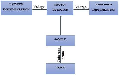
Figure 1.Turbiditymeasurementprocess
ISSN:2252-8814 Int.J.ofAdv.inAppl. Sci.Vol. 7,No.2,June2019:157–163 158
2.2.Solutionpreparation
Inordertocalibratetheturbiditymeasuringsystemthestandardformazin(heterocyclicpolymer)is preparedbythreestepprocesses[20].
Step1-PreparationofsolutionA:Dissolving1gmofHydrazinesulphatesin50mlofwateranddiluteto 100mlbyusingdistilledwater.
Step2-PreparationofsolutionB:Dissolving10gmofHexaminein50mlofdistilledwateranddiluteto 100mlindistilledwater.
Step3-FormazinPreparation:Take5mlofsolutionAanditmixwith5mlofsolutionBandallowtostand 24hoursat25ºCto30ºCtemperatureanddiluteto100mlofdistillwatertoattainastandardformazinturbid solutionof400NTU.Thestocksampleswereanalyzedandtestedtocalibratethemeasuringsystem.The chemicalreactionsareshowninFigure2.
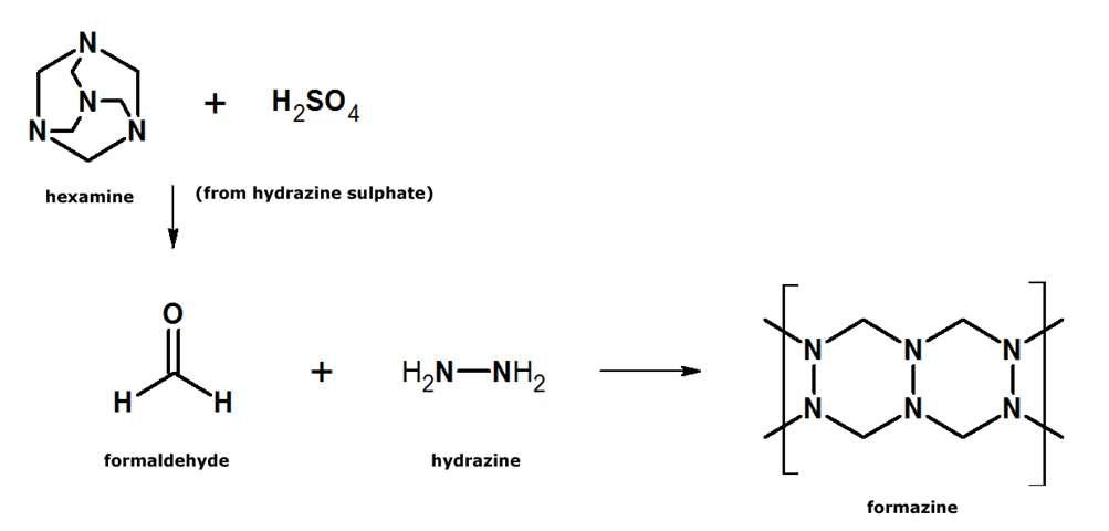
2.3.Dissolvedoxygencontrol
Basedonliteraturesurveymostoftheindustryeffluentwastewatershaveverylowdissolved oxygen.Figure3showsabouttheoverallblockdiagramofDissolvedoxygenaerationprocesscontrolin effluentwastewater.
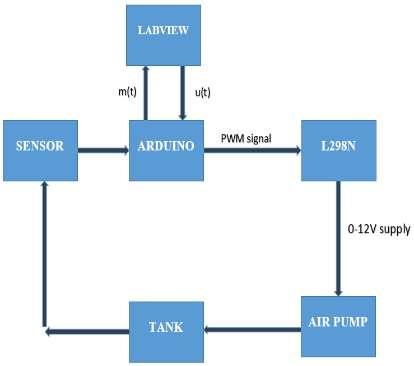
Figure3.Blockdiagramofdissolvedoxygenaerationprocesscontrol
Dissolvedoxygensensorworksbasedontheamperometricmethod.Currentflowinbetweenthe electrodesisproportionaltothedissolvedoxygenconcentrationinthewater.Analogoutputfromdissolved oxygensensorisinterfacedwithArduino.ToacquirethedatausingLabVIEW,thereisanadditional Arduinotoolinstalled.TheanalogsignalfromthedissolvedoxygensensorisgiventotheArduinoanditis directlyreadthroughLabVIEWwithoutanyspecializeddataacquisitionhardware.Theairpumpisusedas actuatordevicetoadjusttheDOlevelinthewastewaterbyvaryingtheinputvoltageofthepumprange from0-12v.
Amodelfreedissolvedoxygencontrollerforindustryeffluentusinghybrid…(P.KingstonStanley)
Int.J.ofAdv.inAppl.Sci. ISSN:2252-8814
159 Table1.Minandmaxoutputvoltagevalue SOLUTION (NTU) VOLTAGE (volts) 400.3 4004.6
Figure2.Threestepsofsolutionpreparation
Figure 4 epics the variation in the DO concentration during the aeration process by varying the pump voltage in range of 2V, 4V and 10V. By changing the pump input voltage, data’s are collected and usedfordesigninggainvaluesofPID controller.
3. RESULTSANDDISCUSSION
3.1. Experimentalresultsfor turbidity measurement
The results have obtained from the turbidity sensor using the known samples which were prepared. The analog voltage from the turbidity sensor (L14G1) is fed asvariable input through theDAQ in LabVIEW to the formula node. The formula node computes the turbidity value and which is displayed on the front panel. The resultswereshown in embedded LED display aswell as in LabVIEW. Using formula node, DAQ and While loop in LabVIEW is used to convert the LED voltage (0-5V) output to Nephelometric (40-400 NTU) Unit. Figure 5 shows the LabVIEW design for calibrating the voltage value from phototransistor into NTU. The output voltage for various values of 10 samples with different turbidity ranges are shown in Figure6.
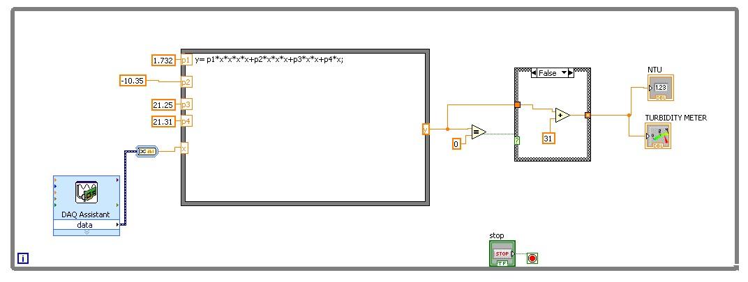
Higher order polynomial equation can improve the curve fitting relation between the input(voltage) and the output (turbidity). Therefore 4th degree linear polynomial formula which is used to convert voltage intoturbidityasfollows:
Y =q1*x^4+ q2*x^3+q3*x^2+q4*x +q5;
q1=1.732
q2=-10.35
q3=21.25
q4=21.31
q5=31
ISSN:2252-8814
160
Int.J.ofAdv.inAppl. Sci.Vol. 7,No.2,June2019:157–163
Figure4.Inputvoltagetopump
Figure 5.LabVIEWforconverting voltageto NTU
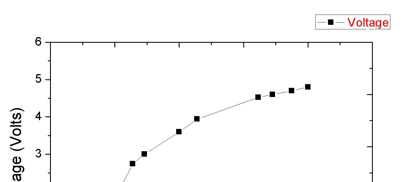
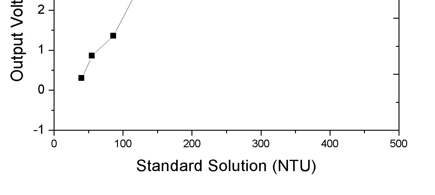
3.2. PID controllerdesignforDO
Thus the real time PID controller is implemented in LabVIEW. The set point of 5 PPM is taken to the three samples, the PID controls the process, the steady state is obtained at various load changes of each samples. The PID Controller designed using LabVIEW, is tuned using Ziegler Nicholes method and the gain ischangedby noting theresponseofthesystem.
Figure 7 shows the design of LabVIEW program to control DO level. Design of controllers are alwaysdifferent in real time implementation. ThereforePIDcontroller gain values are selected fromtrialand errormethodalsoanditssuitsforDOconcentrationsetpointtracking.Proportional&Integralcontrollersare used frequently in automation industry, especially when quickness of the response is not a matter. A control without Derivative mode is used when fast response of the system is not required and great disturbances and noise are existing during operation of the process. As the aeration process makes the DO to change quickly, Proportional,Integralandderivativegainverymuchneedforthisprocess.
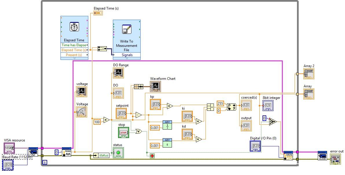
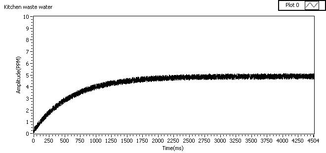
Int.J.ofAdv.inAppl. Sci. ISSN:2252-8814 A model free dissolved oxygen controller for industry effluent using hybrid … (P.
Stanley) 161
Kingston
Figure6.Samplessolutionvsoutputvoltage
Figure7.LabVIEWprogramtocontrolDOlevelusingPIDcontroller
Figure 8.PIDcontrollerresponsefordomestic wastewater
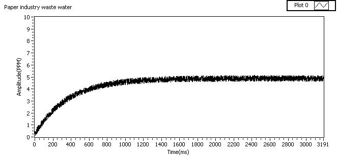
Figure9.PIDcontrollerresponseforpaperindustrywastewater
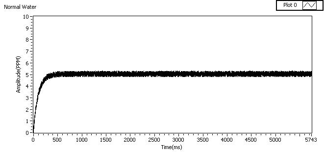
Figure10.PID controllerresponsefornormalwater
Figure 8 demonstrates the DO Control in domestic waste water. The waste water must have a minimum of 5 PPM level of DO concentration as per the literature survey. Therefore set point of 5PPM was taken to control the concentration of DO. Figure 9 indicates the DO control for paper industry waste water, the PID controller was able to achieve to the set point value of 5 PPM within 1000 milli-seconds. These experiments are tested with 30L water. The DO control for normal water is shown in Figure 10. The comparing all these three results, normal water reacts quickly to reach the set point of 5 PPM. And these experiments were performedmultiple times with fresh waters in the setup.The designed controller responses shows that the controller is able to track DO concentration effectively using hybrid variables rather than measuring single variable based DO control. Through this hybrid variables based automation process, much amountofenergycan besaved.
4. CONCLUSION
In industrial effluent and domestic waste water have measured in terms of turbidity and DO concentration. The turbidity sensor and DO sensor were calibrated with help of standard solution. The designed turbidity measurement is another method which is useful to measure colloidal particles of water in fields with a lesser conceptual cost aspect. Many phototransistors were used to improve the sensitivity of measuring turbidity values. The modelfree controller is designed to control the DO concentration effectively using both variables namely turbidity and DO concentration. The controlling of DO level concentration reduces the risk of polluting the land and can cut down many harmful factors too. The output responses of PID controllers with DO concentration level for domestic waste water; industrial effluent and drinking water were shown. From the responses it was understood the controller is effectively controlling the DO concentration without any overshoot and under shoot. The real time PID controller was successfully implemented in the pilot plant. The adaptive controller will be proposed to reduce the settling time of theprocess.
ISSN:2252-8814 Int.J.ofAdv.inAppl. Sci.Vol. 7,No.2,June2019:157–163 162
ofAdv.inAppl. Sci.
REFERENCES
[1] Gabriel Harja, Grigore Vlad, and Ioan Nascu, “MPC advanced control of dissolved oxygen in an activated sludge wastewater treatment plant,” IEEE International Conference on Automation, Quality and Testing, Robotics, 2016. [Online].Available:https://ieeexplore.ieee.org/document/7501329/.
[2] Wen-TaoFu,Jun-FeiQiao,Gai-Tang Han,and Xi Meng , “Dissolved oxygencontrolsystem basedon the T-Sfuzzy neural network,” IEEE International Conference Neural Networks, 2015. [Online]. Available: https://ieeexplore.ieee.org/document/7280506/.
[3] Xiaoxin Liu, Yuanwei Jing, Tao Ren, and Siying Zhang, “Model predictive control application in dissolved oxygen control,” IEEE Chinese Control and Decision Conference, 2015. [Online]. Avalaible: https://ieeexplore.ieee.org/document/7162095/.
[4] Huanqin Wang, Yixin Yang, Zhe Huang, and Huaqiao Gui, “Instrument for Real-Time Measurement of Low Turbidity by Using Time-Correlated Single Photon Counting Technique,” IEEE Transactions on Instrumentation and Measurement,vol.64(4),pp.1075-1083,2015.
[5] Alex Alzate, Adriana Amicarelli, Lina Gómez, and Fernando di Sciascio, “Model based predictive strategy for dissolved oxygen control applied to a batch bioprocess,” IEEE - Workshop Information Processing and Control, 2015.
[6] Piotr Hirsch, Robert Piotrowski, and Kazimierz Duzinkiewicz, “Two-step model based adaptive controller for Dissolved Oxygen control in Sequencing Wastewater Batch Reactor,” International Conference on Methods and Models in Automation and Robotics,2015.
[7] Ciprian Vlad, Sergiu Caraman, Daniela Carp, Viorel Mînzu, and Marian Barbu, “Gain Scheduling control of dissolved oxygen concentration in a wastewater treatment process,” Mediterranean Conference Control & Automatio,. 2012.
[8] C. Vlad, M. Sbarciog, M. Barbu, S. Caraman, and A. Vande, “Wouwer Indirect Control of Substrate Concentration for a Wastewater Treatment Process by Dissolved Oxygen Tracking,” Journal of control engineering and applied informatics,vol.14(1),pp.37-47,2012.
[9] Minghe Li, Jingen Peng, and Jian Wang, “Study on Smith-self-adaptive fuzzy PID controller in dissolved oxygen controlofsewagetreatment,” IEEE Conference Industrial Electronics and Applications, 2012.
[10] Zawadzki, R. Piotrowski, “Nonlinear fuzzy control of the dissolved oxygen in activated sludge processes,” IEEE Conference Emerging Technologies & Factory Automation,2012.
[11] Hsiung Cheng Lin, Liang-Tsung Huang, Lien-Fu Lai, and Yin-Fan Chi, “A remote automated system for a case studyofdissolvedoxygenmonitoring andcontrol,” IEEE International Symposium on Industrial Electronics,2009.
[12] BaiqingZhou,JuanLiu,and LuLi,“EvaluationMethodforPerformanceofReverseOsmosisAntiscalants Basedon theTurbidity,” International Conference on Electrical and Control Engineering, 2010.
[13] Jun-dong Wang, Pei-yan Li, Yong-ming Zhang, and Wei-gui Qi, “River Water Turbidity Forecasting Based on Phase Space Reconstruction and Support Vector Regression,” Intelligent Computation Technology and Automation (ICICTA), International Conference,2010.
[14] J. Ferrer, M. A. Rodrigo., A. Seco, and J.M. Penya-roja, “Energy saving in the aeration process by fuzzy logic control,” Water Science and Technology,vol.38(3),pp.209-217,2017.
[15] Ruey-Fang Yu, Cheng-Nan Chang, and Wan-Yuan Cheng, “Applying real time control to enhance the performance of nitrogen removal in the continuous flow SBR system,” Water science and Technology, vol. 38(3), pp. 271-280, 1998.
[16] Young-Hwang Kim, Chang Kyoo Yoo, and In-Beum Lee, “Optimization of biological nutrient removal in a SBR using simulation –based iterative dynamic programming,” Chemical Engineering Journal, vol. 139(1), pp. 11-19, 2008.
[17] W. Chotkowski, M. A. Brdys, and K. Konarczak, “Dissolved oxygen control for activated sludge processes,” International Journal of Systems Science,vol.36(12),pp.727-736,2005.
[18] Reza Loloee, Per A. Askeland, and Ruby N., “Ghosh Dissolved Oxygen Sensing in a Flow Stream using MolybdenumChlorideOpticalIndicators,” IEEE Sensors, 2007.
[19] Sanchez and M. R. Katebi, “Predictive control of dissolved oxygen in an activated sludge wastewater treatment plant,” European Control Conference,2003.
[20] Budi Srinivasarao, G. Sreenivasan, and Swathi Sharma, “Comparison of Dynamic Stability Response of A SMIB with PI and Fuzzy Controlled DPFC,” Indonesian Journal of Electrical Engineering and Informatics, vol. 5(3), pp.199-206,2017
[21] V. Balaji, Dr. L. Rajaji, and ShanthiniK., “Comparison Analysis of Model Predictive Controller with Classical PID Controller for pH Control Process,” Indonesian Journal of Electrical Engineering and Informatics, vol. 4(4), pp.250-255,2016.
A model free dissolved oxygen controller for industry effluent using hybrid … (P. Kingston Stanley)
Int.J.
ISSN:2252-8814
163
InternationalJournalofAdvancesinAppliedSciences(IJAAS) Vol.8,No.2, June2019,pp.164~170
ISSN:2252-8814,DOI:10.11591/ijaas.v8.i2.pp164-170
Subsynchronousresonanceoscillationsmitigationviafuzzy controllednovelbrakingresistormodel
M.Fayez1,M.Mandour2,M.El-Hadidy3,F.Bendary4
1,2,4ElectricalEngineeringDepartment,UniversityofBenha,Egypt
3EgyptianElectricityHoldingCompany(EEHC),Egypt
ArticleInfo
Article history:
ReceivedNov9,2018
RevisedApr1,2019
Accepted May2,2019
Keywords:
Chopperrectifiercontrolled brakingresistor
Fuzzylogiccontrol
Seriescompensation
Subsynchronous resonance(SSR)
Thyristorcontrolled brakingresistor
Corresponding Author: MohamedFayez, ElectricalEngineering Department, UniversityofBenha, Shoubra,Cairo108,Egypt. Email:eng_mf69@yahoo.com
ABSTRACT
Subsynchronousresonance(SSR)torsionaltorqueoscillationsisaproblemof a great concern in the power engineering community. SSR causes torsional torque oscillations with ever-increasing magnitudesoccurring in the machine shaft sections causing a premature fatigue life expenditure of the shaft metal. Inthispaper,dynamicbrakingswitchingstrategydesignedthroughfuzzylogic control theory and implemented via novel braking resistor model, namely chopper rectifier controlled braking resistor for tempering SSR torsional torqueoscillationsofalargeturbo-generator.Theproposedmitigationscheme has been tested on the IEEE second benchmark model for SSR studies. Comparative simulation study via MATLAB/Simulink-based modeling and simulation environment of the test model with and without the suggested mitigation regime should demonstrate its effectuality for mitigation of SSR torsionaltorqueoscillations.
Copyright © 2019 Institute of Advanced Engineering and Science. All rights reserved.
1. INTRODUCTION
Usually,therotorofasteamturbine-generatorsetisconsideredasasinglerotationalmasswithcertain inertia constant in the analysis and investigation of many power system dynamic problems[1]. But, the rotor of a steam turbine-generator is a highly complicated mechanical structure. The rotor of a steam turbinegenerator set (i.e. shaft train) is composed of a string of dominant massive elements, each one has a considerable inertia constant and relatively large diameter, rigidly connected in tandem at the thinner shaft extensions[1].The completeshafttrain cansurpass50metersoftotallengthandweightseveralhundredtons [1]. The spring-mass model of the turbine-generator shaft is prerequisite for elucidating the torsional torque oscillations occurring at the shaft extensions [1]. SSR torsional torque oscillations is a problem of a great concern in the power engineering community [1, 2]. SSR is a transmission system-based problem that causes adversedevastatingeffectsontheturbine-generatorsetsoperatingunderthiscircumstance[2].Therefore,SSR isconsideredasmultidisciplinarypowerutilityproblem.
In 1970, and again in 1971, a 909 MVA cross-compound turbine-generator at Mohave coal-fired powerplantinsouthernNevada,California,USA,hadencounteredcollectorringdamageinthehigh-pressure unit exciter shaft due to SSR torsional torque oscillations [2, 3]. The devastating consequences of Mohave accidents have fed off the industry’s enthusiasm about this phenomenon to find reliable mitigation countermeasures and underscored the urge for quickly implementing them [3]. SSR causes torsional torque oscillations with ever-increasing magnitudes occurring in the machine shaft sections causing a premature fatiguelifeexpenditureoftheshaftmetal[1-5].The shaftisthendefinitelydestinedtoexperienceirrevocable
Journal homepage: http://iaescore.com/online/index.php/IJAAS
164
low-cycle fatigue cracks or even a complete shaft fracture [1-5]. SSR arises in power plants, especially with steam-turbineprimemovers,asanundesirablecollateralresultfortransmissionlinesemanatingfromapower plant and equipped with series capacitors at certain conditions [1-5]. The fatigue damage of large turbinegeneratorshaftisdefinitelyundesirableandcatastrophiceventinthepowerindustry[5,6].Thisisbecausethe shaft rehabilitation process is very expensive and takes several months to be accomplished during which the unit is intuitively out of service [6]. Also, during the shutdown shaft rehabilitation period, the plant should purchase the electric energy required to energize the auxiliary equipments of the plant from the utility which brings more economic casualties to the plant owner beside the inability to sell the output electrical energy of theplant[6].
Seriescompensationhasbeenwidely utilizedby theutility since 1952foreconomicallytransmitting bulk power transactions over long transmission distances [7]. Series compensation has many overwhelming benefits. It aggrandizes the electric power transferring capability of long transmission corridor, enhances the voltage profile of the grid, and boosts the angular stability of the system and so forth [7]. At certain cases, series compensated power systems are vulnerable to have SSR condition in which the series compensated electric system interchanges a considerable amount of energy with a turbine-generator mechanical system at one more of the natural frequencies of the combined electromechanical system below the synchronous frequencyoftheelectricsystem[4-6].
For the sake of secure operation of bulk power systems, large turbo-generators are certainly needed to be in service for as long as possible due to their active and reactive power supplying capabilities [5]. So, utilizing protection relays to protect large units from SSR conditions will not generally be considered except as a final sanctuary [5]. Therefore, SSR mitigation countermeasures should alleviate the devastating SSR torqueoscillationsandeliminatetheneedtotriptheunitsthatarepronetoresonantcondition.Therehavebeen a considerable number of technical studies and research papers addressing the SSR problem and presenting many mitigation countermeasureswithcontrol algorithms, mitigation equipmentsizes, and the mosteffective locationinthenetworkfortheseprospectivemitigationcandidates[6].
SeveralmitigationapproacheshavebeendevelopedfortemperingofSSRoscillationssuchas,Static VAR Compensator (SVC), Thyristor-Controlled Series Capacitor (TCSC), Static Synchronous Series Compensator (SSSC), Static Compensator (STATCOM), Unified Power Flow Controller (UPFC), and excitationsystemcontrolthroughusinganappropriate supplementarystabilizingsignal[8-10].
Among the multiple presently conceivable SSR mitigation candidates, the dynamic braking resistor (BR) is an extremely effective and relatively cheap mitigation candidate for SSR problems [10-15]. BR was initiallyimplementedforaugmentingtransientstabilityofelectricpowersystems[1].BRfunctionsasapseudo electric load withtheability to consume themomentarilyaccelerating energyinpowersystemsarising dueto severe nearby faults, especially in power systems with hydro dominated power plants [1]. Therefore, by dissipating the extra generated power, BR should prohibit generator pole slipping conditions and thereby augmenting the transient stability of electric power systems [1]. Bonneville Power Administration (BPA) dynamicbrakeisoneofthelargestexistingBRinstallationsinrealisticpowersystemswithpowerdissipation ability of 1400 MW with230kVrated voltage [1]. Many worksofliterature have addressed the utilizationof BR connected to the grid via a three-phase AC voltage controller, i.e. thyristor controlled braking resistor (TCBR), for mitigation of multi-modal shaft torsional oscillations [15-20]. TCBR per phase model is constructed as two back-to-back connected high-power thyristor valves with BR in series which means that threeBRswereutilizedforSSRtorsionaloscillationsmitigation[16-20].
Very recently, a novel BR model, namely Chopper Rectifier Controlled Braking Resistor (CRCBR) model, is introduced to the academic community as an alternative innovative mean for implementing the concept of dynamic braking interventions for enhancing the transient stability of power systems [21-23]. In [21,22],theeffectivenessofCRCBRfortransientstabilityenhancementinsinglemachineinfinitebus(SMIB) system and the Western System Coordinated Council (WSCC), 3-machine 9-bus system, respectively, have beentested.CRCBRcontrolledthroughafuzzylogiccontroller(FLC)isproposedinthisarticleformitigation of SSR torsional oscillations. CRCBR is fundamentally a single BR bank linked to the three-phase terminals of the synchronous generatorthrough a three-phasefull-wave uncontrolled rectifierdiodebridge and chopper switch(CS) [21,22].
No similar work could be found in the literature to date regarding the utilization of CRCBR for mitigation ofSSRtorsionaltorqueoscillations. The CRCBRiseitherswitchedONorswitchedOFFbasedon theenergizationsignalproducedbytheFLC.Thegeneratormassspeeddeviationisimplementedinthiswork asalocalcontrolinputsignaltotheFLCforstrategizingtheCRCBRswitchingintervals.Theinfluenceofthe proposed scheme in mitigating SSR torsional oscillations is tested in this work using the IEEE second benchmark model via MATLAB/Simulink-based modeling and simulation environment. Comparative simulation study of the test system with and without the suggested mitigation regime should demonstrate its effectualityformitigationofSSRtorsionaltorqueoscillations.
Int.J.ofAdv.inAppl. Sci. ISSN:2252-8814 Subsynchronous resonance oscillations mitigation via fuzzy controlled novel braking … (M.
165
Fayez)
The rest of this paper is organized as follows. In section 2, the well-known test system is briefly described. In section3the concept ofutilizing the FLC toorchestrate the switching strategy oftheCRCBRis introduced.Insection4,MATLAB/Simulinktimedomainsimulationresultsaredelineatedwithcomments.In section5,thekeyconclusionsofthisworkare drawn.Finally,the referencesusedinthisworkarelisted.
2. SYSTEMMODEL
Toscrutinizetheeffectivenessofthesuggestedmitigationregimeinthispaper,thewell-knownIEEE secondbenchmarkmodelforcomputersimulationofSSRisadopted.Figure1depictsthesinglelinediagram ofthesystemunderstudytogetherwithCRCBRandthesteamturbine-generatorshaftdetail[21-23].TheIEEE second benchmark model is basically a single synchronous generator (600 MVA/22kV/60 Hz/3600 rpm) connected to an infinite bus through generator step-up transformer (600 MVA/22kV/500kV) and two extrahigh voltage (EHV) transmission lines, one of which is equipped with a series capacitor of 55% seriescompensation ratio. The generator is driven by one single-flow high-pressure (HP) steam turbine and one double-flow low-pressure (LP) steam turbine connected intandem.ThemodelofCRCBR consistsofoneBR bankconnectedtothegeneratorterminalsviasix-pulsefullwaveuncontrolledRectifierBridgeandachopper switchasshowninFigure1[21-23].Inthisarticle,theInsulatedGateBipolarTransistor(IGBT)isutilizedas achopperswitch.TheBRbankisassumedtobecapableofdissipating50%theconnectedgeneratorapparent power(i.e.300MW).
Figure 1.The IEEEsecondbenchmarkmodelwithaturbinegeneratorshaftmulti-mass modelincorporatingchopperrectifiercontrolledbrakingresistordevice [21-23]
The brake is switched ON or OFF via the chopper switch to mitigate the shaft torsional oscillations by reducing the net available energy for acceleration and hence speed deviation of the generator mass due to severe disturbances such as system close in faults [1]. The proposed scheme utilizes a local control signal represented by the generatormass speed deviation to help the FLC determine whether the CRCBR should be switched ON or switched OFF. The system is completely modeled in MATLAB/Simulink environment. The electrical parameters for the synchronous generator are obtained from [23]. The under-study steam turbine configuration is appropriately illustrated in [23]. It consists of HP section and single LP section. The turbine contributing torque fractions for the turbine sections HP, and LP are 50%, and 50%, respectively [23]. The detailedturbine-generatorshaftmechanicaldataisobtainedfrom[23].Theelectricalparametersofthesystem inper-unit,with100MVAasacommon basepower,arealsoobtainedfrom[23].
3. FUZZYLOGICCONTRLLERDESIGN
The fuzzy logic is differing from the crisp logic in Boolean theory which utilizes only two logical levels(0 or 1) in thatitusesunbounded logicallevels(from0 to 1) to dealwith issues thathaveuncertainties orobscuresituations[24-26].FLCsaredemonstratedtobemorerobustandtheirperformancespossessalesser sensitivity to the parametric differencesthan the traditional controllers [24-26]. Recently, fuzzy-logic control has gained a reputation in effectively solving many power system dynamic problems [24-26]. FLC is a nonlinear controller with a rule-based system,in other words, itisan artificial-intelligence (AI) based system
ISSN:2252-8814 Int.J.ofAdv.inAppl. Sci.Vol. 8,No.2,June2019: 164–170 166
G LineA 600MVA-60Hz 22kV-500kV F1 Δω_G LineB FiringCircuit A B C FLC Gatesignal B500 B500 B22 LPHP TLP-GenTHP-LP G 600MVA22kV 3600rpm 300 MW Rectifier Bridge InfiniteBus Cs=55% Turbine-Generator Set Generator Terminals A B C BR Chopper Switch Chopper Switch
whichreliedontheuseofexpertknowledge[24-26].Thisexpertknowledgeiscommonlyacquiredthrough conductingcomprehensivemathematicalmodeling,analysis,anddevelopmentofcontrolalgorithmsforthe powersystems[24-26].Asetoffuzzylinguisticrules,usuallydistinguishedby“IF-THEN”statements, representingacontroldecision-makingmechanismresponsibleforregularizingtheeffectuationsforsystem stimulants[24-26].ThebasicFLCconfigurationconsistsofthefollowingfourprimestages:fuzzification, knowledgebase,inferenceengine,anddefuzzification[24-26].Inthefuzzificationstage,thecrispinputvalues aremappedintofuzzyvariablesbyusingnormalizedmembershipfunctionsandoccasionallyinputweighting factors[24-26].Thefuzzy-logicinferenceengineappropriatelydeducesthesuitablecontrolactionbasedon theattainablerulebase[24].TwomajorinferenceenginetypesareTakagi-Sugeno(TS),andMamdani[27]. Thefuzzycontrolactionisconvertedtopropercrispvaluethroughthedefuzzificationprocessusing normalizedmembershipfunctionsandoccasionallyoutputweightingfactors[24-26].
TStypeismoreefficientthantheMamdanitypefordynamicsystemswithfastchangingdynamics becauseitworkswellwithlinear,adaptiveandoptimizationtechniquesanditiswellsuitedtomathematical analysis[27].Therefore,TSinferencemechanismisutilizedinthesimulationstudy.Theoverlappingofthe membershipfunctionsmakesthemappingsmootherandenhancesthecontrollerperformance[24].
Ithasproventhatthedampinglevelobtainedfromusingthegeneratormassspeeddeviationasthe controllerinputisbetterthanthedampinglevelobtainedfromusingotherturbinesectionsspeeddeviation signals[17,20].Also,thegeneratormassspeedsignalisnotsodifficulttocapturelikeHP,andLPspeed signalssincetheentiresteamturbineisrigorouslysealedwiththeoutercasesviasteamsealsystem.So,the generatormassspeeddeviationinper-unit,Δɷ,isselectedasinputtotheFLCwhiletheoutputsignalis constantwitheither0or1.TheoutputsignalofFLCisthensenttotheIGBTgatingcircuitwhichproducesthe gatesignalsforthechopperswitchbasedonthecontrollerdecisionoutput.
TheGaussianandSigmoidinputsmembershipfunctionsareshowninFigure2inwhichthree linguisticvariables,NB(NegativeBig),Zo(Zero)andPB(PositiveBig),aredefiningthefuzzinessofthe controllerinput.Themembershipfunctionsparametersaredeterminedbytrialanderroraccordingtothe generatormassspeeddeviationswingrangebasedonanextensivesimulationstudy.Theoutputtypeisconstant havingeither0or1values(0forbothZOandNB,1forPO).Where0indicatesthattheIGBTshouldbein OFFstateand1indicatesthattheIGBTshouldbeinONstate.
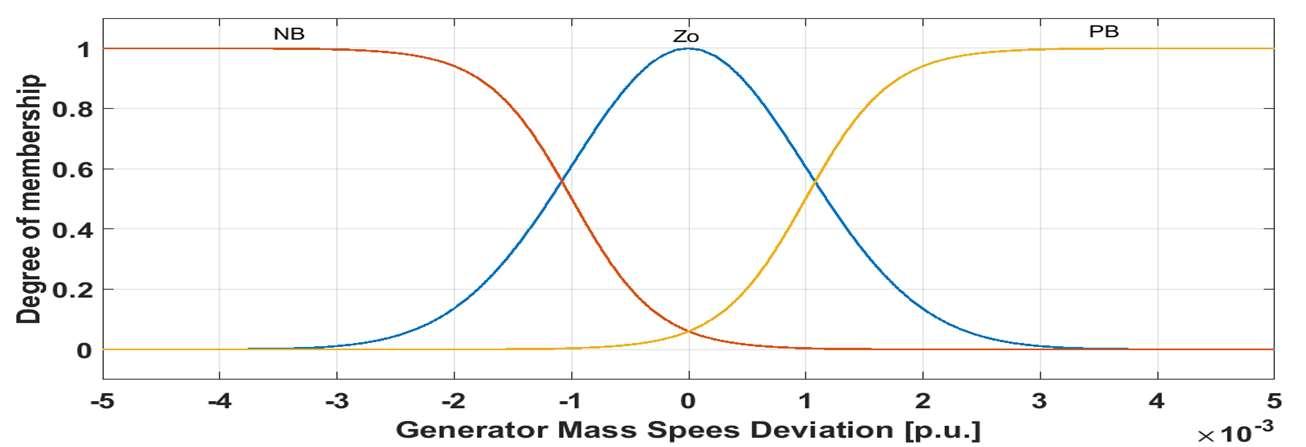
Theproposedcontrolschemeisverystraightforwardandsimplesinceithasonlythreecontrolrules wheretheBRisinsertedifthegeneratorspeeddeviationexceedsacertainvalue(theaccelerationstate)and removedelsewhere(steadystateanddecelerationstate).Therearethreepremisemembershipfunctions depictedinFigure2,oneforeachrule,andtheconclusionsaresingletonsothefuzzycontrolrulesareas follows,Iftheinput(Δɷ)isNBthentheoutputis0,Iftheinput(Δɷ)isZothentheoutputis0andIftheinput (Δɷ)isPBthentheoutputis1.
4.SIMULATIONRESULTS
Tofurtherdemonstratetheeffectivenessoftheproposedmitigationregime,timedomainsimulation studyviaSimulinkmodeliscarriedout.Three-phasetoground(3LG)self-healingfaultisappliedatlineB, veryclosetogeneratorhighvoltagebusatfaultpointF1,asshowninFigure1.Thefaultisappliedat0.25 secondfromthesimulationtimeof5seconds.Thefaultisself-clearedafter0.0169secondsfromtheinception ofthedisturbance.Thetorsionaltorqueprofilesofturbine-generatorshaftsysteminper-unit(p.u.)andthe speedresponsesofturbine-generatordifferentmasseswithandwithoutthefuzzy-controlledCRCBRarelisted asafamilyofcurvesshowninFigure3andFigure4.
Subsynchronousresonanceoscillationsmitigationviafuzzycontrollednovelbraking…(M.Fayez)
Int.J.ofAdv.inAppl.Sci. ISSN:2252-8814
167
Figure2.FLCinputmembershipfunctionsinper-unit
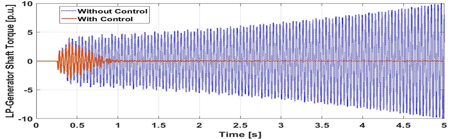
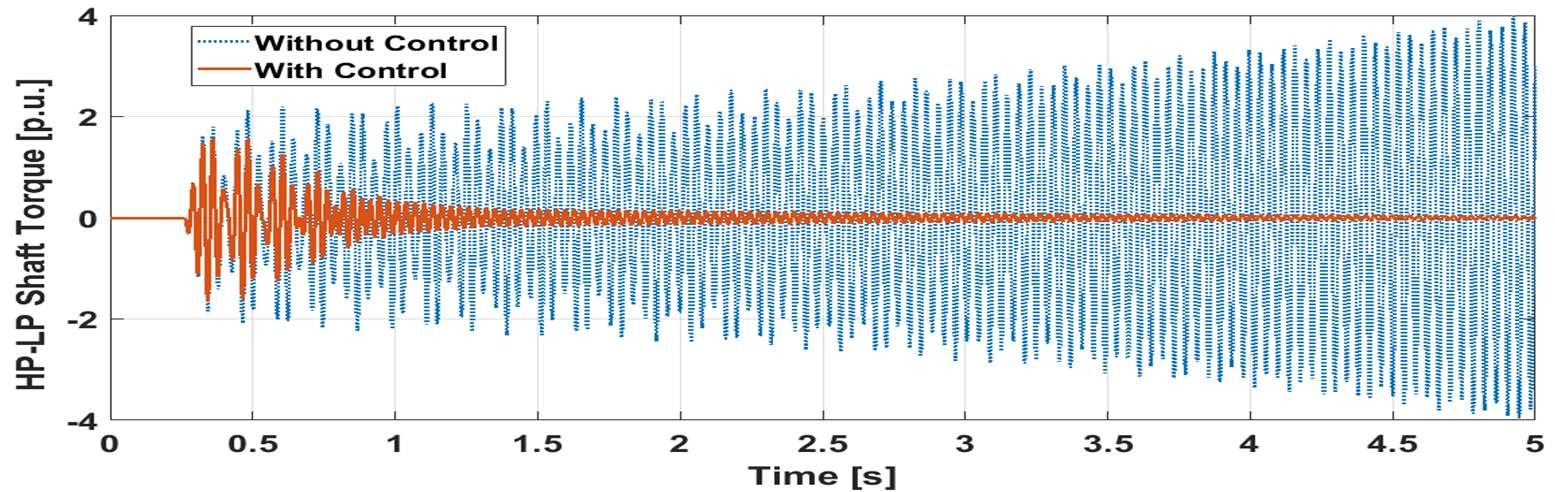
Figure3.TorqueresponseswithandwithoutfuzzycontrolledCRCBR duetothethree-phaseself-healingfaultatthegeneratorHVbusinp.u., (a)LPturbine-generatorshafttorsionaltorque,(b)HP-LPShafttorsionaltorque
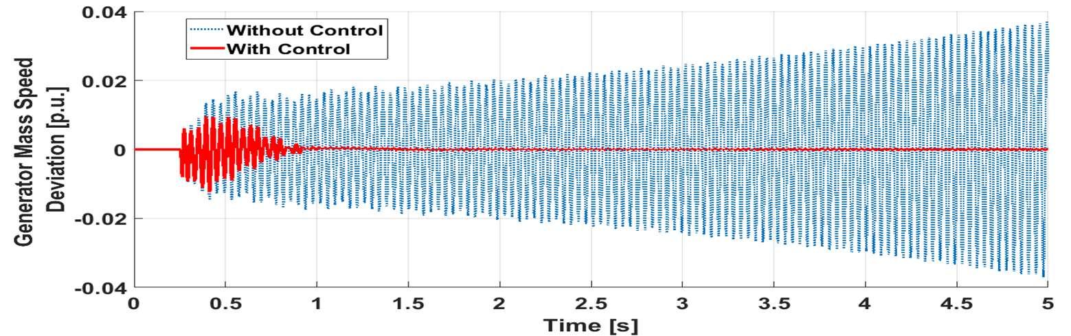
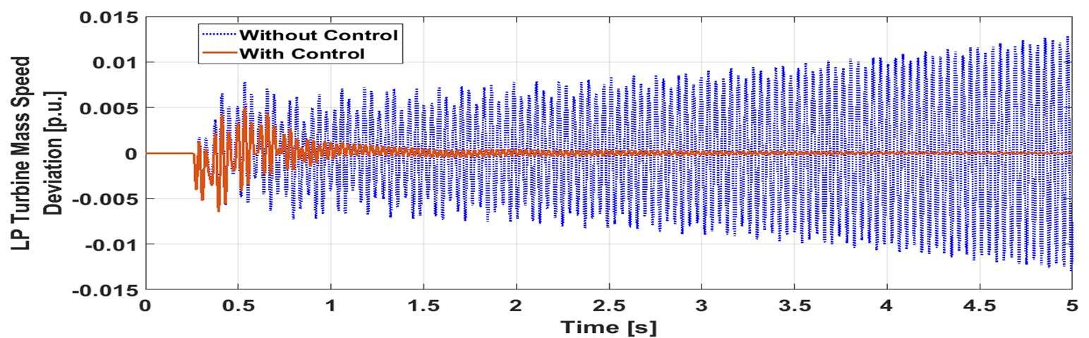
Int.J.ofAdv.inAppl.Sci.Vol.8,No.2,June2019:164–170
ISSN:2252-8814
168
(a)
(b)
(a)
(b)
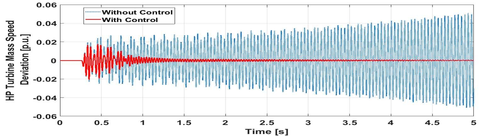
Figure4.Relativeturbine-generatormassspeedresponsesduetothethree-phaseself-healingfaultatthe generatorHVbusinp.u.,(a)Generatormassspeeddeviation,(b)LPturbinemassspeeddeviation, (c)HPturbinemassspeeddeviation.
Finally,inFigure5itisshownthecomparativeresponsesofthemechanicalrotorangledeviationfor thesynchronousgeneratorunderthegivenfaultcondition.Duetoapplyingtheproposedtechniquethe oscillationsintherotorangleissettledafter1secondfromtheperturbationinitiation.
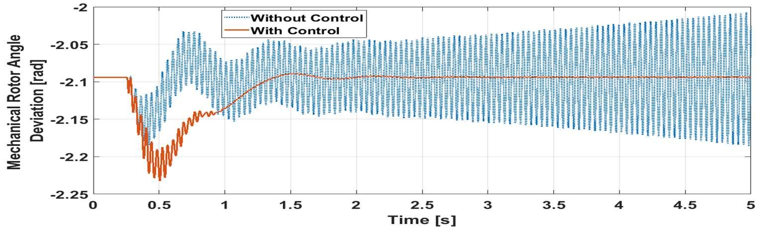
AsevidencedfromthesimulationresultsportrayedinFigure3,Figure4andFigure5,inthebase casesimulationresultswithouttheproposedscheme,itisclearlyseenthatbothspeedandtorqueresponses seemtobesustainedwithever-increasingamplitudesinthetimeframeofthesimulationwhichindicatesthe unstablenatureoftheresponses.Thedrivingmechanicaltorquetransmittedbetweentheshaft'smasseshave experienceddevastatingoscillationswithextremelyunacceptableamplitudes.Thesetorqueoscillationswill, forsure,endupcausingaprematureshaftfatiguelifeexpenditureandirrevocableshaftcracksorevenashaft fracturewiththeunpleasantoutcomes.DuetoapplyingthefuzzycontrolledCRCBR,itisobviouslyshown thattheshafttorsionaloscillationsofaturbine-generatorsetandthespeedresponseshaveexperiencedan excellentsupplementarydamping,whichfurtherenablestheutilizingofseriescompensationsafelynearthe steampowerplantswithoutanymechanicaljeopardy.
5.CONCLUSION
ThispaperauthenticatestheeffectivenessofCRCBRcontrolledviaFLCtodampSSRshafttorsional oscillations.Fromthesimulationresults,thespeedandthetorqueprofilesofthemachinemanifesta significantlygoodsupplementarydampingwhichallowsthetorsionaloscillationsandthespeedoscillationsto dieoutquickly.UtilizingonlyoneBRunit,insteadofthreeunitsincaseofTCBR,mightencouragetheutilities touseitfordampingtheshafttorsionaloscillationsarisingfromSSRconditionsandcompromisebetweenthe benefitsofimplementingseriescompensationandtheconcernsofthemachineshaftdamage.TheCRCBRis consideredasaviablemeanforboostingthesecurityofthepowersystemfromtheoperationalperspectiveby extendingthefatiguelifeoftheunitsinthepowersystemtotheirmaximumpossiblepotentialbyneutralizing anySSRcondition.Finally,implementingtheproposedschemeshouldcapacitateconventionalseries compensationontransmissionlinesemanatingfromthermalpowerplantssafelyandsoundlywithout jeopardizingtheshaftmechanicalintegrityoftheturbine-generatorset.
Subsynchronousresonanceoscillationsmitigationviafuzzycontrollednovelbraking…(M.Fayez)
Int.J.ofAdv.inAppl.Sci. ISSN:2252-8814
169 (c)
Figure5.Mechanicalrotorangledeviationin[rad]
REFERENCES
[1] M. Fayez Ahmed, et al., “Torsional Oscillations Mitigation for Interconnected Power System via Novel Fuzzy Control Based Braking Resistor Model,” Conseil International des Grands Réseaux Électriques (CIGRÉ), Paris, France,August26-31,pp.1–9,2018.
[2] EPRI Technical Report 1011679, “Steam Turbine-Generator Torsional Vibration Interaction with The Electrical Network,”ElectricPowerResearchInstitute(EPRI),2005.
[3] Geoff Klempner and Isidor Kerszenbaum, Handbook of Large Turbo-Generator Operation and Maintenance. John Wiley &Sons,2008.
[4] DuncanN.Walker, Torsional Vibration of Turbomachinery.McGraw-Hill,2003.
[5] P. M.Anderson, Power system protection.JohnWiley&Sons,1999.
[6] LeonardL.Grigsby, Power system stability and control,Third edition.CRCPress,2012.
[7] Mircea Eremia, Chen-Ching Liu, and Abdel-Aty Edris, Advanced solutions in power systems HVDC, FACTS and artificial intelligence.JohnWiley&Sons,2016.
[8] R.MohanMathurandRajivK.Varma, Thyristor-based FACTS controllers for electrical transmission systems.John Wiley &Sons,2002.
[9] Shruthi Ramachandra, et al., ”Dynamic bifurcation analysis and mitigation of SSR in SMIB system,” Indonesian Journal of Electrical Engineering and Computer Science, vol.15,no.3, 2019.
[10] S. Helmy, et al., “Mitigating subsynchronous resonance torques using dynamic braking resistor,” International Middle East Power Systems Conference (MEPCON), Egypt,2010,pp.416–421.
[11] Li Wang, and Ching-Huei Lee, “Application of dynamic resistance braking on stabilizing torsionaloscillations,” in International Conference on Computers, Communications and Automation,Beijing,China,1993,pp.145–148.
[12] R. M. Hamouda, et al., “Damping Torsional Oscillations in Large Turbo-Generators Using Thyristor Controlled Braking Resistors,” in 2008 Australasian Universities Power Engineering Conference (AUPEC'08), Australasia, 2008,pp.1–6.
[13] A.H.RahimandH.M.Al-Maghraby,“DynamicBrakingResistorforControlofSubsynchronousResonantModes,” IEEE Power Engineering Society Summer Meeting, Seattle,WA,USA,2000,pp.1930–1935.
[14] A. H. M. A. Rahim and H. M. AI-Maghraby, “Control of SSR Oscillations Through A Quasi-Optimum Dynamic BrakingStrategy,” International Journal of Power and Energy,vol.23,pp.90–95,2003.
[15] A.H.M.A.Rahim,“AMinimum-TimeBasedFuzzyLogicDynamicBrakingResistorControlforSub-Synchronous Resonance,” Electrical Power and Energy Systems,vol.26,pp.191–198,2004.
[16] O. Wasynczuk, “Damping Shaft Torsional Oscillations Using A Dynamically Controlled Resistor Bank,” IEEE Transactions on Power Apparatus and Systems,vol.100,pp.3340–3349,1981.
[17] EPRITechnicalReport103902,“DynamicBrakeControltoReduceTurbineShaftTransientTorque,”ElectricPower ResearchInstitute(EPRI),1994.
[18] M. H. Ali, et al., “Minimization of Shaft Torsional Oscillations by Fuzzy Controlled Braking Resistor Considering Communication Delay,” WSEAS Transactions on Power Systems,vol.3,pp.174–179,2008.
[19] M. H. Ali, et al., “Coordination of Fuzzy Controlled Braking Resistor and Optimal Reclosing for Damping ShaftTorsionalOscillationsofSynchronousGenerator,”in International Conference on Electrical Machines and Systems (ICEMS), Seoul,SouthKorea,2007,pp.1259–1264.
[20] M. H. Ali, et al., “A fuzzy Logic Controlled Braking Resistor Scheme for Damping Shaft Torsional Oscillations,” IEEJ Transactions on Power and Energy,vol.124,pp.207–214,2004.
[21] R. Saluja and M. H. Ali, “Novel Braking Resistor Models for Transient Stability Enhancement in Power Grid System,” IEEE PES Innovative Smart Grid Technologies (ISGT) Conference,WashingtonDC,USA,2013,pp.1–6.
[22] R. Saluja, S. Ghosh, and M. H. Ali, “Transient stability enhancement of multi-machine power system by novel braking resistormodels,” Proceedings of the IEEE Southeast Conference,Florida,USA,2013,pp.1– 6.
[23] IEEE Committee Report, “Second Benchmark Model for Computer Simulation of Subsynchronous Resonance,” IEEE Transactions on Power Apparatus and Systems,vol.l04,pp.1057–1066,1985.
[24] M.FayezAhmed, et al.,“TorsionalOscillationsMitigationviaNovelFuzzyControlBasedBrakingResistorModel,” International Electrical Engineering Journal (IEEJ),vol.7,pp.2173–2181,2016.
[25] Gilfred Allen Madrigal, et al., “Fuzzy logic-based maximum power point tracking solar battery charge controller with backup stand-by ACgenerator,” Indonesian Journal of Electrical Engineering and Computer Science, vol.16, no.1,pp.136-146,2019.
[26] Salam Waley Jeaeb, et al., “Advanced optimal by PSO-PI for DC motor,” Indonesian Journal of Electrical Engineering and Computer Science, vol.16,no,1,pp.165-175,2019.
[27] S. Mohagheghi, et al., “Modified Takagi-Sugeno Fuzzy Logic-Based Controllers for A Static Compensator in A Multi-MachinePower System,”in Industry Applications Conference,Seattle,USA,2004,pp.2637–2642.
ISSN:
Int.J.ofAdv.inAppl. Sci.Vol. 8,No.2,June2019: 164–170 170
2252-8814
Institute of Advanced Engineering and Science
Indonesia : D2, Griya Ngoto Asri, Bangunharjo, Sewon, Yogyakarta 55187, Indonesia
Malaysia : 51 Jalan TU 17, Taman Tasik Utama, 75450 Malacca, Malaysia
COPYRIGHT TRANSFER FORM
(Please compile this form, sign and send by e-mail)
Please complete and sign this form and send it back to us with the final version of your manuscript. It is required to obtain a written confirmation from authors in order to acquire copyrights for papers published in the International Journal of Advances in Applied Sciences (IJAAS)
Full Name and Title
Organisation
Address and postal code City Country Telephone/Fax
Paper Title
Authors
Copyright Transfer Statement
The copyright to this article is transferred to Institute of Advanced Engineering and Science (IAES) if and when the article is accepted for publication. The undersigned hereby transfers any and all rights in and to the paper including without limitation all copyrights to IAES. The undersigned hereby represents and warrants that the paper is original and that he/she is the author of the paper, except for material that is clearly identified as to its original source, with permission notices from the copyright owners where required. The undersigned represents that he/she has the power and authority to make and execute this assignment.
We declare that:
1. This paper has not been published in the same form elsewhere.
2. It will not be submitted anywhere else for publication prior to acceptance/rejection by this Journal.
3. A copyright permission is obtained for materials published elsewhere and which require this permission for reproduction.
Furthermore, I/We hereby transfer the unlimited rights of publication of the above mentioned paper in whole to IAES The copyright transfer covers the exclusive right to reproduce and distribute the article, including reprints, translations, photographic reproductions, microform, electronic form (offline, online) or any other reproductions of similar nature.
The corresponding author signs for and accepts responsibility for releasing this material on behalf of any and all co-authors. This agreement is to be signed by at least one of the authors who have obtained the assent of the co-author(s) where applicable. After submission of this agreement signed by the corresponding author, changes of authorship or in the order of the authors listed will not be accepted.
Retained Rights/Terms and Conditions
1. Authors retain all proprietary rights in any process, procedure, or article of manufacture described in the Work.
2. Authors may reproduce or authorize others to reproduce the Work or derivative works for the author’s personal use or for company use, provided that the source and the IAES copyright notice are indicated, the copies are not used in any way that implies IAES endorsement of a product or service of any employer, and the copies themselves are not offered for sale.
3. Although authors are permitted to re-use all or portions of the Work in other works, this does not include granting third-party requests for reprinting, republishing, or other types of re-use.
Yours Sincerely,
Corresponding Author‘s Full Name and Signature Date: ……./……./…………
IAES Journals, http://iaescore.com/journals
of Advances in Applied Sciences
iaes.editor@gmail.com, editor@iaesjournal.com
International Journal
(IJAAS), email:
Guide for Authors
International Journal of Advances in Applied Sciences (IJAAS) is a peer-reviewed and open access journal dedicated to publish significant research findings in the field of applied and theoretical sciences. The journal is designed to serve researchers, developers, professionals, graduate students and others interested in state-ofthe art research activities in applied science areas, which cover topics including: chemistry, physics, materials, nanoscience and nanotechnology, mathematics, statistics, geology and earth sciences.
Papers are invited from anywhere in the world, and so authors are asked to ensure that sufficient context is provided for all readers to appreciate their contribution.
The Types of papers
The Types of papers we publish. The types of papers that may be considered for inclusion are:
1) Original research;
2) Short communications and;
3) Review papers, which include meta-analysis and systematic review
How to submit your manuscript
All manuscripts should be submitted online at http://iaescore.com/journals/index.php/IJAAS
General Guidelines
1) Use the IJAAS guide (http://iaescore.com/journals/ourfiles/IJAAS_guideforauthors_2019.docx) as template.
2) Ensure that each new paragraph is clearly indicated. Present tables and figure legends on separate pages at the end of the manuscript.
3) Number all pages consecutively. Manuscripts should also be spellchecked by the facility available in most good word-processing packages.
4) Extensive use of italics and emboldening within the text should be avoided.
5) Papers should be clear, precise and logical and should not normally exceed 3,000 words.
6) The Abstract should be informative and completely self-explanatory, provide a clear statement of the problem, the proposed approach or solution, and point out major findings and conclusions. The Abstract should be 150 to 250 words in length. The abstract should be written in the past tense.
7) The keyword list provides the opportunity to add keywords, used by the indexing and abstracting services, in addition to those already present in the title. Judicious use of keywords may increase the ease with which interested parties can locate our article.
8) The Introduction should provide a clear background, a clear statement of the problem, the relevant literature on the subject, the proposed approach or solution, and the new value of research which it is innovation. It should be understandable to colleagues from a broad range of scientific disciplines.
9) Explaining research chronological, including research design and research procedure. The description of the course of research should be supported references, so the explanation can be accepted scientifically
10) Tables and Figures are presented center
11) In the results and discussion section should be explained the results and at the same time is given the comprehensive discussion.
12) A good conclusion should provide a statement that what is expected, as stated in the "Introduction" section can ultimately result in "Results and Discussion" section, so there is compatibility. Moreover, it can also be added the prospect of the development of research results and application prospects of further studies into the next (based on the results and discussion).
13) References should be cited in text by numbering system (in Vancouver style), [1], [2] and so on. Only references cited in text should be listed at the end of the paper.
One author should be designated as corresponding author and provide the following information:
• E-mail address
• Full postal address
• Telephone and fax numbers
Please note that any papers which fail to meet our requirements will be returned to the author for amendment. Only papers which are submitted in the correct style will be considered by the Editors.
International Journal of Advances in Applied Sciences (IJAAS) InstituteofAdvancedEngineeringandScience(IAES) e-mail:ijaas@iaesjournal.com
Signature:..................................
Order form for subscription should be sent to the editorial office by fax or email
Payment byBank Transfer
BankAccountname(pleasebeexact)/Beneficiary: LINAHANDAYANI
BankName: CIMB NIAGA Bank
Branch Office: Kusumanegara
City: Yogyakarta
Country:Indonesia
BankAccount#: 5080104447117
BankSwift : BNIAIDJAXXX >>> Please find the appropriate price in the price list on next page >>>
Volume Number Amount Price(Rp) Price(USD) Total Name : Company : Address : City/State : Zip :
email : ........................,..........................
IJAAS Journal Order Form
Telephone/Fax:
Thepriceincludedtheprinting,handling,packagingandpostaldeliveryfeesofthehardcopytothe addressoftheauthorsorsubscribers(with Registered Mail).Forforeignsubscribers,anadditionalfeeis chargedifyouwouldyourorderismailedvia Express Mail Service (EMS):
-$25forASIAContinent
-$35forAUSTRALIAContinent
-$35forAFRICAContinent
-$39forAMERICAContinent
-$39forEUROPEContinent
(Noadditionalfeefordeliveringyourorderby Registered Mail).
The price list for domestic and foreign subscribers Volume Number Year Price (IDR) for domestic subscribers Price (USD) for foreign subscribers 1 1 2012 290.000,00 36 1 2 2012 290.000,00 36 1 3 2012 290.000,00 36 1 4 2012 290.000,00 36 2 1 2013 290.000,00 36 2 2 2013 290.000,00 36 2 3 2013 290.000,00 36 2 4 2013 290.000,00 36 3 1 2014 319.000,00 40 3 2 2014 319.000,00 40 3 3 2014 319.000,00 40 3 4 2014 319.000,00 40 4 1 2015 319.000,00 40 4 2 2015 319.000,00 40 4 3 2015 319.000,00 40 4 4 2015 319.000,00 40 5 1 2016 349.000,00 44 5 2 2016 349.000,00 44 5 3 2016 349.000,00 44 5 4 2016 349.000,00 44 6 1 2017 349.000,00 44 6 2 2017 349.000,00 44 6 3 2017 349.000,00 44 6 4 2017 349.000,00 44 7 1 2018 349.000,00 44 7 2 2018 349.000,00 44 7 3 2018 349.000,00 44 7 4 2018 349.000,00 44 8 1 2019 349.000,00 44 8 2 2019 349.000,00 44 8 3 2019 349.000,00 44 8 4 2019 349.000,00 44