International Journal of Advances in Applied Sciences (IJAAS) Volume 7, issue 1, Mar. 2018 by ijaas_journal

ISSN: 2252-8814

IJAAS

International Journal of

Advances in Applied Sciences

Advances in Applied Sciences (IJAAS) is a peer-reviewed and open access journal dedicated to publish significant research findings in the field of applied and theoretical sciences. The journal is designed to serve researchers, developers, professionals, graduate students and others interested in state-of-the art research activities in applied science areas, which cover topics including: chemistry, physics, materials, nanoscience and nanotechnology, mathematics, statistics, geology and earth sciences.

Editor-in-Chief: Qing Wang, National Institute of Advanced Industrial Science and Technology (AIST), Japan Co-Editor-in-Chief: Chen-Yuan Chen, National Pingtung University of Education, Taiwan, Province of China Bensafi Abd-El-Hamid, Abou Bekr Belkaid University of Tlemcen, Algeria Guangming Yao, Clarkson University, United States Habibolla Latifizadeh, Shiraz (SUTECH) University, Iran, Islamic Republic of EL Mahdi Ahmed Haroun, University of Bahri, Sudan

Published by:

Institute of Advanced Engineering and Science (IAES) Website: http://iaescore.com/journals/index.php/IJAAS/ Email: info@iaesjournal.com, IJAAS@iaesjournal.com

Information for Authors International Journal of Advances in Applied Sciences (IJAAS) is an interdisciplinary journal that publishes material on all aspects of applied and theoretical sciences. The journal encompasses a variety of topics, including chemistry, physics, materials, nanoscience and nanotechnology, mathematics, statistics, geology and earth sciences. Submission of a manuscript implies that it contains original work and has not been published or submitted for publication elsewhere. It also implies the transfer of the copyright from the author to the publisher. Authors should include permission to reproduce any previously published material.

Ethics in publishing For information on Ethics in publishing and Ethical guidelines for journal publication (including the necessity to avoid plagiarism and duplicate publication) see http://www.iaescore.com/journals/index.php/IJAAS/about/editorialPolicies#sectionPolicies

Paper Submission You must prepare and submit your papers as word document (DOC or DOCX). For more detailed instructions and IJAAS template please take a look and download at: http://www.iaescore.com/journals/index.php/IJAAS/about/submissions#onlineSubmissions The manuscript will be subjected to a full review procedure and the decision whether to accept it will be taken by the Editor based on the reviews. Manuscript must be submitted through our on-line system: http://www.iaescore.com/journals/index.php/IJAAS/ Once a manuscript has successfully been submitted via the online submission system authors may track the status of their manuscript using the online submission system.

IJAAS

International Journal of

Advances in Applied Sciences

Study of Absorption Loss Effects on Acoustic Wave Propagation in Shallow Water Using Different Empirical Models Yasin Yousif Al-Alaboosi, Jenan Abdulkhalq Al-Aboosi

1-6

Data Mining Techniques for Providing Network Security through Intrusion Detection Systems: a Survey Prabhu Kavin B, Ganapathy S

7-12

Software System Package Dependencies and Visualization of Internal Structure Ahmad Abdul Qadir Alrababah

13-20

Data Partitioning in Mongo DB with Cloud Aakanksha Jumle, Swati Ahirrao

21-28

Graph Based Workload Driven Partitioning System by using MongoDB Arvind Sahu, Swati Ahirrao

29-37

A Fusion Based Visibility Enhancement of Single Underwater Hazy Image Samarth Borkar, Sanjiv V. Bonde

38-45

Optimal Bidding and Generation Scheduling of Utilities Participating in Single Side Auction Markets Including Ancillary Services B. Rampriya

46-53

Workload Aware Incremental Repartitioning of NoSQL for Online Transactional Processing Applications Anagha Bhunje, Swati Ahirrao

54-65

A Novel CAZAC Sequence Based Timing Synchronization Scheme for OFDM System Anuja Das, Biswajit Mohanty, Benudhar Sahu

66-72

An Improved Greedy Parameter Stateless Routing In Vehicular Ad Hoc Network Kavita Kavita, Neera Batra, Rishi Pal Singh

73-77

(Continued on next page)

Responsibility of the contents rests upon the authors and not upon the publisher or editors.

IJAAS

Vol. 7

No. 1

pp. 1-96

March 2018

ISSN 2252-8814

SLIC Superpixel Based Self Organizing Maps Algorithm for Segmentation of Microarray Images Durga Prasad Kondisetty, Mohammed Ali Hussain

78-85

Experimental and Modeling Dynamic Study of the Indirect Solar Water Heater: Application to Rabat Morocco Ouhammou Badr, Azeddine Frimane, Aggour Mohammed, Brahim Daouchi, Abdellah Bah, Halima Kazdaba

86-96

International Journal of Advances in Applied Sciences (IJAAS) Vol. 7, No. 1, March 2018, pp. 1~6 ISSN: 2252-8814, DOI: 10.11591/ijaas.v7.i1.pp1-6



Study of Absorption Loss Effects on Acoustic Wave Propagation in Shallow Water Using Different Empirical Models Yasin Yousif Al-Alaboosi1, Jenan Abdulkhalq Al-Aboosi2 1

Faculty of Electrical Engineering, Universiti Teknologi Malaysia, 81310, Johor, Malaysia 2 Faculty of Engineering, University of Mustansiriyah, Baghdad, Iraq

Article Info

ABSTRACT

Article history:

Efficient underwater acoustic communication and target locating systems require detailed study of acoustic wave propagation in the sea. Many investigators have studied the absorption of acoustic waves in ocean water and formulated empirical equations such as Thorp’s formula, Schulkin and Marsh model and Fisher and Simmons formula. The Fisher and Simmons formula found the effect associated with the relaxation of boric acid on absorption and provided a more detailed form of absorption coefficient which varies with frequency. However, no simulation model has made for the underwater acoustic propagation using these models. This paper reports the comparative study of acoustic wave absorption carried out by means of modeling in MATLAB. The results of simulation have been evaluated using measured data collected at Desaru beach on the eastern shore of Johor in Malaysia. The model has been used to determine sound absorption for given values of depth (D), salinity (S), temperature (T), pH, and acoustic wave transmitter frequency (f). From the results a suitable range, depth and frequency can be found to obtain best propagation link with low absorption loss.

Received Apr 20, 2017 Revised Feb 23, 2018 Accepted May 27, 2018 Keywords: Acoustic wave Absorption Boric acid Frequency

Corresponding Author: Yasin Yousif Al-Alaboosi, Faculty of Electrical Engineering, Universiti Teknologi Malaysia, 81310, Johor, Malaysia. Email: alaboosiyasin@gmail.com

INTRODUCTION Increased interest in defense applications, off-shore oil industry, and other commercial operations provides a motivation for research in signal processing for the underwater environment. In the underwater environment, acoustics waves are more practical for applications such as navigation, communication, and other wireless applications due to the high attenuation rate of electromagnetic waves. Acoustic propagation is characterized by three major factors: attenuation that increases with signal frequency, time-varying multipath propagation, and low speed of sound (1500 m/s) [1]. The fading in underwater environment depends on the distance, frequency and sensors location, and can be divided into long term fading and short term fading. Long term fading caused by sound propagation is effected by spreading loss and absorption loss which is a function of range and frequency. Short term fading that composed of multipath and Doppler spread which is a random function of distance and time. As the attenuation of sound in the ocean is frequency dependent, the ocean acts as a low-pass filter for ambient noise and the underwater systems operate at low frequencies, for example, on the order of tens of kHz [1]. No two deployment regions within the ocean with have the same depths ranging from tens of meters to a few kilometers with node placement that varies from one network to another [2]. Journal homepage: http://iaescore.com/online/index.php/IJAAS



ISSN: 2252-8814

Acoustic energy can be reflected and scattered from both the surface and bottom of the ocean as shown in Figure 1., permitting the possibility of more than one transmission path for a single signal [1, 2]. The phenomenon is known as multipath fading. The overlapping of consecutive pulses in digital communication results in intersymbol interference (ISI) that increases the bit-error rate in the received data [3-5]. Therefore, underwater data communication links generally support low data rates [1, 3]. This study aims to show the effects of absorption loss in propagation link between the transmitter and receiver.

Figure 1. Underwater acoustic environment [1]

2. RESEARCH METHOD 2.1. Sound Speed The speed of sound in seawater is a fundamental oceanographic variable that determines the behavior of sound propagation in the ocean. Many empirical formulas have been developed over the years for calculating sound speed using values of water temperature, salinity, and pressure/depth. A simplified expression for the sound speed was given by Medwin [6]: 𝑐 = 1449.2 + 4.6𝑇 − 0.055𝑇 2 + 0.00029𝑇 3 + (1.34 − 0.01𝑇)(𝑆 − 35) + 0.016𝑑

(1)

where c is the speed of sound in seawater, T is the water temperature (in degrees Celsius), S is the salinity (in parts per thousand) and d is the depth (in meters). 2.2. Total path loss An acoustic signal underwater experiences attenuation due to spreading and absorption. Path loss is the measure of the lost signal intensity from the projector to the hydrophone. Spreading loss is due to the expanding area that the sound signal encompasses as it geometrically spreads outward from the source [7]. 𝑃𝑃𝑠𝑠𝑠𝑠𝑠𝑠𝑠𝑠𝑠 (𝑅) = 𝑘 ∗ 10 log(𝑅) 𝑑𝑑

(2)

𝑃𝑃𝑎𝑎𝑎𝑎𝑎𝑎𝑎𝑎𝑎𝑎 (𝑅, 𝑓) = 10 log�𝛼(𝑓)� ∗ 𝑅 𝑑𝑑

(3)

where R is the range in meters and k is the spreading factor. When the medium in which signal transmission occurs is unbounded, the spreading is spherical and the spreading factor 𝑘 = 2; whereas in bounded spreading, it is considered as cylindrical 𝑘 = 1. In practice, a spreading factor of 𝑘 = 1.5 is often considered [2]. The absorption loss is a representation of the energy loss in form of heat due to viscous friction and ionic relaxation that occur as the wave generated by an acoustic signal propagates outwards; this loss varies linearly with range as follows [7]:

where 𝑟 is range in kilometres and 𝛼 (𝑓) is the absorption coefficient. The absorption coefficient using different emperical models will be discussed in next section. Total path loss is the combined contribution of both the spreading and absorption losses [1].

IJAAS Vol. 7, No. 1, March 2018: 1 – 6

IJAAS



ISSN: 2252-8814 𝑇𝑇𝑇𝑇𝑇 𝑃𝑃𝑃ℎ 𝐿𝐿𝐿𝐿 = 𝑘 ∗ 10 𝑙𝑙𝑙(𝑅) + 10 𝑙𝑙𝑙�𝛼(𝑓)� ∗ 𝑅 (𝑑𝑑)

(4)

2.2. Absorption Loss Empirical Models The acoustic energy of a sound wave propagating in the ocean is partly: a. absorbed, i.e. the energy is transformed into heat. b. lost due to sound scattering by inhomogeneities. On the basis of extensive laboratory and field experiments the following empirical formulae for attenuation coefficient in sea water have been derived. There are three formulaes: Thorp’s formula, SchulkinMarsh model and Fisher-Simmons formula and the frequency band for each one as shown in Figure 2. R. E. Francois and G. R. Garrison [11] have formulated the equation for the sound absorption in the frequency range 400Hz to 1MHz which includes the contribution of Boric Acid, Magnesium Sulfate and Pure water. The results given by this equation are very close to the practical results.

Figure 2. Diagram indicating empirical formulae for different frequency domains

The absorption coefficient for frequency range 100 Hz to 3 kHz can be expressed empirically using Thorp’s formula [2, 8] which defines α [dB/m] as a function of f [kHz] α(f) = �0.11

f2 +1

+ 44

f2 +4100

+ 2.75. 10−4 f 2 + 0.0003� . 10−3

(5)

The absorption coefficient for frequency range 3 kHz to 500 kHz can be expressed empirically using Schulkin and Marsh model [2,8] which defines α [dB/m] as a function of f [kHz] Af f2

α(f) = 8.686. 103 � 2 T 2 + fT +f

Bf2 fT

� (1 − 6.54. 10−4 P). 10−3

(6)

where A and B are constants A = 2.34. 10−6 , B = 3.38. 10−6 , P is the hydrostatic pressure [kg/cm3], 1520

fT = 21.9. 10[6−�T+273�] [kHz] is the relaxation frequency. An alternative expression for the absorption coefficient α(f) [dB/m] is given by the Fisher and Simmons formula in range of frequency 10 kHz- 1 MHz [9] f2

α(f) = � A1 P1 2 2 f1 + f1 +f �� B(OH)3 ,Boric acid

A2 P2 2 2 f2 f2 +f ��

MgSO4 ,magnesium sulphate

2 A�� . 10−3 3 P3 f H2 O,pure water

(7)

where A1 , A2 and A3 are the coefficients represent the effects of temperature, while theP1 , P2 and P3 coefficients represent ocean depth (pressure) and f1 , f2 represent the relaxation frequencies of Boric acid and (MgSO4) molecules [9]. As a result, the absorption coefficient is proportional to the operating frequency. 1. Boric acid B(OH)3 𝐴1 =

8.686 . 100.78𝑝ℎ−5 𝐶

𝑃1 = 1

Study of Absorption Loss Effects on Acoustic Wave Propagation in Shallow… (Yasin Yousif Al-Alaboosi)

 𝑓1 = 2.8�

ISSN: 2252-8814 1245 𝑆 104−𝑇+273 35

Magnesium Sulphate MgSO4 𝑆 𝐴2 = 21.44. . (1 + 0.025𝑇) 𝑐

2 𝑃2 = 1 − 1.37. 10−4 𝑧𝑚𝑚𝑚 + 6.2. 10−9 . 𝑧𝑚𝑚𝑚 8−

1990

8.17. (10 (𝑇−273) ) 𝑓2 = 1 + 0.0018(𝑆 − 35)

Pure water H2O

4.937. 10−4 − 2.59. 10−5 𝑇 + 9.11. 10−7 𝑇 2 − 1.5. 10−8 𝑇 3 𝑓𝑓𝑓 𝑇 ≤ 20° 𝐶 � 𝐴3 = � 3.964. 10−4 − 1.146. 10−5 𝑇 + 1.45. 10−7 𝑇 2 − 6.5. 10−8 𝑇 3 𝑓𝑓𝑓 𝑇 ≥ 20° 𝐶

2 𝑃3 = 1 − 3.83. 10−5 𝑧𝑚𝑚𝑚 + 4.9. 10−10 . 𝑧𝑚𝑚𝑚

with f in [kHz], T in [°C], S in [ppt]. And where 𝑧𝑚𝑚𝑚 , pH and c denote the depth in [m], the pH-value and the sound speed in [m/s] respectively. R. E. Francois and G. R. Garrison [11] have formulated the equation for the sound absorption in the frequency range 400Hz to 1MHz which includes the contribution of Boric Acid, Magnesium Sulfate and Pure water. The results given by this equation are very close to the practical results.

Figure 3. Experiment test site A general diagram showing the variation of α(f) using Francois and G. R. Garrison formula with the three regions of Boric acid, B(OH)3, Magnesium sulphate, MgSO4 and Pure water, H2O is depicted in Figure 4. It can be observed that for the Boric acid region, Attenuation is proportional to 𝑓 2 . And for the regions Magnesium sulphate and pure water also Attenuation is proportional to 𝑓 2 . In the transition domains it is proportional to 𝑓. With fixed the range at 1000 m, the path loss is proportional to the operating frequency and it is increased when the operating frequency increased and the contribution of the absorption term is less significant than the spreading term as shown in Figure 5. Figure 6. and Figure 7. with fixed the range at 10Km and 100 Km respectively. As range increases and the absorption term begins to dominate, any variations in 𝛼 also becomes more significant. For data communication, the changes in the attenuation due to signal frequency are particularly important as the use of higher frequencies will potentially provide higher data rates. The total path loss versus the range at different frequencies shown in Figure 8. The path losses Increase significantly at high frequency compared with low frequency. Therefore, the attenuation of sound in the sea is frequency dependent, the sea acts as a low-pass filter.

IJAAS Vol. 7, No. 1, March 2018: 1 – 6

IJAAS

ISSN: 2252-8814



Figure 4. General diagram indicating the three regions of B(OH)3, MgSO4 and H2O

Figure 5. Total path losses as a function of frequency with range 1 Km

Figure 6. Total path losses as a function of frequency with range 10 Km

Study of Absorption Loss Effects on Acoustic Wave Propagation in Shallow… (Yasin Yousif Al-Alaboosi)



ISSN: 2252-8814 Frequency VS. Total path losses 1200 Geometric spreading loss Absorption loss Total path losses

Transmission Losses(db)

1000

800

600

400

200

25 Frequency (KHz)

Figure7. Total path losses as a function of frequency with range 10 Km

Figure 8. Total path losses as a function of range 3.

CONCLUSION In this paper, the losses due to phenomena of acoustic wave propagation and absorption have been studied. The absorption coefficients in dB/km vs signal frequency for Francois and G. R. Garrison formula shows that in general 𝛼 increases with increasing frequency at any fixed temperature and depth. For very short-range communication, the contribution of the absorption term is less significant than the spreading term. As range increases, the absorption term begins to dominate, any variations in 𝛼 also becomes more significant. For data communication, the changes in the attenuation due to signal frequency are particularly important as the use of higher frequencies will potentially provide higher data rates. Nevertheless, no other type of radiation can compete with low-frequency sound waves to communicate over great distances in oceanic environment.

REFERENCES [1] [2] [3] [4] [5] [6] [7] [8] [9]

G. Burrowes and J. Y. Khan, Short-range underwater acoustic communication networks: INTECH Open Access Publisher, 2011. T. Melodia, H. Kulhandjian, L.-C. Kuo, and E. Demirors, "Advances in underwater acoustic networking," Mobile Ad Hoc Networking: Cutting Edge Directions, pp. 804-852, 2013. B. Borowski, "Characterization of a very shallow water acoustic communication channel," in Proceedings of MTS/IEEE OCEANS, 2009. P. S. Naidu, Sensor array signal processing: CRC press, 2009. E. An, "Underwater Channel Modeling for Sonar Applications," MSc Thesis, The Graduate School of Natural and Applied Sciences of Middle East Technical University, 2011. H. Medwin and C. S. Clay, Fundamentals of acoustical oceanography: Academic Press, 1997. F. De Rango, F. Veltri, and P. Fazio, "A multipath fading channel model for underwater shallow acoustic communications," in Communications (ICC), 2012 IEEE International Conference on, 2012, pp. 3811-3815. W. H. Thorp, "Analytic Description of the Low Frequency Attenuation Coefficient," The Journal of the Acoustical Society of America, vol. 42, pp. 270-270, 1967. F. Fisher and V. Simmons, "Sound absorption in sea water," The Journal of the Acoustical Society of America, vol. 62, pp. 558-564, 1977.

IJAAS Vol. 7, No. 1, March 2018: 1 – 6

International Journal of Advances in Applied Sciences (IJAAS) Vol. 7, No. 1, March 2018, pp. 7~12 ISSN: 2252-8814, DOI: 10.11591/ijaas.v7.i1.pp7-12



Data Mining Techniques for Providing Network Security through Intrusion Detection Systems: a Survey Prabhu Kavin B, Ganapathy S School of Computing Science and Engineering, VIT University-Chennai Campus, Chennai, India

Article Info

ABSTRACT

Article history:

Intrusion Detection Systems are playing major role in network security in this internet world. Many researchers have been introduced number of intrusion detection systems in the past. Even though, no system was detected all kind of attacks and achieved better detection accuracy. Most of the intrusion detection systems are used data mining techniques such as clustering, outlier detection, classification, classification through learning techniques. Most of the researchers have been applied soft computing techniques for making effective decision over the network dataset for enhancing the detection accuracy in Intrusion Detection System. Few researchers also applied artificial intelligence techniques along with data mining algorithms for making dynamic decision. This paper discusses about the number of intrusion detection systems that are proposed for providing network security. Finally, comparative analysis made between the existing systems and suggested some new ideas for enhancing the performance of the existing systems.

Received Jun 1, 2017 Revised Jan 5, 2018 Accepted Feb 11, 2018 Keywords: Artificial intelligence Classification Clustering Data mining Intrusion detection system Soft computing

Corresponding Author: Prabhu Kavin B, School of Computing Science and Engineering, VIT University-Chennai Campus, Chennai, 600 127-India. Email: lsntl@ccu.edu.tw

INTRODUCTION Now a day’s internet has become a part of our life. There are many significant losses in present internet-based information processing systems. So, the importance of the information security has been increased. The one and only basic motto of the information security system is to developed information defensive system to which are secured from an unjustified access, revelation, interference and alteration. Moreover, the risks were related to the confidentiality, probity and availability will have been minimized. The internet-based attacks were identified and blocked using different systems that have been designed in the past. The Intrusion detection system (IDS) is one of the most important systems among them because they resist external attacks effectively. Moreover, the IDS act as the wall of defense to the computer systems over the attack on the internet. The traditional firewall detects the intrusion on the system but the IDS performance is much better than the firewalls performance. Usually the behavior of the intruders is different from the normal behavior of the legal user, depending upon the behavior the assumption is made and the intrusion detection is done [1]. The computer system files, calls, logs, and the network events are monitored by the IDS to identify the threats on the hosts of the computer. By monitoring the network pockets, the abnormal behavior is detected. The attack pattern is known by finding the possible attack signatures and comparing them. By the known attack signature, the threats are detected easily by the system where as it cannot detect the unknown attacks [2]. An intelligent IDS acts flexible to increase the accuracy rate of the detection. Intelligent IDS are nothing but intelligent computer programs that are located in host or network. By firing the rules of inference

Journal homepage: http://iaescore.com/online/index.php/IJAAS



ISSN: 2252-8814

and also by learning the environment, the actions to be performed are computed by the intelligent IDS on that environment [1]. The regular network service is disrupted by transmitting the large amount of data to execute a lower level denial of service attacks. To cause a denial of service attack to the user, the receiver’s network connectivity was overwhelmed by creating a specific service request or by sending a large amount of data. The initiation of attack was done by a single sender or the compromised hosts by the attacker and from the latter variant will identify the Distributed Denial of Service (DDoS) [3]. The IDS work same as the Transparent Intrusion Detection System (TIDS) and for the non-distributed attacks the functionality to prevent the attack are provided. The scalability of the traffic processor is achieved by the load balancing algorithm and the system security is achieved by the transparency of nodes. The methodology of anomalybased attack detection is used in high speed network to detect DDoS attacks, in this method the SDN components are coupled with traffic processor [3]. Among many cyber threats Botnet attack was one the most severe cyber threat. In this attack botmaster is a controlling computer that compromised and remote controlled. Huge numbers of bots were spread over the internet and the botmaster uses the botnet by maintaining under its control. The botnet was used for various purposes by the botmaster, in that few are launching and performing of distributed cyber attacks and computational tasks. The IDS built for botnets are rule based and performance dependant. By examining the network traffic and comparing with known botnet signature the botnet was found in a rulebased botnet IDS. However, keeping these rules updated in the increasing network traffic is more tedious, difficult and time-consuming [4]. Machine-learning (ML) technique is a technique used to automate botnet detection process. From previously known attack signatures a model was built by the learning system. The features like flexibility, adaptability and automated-learning ability of ML is significantly better than the rule-based IDSs. High computational cost is needed for the machine learning based approaches [4]. In this paper, we have discussed about the various types of Intrusion Detection Systems which are used data mining techniques. Rest of this paper is organized as follows: Section 2 provides the related works in this direction. Section 3 shows the comparative analysis. Section 4 suggests new ideas to improve the performance of the existing systems. Section 5 concludes the paper.

RELATED WORKS This section is classified into two major subsections for feature selection and classification techniques which are proposed in this direction in the past.

2.1. Related Works on Feature Selection Methods Feature selection was the most famous technique for dimensionality reduction. In this the relevant features is of detected and the irrelevant ones are discarded [5]. From the entire dataset the process of selecting a feature subset for further processing was proceeded in feature selection [6]. Feature selection methods are classified into two types, individual evaluation and subset evaluation. According to their degrees of importance feature ranking methods estimate features and allot weights for them. In contrast, build on a some search method subset evaluation methods select candidate feature [4].Feature selection methods is divided into three methods they are wrappers methods, filters methods and embedded methods [5]. An intelligent conditional random field-based feature selection algorithm has been proposed in [7] for effective feature selection. This will be helpful for improving the classification accuracy. In wrapper method optimization of a predictor is involved as a segment of the selection process, where as in filter method selection the features with self determination of any predictor by relying on the general characteristics of the training data is done. In embedded methods for classification machine learning models was generally used, and then the classifier algorithm builds an optimal subset or ranking features [5]. Wrappers method and embedded method tried to perform better but having the risk of over fitting when the sample size is small and being very time consuming. On the other hand, filter method was more suitable for large datasets and much faster. Comparing with wrappers and embedded methods filters were implemented easily and has better scale up than those methods. Filter can be able to use as a preprocessing step prior trying to other complex feature selection methods. The two metrics of the filter methods in classification problems are correlation and mutual information, along with some other metrics of the filter method like error probability, probabilistic distance, entropy or consistency [5]. In wrapper approach based on specified learning algorithm it selects a feature subset with a higher prediction performance. In embedded as similar as wrapper approach during the learning process of a specified learning algorithm it selects the best feature subset. In the filter approach the feature subset is chosen from the original feature space according to pre-specified evaluation criterions subset using only the dataset. In hybrid approach combining the advantages of the wrapper approach and the filter approach it uses the individualistic criterion and a learning algorithm to rate the candidate feature subsets [8]. IJAAS Vol. 7, No. 1, March 2018: 7 – 12

IJAAS

ISSN: 2252-8814



In high dimensional applications feature selection is very much important. From the number of original features, the feature selection was the combinatorial problem and found the optimal subset was NP-hard. While facing imbalanced data sets feature selection is very much helpful [9]. Rough set-based approach uses attribute dependency to take away the feature selection, which was important. The dependency measure that was necessary for the calculation of the positive region but while calculating it was an extravagant task [6]. Depend on the particle swarm optimization (PSO) and rough sets, the positive regionbased approach has been presented. It is a superintended combined feature selection algorithm and by using the conventional dependency, fitness function was measured for each particle is evaluated. The algorithms figure-out the strength of the selected feature with various consolidations by selecting an attribute with a higher dependency value. If the particle's fitness value is higher than the previous best value within the current swarm (pbest), then the particle value is the current best (gbest). Then its fitness was compared with the population's overall previous best fitness. The article fitness which is better will be at the position of best feature subset. The particle velocities were updated at the last. The dependency of the decision attributes which was on the conditional attributes was calculated by positive region based dependency measure and only because of bottleneck for large datasets it is suitable only for smaller ones [6]. Incremental feature selection algorithm (IFSA) is mainly designed for the purpose of subset feature selection. The starting point is the original feature subset P, in an incremental manner the new dependency function was calculated and required feature subsets are checked. P is the new feature subset if the dependency function P is equal to the feature subset if not it computes a new feature subset. The gradually selected significant features were added to the feature subset. Finally, by removing the redundant features the optimal output is ensured. Then again, the algorithm used the positive region-based dependency measure, and to make it unsuitable for large datasets [6]. Fish Swarm algorithm was started with an initial population (swarm) of fish for searching the food. Here every candidate solution is represented by a fish. The swarm changes their position and communicates with each other in searching of the best local position and the best global positions. When a fish achieved maximum strength, it loses its normal quality after obtaining the Reduct rough set. After all of the fishes have lost it normal quality the next iteration starts. After the similar feature reduct was obtained under three consecutive iterations or the largest iteration condition was reached, then the algorithm halts. Then equivalent rough set-based dependency measure was used in this algorithm and it suffers from the same problem of the large datasets performance degradation [6]. Correlation-based Feature Selection is a multivariate subset filter algorithm. A search algorithm united with an estimation function that was used to evaluate the benefit of feature subsets. The implementation of CFS used the forward best first search as its searching algorithm. Best first search is one of the artificial intelligence search scenario in which backtracking was allowed along with the search path. By making some limited adjustment to the current feature subset it moves through the search space. This algorithm can backtrack to the earlier subset when the explored path looks unexciting and advance the search from there on. Then the search halted, if five successive fully expanded the subsets shows no development over the present best subset [5]. The objective of SRFS is to find the feature subset S with the size d, which contains the representative features, in which both the labeled and unlabeled dataset are exploiting. In this the feature relevance is classified in to three disjoint categories: strongly relevant, weakly relevant and irrelevant features [10-12]. A strong relevant feature was always basic for an optimal or suboptimal feature subset. If the strong relevant feature is evacuated, using the feature subset the classification ability is directly influenced. Except for an optimal or suboptimal feature subset at certain conditions, a weak relevant feature is not always necessary. Irrelevant feature it only enlarges search space and makes the problem more complex, and it doesn't provide any information to improve the prediction accuracy so it is not necessary at any time. Hence all features of strongly relevant and subset features of weakly relevant and no irrelevant features should be included by the optimal feature subset. An in addition supervised feature selection method that uses the bilateral information between feature and class that tend to find the optimal or suboptimal features over fitted to the labeled data, when a small number of labeled data are available. In this case, data mitigation may be able to occur in this problem on using unlabeled data. Therefore, relevance gain considering feature relevance in unlabeled dataset, and propose a new framework for feature selection on removing the irrelevant and redundant features called as Semi-supervised Representatives Feature Selection algorithm is defined. SRFS is a semi-supervised filter feature selection based on the Markov blanket [8] 2.2. Related Works on Classification Algorithms The combined response composed by the multiple classifiers into a single response was the ensemble classifier. Even though many ensemble techniques exist, for a particular dataset it was hard to found suitable ensemble configuration. Ensemble classifiers are used to maximize the certainty of several classification tasks. Many methods have been proposed, with mean combiner, max combiner, median Data Mining Techniques for Providing Network Security through… (Prabhu Kavin B)



ISSN: 2252-8814

combiner, majority voting and weighed majority voting (WMV) whereas the individual classifiers can be connected using any one of these methods [13]. To solve classification and regression problems support vector machines (SVM) is an effective technique. SVM was the implementation of Vapnik’s Structural Risk Minimization (SRM) principle which has comparatively low generalization error and does not suffer much from over fitting to the training dataset. When a model performs poor and not located in the training set then it was said to be over fit and has high generalization error [13]. Recently a significant attention was attracted by the multi-label classification, which was motivated by more number of applications. Example include text categorization, image classification, video classification, music categorization, gene and protein function prediction, medical diagnosis, chemical analysis, social network mining and direct marketing and many more examples found. To improve the classification performance by the utilization of label dependencies was the key problem in multi-label learning and how it is motivated by which number of multi-label algorithm that have been proposed in recent years (for extensive comparison of several methods). The progress in the MLC in recent time was summarized. Feature space Dimensionality reduction, i.e. reducing the dimensionality of the vector x is one of the trending challenges in MLC. The dimensionality of feature space can be very large and this issue in practical applications is very important [14]. Many intelligent intrusion detection systems have been discussed in [1] and also briefly described the usage of artificial intelligence and soft computing techniques for providing network security. Moreover, a new intelligent agent based Multiclass Support Vector Machine algorithm which is the combination of intelligent agent, decision tree and clustering is also proposed and implemented. They proved their system was better when compared with other existing systems. Recently, temporal features are also incorporated with fuzzy logic for making decision dynamically [15]. They achieved better classification accuracy over the real time data sets. 2.3. Related works on Clustering and Outlier Detection Clustering techniques are very useful for enhancing the classification accuracy. Many clustering algorithms have been used in various intrusion detection systems in the past for achieving better performance. Clustering techniques are useful in both datasets such as network trace data and bench mark dataset for making effective grouping [16], [17]. Outlier detection is also useful for identifying the unrelated users in a network. This outlier detection technique is used for identifying the outliers in a network. It can be applied in real network scenario and both datasets such as network trace dataset and the benchmark dataset. Moreover, soft computing techniques are used in these two approaches for making final decisions over the datasets. The existing works [18], [19] achieved better detection accuracy.

COMPARATIVE ANALYSIS Most of the Intrusion Detection Systems have been used data mining techniques such as Clustering, Outlier detection, Classification and data preprocessing. Here, data preprocessing techniques are used to enhance the classification accuracy. Feature selection methods are used to reduce the classification time. This paper describes various types of feature selection which are proposed in this direction in the past. The average performance of the existing classification algorithms is 94% and it has improved into 96% when applied data preprocessing. In addition, the average detection accuracy is reached to 99% when used clustering or outlier detection techniques. Table 1 shows the performance comparative analysis.

Table 1. Comparative Analysis No. 1 2 3 4 5 6 7 8 9 10 11 12 13 14 15 16

Author name Srinivas Mukkamala et al [20] Ganapathy et al [21] Ganapathy et al [1] Soo-YeonJi et al [2] Omar Y. Al-Jarrah et al [4] Abdulla Amin Aburomman et al [5] Abdulla Amin Aburomman et al [5] VinodkumarDehariya et al [16] UjjwalMaulik et al [16] ChenjieGu et al [16] Ganapathy et al [11] J. Ross Quinlan et al [12] Ernst Kretschmann et al [16] GuoliJi et al [18] Ganapathy et al [15] Ganapathy et al [19]

IJAAS Vol. 7, No. 1, March 2018: 7 – 12

Method SVM IAEMSVM IREMSVM MLIDS RDPLM KNN Ensemble FKM GA-FKM IGA-FKKM IGA-NWFCM ID3 C4.5 MSVM EMSVM WDBOD

Overall Accuracy (%) 99.63% 91.13% 91.26% 96% 99.98% 91.68% 92.74% 83.16% 88.46% 93.01% 94.86% 95.58% 96.19% 98.38% 99.10% 99.52%

IJAAS

ISSN: 2252-8814



From Table 1, it can be seen that the performance of the method RDPLM perform well than the existing methods and the existing classifier SVM achieved very less detection accuracy than others. This is due to the use of various combinations of methods and the use of intelligent agents. Figure 1 demonstrates the performance analysis in graph between the top five methods which are proposed in the past by various researchers. Here, we have considered the same set of records for conducting experiments for finding the classification accuracy. Classification accuracy of various methods is considered for comparative analysis.

Figure 1. Performance analysis

From figure 1, it can be observed that the performance of the method RDPLM is performed well when it is compared with existing methods. Moreover, the IGA-NWFCM method achieves very less detection accuracy than the other existing algorithms which are considered for comparative analysis

SUGGESTION PROPOSED The performance of the existing systems can be improved by the introduction of intelligent agents and soft computing techniques like fuzzy logic, neural network and genetic algorithms for effective decision over the dataset. In this fast world, time and space are also very important to take effective decision. Finally, can introduce a new system which contains new intelligent agents, neural network for training, effective spatio-fuzzy temporal based data preprocessing method and fuzzy temporal rules can be used for making effective decision and also can detect attackers effectively. This combination is able to provide better performance.

CONCLUSION An effective survey made in the direction of data mining technique-based intrusion detection systems. Many feature selection methods have been discussed in this paper and their importance are highlighted. Classification, Clustering and outlier detection techniques are explained in this paper and also explained how much it is helpful for enhancing the performance. Finally, suggestion also proposed in this paper based on the comparative analysis of the existing systems.

REFERENCES [1]. S. Ganapathy, K. Kulothungan, S. Muthurajkumar,M. Vijayalakshmi, P.Yogesh, A.Kannan, “Intelligent feature selection and classification techniques for intrusion detection in networks : a survey”, EURASIP Wireless Journal of Communications and Networking, vol. 2013, pp. 1–16, 2013. [2]. S. Y. Ji, B. K. Jeong, S. Choi, and D. H. Jeong, “A multi-level intrusion detection method for abnormal network behaviors,” J. Netw. Comput. Appl., vol. 62, pp. 9–17, 2016. [3]. O. Joldzic, Z. Djuric, and P. Vuletic, “A transparent and scalable anomaly-based DoS detection method,” Comput. Networks, vol. 104, pp. 27–42, 2016. [4]. O. Y. Al-Jarrah, O. Alhussein, P. D. Yoo, S. Muhaidat, K. Taha, and K. Kim, “Data Randomization and ClusterBased Partitioning for Botnet Intrusion Detection,” IEEE Trans. Cybern., vol. 46, no. 8, pp. 1796–1806, 2016. [5]. A. A. Aburomman and M. Bin Ibne Reaz, “A novel SVM-kNN-PSO ensemble method for intrusion detection system,” Appl. Soft Comput. J., vol. 38, pp. 360–372, 2016. [6]. P. Teisseyre, “Neurocomputing Feature ranking for multi-label classi fi cation using Markov networks,” vol. 205, pp. 439–454, 2016.

Data Mining Techniques for Providing Network Security through… (Prabhu Kavin B)



ISSN: 2252-8814

[7]. S Ganapathy, P Vijayakumar, P Yogesh, A Kannan, “An Intelligent CRF Based Feature Selection for Effective Intrusion Detection”, International Arab Journal of Information Technology, vol. 16, no. 2, 2016. [8]. V. Bolón-Canedo n, I. Porto-Díaz, N. Sánchez-Maroño, A. Alonso-Betanzos, “A framework for cost-based feature selection,” Pattern Recognition, Elsevier, vol. 47,pp. 2481–726, 2014. [9]. M. S. Raza and U. Qamar, “An incremental dependency calculation technique for feature selection using rough sets,” Inf. Sci. (Ny)., vol. 343–344, pp. 41–65, 2016. [10]. L. Yu, H. Liu, “Efficient feature selection via analysis of relevance and redundancy”, The Journal of Machine Learning Research, vol.5, pp. 1205–1224, 2004. [11]. G. H. John, R. Kohavi, K. Pfleger, et al., “Irrelevant features and the sub-set selection problem”, in: Machine Learning: Proceedings of the Eleventh International Conference, pp. 121–129, 1994. [12]. B. Grechuk, A. Molyboha, M. Zabarankin, “Maximum entropy principle with general deviation measures”, Mathematics of Operations Research, vol.34, no. 2, pp. 445–467, 2009. [13]. Q. Li, Z. Sun, Z. Lin, and R. He, “Author ’ s Accepted Manuscript Transformation Invariant Subspace Clustering Reference : To appear in : Pattern Recognition,” 2016. [14]. S. Maldonado, R. Weber, and F. Famili, “Feature selection for high-dimensional class-imbalanced data sets using Support Vector Machines,” Inf. Sci. (Ny)., vol. 286, pp. 228–246, 2014. [15]. S Ganapathy, R Sethukkarasi, P Yogesh, P Vijayakumar, A Kannan, “An intelligent temporal pattern classification system using fuzzy temporal rules and particle swarm optimization”, Sadhana, vol. 39, no. 2, pp. 283-302, 2014. [16]. S Ganapathy, K Kulothungan, P Yogesh, A Kannan, “A Novel Weighted Fuzzy C–Means Clustering Based on Immune Genetic Algorithm for Intrusion Detection”, Procedia Engineering, vol. 38, pp. 1750-1757, 2012. [17]. K Kulothungan, S Ganapathy, S Indra Gandhi, P Yogesh, A Kannan, “Intelligent secured fault tolerant routing in wireless sensor networks using clustering approach”, International Journal of Soft Computing, vol. 6, no. 5, pp. 210-215, 2011. [18]. S.Ganapathy, N.Jaisankar, P.Yogesh, A.Kannan, “ An Intelligent System for Intrusion Detection using Outlier Detection”, 2011 International Conference on Recent Trends in Information Technology (ICRTIT), pp. 119-123, 2011. [19]. N Jaisankar, S Ganapathy, P Yogesh, A Kannan, K Anand, “An intelligent agent based intrusion detection system using fuzzy rough set based outlier detection”, Soft Computing Techniques in Vision Science, pp. 147-153, 2012. [20]. A. H. Sung and S. Mukkamala, “Identifying Important Features for Intrusion Detection Using Support Vector Machines and Neural Networks", Department of Computer Science New Mexico Institute of Mining and Technology, pp. 3–10, 2003. [21]. S. Ganapathy, P. Yogesh, and A. Kannan, “Intelligent Agent-Based Intrusion Detection System Using Enhanced Multiclass SVM,” vol. 2012, 2012.

IJAAS Vol. 7, No. 1, March 2018: 7 – 12

International Journal of Advances in Applied Sciences (IJAAS) Vol. 7, No. 1, March 2018, pp. 13~20 ISSN: 2252-8814, DOI: 10.11591/ijaas.v7.i1.pp13-20



Software System Package Dependencies and Visualization of Internal Structure Ahmad Abdul Qadir Alrababah Faculty of Computing and Information Technology in Rabigh, King Abdulaziz University, Saudi Arabia

Article Info

ABSTRACT

Article history:

This manuscript discusses the visualization methods of software systems architecture with composition of reverse engineering tools and restoration of software systems architecture. The visualization methods and analysis of dependencies in software packages are written in Java. To use this performance graph, it needs to describe the relationships between classes inside the analyzed packages and between classes of different packages. In the manuscript also described the possibility of tools to provide the infrastructure for subsequent detection and error correction design in software systems and its refactoring.

Received May 22, 2017 Revised Dec 20, 2017 Accepted Feb 11, 2018 Keywords: Dependency Package Reverse engineering Software architecture Software visualization

Corresponding Author: Ahmad Abdul Qadir Alrababah, Faculty of Computing and Information Technology in Rabigh, King Abdulaziz University, Rabigh 21911, Kingdom of Saudi Arabia. Email: aaahmad13@kau.edu.sa

INTRODUCTION The task of reverse engineering in program system is very important in the development of a software system using libraries with source codes. Building and visualizing the UML model for the newly developed Program system [1], and for the libraries it uses, greatly simplifies the understanding of their structure and functionality [2-3], the choice of the required version and developer of the library. Ways construction and visualization of the software system model were considered in previous works of the author [4]. The size of information obtained in solving these problems can be too large for their perception by the user, reception and visualization of all relationships can require too much time [5-6]. Therefore, visualization of the software system is only necessary for the most significant part of its architecture. For the constructed UML-model it is necessary to calculate and visualize the values of object-oriented metrics allowing evaluating the design of qualified systems [2], [5], [7]. In previous works, the methods of visualizing the system architecture and results of quality visualization were measured using Object-Oriented metrics [8-9]. Also an overview and analysis of object-oriented metrics was made, the simplest objectoriented metrics for analysis and design of individual classes, and then it was considered the class- structure metrics, allowing assessing the quality of the design in the class structure [10-11]. This article discusses system visualization with using matrices of incoming and outgoing packet dependencies, allowing analyzing existing dependencies between classes within a package, and between classes of different packages. Obtaining such Information allows us to understand the reason for the emergence of dependencies between packages that determine architecture of the system, and also if necessary refactoring systems [12], [13], [11].

Journal homepage: http://iaescore.com/online/index.php/IJAAS



ISSN: 2252-8814

2. RESEARCH METHOD 2.1. Problems in Understanding Structure And Dependence Packages The structuring of complex software systems by packages can be affected by a variety of factors. Packages can identify system code modules that will be used to propagate the system. Packages may reflect the ownership of the program code obtained from external developers. Packages can reflect the organizational structure of the team that developed the system, and the architecture of the system or the partitioning of the system into levels. At the same time, the correct structuring system should minimize dependencies between packets. Errors in designing of system packages structure often affect the system as well. A recursive dependency of a package on other packages requires loading the code of these packets into memory devices with limited resources. To solve this problem it is necessary to apply package restructuring and to identify the package classes that have the maximum number of incoming and outgoing relationships to classes of other packages, also to determine the possibility of class moving to an external package that minimizes the dependency between packets. Correspondingly important is the analysis of the relationships between the classes located inside the packages. Minimization dependencies between classes of large packages will allow you to restructure the package, breaking it into several smaller packages. Total number of dependencies between packages of the system in this case can be decreased. To solve the problems of package restructuring as special visualization packages, allowing analyzing in detail the dependencies between packages and classes of packages. In previous works it was examined the analysis and visualization of dependencies of packets using matrices of the structure in the reverse engineering tool. This method of analyzing system packages allows simplifying the system structuring to levels and simplifying the extraction of the system architecture. To analyze and visualize the relationships between pair's packages of the system, a detailed visualization of the dependency matrix cells was used, showing relationships between a pair of packets represented by this cell. However, often the information in the matrix cells of structural dependencies is not enough. To remove the cyclic dependencies between packets and reducing the number of relationships between systems packages, matrices can be useful, showing the reasons for the dependency of the package with all other packages of the system. To understand the interrelationships of packages, an essential visualization of packet metrics can help. Visualization of package nesting and the impact of such nesting on the software system architecture were discussed. Visualization and analysis of packet coupling, as well as joint the use of packets by classes was considered. Analysis of software system architecture with the help of matrices of structural dependencies is considered in the work. 2.2. Visualization for Understanding the Role of The Package in the System 2.2.1. Choosing the Way to Visualize the Package Although the visualization of all the relationships of the package may need to show a very large amount related to the information package, however, it should simplify the analysis of the package. For visualization graphs, the most widespread are the visualization in the form of nodes and edges between nodes, and also visualization in the form of matrices. As was noted in [14], the representation in the form of knots and edges is easier to read and intuitively understood with a small number of nodes and edges in the graph. But the matrix representation has no problems associated with crossing the edges of the graph and superimposing nodes graph with a large number of connections between the bonds. Therefore, the matrix representation is more suitable for visualization of complex graphs. 2.2.2. Basic Principles of Package Visualization For the detailed package visualization regardless of the graph dependency complexity offered, use the matrix representation of the graph. The package is represented by a rectangle, whose sides form contact areas called surfaces. Each row / column represents the inner class of the analyzed package or the class of the external package with which interacts inner class of the analyzed package. The surface has a heading representing the relationship between the inner classes of the packet under consideration, and the body representing the interaction of internal classes for the analyzed package with external classes. To represent incoming and outgoing dependencies of the package are used separate types of packages. Consider the package dependency matrix in more detail. Figure 1 shows an example of visualization packages and their dependencies using nodes and edges. The P1 package shown in this figure will be then represented by the matrices of the incoming and outgoing dependencies of this package.

IJAAS Vol. 7, No. 1, March 2018: 13 – 20

IJAAS

ISSN: 2252-8814



Figure 1. Visualization of Package Dependencies as a Graph

A group of matrix rows related to a single packet form the surface of the bag. The first surface, related to the packet under consideration, is the package header. The E1 class refers to the inner classes C1 and D1. In classes B1, H1, I1, and F1, no classes of the P1 package refer, because there are no completed cells in the corresponding rows of these classes. The classes from the surface of the packet P3 is referenced from the packet P1 under consideration. These are classes A3, B3 and C3. The surface of the packet P3 is located in the matrix above the surfaces of the packages P2 and P4, since it includes more classes than the surfaces of packages P2 and P4. To order the columns, surfaces and lines in surfaces, a single rule is used. Closer to the header are the surfaces packages that have the most links. Inside the surface closer to the header there are those classes on which the most links from the classes of the package considered. The background color brightness for the class name specified for the referring class shows how many links comes from the referring class in the cell of the column, in the package represented by the cell surface. Dark cell has more links. Both the horizontal position of the class and its brightness represent the number of Links. However, the position shows the number of references for the entire matrix, and the brightness for a particular surface of the matrix. To separate the classes represented in the matrix into categories, the class color can be used. Matrix color might be used to separate the classes of the classes that have links and do not have a link. Non-referenced classes are painted in lighter colors, referencing in a darker color. In the matrix body, it is possible to allocate color packets and classes that are not included in the analyzed application. For example, in this way, classes can be painted in packages from libraries received from external developers. Consider now the package matrix showing the incoming dependencies of the package. For this purpose, a similar matrix with slight differences: the surfaces of the matrix of incoming dependencies are located horizontally. Thus, it will be easier to distinguish between matrices of incoming and outgoing dependencies, if they are located on the screen side by side

3. RESULTS AND ANALYSIS 3.1. Analysis of the Packet Structure with the Matrix Package Now we illustrate the use of the matrix package to study the matrix structure and examine package dependencies. To analyze the packet structure of a matrix package, it is a necessitating for selecting/marking classes or packages (surfaces representing package). When we select a class, the class nodes and associated links are colored red. Also, the most happens when the class is marked with the specified color at the request of the instrument user. Selecting/marking a surface means that all relationships are selected/ marked in the same way which enters the package represented by this surface. Figure 2 shows the matrix of output dependencies of the protocols package with the class which selected in the matrix. The red color in Figure 2 shows both the HTTP socket class in the first line of the first column, and classes to which it refers (the second column of the matrix of output dependencies). An example of marking classes in the matrix of outgoing dependencies of the network kernel package is shown in the figure 3. Blue in Figure 3 is the socks socket class, green–class Internet configuration, and the crimson color-the class password. Also, in Figures 2 and 3 were the surface of the packages is marked with an orange color as network kernel, and the surface of the protocols package is marked in yellow. Blue color is marked classes that do not belong to the application being analyzed (classes from external libraries).

Software System Package Dependencies and Visualization of… (Ahmad Abdul Qadir Alrababah)



Figure 2. Visualization of the selected class HTTP socket in matrix package protocols

ISSN: 2252-8814

Figure 3. Classes in the matrix of output dependencies of the network kernel package

Packet classes and surfaces are represented in the dependency matrices in a compact form. More Detailed about the class or package appears as a tooltip, as shown in Figure 4. The user tool can filter information with the displayed matrix of the packet. It is possible to display links referring only to the analyzed application, or to the described group packages. After excluding all classes of libraries used, the array of incoming dependencies of the package protocols takes a compact view, as shown in Figure 5.

Figure 4. A pop-up tip for the class HTTP Socket in matrix outgoing dependencies of the packet network kernel

Figure 5. The matrix of incoming dependencies of the Protocol package after filtering the classes

The user can also use the filter to remove classes of unrelated relationships with external class packages or hide in the header of the matrix package, concentrating on analysis only dependencies between classes of different packages. 3.2. Analysis of the Package Using a Matrix of Output Package Dependencies Consider how the matrix of outgoing dependencies can be used for packet analysis. Such a quick look through the matrix on the "draft" package allows evaluating with the implementation of the package. 3.3. Analysis of Large Packages Consider packages that have a large size matrix of outgoing dependencies. The reasons for this may be different. Figure 6 shows three packets with a large packet matrix. The HTML parser entities package has a large number of its own classes, because it has a large Header. On the other hand, the remote directory and protocols packages have a large matrix, because contains a large number of references to classes in other packages (a large body) with a relatively small header of the matrix. A large number of matrix surfaces

IJAAS Vol. 7, No. 1, March 2018: 13 – 20

IJAAS

ISSN: 2252-8814



characterize closely coupled packages. Thus, the last two packages have a strong connection with their external environment.

Figure 6. Packets with a large matrix of packets

3.4. Small Packages with Complex Implementation The TelNetWordNet class, shown in Figure 7, has only four classes of its own.

Figure 7. TelNetWordNet-a small package with a complex implementation

In addition, the package has a large matrix body and a large number of matrix surfaces. Based on this, we can conclude that loading this small package into memory will also require loading the large number code of their packages. This may lead to problems on devices with a small memory. The remote directory class also has a small number of classes. However, its implementation is much more complicated Implementation of the TelNetWordNet class, since the dependencies of its classes are distributed among the larger number of outer classes and surfaces. 3.5. Sparse Packages The package Html Parser Entities in Figure 6 and the package TelNetWordNet in Figure 7 have sparse Headers. This means that the coupling between classes inside these packages is small. It is possible that they are candidates for the decomposition of these packages (Distribution of package classes for other packages). At the same time, it can be noted that the package Html Parser Entities has not only a sparse title, but also a sparse body. For this reason its decomposition is more probable. 3.6. Packages with Internal Cohesion The URL packet shown in Figure 8 has a large number of outgoing dependencies filled nodes. However, Figure 8 also shows that the URL package has many references to external packages in the body. Here, it's more important to link to classes of external packages than to classes inside packages. Software System Package Dependencies and Visualization of… (Ahmad Abdul Qadir Alrababah)



ISSN: 2252-8814

Figure 8. URL - package with strong internal clutch

3.7. The Choice of the Position of the Class Using the outbound dependency matrix, you can easily find classes for which you have unsuccessfully selected containing their package. So shown by the crimson rectangle in Figure 9, the password class does not have neither incoming nor outgoing dependencies within the header of the NetworkKernel matrix. Thus, the identified class becomes a candidate for moving it into packages; with classes which it has such dependencies. Moving a class to a using package will increase the cohesion of both packages.

Figure 9. An incorrect position selection of the password class in the network kernel package

3.8. Analysis of the Package Using the Matrix of Incoming Dependencies The incoming dependencies matrix shows how the package is used by other application packages. When analysis of packages is using such matrices, you can identify, for example, packet templates. 3.9. Leaf Packages and Insulated Bags Figure 10 shows the mail reader filters package list referenced by only one package mail reader. Also, using the matrix of incoming dependencies of the package, it is easy to identify in the system such fully isolated packages, as shown in Figure 10 of the Squeak Page package.

IJAAS Vol. 7, No. 1, March 2018: 13 – 20

IJAAS

ISSN: 2252-8814



Figure 10. Leaf packages and fully insulated packages

3.10. The Most Intensively Used Package Classes To illustrate coupled Packages, consider the matrix of incoming dependencies of the kernel package, shown in Figure 11. The classes that have the most links are classes that are in the body packets with large surfaces, like socket and net name resolver located in the top two rows of the matrix. However, the string for the net name resolver class is darker than the string of the socket class. This means that the net name resolver class has more internal incoming dependencies than the socket class. And the socket class has more incoming external dependencies, since the brightness is represented by the number of references to the package classes in the body of the packet.

Figure 11. Intensively used package classes

3.11. Related Packages To assess the impact of a change in one package on another package, it is often necessary to identify system closely related packages. A sign of the close cohesion of packets is a large surface package in the body of the packet required, close to the header of the packet. Example, closely related packets are shown in Figure 10 with the matrix of incoming dependencies for the package mail reader filter. Closely related package, in accordance with the above criteria is a mail reader package. Another example of close bundling of packets is shown in the Figure 11. The Protocols package is closely related to the Kernel package. Changes in the Kernel package will significantly affect to classes in the protocols package. 3.12. Kernel Packages When analyzing a software system, it is important to identify packages that define the core of the system. These are packages from which depends on most other packages of the system. Figure 12 shows two packages of URL and protocols that are such a kernel. Identify the kernel packages of the system might also be by the largest number of surfaces in the matrix of incoming dependencies for these packages.

Figure 12. Packages URL and protocols from the system kernel Software System Package Dependencies and Visualization of… (Ahmad Abdul Qadir Alrababah)



ISSN: 2252-8814

CONCLUSION The manuscript discusses the analysis and visualization of dependencies between classes in software systems packages written in Java language. This task is very important for restoration architecture of the software system when solving the problem of reverse engineering. The manuscript considers methods for visualizing such dependencies using a matrix representation of a graph describing the relationships between the classes within the parsed package, and the relationships between the classes of the different packages. Showing use this method to visualize the dependencies between packages in the inverse tool design and restoration of architecture. This tool is based on the UML modeling language and it is implemented as an extension of the eclipse environment. The manuscript is a continuation of the publication cycle on software engineering and application of the modeling language UML.

ACKNOWLEDGEMENTS I thank King Abdulaziz University-KSA for providing me with needed resources for carrying out this work.

REFERENCES S. Ducasse, M. Lanza, L. Ponisio, Butterflies: “A visual approach to Characterize packages, in: Proceedings of [1] [2] [3] [4] [5] [6] [7] [8] [9] [10] [11] [12] [13] [14]

the 11th IEEE International Software Metrics Symposium (METRICS'05)”. IEEE Computer Society. pp. 70-77, 2005. Colin Ware, Information Visualization, Third Edition: Perception for Design (Interactive Technologies) 3rd Edition, Morgan Kaufmann, 2012. Dhanji R. Prasanna, “Dependency Injection: With Examples in Java, Ruby, and C#”. Manning Publications. 2009. Saikat Das Gupta, Rabindra Mukhopadhyay, Krishna C. Baranwal, Anil K. Bhowmick, Reverse Engineering of Rubber Products: Concepts, Tools, and Techniques. CRC Press, 2013. Stephanie D. H. Evergreen, Effective Data Visualization: The Right Chart for the Right Data 1st Edition. SAGE Publications, Inc, 2016. H. Abdeen, S. Ducasse, D. Pollet, I. Alloui, Package fingerprints: A visual summary of package Interface usage, Inf. Softw. Technol. 52 (12) 1312-1330, 2010. Bruce Dang, Alexandre Gazet, Elias Bachaalany, Sebastien Josse, Practical Reverse Engineering: x86, x64, ARM, Windows Kernel, Reversing Tools, and Obfuscation 1st Edition. Wiley, 2014. Addy Osmani, Learning JavaScript Design Patterns: A JavaScript and jQuery Developer's Guide, O'Reilly Media, 2012. H. Abdeen, I. Alloui, S. Ducasse, D. Pollet, M. “Suen, Package reference fingerprint: a rich and Compact visualization to understand package relationships”, in: Europe an Conference on Software Maintenance and Reengineering (CSMR), IEEE Computer Society Press, pp.213-222, 2008. Vinesh Raja and Kiran J. Fernandes, Reverse Engineering: An Industrial Perspective (Springer Series in Advanced Manufacturing), Springer; Softcover reprint of hardcover, 2010. M. Ghoniem, J. D. Fekete, P. Castagliola, “A comparison of the read ability of graphs using Node-link and matrix-based representations”, in: Proceedings of the IEEE Symposium Information Visualization, INFOVIS'04, IEEE Computer Society, Washington, DC, USA, Pp.17-24, 2004. M. Lungu, M. Lanza, T. Girba. “Package patterns for visual architecture recovery”, in: Proceedings of CSMR 2006 (10th European Conference on Software Maintenance and Reengineering). IEEE Computer Society Press. Los Alamitos, CA, pp. 185-196, 2006. Kyran Dale, Data Visualization with Python and JavaScript: Scrape, Clean, Explore & Transform Your Data 1st Edition, O'Reilly Media, 2016. N. Sangal, E. Jordan, V. Sinha, D. Jackson. “Using dependent models to Manage complex software architecture”, in: Proceedings of OOPSLA'05, pp. 67-176, 2005.

IJAAS Vol. 7, No. 1, March 2018: 13 – 20

International Journal of Advances in Applied Sciences (IJAAS) Vol. 7, No. 1, March 2018, pp. 21~28 ISSN: 2252-8814, DOI: 10.11591/ijaas.v7.i1.pp21-28



Data Partitioning in Mongo DB with Cloud Aakanksha Jumle, Swati Ahirrao Computer Science Symbiosis Institute of Technology, Lavale, Pune, India

Article Info

ABSTRACT

Article history:

Cloud computing offers various and useful services like IAAS, PAAS SAAS for deploying the applications at low cost. Making it available anytime anywhere with the expectation to be it scalable and consistent. One of the technique to improve the scalability is Data partitioning. The alive techniques which are used are not that capable to track the data access pattern. This paper implements the scalable workload-driven technique for polishing the scalability of web applications. The experiments are carried out over cloud using NoSQL data store MongoDB to scale out. This approach offers low response time, high throughput and less number of distributed transaction. The result of partitioning technique is conducted and evaluated using TPC-C benchmark.

Received May 23, 2017 Revised Dec 27, 2017 Accepted Feb 18, 2018 Keywords: Data partitioning Distributed transaction Perofrmance Scalable Workload-Driven TPC-C benchmark

Corresponding Author: Aakanksha Jumle, Computer Science Symbiosis Institute of Technology, Lavale, Pune, India. Email: aakanksha.jumle@sitpune.edu.in

INTRODUCTION In present world, there is huge widening of data due to storage, transfer, sharing of structured and unstructured data which inundates to business. E-commerce sites and application produce huge and complex data which is termed as Big Data. It is mature term that evoke large amount of unstructured, semi-structured and structured data. The cloud computing furnish with the stable platform for vital, economical and efficient organisation of data for operating it. In order to handle and store these huge data, a large database is needed. To cope up with largescale data management system (DBMS) would not support the system. Relational databases were not capable with the scale and swiftness challenges that face modern applications, nowhere they built to take benefit of the commodity storage and computing the power available currently. NoSQL is called as Not only SQL as it partially supports SQL. These data stores are rapidly used in Big Data and in many web applications. NoSQL is basically useful for the data which is unstructured to store. Unstructured data is growing rapidly than structured data and does not fit the relational schemas of RDBMS. Hence the NoSQL [1] data stores get introduced with high availability, high scalability and its consistency. NoSQL database is widely used to process heavy data and web application. Nowadays most of the companies are shifting to NoSQL database [1-3] for their flexibility and ability to scale out, to handle bulky unstructured data in contrast with relational database. NoSQL cloud data stores are developed that are document store, Key-value, column family, graph database, etc. NoSQL data stores comprise its advantages for coping with the vast load of data with the aid of scale out applications. The techniques which are in use are classified into static [4-5] and dynamic partitioning [6] systems. In static partitions, the related data item are put on single partition for accessing the data, and once the partitions formed do not change further. The advantage of static partition creation, no migration of data is done so as the cost of data migration is negligible.

Journal homepage: http://iaescore.com/online/index.php/IJAAS



ISSN: 2252-8814

The dynamic partition system, the partitions are formed dynamically in which the partitions changes frequently so as to reduce the distributed transaction. As the partitions changes, the chances of migrating the data is high so as the cost of migration. Taking into consideration of the pros and cons of the static and dynamic partitioning systems, scalable workload driven data partitioning technique is derived. The main aim of this techniques is to reduce the distributed transaction, making the database scalable and also the performance the application to get improved. The scalable algorithm tracks the data access pattern that is which warehouse is supplying to which other requested warehouse and also the transaction logs are analysed. The proposed system frames, the partition which are formed uses NoSQL database that is MongoDB using this scalable workload-driven technique which fall neither under static nor dynamic system. The transaction logs and data access patter are monitored and partitions are formed periodically. The essential contributions of this paper are structured as follows: a. The design of scalable workload-driven partitioning [2] which are stand on data access pattern and traces the logs, are studied and implemented in MongoDB by forming 5 partitions. b. The TPC-C 9 tables are mapped into different 9 collections in MongoDB and transaction are carried out on 5 partitions which are statically placed. This static approach increases the distributed transaction and the performance of the application is decrease. c. The TPC-C 9 tables are then mapped into a single collection, the scalable workload-driven technique is used to partition the data across the 5 partition and transactions are carried over those partitions. These will reduce the distributed transaction. The performance in the terms of response time is low and throughput of the system is high as compared to above case. d. The results of both above case are taken on local machine and also on EC2 instance to check the performance over the cloud. The rest of this paper is as follows. The section 2 is the background of the paper consist of the related work done by the researches are explained in brief. The section 3 describes the central idea of the work done which includes design of the scalable workload driven algorithm is described. Also, the architecture of the proposed system. Mapping of the TPC-C tables into MongoDB collections are explained in the section 4. Following section 5, with the implementation of the work. Section 6 states the results of the work done. Finally, section Conclusion, finalize the paper.

BACKGROUND Data partitioning means physically partitioning the database which will help to scale out the database to get available all the time. A lot of work is done on the metrics for data partitioning to give the high performance of the application to be scalable and restrict the transactions on a single partition. Some of them are listed below. The prototype is built with benchmark tool TPC-C which uses OLTP transaction for web applications. These OLTP transaction requires quick response from the applications in recent times. TPC-C benchmark is a popular benchmark which is an Online Transaction processing workload for estimating the performance on different hardware and software configuration. The originator Sudipto Das open up with the technique ElasTraS [4] which express Schema level partitioning for gaining scalability. The intent behind schema level partitioning is to collect alike data into the same partition, as the transactions only access the data which is needed from a large database. A major goal of ElasTraS is to have elasticity and also to reduce cost operation of the system during failure. The author Cralo Curino has put forward, Schism: A Workload-Driven Approach to Database Replication and Partitioning [7] to improve the scalability of shared nothing distributed databases. It intends to deprecate the distributed transactions while making balanced partitions. For transactional loads graph partitioning technique is used to balance the data. Data items which are accessed in graph partitioning by the transactions are kept on a single partition. J. Baker et al., presented Megastore [5] in which data is partitioned into a compilation of entity groups. An entity group is a selection of related data items and is put on a single node so that the data items required for enhancing the approach are accessed from a single node. Megastore aims to make the system to have: Megastore provides synchronous replication but delays the transaction. The author Xiaoyan Wang has presented, Automatic Data Distribution in Large-scale OLTP Applications [8]. The data is divided into two categories original data and incremental data. For original data that is old data, BEA (Bond Energy Algorithm) is applied on it and for incremental data that is progressive data, online partitioning will be invoked where partitions are formed on the base of kNN (k-Nearest Neighbour) clustering algorithm. Data placements allocate these data to the partitions by genetic algorithm.

IJAAS Vol. 7, No. 1, March 2018: 21 – 28

IJAAS

ISSN: 2252-8814



The author Francisco Cruz put forward Table Splitting Technique [1] which considers the system workload. A relevant splitting point is the point that split the region into two new regions with likely loads. The split key search algorithm satisfies the above statement. The algorithm estimates the splitting point when it receives the key from the first request of each region. For each request, if the split key differs then algorithm changes the splitting point. The author Curino, suggested the Relational Cloud [9] in, which scalability is reached with the workload-aware approach termed as graph partitioning. In graph partitioning, the data items, which are frequently accessed by the transactions are kept on a single partition. Graph-based partitioning method is used to spread large databases across many machines for scalability. The notion of adjustable privacy showing the use of different levels of encryption layered can enable SQL queries to be processed over encrypted data. The author Miguel Liroz-Gistau [6] has proposed a divergent way of dynamic partitioning technique called DynPart and DynPartGroup algorithm in Dynamic Workload-Based Partitioning Algorithms for Continuously Growing Databases, for efficient data partitioning for incremental data. The problem with static partitioning is that each time a new set of data arrives and the partitioning is redone from scratch. The authors Brian Sauer and Wei Hao have presented [10] a different way of data partition using the data mining techniques. It is the methodology for NoSQL database partitioning which depends on data clustering of database log files. The new algorithm has been built to overcome k-means issue that is the detection of oddly shaped data, by using minimum spanning tree which is effective than k-means

3. PRESENT THE CENTRAL IDEA OF THE WORK 3.1. Design of Scalable Workload Driven Partitioning in Mongodb The proposed system considers the mapping of TPC-C schema into MongoDB collections for the improvement of the performance. In this partitioning strategy, transaction logs and data access pattern are monitored. The data access pattern are analysed such as which warehouse is more prone to supply the requested warehouse. That means when customer place an order, and that order is satisfied by warehouse present on a partition but the item is out of stock and that transaction is fulfilled by another warehouse from another partition. This behaviour of serving the requested warehouse is tracked and patterns are formed. Based on these two factors the partitions are formed. 3.2. Scalable Workload Driven Partitioning Algorithm The architecture of scalable workload driven algorithm [2] gives overview of the project. The database which needs to be partitioned contains data items of local and remote warehouses in which local house will represent requested warehouse and the remote warehouse will represent the supplier warehouse. The algorithm is then applied on the database and shards are formed. Hence which will restrict the transaction to a single partition and the performance and the throughput of the application will increase. The algorithm is neither static nor dynamic, it lies between them and partitions are restructured as per need, by referring the transaction logs and access patterny.

Figure 1. Architecture of the work flow

Data Partitioning in Mongo Db with Cloud (Aakanksha Jumle)



ISSN: 2252-8814

3.3. Definitions of Terms In The Algorithm 3.3.1. Load The load of the partition [2] which is calculated in the algorithm, interprets the number of transactions executed on the each warehouse, and the total load of the partition is calculated by adding the load on each warehouse. The mean of the load is calculated to perform standard deviation on the partition which will define how much is the division of the load from the average load of the partition. 3.3.2. Association The association of the partition [2] is calculated in algorithm, interprets the number of local transaction and distributed transaction executed on the partition. Local transaction means the transaction which are fulfilled by the requested warehouse only and the distributed transaction means the request is fulfilled by the supplier warehouse where the requested warehouse was out of stock. For example, the customer is requesting data on w1 warehouse of partition A but as there is no stock, the request is completed buy another w two warehouse of partition B. In the scalable workload driven algorithm, the input contains number of partitions to be formed, number of the warehouse and transaction data. The output of this algorithm gives the optimised partitions. The process of the algorithm starts by distributing the warehouse statically into the partition and combinations of the partition and warehouse are formed with the help of genetic algorithm which will give the optimized combinations of it. Later on, the calculation of the load on the each warehouse is calculated which will then sum up and give the entire load on the partition by using standard deviation. Then the load is sorted in ascending order. The association of the partition is too calculated and sorts it in descending order. A summation of both the load rank and association rank are computed and sort it in ascending order and top 5 combinations are selected as the partitions which will have optimised load balance and association. The below Figure 2 explains the scalable workload-driven algorithm [2].

Figure 2. Scalable workload-driven algorithm

3.4. Mapping Of The Tpc-C Schema Into Mongodb In this, mapping of TPC-C schema into the data model of the MongoDB is performed. There are total nine tables as a district, customer, stock, warehouse, orders, new-order, order-line, item, and history in the TPC-C schema. These nine tables are mapped to a single collection in MongoDB. Figure 3 shows the mapping of TPC-C schema to MongoDB. The history table has not been considered while creating the MongoDB collection. As the transaction gets triggered the hunting of for the particular data into the single collection that is single partition will perform better instead of searching the data into different 9 collections. IJAAS Vol. 7, No. 1, March 2018: 21 – 28

IJAAS



ISSN: 2252-8814

Using the scalable workload driven algorithm and mapping into single collection in MongoDB the partitions are formed. The reason for creating a single collection for all the 9 tables is to minimize the response time for retrieving the results.

Figure 3. Mapping of TPC-C schema

IMPLEMENTATION The implementation of the project considers two metric that is response time and throughput. It was performed on local machine and on cloud and the difference of their response time and throughput is measured. The below table specifies the configuration of the machines which were used for the experimental purpose.

Table1. Configuration of local machine Configuration of Local Machine Edition : Windows 7 RAM : 8.00 GB Storage : 1 GB Processor : Intel Core (i3) System Type : 64 bit

Table2: Configuration of cloud instance Configuration of Cloud Instance Edition : Windows 10 RAM : 16.00 GB Storage : 30 GB System Type : 64 bit Cost : $ 0.263/hr

RESULTS Response time and throughput are calculated for on local machine and on cloud. Below are the graphs representing 15 warehouses, 25 warehouses and 35 warehouses. The number of users vary from 200 to 1000. The purpose of this experiment was to validate the scalability of the stated partitioning scheme with the increasing number of concurrent users. Figure 4-15 shows the response time with 15 warehouses, 25 warehouses and 35 warehouses on local and on cloud.

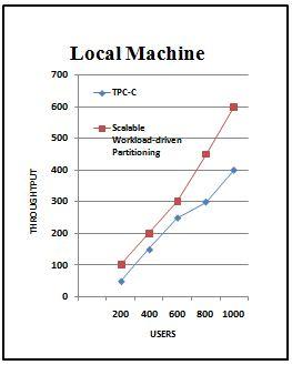
Data Partitioning in Mongo Db with Cloud (Aakanksha Jumle)



ISSN: 2252-8814

Figure 4. Response Time with 15 warehouses on local

Figure 5. Response Time with 15 warehouses on cloud

Figure 6. Throughput with 15 warehouses on local

Figure 7. Throughput with 15 warehouse on cloud

Figure 8. Response Time with 25 warehouses on local

Figure 9. Response Time with 25 warehouses on cloud

IJAAS Vol. 7, No. 1, March 2018: 21 – 28

IJAAS

ISSN: 2252-8814



Figure 10. Throughput with 25 warehouses on local

Figure 11. Throughput with 25 warehouses on cloud

Figure 12. Response Time with 35 warehouses on local

Figure 13. Response Time with 35 warehouses on local

Figure 14. Throughput with 35 warehouses on local

Figure 15. Throughput with 35 warehouses on cloud

Data Partitioning in Mongo Db with Cloud (Aakanksha Jumle)



ISSN: 2252-8814

CONCLUSION Scalable workload-driven partitioning is implemented using MongoDB to satisfy the demands of latest cloud related applications. The experiment performed with the solution of using the workload-driven algorithm is validated over the local machine and also on the cloud. The use of EC2 cloud instance improves the metrics used for validation. By implementing the concerned scheme using the benchmark TPC-C, it has been observed that scalable workload driven partitioning reduces the number of distributed transactions and gives better response time as compared to TPC-C.

REFERENCES [1] Francisco Cruz, Francisco Maia, Rui Oliveira and Ricardo Vila¸ca. Workload-aware table splitting for NoSQL. SAC’14 March 24–28, Gyeongju, Korea Copyright 2014 ACM 978- 1-4503-2469-4/14/03, 2014. [2] S. Ahirrao and R. Ingle, “Scalable Transactions in Cloud Data Stores,” Journal of Cloud Computing: Advances, Systems and Applications, 4:21. DOI 10.1186/s13677-015- 0047-3, 2015. [3] S. Phansalkar and Dr. A. Dani, “Transaction Aware Vertical Partitioning of Database (TAVPD) For Responsive OLTP Applications In Cloud Data Stores,” Journal of Theoretical and Applied Information Technology, Volume. 59 No.1, January 2014. [4] Das S, Agrawal D, El Abbadi A, “ElasTraS: An elastic, scalable, and self-managing transactional database for the cloud”. ACM Trans DatabaseSyst (TODS) 38(Article 5):1–45, 2013. [5] Baker J, Bond C, Corbett J, Furman JJ, Khorlin A, Larson J, L´eon J-M, Li Y, Lloyd A, Yushprakh V, “Megastore: Providing scalable, highly available storage for interactive services”. In: CIDR, Volume 11. pp 223–234, 2011. [6] Miguel Liroz-Gistau, Reza Akbarinia, Esther Pacitti, Fabio Porto and Patrick Valduriez. “Dynamic WorkloadBased Partitioning Algorithms for Continuously Growing Databases”. Springer-Verlag Berlin Heidelberg, 2013. [7] Curino C, Jones EPC, Popa RA, Malviya N, Wu E, Madden S, Zeldovich N, “Relational cloud: A database-as-aservice for the cloud”. In: Proceedings of the 5th Biennial Conference on Innovative Data Systems Research. pp 235–240, 2011. [8] Xiaoyan Wang, Xu Fan, Jinchuan Chen and Xiaoyong Du. “Automatic Data Distribution in Large-scale OLTP Applications”. International Journal of Database Theory and Application. Volume.7, No.4, pp. 37-46, 2014. [9] Curino C, Jones E, Zhang Y, Madden S, “Schism: a workload-driven approach to database replication and partitioning”. Proc VLDBEndowment. 3(1–2):48–57, 2010. [10] Brian Sauer and Wei Hao, “Horizontal Cloud Database Partitioning with Data Mining Techniques”. 12th Annual IEEE Consumer Communications and Networking Conference (CCNC), 2015.

IJAAS Vol. 7, No. 1, March 2018: 21 – 28

International Journal of Advances in Applied Sciences (IJAAS) Vol. 7, No. 1, March 2018, pp. 29~37 ISSN: 2252-8814, DOI: 10.11591/ijaas.v7.i1.pp29-37



Graph Based Workload Driven Partitioning System by Using MongoDB Arvind Sahu, Swati Ahirrao Department of Computer Engineering, Symbiosis International University, India

Article Info

ABSTRACT

Article history:

The web applications and websites of the enterprises are accessed by a huge number of users with the expectation of reliability and high availability. Social networking sites are generating the data exponentially large amount of data. It is a challenging task to store data efficiently. SQL and NoSQL are mostly used to store data. As RDBMS cannot handle the unstructured data and huge volume of data, so NoSQL is better choice for web applications. Graph database is one of the efficient ways to store data in NoSQL. Graph database allows us to store data in the form of relation. In Graph representation each tuple is represented by node and the relationship is represented by edge. But, to handle the exponentially growth of data into a single server might decrease the performance and increases the response time. Data partitioning is a good choice to maintain a moderate performance even the workload increases. There are many data partitioning techniques like Range, Hash and Round robin but they are not efficient for the small transactions that access a less number of tuples. NoSQL data stores provide scalability and availability by using various partitioning methods. To access the Scalability, Graph partitioning is an efficient way that can be easily represent and process that data. To balance the load data are partitioned horizontally and allocate data across the geographical available data stores. If the partitions are not formed properly result becomes expensive distributed transactions in terms of response time. So the partitioning of the tuple should be based on relation. In proposed system, Schism technique is used for partitioning the Graph. Schism is a workload aware graph partitioning technique. After partitioning the related tuples should come into a single partition. The individual node from the graph is mapped to the unique partition. The overall aim of Graph partitioning is to maintain nodes onto different distributed partition so that related data come onto the same cluster.

Received May 24, 2017 Revised Jan 18, 2018 Accepted Feb 11, 2018 Keywords: Graph Partitioning, NoSQL Database, Online Transaction Processing (OLTP), Scalability TPC-C benchmark,

Corresponding Author: Swati Ahirrao, Department of Computer Engineering, Symbiosis International University, Pune, India. Email: swatia@sitpune.edu.in

INTRODUCTION Nowadays, data is generated by their sources is very huge in volume that is called as Big-Data. The companies need a strong foundation for Big-Data handling. So many companies giving more importance to NoSQL database as compare to traditional relational database because relational databases are unable to scale and lack of flexibility. Relational databases also cannot handle globally massive amounts of unstructured data. So it is required to store and process that huge amount of data by using NoSQL database. NoSQL database is persistence solution in the world of Big Data. NoSQL database is more suitable as compare to RDBMS in terms of scalability, volume, variety and efficiency. NoSQL database is capable to handle all type of data like structured, semi-structured, and unstructured data.

Journal homepage: http://iaescore.com/online/index.php/IJAAS



ISSN: 2252-8814

To achieve scalability in NoSQL the data should be partitioned and then distribute those partitions to the different geographically available servers. Partitioning is the most effective technique which is used to access scalability in a system. Scalability is to process the entire generated workload at the defined time boundaries for an application that is running on a number of server nodes. Some most commonly used partitioning techniques are round-robin partitioning, range partitioning and hash partitioning. In round-robin partitioning, each tuple is uniformly distributed to an alternate partition. In range partitioning, the tuples are partitioned according with a range of partition key. In hash partitioning, the tuples are partitioned by using hash key. But these partitioning methods are not efficient for the small workload transactions that access a less number of tuples. Round-robin partitioning, range partitioning and hash partitioning methods are unable to represent sensible n-to-n relationship between tuples. For example social networking like Facebook data appear with the n-to-n relationships that is hard to partitioning by using round-robin partitioning, range partitioning and hash partitioning methods. Sometimes the related tuples come into different partition and unrelated tuples come under same partition which is root cause of distributed transaction. In Fine-Grained partitioning, related individual tuples are combined together in the same partition to reduce the distributed transaction but lookup table is very expensive because of its size. In case of Many-to-many relationship it is hard to partition by using Fine-Grained partitioning. ElasTras [1] used schema level partitioning to improve scalability. In ElasTras Scalability is achieved by the execution of transactions onto the multiple partitions. ElasTras also not formed effective partitions. In Spectral partitioning methods [2-3], partitions produced are effective but very expensive because they require the computation of eigenvector corresponding to the fiedler vector. In Geometric partitioning algorithms [4], are very fast to perform partitions but formed partitions quality are worse than partitions of Spectral partitioning. The web applications and websites of the enterprises are accessed by a huge number of users with the expectation of reliability and high availability. Social networking sites are generating the data in very huge amount and at very fast rate, so to handle that data we need of both computer software scalability and hardware scalability. The concept behind partitioning or shading is to spread data of a table across numerous partitions. Partitioning techniques should be picked up appropriately so that after partitioning the result become more accurate and effective. When data is stored in SQL data bases, it can be partitioned to provide efficiency and scalability. Data partitioning is possible in SQL data store but SQL data stores are unable to partition the data based on relationship. In SQL data partitioning increases the multisite/distributed transactions because sometimes related rows come into different partition. Hence, it is necessary to find an effective partitioning technique, which will consider the relativity among the tuples or data at the time of partitioning. In proposed system, Schism [5] approach is used for partitioning the NoSQL data base. Schism is a workload driven approach for data partitioning. In Schism for Graph Partitioning METIS [2] algorithm is used. METIS provides balanced partitions after partitioning the data. Proposed system improves Scalability and reduces the number of Distributed transactions. With the goal to acquire ideal data placement method in different partitions, here numerous workload-aware partitioning and load balancing techniques have been examined. Graph partitioning technique is easy to understand and the relation between data can represent effectively in the form of Graph. In the Graph database, the nodes represent the database tuples and nodes are connected by an edge if two or more nodes are participating in the same transaction. Graph based workload aware partitioning technique is basically applied for scalability but sometimes if the data partitions are not formed appropriately then it leads to the expensive distribute transactions. Here expensive in terms of response time and resource utilization or network usage. So to overcome the problem of expensive distributed transactions min-cut k balanced partitions come into the picture. In min-cut balanced partitions, data partitioning happens based on some relation that data contains, which minimize the multisite/distributed transactions. After partitioning the database, the decision tree classifier techniques are applied to extract the set of rules based on that rules data is partitioned. When scalability improves then maintenance of data becomes easy and time taken to process a query reduces. Ultimately, along with the scalability performance also increases. The rest of the paper is organized as follows: in Section 2, papers related to scalability and graph database partitioning is discussed. Section 3 gives Brief overview of proposed system. In Section 4, Design of graph based workload driven partitioning system is presented. In Section 5, Implementation details explain implementation and the performance evaluation of the partitioning system. In Section 6 and Section 7, experimental setup and results are described respectively. Finally in Section 8 conclusion of the paper.

IJAAS Vol. 7, No. 1, March 2018: 29 – 37

IJAAS

ISSN: 2252-8814



RELATED WORK Scalable database and distributed database is emerging and interested topic for the database research group. Accordingly, many techniques for scalable database transaction are already present. In this chapter, all the existing partitioning algorithms and graph partitioning techniques are discussed. Curino [5] have proposed Schism technique for database replication and partitioning for OLTP databases. Schism is a data driven graph partitioning algorithm which improves the scalability of the system. Schism uses METIS algorithm for partitioning the graph. Schism formed the balanced partitions that reduce the number of distributed transactions. K-way partitioning algorithm is used to find refined partition in METIS. K-way applies for further partitioning the data that reduces the effect of distributed transactions and increases the throughput. Schism provides good partitioning performance and easy to integrate into existing databases. In Schism representation of n-to-n relationship effectively and allow multiple schema layouts. Schism is a better approach for replication and partitioning of social networking data. In Schism workload changes can affect the performance and aggressive replication is used. Karypis [6] have proposed METIS which follows Multilevel Graph Partitioning. METIS is an open source graph partitioning technique. In Multilevel graph partitioning there are three phases. Firstly, in graph coarsening phase the graph developed by incoming workload is partitioned. Second, in initial partitioning the graphs are further partitioned into the small graphs for refinement. Initial partitioning produces the balanced partitions. Third, in un-coarsening is for rebuilding the final graph after refinement. METIS is fast as compare to other partitioning algorithm. METIS provides quality of partitions and required less memory because of dynamic memory allocation. In METIS, we cannot major exact amount of required memory. Tatarowicz [7] have proposed Fine-Grained Partitioning for distributed database. In proposed partitioning approach related individual tuples are combined together in the same partition. Lookup table used to maintain a smooth partitioning because it is needed to store the location of each tuple. The lookup table stores location of each tuple that acts as a metadata table. Many-to-many relationship is hard to partition because number of distributed transactions increase in case of Many-to-many relationship. In Fine-Grained partitioning the number of distributed transactions can be reduced by well assignment of tuples to each partition. It reduces the main memory consumption and improves the performance. Sometimes to maintain Fine Grained Partitioning routing (Lookup) tables is very expensive because of its size. Quamar [8] have proposed Scalable Workload-Aware Data partitioning for Transactional data processing. Hypergraph is used to represent the workload and reduces the overheads of partitioning by hyperedge. Overheads happen at the time of data placement or query execution at runtime that is reduces by SWORD technique. Workload changes are handled by incremental data repartitioning technique. For high availability it uses active replication technique. By Active replication number of distributed transactions reduces, accessibility increases and load balancing can be accessed. SWORD is used to minimize the cost of distributed transactions. SWORD represents data in compressed format so number of generated partitions would be minimal. Lu Wang [9] have proposed a Multi-level Label Propagation (MLP) method for partitioning of the graph. All the web users are represented on the graph. If graph partitioned efficiently then load balancing becomes easy and less communication overhead. The quality of generating partitions by MLP approach is compared to the small size graph. To evaluate quality of the formed partitions it is compared to METIS. In MLP formed partitions are good with respect to time and memory. MLP are more effective and scalable partitioning which can scale up to billions of nodes. MLP algorithm cannot use for general-purpose. Chris [10] have proposed a Min-max Cut algorithm. Aim of Min-Max is to increase number of similar nodes within a cluster and reduce the number of similar nodes between different clusters. Similar nodes between two sub-graphs should be less. Similar nodes within each sub-graph should be higher. Minmax cut is used to improve the clustering accuracy and gives an optimal solution. Tae-Young [11] have proposed k-way Graph Partitioning Algorithm to reduce the size of the graph. The recursive spectral bisection method reduces the size of the graph by the breaking edges and vertices. The recursive spectral bisection method is used for clustering small graph in a k-way. Balancing constraints should maintain to all partitions of graphs. In Multi-Level Partitioning for recursive partitioning k-way algorithm is used. K-way takes less time to partition the graph. K-way is a good option for partitioning small graphs only. Dominique [12] introduce Parallel Hill-Climbing algorithm for graph partitioning. This algorithm is used for share memory for refinement algorithm parallel. Hill-climbing takes imaginary move on different vertices so that it can find new local minima. The refinement algorithm produces high-quality partitioning. Hill-Scanning is the refinement algorithm for refining k-way partition. Hill-Scanning has better performance than other parallel refinement algorithm. Hill-Scanning it is much faster and provides better quality partition.

Graph Based Workload Driven Partitioning System by Using MongoDB (Arvind Sahu)



ISSN: 2252-8814

Maria [13] introduces a new shared memory parallel algorithm that is Coupling-Aware Graph Partitioning Algorithm. Coupling-Aware is used to produce high-quality partitions as compared to the k-way partitioning algorithm. Co-partitioning allows scalability in term of processing unit. In Coupling-aware partitioning there is no need to partition codes independently or separately. It can reuse available codes through a coupling framework without combining them into a standalone application. Coupling –Aware reduces the coupling communications costs. Coupling-Aware provides better global graph edge cut. James [14] have proposed Simulated Bee Colony Algorithm to partition the graph. Simulated Bee Colony is totally inspired by the foraging behavior of honey bees. In SBC algorithm the partial result can be reused further if compatible in a scenario. SBC produces very high quality of partitions. SBC is used when the quality is most important and performance can be moderate. SBC algorithm is not suitable for real-time applications. SBC performance is low that is why parallel processing is not possible

PROPOSED SYSTEM OVERVIEW In our proposed system, Firstly system stores the data in NoSQL database that is MongoDB and then represents that data in the form of graph by using Neo4j. Graph representation is necessary for easy understanding where tuples are represents as node and transaction represent by edge. Graph partitioning technique is applied to find the minimum cut balanced partition so that the distribute relation between nodes should be minimal. Finally, the Decision tree classifier is applied to develop some sort of rules to take decision regarding partition strategy. On these rules the partition of data depends. Here Schism approach is used for partitioning the data. Schism is a workload driven approach for database partitioning. In Workload driven partitioning systems, the partition of data happens based on some relation between data. The relation found based on access patterns. In transaction, the data that is mostly accessed together contains high relation, so related data comes into a single partition of database. The architecture of the proposed system “Graph based workload driven partitioning system” is shown in figure. Our proposed system is designed to work as a Scalable transactional system on the top of distributed storage system. Here MongoDB is distributed storage system which implements CRUD (Create/Insert, Read, Update and Delete) operations. Administrator Node is the actual server which performs partitioning by using the algorithm here Schism is using to partition the data. Shannon Information gain is calculated to find the relation between the data. Decision tree decides migration of data. Backend database is MongoDB. MongoDB is a NoSQL database store, which actually contains the data.

Figure 1. System Architecture

In our proposed system, the input is workload trace and a number of partitions required and the output is the balanced partitions. Because of balanced partitions the number of distributed transaction reduces and performance increases

IJAAS Vol. 7, No. 1, March 2018: 29 – 37

IJAAS

ISSN: 2252-8814



3.1. Partition the Graph After Graph representation, the Graph partitioning algorithm is applied to partition the Graph. Balanced partitions formed after Graph partitioning. Each particular node/tuple belongs to a database partition and each database partition allocate to a physical separated node. 3.2. Shannon Information Gain Shannon information gain is needed for effective classification or partition of database. Shannon information gain is used to calculate the entropy/impurity of the data. Decision tree takes decision based on Shannon information gain. If two tuples has nearer Shannon information gain it means they contain some relation and come into a single partition. 3.3. Distributed Transactions In Distributed system, the transactional data available at the different physical locations. The distribution of data should be based on some analysis or relation might reduce the number of distributed transaction. Practically Distributed systems are good choice because it provides transparency, scalability and high performance.

GRAPH BASED WORKLOAD DRIVEN PARTITIONING ALGORITHM In proposed system, Schism Approach is using for partitioning the graph. Schism approach works in five steps. 4.1. Data Pre-processing Phase

4.2. Graph Representation Phase Big data is being generated by web applications. Graph representation of data provides a proper and easy understanding, mapping and relation between data. After the data pre-processing step, whole data or workload trace is represented in the form of Graph. Each node represents a tuple and an edge represents the frequency of tuples within a transaction. Nodes, which are accessed in the same transaction is connected by an edges. 4.3. Graph Partitioning Phase In this phase, partitioning of the graph performed. Metis Algorithm psuedcode-Metis algorithm works in three steps: a. Coarsening- During the Coarsening phase, merging of node until the small graph is formed. b. Initial partitioning- During the Initial partitioning phase, k-way partitioning of the smaller graph is computed. c. Un-coarsening phase- During the Un-coarsening phase, refined partitions are formed after refinement. 4.4. Explanation Phase In this phase, create the rules and store that rules into database. Based on these rules decision are taken. Find a compact model that captures the (tuple; partition) mappings produced by the partitioning phase. Use decision trees to produce understandable rule-based output. These rules are combination of tuple and partition (tuple: partition). That describes the tuple and stored location. 4.5. Validation Phase

IMPLEMENTATION DETAILS Calculate Shannon Information Gain: Here in this step distribution factor of the input parameters are analyzed by using Shannon information gain. Shannon information gain yields distribution entity in between 0 and 1. Any values that are nearer to 1, is always consider as the highly distributed factor and it is consider as the most important factor. So this step applies info gain method on clustered data from graph based on the user and warehouse to check for the probability of the highest order warehouse with respect to the input data. For this purpose system uses the Shannon information gain theory which can be state with the help of the following equation 1: IG( E ) = - (P / T ) log (P / T ) - ( N / T ) log (N / T )

(1)

Graph Based Workload Driven Partitioning System by Using MongoDB (Arvind Sahu)



ISSN: 2252-8814

where P N T IG (E)

= Frequency of the warehouse entity’s present count in the clusters = Non presence count = Total number of clusters = Information Gain for the given Entity On applying this equation, that yields the value in between 0 to 1. The data size, that are having value nearer to 1 indicating the highest priority in the list. Develop Decision Tree: Decision Tree extract some rules based on Shannon information gain and take decision based on that rules. Based on the graph partition clusters and Shannon information gain decision tree is created. After decision tree creation a matrix will create for the decision protocols. Matrix contains optimized routing partitioned data with respect to the warehouses. This can be representing with the following algorithm 1. Algorithm 1: Generate Decision Tree (db, p):dt // F1, F2, F3 are fitness functions Step 0: Start Step 1: While stop criterion is not met Step 2: Evaluate fitness of dt attribute it to F1 Step 3: Perform x mutations to Storage Nodes Step 4: Store F1 into F2 Step 5: While j<number of mutations to Prediction Nodes Step 6: Select and mutate a node Step 7: Evaluate fitness F3 of mutated tree Step 8: If F3>F2 Step 9: Accept mutated tree Step 10: Attribute F3 to F2 Step 11: End-if Step 12: End-While Step 13: If F2>F1 Step 14: Attribute resulting tree to dt Step 15: Attribute F2 to F1 Step 16: End-If Step 17: End-While Step 18: Return dt Step 19: Stop

EXPERIMENTAL SETUP To implement the proposed system java programming language and java-based NetBeans IDE is used. For experimental prove three hardware separated machines are considered that have core i3 processor with 4GB of RAM. Here three Hardware separated machines are used for the distributed paradigm. Proposed System uses NoSQL MongoDB for the graph-based workload driven partitioning system. To stimulate the transactional workload in the form of graph the Neo4j graph database is used. The response time of developed system is validating by using TPC-C benchmark.

RESULT Proposed system uses Mongo DB NoSQL database for the experiment. The developed system put under hammer in many scenarios to prove its authenticity as mentioned in below tests. To evalute performance of the system response time, throughput and number of distributed transactions are considering. When the system is subjected to get the throughput for 10 warehouses an experiment is conducted to get the same, whose result is tabulated in Table 1

IJAAS Vol. 7, No. 1, March 2018: 29 – 37

IJAAS



ISSN: 2252-8814

Table 1. Throughput and Time Response for 10 Warehouse No of Transcations

Single DB Time in Seconds

Multiple DB Time in Seconds

20 40 60 80

8.547 18.789 26.771 37.44

5.47 8.482 15.774 20.475

Throughput for Single DB (No of Transactions per Seconds 2.34000234 2.12890521 2.241231183 2.136752137

Throughput for Multiple DB (No of Transactions per Seconds 3.65630713 4.715868899 3.803727653 3.907203907

When a plot is drawn for this throughput results we get some interesting facts that can be seen Figure 3. Where we can observer that throughput is increased sweepingly for the multiple DB transactions. That means on distribution of the databases number of transactions per second will increase to yield better results

Figure 2. Time Delay Comparison for 10 Warehouses

Figure 3. Throughput Comparison for 10 Warehouses

When the system is subjected to get the throughput for 15 warehouses an experiment is conducted to get the same, whose result is tabulated in Table 2.

Table 2. Throughput and Time Response for 15 Warehouses No of Transcations

Single DB Time in Seconds

Multiple DB Time in Seconds

20 40 60 80

8.78 17.77 21.58 34.25

4.98 7.87 13.5 16.52

Figure 4. Time Delay Comparison for 15 Warehouses

Throughput for Single DB (No of Transactions per Seconds 2.277904328 2.250984806 2.780352178 2.335766423

Throughput for Multiple DB (No of Transactions per Seconds 4.016064257 5.082592122 4.444444444 4.842615012

Figure 5. Throughput Comparison for 15 Warehouses

Graph Based Workload Driven Partitioning System by Using MongoDB (Arvind Sahu)



ISSN: 2252-8814

When the system is subjected to get the throughput for 20 warehouses an experiment is conducted to get the same, whose result is tabulated in Table 3.

Table 3. Throughput and Time Response for 20 Warehouses No of Transcations

Single DB Time in Seconds

Multiple DB Time in Seconds

20 40 60 80

7.44 15.66 19.22 32.02

4.4 7.01 11.2 15

Figure 6. Time Delay Comparison for 20 Warehouses

Throughput for Single DB (No of Transactions per Seconds 2.688172043 2.554278416 3.121748179 2.498438476

Throughput for Multiple DB (No of Transactions per Seconds 4.545454545 5.706134094 5.357142857 5.333333333

Figure 7. Throughput Comparison for 20 Warehouses

When the system is subjected to get the throughput for 25 warehouses an experiment is conducted to get the same, whose result is tabulated in Table 4.

Table 4. Throughput and Time Response for 25 Warehouses No of Transcations

Single DB Time in Seconds

Multiple DB Time in Seconds

20 40 60 80

6.21 12.1 17.2 29.2

2.2 6.4 10.24 13

Figure 8. Time Delay Comparison for 25 warehouses

Throughput for Single DB (No of Transactions per Seconds 3.220611916 3.305785124 3.488372093 2.739726027

Throughput for Multiple DB (No of Transactions per Seconds 9.090909091 6.25 5.859375 6.153846154

Figure 9. Throughput comparison for 25 warehouses

CONCLUSION In proposed algorithm, graph based workload driven partitioning system for NoSQL database is presented. Workload is represented in the form of graph to take the advantage of the relationship between data. Based on that relationship tuples are combined together into a single partition. Partitioning based on IJAAS Vol. 7, No. 1, March 2018: 29 – 37

IJAAS

ISSN: 2252-8814



relation reduces the number of distributed transactions and increase Throughput. TPC-C benchmark is used for validation of proposed system. Proposed system improves the response time and throughput, which is considerably less than the TPC-C schema. Hence, proposed approach shows better results in terms of distributed transactions and throughput.

REFERENCES [1] Das, Sudipto, Divyakant Agrawal, and Amr El Abbadi. "ElasTraS: An elastic, scalable, and self-managing transactional database for the cloud." ACM Transactions on Database Systems (TODS) 38.1: 5, 2013. [2] Alex Pothen, H. D. Simon, Lie Wang, and Stephen T. Bernard. “Towards a fast implementation of spectral nested dissection”. In Supercomputing ’92 Proceedings, pages 42–51, 1992. [3] Alex Pothen, Horst D. Simon, and Kang-Pu Liou. “Partitioning sparse matrices with eigenvectors of graphs”. SIAM Journal of Matrix Analysis and Applications, 11(3):430–452, 1990. [4] Gary L. Miller, Shang-Hua Teng, and Stephen A. “Vavasis. A unified geometric approach to graph separators”. In Proceedings of 31st Annual Symposium on Foundations of Computer Science, pages 538–547, 1991. [5] Curino, Carlo, et al. "Schism: a workload-driven approach to database replication and partitioning." Proceedings of the VLDB Endowment 3.1-2: 48-57, 2010. [6] Karypis, George, and Vipin Kumar. "METIS unstructured graph partitioning and sparse matrix ordering system, version 2.0.", 1995. [7] Tatarowicz, Aubrey L., et al. "Lookup tables: Fine-grained partitioning for distributed databases." 2012 IEEE 28th International Conference on Data Engineering.IEEE, 2012. [8] Quamar, Abdul, K. Ashwin Kumar, and AmolDeshpande. "SWORD: scalable workload-aware data placement for transactional workloads." Proceedings of the 16th International Conference on Extending Database Technology.ACM, 2013. [9] Wang, Lu, et al. "How to partition a billion-node graph." 2014 IEEE 30th International Conference on Data Engineering.IEEE, 2014. [10] Ding, Chris HQ, et al. "A min-max cut algorithm for graph partitioning and data clustering." Data Mining, 2001.ICDM 2001, Proceedings IEEE International Conference on IEEE, 2001. [11] Choe, Tae-Young, and Chan-Ik Park. "A k-way graph partitioning algorithm based on clustering by eigenvector." International Conference on Computational Science. Springer Berlin Heidelberg, 2004.APA. [12] LaSalle, Dominique, and George Karypis. "A Parallel Hill-Climbing Re_nement Algorithm for Graph Partitioning." 2015. [13] Predari, Maria, and Aur_elienEsnard. "Coupling-aware graph partitioning algorithms: Preliminary study." 2014 21st International Conference on High Performance Computing (HiPC). IEEE, 2014. [14] McCa_rey, James D. "Graph partitioning using a Simulated Bee Colony algorithm." Information Reuse and Integration (IRI), 2011 IEEE International Conference on IEEE, 2011.

Graph Based Workload Driven Partitioning System by Using MongoDB (Arvind Sahu)

International Journal of Advances in Applied Sciences (IJAAS) Vol. 7, No. 1, March 2018, pp. 38~45 ISSN: 2252-8814, DOI: 10.11591/ijaas.v7.i1.pp38-45



A Fusion Based Visibility Enhancement of Single Underwater Hazy Image Samarth Borkar, Sanjiv V. Bonde Department of Electronics and Telecommunication Engineering, Shri. Guru Gobind Singhji Institute of Engineering and Technology, SRTMUN University, India

Article Info

ABSTRACT

Article history:

Underwater images are prone to contrast loss, limited visibility, and undesirable color cast. For underwater computer vision and pattern recognition algorithms, these images need to be pre-processed. We have addressed a novel solution to this problem by proposing fully automated underwater image dehazing using multimodal DWT fusion. Inputs for the combinational image fusion scheme are derived from Singular Value Decomposition (SVD) and Discrete Wavelet Transform (DWT) for contrast enhancement in HSV color space and color constancy using Shades of Gray algorithm respectively. To appraise the work conducted, the visual and quantitative analysis is performed. The restored images demonstrate improved contrast and effective enhancement in overall image quality and visibility. The proposed algorithm performs on par with the recent underwater dehazing techniques.

Received May 21, 2017 Revised Jan 23, 2017 Accepted Feb 11, 2018 Keyword: Color constancy Contrast enhancement Image dehazing Image fusion Underwater image restoration

Corresponding Author: Samarth Borkar, Computer Vision and Pattern Recognition lab. Department of Electronics and Telecommunication Engineering, Shri. Guru Gobind Singhji Institute of Engineering and Technology, Vishnupuri - Nanded, Maharashtra, 431606, India. Email: borkarsamarth@sggs.ac.in

INTRODUCTION Underwater images are inherently dark in nature are also plagued by various small suspending particles and marine snow in an aqueous medium. To increase the visibility range and vision depth, an artificial light is utilized. The rays of light are scattered by particles in the underwater medium and along with color attenuation results in problems such as contrast reduction, blurring of an image and color loss driving the images beyond recognition. For underwater applications such as observation of the oceanic floor, monitoring of fish, study of coral reef etc. demands dehazing of images so as to recover color, enhance visibility and increase visual details present in the degraded image for computer vision and object recognition. In absence of any dehazing technique, the performance and usability of a standard enhancement algorithm may fail to produce desirable results. Basically, dehazing is a process to restore the contrast of an image. Traditional approaches like histogram equalization, histogram specification, and various other contrast enhancement techniques do not deliver desired output images. Over the last few years, diverse techniques have been proposed to restore the underwater hazy images. The dehazing approaches can be grouped into software based and hardware based. Hardware based techniques refer to utilization of polarization filter [1], range gated imaging [2] and using multiple underwater images [3], whereas software based techniques are further grouped into a physical model based and non-physical models. In physical model underwater image processing, parameters of the model are estimated and then restoration is achieved. Estimating the depth of underwater haze is the major hindrance in such models. Journal homepage: http://iaescore.com/online/index.php/IJAAS

IJAAS

ISSN: 2252-8814



Recently physical model-based techniques have gained wide attention. A pioneering work in this direction by He et al., based on dark channel prior (DCP) using minimum pixel intensity for each of the three channels in local patches to obtain the depth of haze changed the future course of research in image dehazing [4]. Carlevaris-Bianco et al. proposed dehazing based on the attenuation difference between RGB color channels [5]. Chiang and Chen presented wavelength compensation and dehazing based on modified DCP [6]. Following this method, underwater image restoration using joint trilateral filter [7], based on least attenuating color channel [8], contrast enhancement for underwater turbid images [9] was presented. But still, underwater dehazing based on the physical foundation from an original image is a challenging problem owing to statistical prior assumptions. Methods based on the non-physical model are presented by various researchers. Integrated color model based underwater image enhancement is presented in [10] and unsupervised color correction technique based on histogram stretching and color balance was proposed in [11]. Bazeille et al. proposed series of filters to enhance contrast, adjust colors and suppress noise [12]. Ancuti et al. presented inspiring work in the field of underwater image enhancement using Laplacian pyramid decomposition thereby increasing contrast [13]. In this method, two inputs to fusion framework are derived from the original underwater image using white balancing technique and color correction technique applied to single hazy underwater images. Weights for the fusion process included Laplacian contrast, local contrast, Saliency and degree of exposedness. A method based on Retinex was proposed by Fu et al. to handle blurring and underexposure of underwater images [14]. Sheng et al. restored blurred and defocussed underwater images using Biorthogonal wavelet transform [15]. Amidst all these underwater dehazing algorithms it is arduous to pick the best of the available algorithms on account of the absence of ground truth images. There is an inherent need for creation of a standard database in underwater imaging science. Our strategy is based on multiresolution DWT fusion framework. The two inputs to fusion are derived using effective contrast enhancement algorithm and robust color constancy algorithm. The fused image is then subjected to contrast stretching operation to improve the global contrast and visibility of dark regions. The remainder of this article is as organized. In Section 2, we describe the proposed underwater dehazing algorithm in detail regarding the choice of selection of color constancy algorithm, discrete wavelet transform (DWT) fusion, and color enhancement. In Section 3, we report the outcomes of qualitative and quantitative analysis and lastly, conclusions are outlined in Section 4.

PROPOSED RESEARCH METHOD In this paper, we propose the enhancement of single underwater images based on multiresolution DWT fusion. We generate the two inputs for the fusion framework from contrast enhanced and color constancy algorithm from the original input image. The restoration of the hazy image is strongly dependent on the selection of inputs. The need for the selection of these two inputs is as explained in following subsections. The block diagram of the proposed algorithm is as shown in Figure 1.

Figure 1. Schematic Diagram of Proposed Algorithm for Single Underwater Image Enhancement

2.1 Obtaining Contrast Enhanced Image Underwater images suffer from low contrast due to diminished illumination. The traditional contrast enhancement techniques exhibit severe limitations in underwater imaging. So in this work we adopted and A Fusion based Visibility Enhancement of Single Underwater Hazy Image (Samarth Borkar)



ISSN: 2252-8814

modified SVD and DWT based technique as presented in [16]. We target illumination component of the underwater image. We apply contrast enhancement to DWT LL sub-band of V plane using the SVD and DWT combinational method to solve the problem of low contrast. This illumination information is exhibited in singular value matrix of SVD. We modify the coefficients of singular value matrix to obtain desired enhancement in illumination component and other details in SVD are not altered. Also, in the underwater scenario, the formation of haze is a uniform intensity function, and the haze affected areas have analogously more brightness. This makes wavelet or scale space representation as provided by DWT, a useful tool to model hazy regions. The approximation coefficients (LL sub-band) correlates to localized haze information, whereas detail coefficients (LH, HL, and HH) embed edge information. So by applying the enhancement operation only on LL sub-band results in enhanced image with sharp edges. In our presented work, we have applied contrast enhancement technique using SVD and DWT on V channel of HSV color space, thereby not affecting the color composition of original input hazy image. The V channel is processed by histogram equalization to obtain vHE. The two images V and vHE are decomposed by DWT in four sub-bands. The singular value matrix correction coefficient is obtained using the equation:

𝜉=

max(𝛴𝐿𝐿𝑣𝑣𝑣 ) max(𝛴𝐿𝐿𝑣 )

(1)

where 𝛴𝐿𝐿𝑣 and 𝛴𝐿𝐿𝑣𝑣𝑣 are SVD values of the input image and the resulting image of the histogram equalized technique. The modified LL band is given by:

�� 𝛴 𝐿𝐿𝑣 = 𝜉. 𝛴𝐿𝐿𝑣

�� 𝐿𝐿𝑣 = ∪𝐿𝐿𝑣 . 𝛴 𝐿𝐿𝑣 . 𝑉𝐿𝐿𝑣

(2) (3)

��𝑣 , 𝐿𝐿𝑣 , 𝐻𝐻𝑣 and 𝐻𝐻𝑣 sub-bands, the new equalized V channel image is generated By applying IDWT to 𝐿𝐿 ��𝑣 , 𝐿𝐿𝑣 , 𝐻𝐻𝑣 , 𝐻𝐻𝑣 ) (4) 𝑉� = IDWT (𝐿𝐿

The 𝑉� component is then concatenated with H and S component in HSV color space to obtain contrast enhanced RGB image. 2.2. Obtaining White Balanced Image Apart from diminished contrast problems, underwater images are prone to color loss attributed to wavelength attenuation [17]. Also, due to an artificial source of light at appreciable depth, unwanted color casts arises. Turbidity is not a big problem at deeper depths as compared to shallow waters due to the absence of marine snow and no appreciable underwater flow movement. So white balancing technique is a necessity. A large number of white balancing techniques are available in the literature [18]. We tried, white patch algorithm, MaxRGB algorithm, Gray-Edge algorithm [19] and Shades of Gray algorithm [20]. We obtained the best possible results for Shades of Gray algorithm. As listed in [13] the probable reasons for the failure of white patch algorithm are attributed to limited specular reflection and failure of Gray Edge algorithm is on account of low contrast and diminished edges as compared to outdoor images. Finlayson and Trezzi presented shades of Grey algorithm based on the assumption that image scene average is a function of some shades of Grey. It calculates the weighted average of the pixel intensity by assigning higher weight to pixel with higher intensity, based on Minkowski-norm p and is given as: 1

∫(𝑓 (𝑥))𝑝 𝑑𝑑 𝑝 � � ∫ 𝑑𝑑

= 𝑘𝑘

(5)

where 𝑓(𝑥) is the input image, 𝑥 is the spatial coordinate in the image and k is constant. Shades of Grey algorithm is trade-off between Gray World (𝑝 = 1) and MaxRGB algorithm (𝑝 = ∞).

2.3. Multimodal Image Fusion Using DWT The wavelet based fusion techniques are widely used in medical image restoration [21], satellite imaging [22], outdoor scene imaging [23] etc. The transform coefficients of DWT are representatives of IJAAS Vol. 7, No. 1, March 2018: 38 – 45

IJAAS



ISSN: 2252-8814

image pixels. It transforms the input series 𝑥0 , 𝑥1 , 𝑥2 … , 𝑥𝑚 into high pass wavelet coefficients and low pass 𝑛 coefficients series of length each given by (6) and (7) 2

𝑘−1 𝑥2𝑖−𝑚 . 𝑠𝑚 (𝑧) 𝐻𝑖 = ∑𝑚=0

(6)

𝑘−1 𝑥2𝑖−𝑚 . 𝑡𝑚 (𝑧) 𝐿𝑖 = ∑𝑚=0

(7) 𝑛

where 𝑠𝑚 (𝑧) and 𝑡𝑚 (𝑧) are called wavelet filters and 𝑖 = 0, … , ( -1) and k is the length of the filter [24][29]. 2 As discussed earlier, there are two components in DWT, approximation, and detail sub-bands. In our application, we propose to fuse contrast enhanced and white balanced image, in order to obtain a dehazed underwater single image. For the approximation sub-bands we use, the corresponding mean coefficients and for retaining edges we use maximum coefficients of the two (contrast enhanced and white balanced) detailed sub-bands. We decompose the first input and second input into individual approximation sub-bands 𝐼1𝑎 and 𝐼2𝑎 where notation 1 and 2 corresponds to first input and second input and a signifies approximation sub-band. Similarly we decompose two input images into 𝐼1𝑑 and𝐼1𝑑 , where d signifies corresponding detail sub-bands (LH, HL and HH). Algorithm for DWT image fusion is as follows: Step 1: Compute approximation coefficient for fused image 𝐼𝑓 , using fusion rule as: 1

𝐼𝑓𝑎 = (𝐼1𝑎 + 𝐼2𝑎 )

(8)

𝐼𝑓𝑑 = 𝑚𝑚𝑚(𝐼1𝑑 , 𝐼2𝑑 )

(9)

𝐼 = 𝑖𝑖𝑖𝑖 �𝐼𝑓𝑎 , 𝐼𝑓𝑑 �

(10)

Step 2: Compute detailed coefficient for fused image 𝐼𝑓 , using fusion rule as: Step 3: Follow Step 1 and Step 2 for the desired level of resolution. Step 4: Reconstruct the enhanced image using inverse discrete wavelet transform as:

This process preserves the dominant features without introducing any artifacts. 2.4. Post-Processing Using Contrast Stretching The image after fusion needs to be post-processed using contrast stretching so as to increase the dynamic range of pixels and enhance contrast. A simplified contrast stretching algorithm [11][30] uses a linear scaling function of the normalized pixel value. The image restored 𝐼𝑅 (𝑥, 𝑦) is given as 𝐼𝑅 (𝑥, 𝑦) = (𝐼(𝑥, 𝑦) − 𝐼𝑚𝑚𝑚 ) �

𝐼𝑑 𝑚𝑚𝑚 −𝐼𝑑 𝑚𝑚𝑚 𝐼𝑚𝑚𝑚 −𝐼𝑚𝑚𝑚

� + 𝐼𝑑 𝑚𝑚𝑚

(11)

where 𝐼𝑅 (𝑥, 𝑦) is the normalized pixel intensity after contrast stretching, 𝐼𝑚𝑚𝑚 is the lowest intensity in the existing image, 𝐼𝑚𝑚𝑚 is the highest intensity in the existing image, 𝐼𝑑 𝑚𝑚𝑚 is the minimum pixel intensity in the desired image and 𝐼𝑑 𝑚𝑚𝑚 is the maximum pixel intensity in the desired image. 3.

EXPERIMENTAL RESULTS AND ANALYSIS As we do not have a ground truth or separate reference image as such, the choice of image assessment for quantitative as well as qualitative analysis becomes a difficult task. Figure 2, shows the histogram of images before and after restoration. It is seen that our proposed method is able to enhance the contrast range. We have compared our proposed methods with contemporary methods such as Ancuti et al. [13], Bazeille et al. [12], Carlevaris et al. [5], Chiang and Chen [6], Galdran et al. [8], and Serikawa & Lu [25]. Of these methods, [5-6] and [25] are based on image restoration model and employ modified dark channel prior as proposed in [4], and [12-13] are representatives of enhancement methods. Our work is based on the non-physical model, but we have compared our work with both restoration as well as enhancement techniques.

A Fusion based Visibility Enhancement of Single Underwater Hazy Image (Samarth Borkar)



ISSN: 2252-8814

3.1. Qualitative Evaluation As shown in Fig 2-5, we have compared our results with the standard methods. It can be seen that our method is able to restore visibility and remove color cast along with [12], [13] and [8] work, whereas in the results of [5], [6], [25], the color and details are not improved. Ancuti et al.’s method remove the haze completely exhibiting optimum visibility but rendering an oversaturated appearance, whereas Bazeille et al.’s method, the color fidelity loss is prominent. The method of Galdran et al. is able to recover and restore the natural appearance of the underwater scene but with lesser brightness as compared to our work. The method of Serikawa and Lu also fails to produce the enhanced visibility, as is the case with Chiang and Chen method.

Figure 2. Visual comparison on image Fish with size 512x384: (a) input image; (b) by [13]; (c) by [12]; (d) by [5]; (e) by [6]; (f) by [25]; (g) by [8]; and (h) with proposed method

Figure 3. Visual comparison on image Coral with size 512x384: (a) input image; (b) by [13]; (c) by [12]; (d) by [5]; (e) by [6]; (f) by [25]; (g) by [8]; and (h) with proposed method

IJAAS Vol. 7, No. 1, March 2018: 38 – 45

IJAAS



ISSN: 2252-8814

Figure 4. Visual comparison on image Shipwreck with size 512x384: (a) input image; (b) by [13]; (c) by [12]; (d) by [5]; (e) by [6]; (f) by [25]; (g) by [8]; and (h) with proposed method

Figure 5. Visual comparison on image Diver with size 512x384: (a) input image; (b) by [13]; (c) by [12]; (d) by [5]; (e) by [6]; (f) by [25]; (g) by [8]; and (h) with proposed method

3.1. Quantitative evaluation For quantitative analysis, we referred to earlier works to select the assessment parameters. We have used quality metrics such as a measure of ability to restore edges & gradient mean ratio of the edges [26], image entropy [21], structural similarity index [27], and PSNR [28]. Table 1 shows the visibility recovery in terms of a measure of ability to restore edges ‘e’ and Table 2 shows the gradient mean ratio of the edges ‘r’.

Table 1: Measure of Ability to Restore Edges ‘e’ Methods Ancuti et al. [13] Bazeille et al. [12] Carlevaris et al. [5] Chiang and Chen [6] Galdran et al. [8] Serikawa and Lu [25] Proposed Method

Fish 1.723 0.928 0.147 0.275 1.276 0.621 1.108

Coral -0.05 -0.11 -0.13 0.025 0.163 -0.01 0.100

Shipwreck 0.462 0.228 0.326 0.070 0.458 -0.02 0.457

Diver 10.34 3.728 0.486 0.839 6.648 1.414 5.483

Table 2: Measure of Gradient Mean Ratio of the Edges ‘r’ Methods Ancuti et al. [13] Bazeille et al. [12] Carlevaris et al. [5] Chiang and Chen [6] Galdran et al. [8] Serikawa and Lu [25] Proposed Method

Fish 4.624 5.939 1.124 1.405 2.202 1.861 2.419

Coral 1.602 3.575 2.872 1.385 1.152 1.662 1.499

Shipwreck 2.972 5.196 2.568 1.992 2.343 2.033 1.401

Diver 4.103 5.264 1.310 1.352 2.081 1.715 1.942

A Fusion based Visibility Enhancement of Single Underwater Hazy Image (Samarth Borkar)



ISSN: 2252-8814

As can be seen in Table 3, the proposed method surpass other methods in terms of entropy. Furthermore, our method performs on par with, Carlevaris et al., Chiang & Chen and Serikawa & Lu in terms of structural similarity index (SSIM). The Peak signal-to-noise ratio, although not the best in the list, still exhibit higher values. The results overall demonstrate that our method works efficiently to remove the underwater haze.

Table 3: Average values in terms of entropy, SSIM, and PSNR Image

Fig. 2 to 5

Methods Ancuti et al. [13] Bazeille et al. [12] Carlevaris et al. [5] Chiang and Chen [6] Galdran et al. [8] Serikawa and Lu [25] Proposed Method

Entropy 7.65 7.50 7.41 7.63 7.57 7.51 7.75

SSIM 0.50 0.19 0.89 0.86 0.29 0.83 0.82

PSNR 21.29 18.72 29.29 27.93 19.40 25.87 24.33

CONCLUSION In this proposed work we have implemented simple yet effective underwater single image enhancement technique to address the problem of visibility restoration and unwanted color cast. The proposed technique has been evaluated for visual and quantitative analysis. Experimental outcome reveals that our results are comparable to and performance wise effective as compared to other recent techniques. The proposed work greatly enhance the visual details in an image, enhance the clarity from a contrast point of view and preserve the natural color without losing image information as observed in state of the art techniques. Also, using this proposed method we are able to overcome the limitations encountered in a patch based underwater image dehazing problems such as computation of atmospheric light value, difficulty with large objects similar to the color of haze and criteria for selection of edge preserving smoothing operators.

ACKNOWLEDGEMENTS The authors would like to thank A. Galdran for setting up an online repository which helped us to improve evaluation and comparison and Nicholas Carlevaris-Bianco for supporting us by providing algorithm functions.

REFERENCES [1] [2] [3] [4] [5] [6] [7] [8] [9] [10] [11] [12] [13]

Y.Y. Schechner and Y. Averbuch, “Regularized image recovery in scattering media,” IEEE Transactions on Pattern Analysis and Machine Intelligence, vol. 29, no. 9, pp.1655-1660, 2007. D. M. He and G. L. Seet, “Divergent beam lidar imaging in turbid water,” Optics and Lasers in Engineering, 2004. S. Narasimhan and S. Nayar, “Contrast restoration of weather degraded images,” IEEE Transactions on Pattern Analysis and Machine Intelligence, vol. 25, no. 6, pp.713-724, 2003. K. He, et al., “Single image haze removal using dark channel prior,” Transactions on Pattern Analysis and Machine Intelligence., vol. 33, no. 12, pp. 2341-2353, 2011. N. Carlevaris-Bianco, et al., “Initial results in underwater single image dehazing,” in IEEE International Conference on Oceans, pp.1-8, 2010. J. Y. Chiang and Y. C. Chen, “Underwater image enhancement by wavelength compensation and dehazing,” IEEE Transactions on Image Processing, vol. 21, no. 4, pp. 1756-1769, 2012. H. Lu, et al., “Underwater image enhancement using guided trigonometric bilateral filter and fast automatic color correction,” in IEEE International Conference on Image Processing, Melbourne, pp. 3412-3416, 2013. A. Galdran, et al., “Automatic red-channel underwater image restoration,” Elsevier Journal of Visual Communication and Image Representation, vol. 26, pp. 132-145, 2015. H. Lu, et al., “Contrast enhancement for images in turbid water,” Journal of Optical Society of America A, vol. 32, no. 5, pp. 886-893, 2015. K. Iqbal, et al., “Underwater image enhancement using an integrated color model,” IAENG International Journal of Computer Science, vol. 34, no. 2, pp. 239- 244, 2007. K. Iqbal, et al., “Enhancing the low quality images using unsupervised color correction methods,” in IEEE International Conference on Systems Man and Cybernetics (SMC), Istanbul, pp. 1703-1709, 2010. S. Bazeille, et al., “Automatic underwater image processing,” in Proceedings of Caracterisation Du Milieu Marin, 2006. C. Ancuti, et al., “Enhancing underwater images and videos by Fusion,” in Proceedings of IEEE Conference on Computer Vision and Pattern Recognition, pp. 81-88, 2012.

IJAAS Vol. 7, No. 1, March 2018: 38 – 45

IJAAS

ISSN: 2252-8814



[14] X. Fu, et al., “A retinex based enhancing approach for single underwater image,” in International Conference on Image Processing (ICIP), Paris, pp. 4572-4576, 2014. [15] M. Sheng, Y. Pang, L. Wan, H. Huang, “Underwater image enhancement using multi-wavelet transform and median filter,” TEKOMNIKA Indonesian Journal of Electrical Engineering, vol. 12, no. 3, pp. 2306-2313, 2014. [16] H. Demirel, et al., “Satellite image contrast enhancement using discrete wavelet transform and singular value decomposition,” IEEE Geoscience and Remote Sensing Letters, vol. 7, no. 2, pp. 333-337, 2010. [17] R. Schettini and S. Corchs, “Underwater image processing: state of the art of restoration and image enhancement methods,” EURASIP Journal of Advanced Signal Processing- Special issue on advances in Signal Processing for maritime applications, vol. 14. pp. 1-14, 2010. [18] M. Ebner, Color Constancy, Wiley 1st edition, Hoboken, NJ, 2007. [19] J. Van de Weijer, et al., “Edge based color constancy,” IEEE Transactions on Image Processing, vol. 16, no. 9, pp. 2207–2214, 2007. [20] G. D. Finlayson and E. Trezzi, “Shades of gray and color constancy,” in IS&T/SID Twelfth Color Imaging Conference: Color Science, Systems and Applications, Society for Imaging Science and Technology, pp. 37-41, 2004. [21] Y. Yang, et al., “Medical image fusion via an effective wavelet-based approach”, EURASIP Journal on Advances in Signal Processing, vol. 44, pp.1-13, 2010. [22] Y. Du, et al., “Haze detection and removal in high resolution satellite image with wavelet analysis,” IEEE Transactions on Geoscience and Remote Sensing, vol. 40, no. 1, p. 210–216, 2002. [23] W. Wang, et al., “Multiscale single image dehazing based on adaptive wavelet fusion,” Hindawi Mathematical Problems in Engineering, vol. 1, pp.1-14, 2015. [24] B. Mamatha and V.V. Kumar, “ISAR Image classification with wavelets and watershed transforms,” International Journal of Electrical and Computer Engineering (IJECE), vol. 6, no. 6, p. 3087–3093, 2016. [25] S. Serikawa and H. Lu, “Underwater image dehazing using joint trilateral filter,” Elsevier Computers and Electrical Engineering, vol. 40, no. 1, pp.41-50, 2014. [26] N. Hautiere, et al., “Blind contrast enhancement assessment by gradient ratioing at visible edges,” Image Analysis and Stereology, vol. 27, no. 2, pp. 87-95, 2011. [27] Z. Wang, et al., “Image quality assessment: from error measurement to structural similarity,” IEEE Transactions on Image Processing, vol. 13, no.1, pp. 600-612, 2004. [28] S. Sahu, et al., “Comparative analysis of image enhancement techniques for ultrasound liver image,” International Journal of Electrical and Computer Engineering (IJECE), vol. 2, no. 6, p. 792–797, 2016. [29] L. Chiroen, “Medical image fusion based on discrete wavelet transform using JAVA technology,” Proceedings of the ITI 2009, International Conference on Information Technology Interfaces, 2009. [30] J. Banerjee, et al., “Real time underwater image enhancement: An improved approach for imaging with AUV150,” Sadhana, vol. 41, 2016.

A Fusion based Visibility Enhancement of Single Underwater Hazy Image (Samarth Borkar)

International Journal of Advances in Applied Sciences (IJAAS) Vol. 7, No. 1, March 2018, pp. 46~53 ISSN: 2252-8814, DOI: 10.11591/ijaas.v7.i1.pp46-53



Optimal Bidding and Generation Scheduling of Utilities Participating in Single Side Auction Markets Including Ancillary Services B. Rampriya Department of Electrical and Computer Engineering, College of Technology, Debre Markos University, Ethiopia

Article Info

ABSTRACT

Article history:

This paper presents the solution for the supplier’s profit maximization problem with unit commitment decisions participating in single side auction markets of a deregulated power system. The bids from market participants are received by a central pool mechanism and the Market Clearing Price (MCP) for energy and spinning reserve is fixed. The bid quantities are optimized using Differential Evolution (DE) algorithm. The supplier aims to achieve (more) profit than that of the rival’s participating in the competition. A GENCO with 6-unit participating in 24-hour day ahead energy and spinning reserve market is used to illustrate the methodology. The bidding parameters of rival’s participating in the competition are calculated by multivariant Probability Density Functions (PDF). The results of the proposed methodology are compared with Refined Genetic Algorithm (RGA). Numerical results illustrate the effectiveness of the method in solving the supplier profit maximization problem.

Received May 23, 2017 Revised Nov 20, 2017 Accepted Jan 27, 2018 Keywords: Differential Evolution (DE) Generation Companies (GENCOs) Independent System Operator (ISO) Market Clearing Price (MCP) Quadratic Programming(QP)

Corresponding Author: B. Rampriya, Department of Electrical and Computer Engineering, College of Technology, Debre Markos University, Ethiopia. Email: rampriyame@gmail.com

INTRODUCTION Ancillary services are those functions performed to support the basic services of generating capacity, energy supply and power delivery. Ancillary services are required for the reliable operation of the power system [1]. The general approach for pricing ancillary services within competitive electricity markets is based on fixed contracts for a certain time period between the ISO and the market participants that are able to provide the required ancillary services. Thereby, the ancillary services are divided into different services such as spinning reserves, non-spinning reserves, and Automatic Generation Control (AGC), replacement reserves, voltage support, and black start. The first four services can be procured by the ISO by means of daily competitive auction, whereas the last two services are more suitable for purchases based on long-term contracts [2]. In deregulated markets, there are separate auctions for each category of reserves. In this paper, it is assumed that GENCOs participate in the energy markets as well as in the ancillary service (only spinning reserve) auction markets. The importance of spinning reserve which is required for system reliability is focused in this paper. Spinning reserve is the ability of an on-line generator (load) to increase (decrease) its output (consumption) in a short period of time. The time period will be determined by the system but for smaller systems the time period is generally smaller in order to avoid large frequency deviations [3]. Suppliers (GENCOs) and consumers (DISCOs) participate in the bidding process of double side auction markets in order to maximize the profit of suppliers and benefits of the consumers. This is achieved by differential evolution and dealt only the energy markets and not considered the reserve markets [4]. Journal homepage: http://iaescore.com/online/index.php/IJAAS

IJAAS

ISSN: 2252-8814



A method of building an optimal bidding strategy under market price uncertainty using information gap decision theory (IGDT) has been presented. A single thermal unit participating in day ahead energy markets without considering the reserve markets are addressed [5]. The supplier profit maximization problem is solved as multi objective optimization problem by considering the rival bidding and profit functions also by using Genetic Algorithm (GA) [6]. The supplier (decision maker) optimization problem is formulated under single side auction energy markets (without considering the spinning reserve markets) and their bid quantities are optimized using Self adaptive Differential Evolution (SaDE) [7]. In all the above literature mentioned, considerations have been made only to set up the energy markets and not on reserve markets. In this paper, an approach for providing this ancillary service is to set up reserve markets which run sequentially following the energy and transmission congestion management markets is dealt with. In this context, DE is employed to choose a GENCO’s optimal bidding strategy among the sets of discrete bids. This paper is organized as follows: Section 2 presents the market clearing mechanism in competitive energy and reserve markets, section 3 problem statement of profit maximization of decision makers submitting bids to market operators, section 4 deals with the solution methodology to find the optimum schedules of the supplier, section 5 presents the results and discussions, and section 6 concludes.

ENERGY AND SPINNING RESERVE MARKETS In the restructured power systems, GENCOs will submit bid curves to the ISO, and then ISO clears market after collecting bids. In the ISO’s market clearing model, ISO dispatches generating units in order from lowest to highest bid as needed to meet demand while considering network constraints. Once the energy market is cleared, each generating unit will be paid according to pricing mechanism of market. Generally there are two pricing mechanisms: pay-as-bid and uniform pricing [8]. Under the pay-as-bid pricing structure, every winning generating unit gets its bid price as its income. Under the uniform pricing structure, the bid price of the last dispatched unit sets the market clearing price, then all units dispatched receive the same MCP. In this paper, the uniform pricing structure is utilized.The formation and operation of energy markets were discussed in [7]. Spinning reserve, a generation based ancillary service can be made competitive and different from energy market. The spinning reserve service can be procured by ISO through daily competitive auctions. The i-th supplier spinning reserve bidding function can be represented as [9] (𝑡)

(𝑡)

𝑆𝑖 �𝑅𝑖 �=φ𝑖 +ϕ𝑗(𝑡) 𝑅𝑖 t = 1, 2, …T

(1)

𝑅𝑖min ≤ 𝑅it ≤ 𝑅𝑖max

(3)

(𝑡) ∑𝑁 j=1 𝑅𝑖 = SR𝑡 ;t=1,2,...𝑇

(2)

(𝑡)

are the intercept and slope of the spinning reserve bidding curve of where SRt is the reserve at hour t, 𝜑𝑖 ,ϕ(𝑡) 𝑖 the suppliers respectively, 𝑅it is the reserve generation output within the set of reserve limits𝑅𝑖min and𝑅𝑖max . The MCP for spinning reserve (MCPR) is calculated as t = 1, 2,…T

(4)

The spinning reserve dispatch by each supplier can be calculated as (𝑡)

(𝑡)

𝑅it = �MCPR𝑡 − 𝜑𝑖 ��𝜙𝑖 i = 1, 2…N

(5)

SUPPLIER PROFIT MAXIMIZATION PROBLEM FORMULATION The profit maximization objective of suppliers participating in energy and reserve markets and competing with the other suppliers can be stated as Maximize: PF= RV-TC. Profit (PF) is defined as the revenue (RV) from the sales of energy and reserve minus the total (production) cost (TC). 𝑇 PF = ∑𝑁 i=1 ∑t=1�MCP𝑡 .𝑃it + MCPR𝑡 .𝑅it − 𝐶𝑗 (𝑃it +Rit )� 𝑋it

(6)

Optimal Bidding and Generation Scheduling of Utilities Participating in … (B. Rampriya)



ISSN: 2252-8814

Where Xit the ON/OFF status of the suppliers decided by ISO and Ci(Pit) is the fuel cost function of the suppliers. The constraints included are a) Power balance and b) Minimum and maximum capacity limits of suppliers. a) Power balance constraints The total generation (including spinning reserve) of GENCOs participating in the electricity markets may be greater than or equal to the demand profile of the customers. 𝑇 ∑𝑁 j=1(𝑃it +Rit ) 𝑋it ≥ ∑t=1 𝐷𝑡 t=1,2,...𝑇

(7)

b) Minimum and maximum capacity limit constraints Generation units have lower and upper production limits that are directly related to the generator design. These bounds can be defined as a pair of inequality constraints 𝑃𝑖min ≤ 𝑃it ≤ 𝑃𝑖max

(8)

𝑃it +Rit ≤ 𝑃𝑖max

(10)

𝑅𝑖min ≤ 𝑅it ≤ 𝑅𝑖max

(9)

SOLUTION METHODOLOGY The solution methodology of the decision maker profit maximization with optimized strategy problem is given as follows: 1. Initialization and creation of parent population: Set iteration count as 1. One of the bidding parameter of the suppliers in energy markets (βi) and reserve markets (φi) are optimized using a suitable algorithm. Here DE is employed. The bidding coefficient of suppliers in energy markets (αi) and reserve markets (𝜑i) is kept fixed as the cost coefficients bi and 0.5bi respectively. 2. Calculation of bidding coefficients of rivals’: The bidding parameters of the rivals’ can be determined by statistical approach as given below. The bid coefficients of rivals participating in energy markets, βi and αi (i = 1, 2… N) obey a multi-variate normal distribution with the PDF given in [10] and can be expressed in compressed form as (𝛼)

𝜇i,t

(𝛼) 2

�𝜎i,t �

(𝑡) �~𝑁 �� (𝛽) � , � �𝛼𝑖 ,β(𝑡) 𝑖 (𝛼) (𝛽) 𝜇i,t 𝜌i,t 𝜎i,t 𝜎i,t

(𝛼) (𝛽)

𝜌i,t 𝜎i,t 𝜎i,t (𝛽) 2

�𝜎i,t � (𝑡)

��

(𝑡)

(11)

(𝛼)

(𝛽)

(𝛼)

(𝛽)

where𝜌i,t is the correlation coefficient between 𝛼𝑖 and𝛽𝑖 , 𝜇i,t , 𝜇i,t , 𝜎i,t and 𝜎i,t the multi-variant normal distribution. The bid values of rival suppliers in energy markets are estimated as (𝛼)

(𝛽)

𝜇i,t = 1.2𝑏𝑖 ,μi,t = 1.2 × 2𝑎𝑖 (𝛼)

(𝛽)

4𝜎i,t = 0.15𝑏𝑖 , 4𝜎i,t = 0.15𝑎𝑖 𝜌i,t = −0.1

are the parameters of

(12)

The rivals’ are expected to bid 20% above operating cost. The mean and standard deviation of 𝛼𝑖 and𝛽𝑖 are (𝛽) (𝛽) (𝛽) (𝛽) (𝛼) (𝛼) (𝛼) (𝛼) specified as�𝜇i,t − 4𝜎i,t ,μi,t + 4𝜎i,t �and �𝜇i,t − 4𝜎i,t ,μi,t + 4𝜎i,t � respectively, with the probability of 0.999. Similarly the bid coefficient of the rivals participating in spinning reserve markets, 𝜑𝑖 and𝜙𝑖 can be determined as given below.

IJAAS Vol. 7, No. 1, March 2018: 46 – 53

IJAAS

ISSN: 2252-8814 (𝜑)

(𝛼)

(𝜙)



(𝛽)

𝜇i,t = 0.5𝜇i,t ,μj,t = 0.5𝜇i,t

(𝜑) (𝛽) (𝛼) (𝜙) (13) 𝜎i,t = 0.5𝜎i,t ,σj,t = 0.5𝜎i,t 𝛾i,t =ρi,t It is assumed that the rival bidding coefficients are same for all the 24 hours. It is not the case in practical situations. But in real time, the subsequent hour bids are estimated using the previous hour bidding data. 3. Calculation of MCP and MCPR: The MCP and MCPR are calculated with the bidding data of suppliers and rivals’. Based on the market price, 𝑃it and 𝑅it are calculated and limit values are checked. 4. Determination of unit ON/OFF status: If𝑃it +Rit <P𝑖min ,then𝑋it = 0else𝑋it = 1. Thus the unit ON/OFF Xit status can be calculated by taking an account of the constraints to be satisfied in all trading periods. 5. Economic Dispatch: With the calculated Xit, the optimal dispatch of power Pit and spinning reserve power Rit are calculated using Quadratic Programming (QP). The revenue generated and fuel costs spent are determined. 6. Calculation of fitness: The fitness is calculated as per equation (6). 7. Stopping criteria: The steps from 1 to 6 are repeated until the specified maximum number of iterations is reached.

RESULTS AND DISCUSSION To illustrate the optimal bidding strategy, a GENCO with six suppliers are considered to be participating in 24 hour day-ahead electricity market. The results of test systems with and without optimized bidding strategies are tabulated. The generator and load data of the test system are taken from [11] and given in Appendix as Table A1 and A2 respectively. The proposed methodology is implemented on INTEL core, i3 processor, 3GB RAM and simulated in MATLAB 7.10 (R2010a) environment.The working algorithm used here is the seventh strategy of DE i.e. DE/rand/1/bin in which DE represents differential evolution, rand is any randomly chosen vector for perturbations, 1 represents the number of difference vectors to be perturbed and bin is the binomial type of crossover used. The seventh strategy is the most successful and widely used in optimization problems such as emission constrained economic dispatch [12], optimal power flow [13] and optimal design of gas transmission network [14]. 5.1. Parameter Selection The results are sensitive to algorithm parameters. Hence, it is required to perform repeated simulations to find the suitable values for the parameters. Optimal parameter combinations are experimentally determined by conducting experiments with different parameter settings. The following control parameters have been chosen for the test system. Population size NP = 250 Crossover Ratio CR = 0.9 Differentiation or mutation constant F = 0.5 Maximum number of iterations, MAXITER = 200. 5.2. Optimal Bidding Strategy Using DE The supplier-6 aims to maximize its own profit and other generators (1 to 5) are its rivals’. This example system is utilized for 24 hour (load) demand. The spinning reserve is maintained as 10% of the demand. The fuel cost equation is expressed in quadratic form as 𝐶𝑖 (𝑃it +Rit )=a𝑖 (𝑃it +Rit )2 +b𝑖 (𝑃it +Rit )+c𝑖

(14)

The supplier who is aware of market power in deregulated market is likely to bid above the marginal production cost. Hence the optimum values of β6 and φ6 are searched using DE within the intervals [1.05×2a6, 1.35×2a6] and 0.5×[1.05×2a6, 1.35×2a6] respectively. The algorithm used here is the seventh strategy of DE i.e. DE/rand/1/bin. Based on the optimized bidding value of supplier-6 obtained from DE technique and rivals’ bidding value from PDF, MCP and MCPR are fixed by PX and ISO respectively. The power dispatch and spinning reserve allocation of the suppliers is calculated with MCP and MCPR values in all trading hours. If the supplier is not able to provide minimum power requirement, then the corresponding supplier is not allowed to participate in the competition. Thus the ON/OFF commitment of the suppliers determined by pool operators for all the 24 hours and the economic power dispatch in all the trading hours is calculated using QP. It is observed that in the first 3 hours and 5th hour, sixth supplier is in OFF condition because of bidding scheme. Since in these trading hours, supplier-6 cannot be able to supply even minimum requirement. So, the Optimal Bidding and Generation Scheduling of Utilities Participating in … (B. Rampriya)



ISSN: 2252-8814

supplier-6 is made OFF during these hours. Suppose if the pool operator allows supplier-6 to enter into competition, then economic loss may occur during these hours. The commitment schedule and power dispatch in energy and spinning reserve markets of the suppliers are presented in Table 1. The values of MCP of energy and spinning reserve, revenue generated, cost spent obtained for all the 24 trading hours are tabulated in Table 2.

Table 1. Power Dispatch in Energy and Spinning Reserve Markets Hour 1 2 3 4 5 6 7 8 9 10 11 12 13 14 15 16 17 18 19 20 21 22 23 24

Unit1 69.40 73.56 77.72 72.64 78.76 76.80 86.58 103.47 125.98 135.36 135.36 127.86 124.11 125.98 131.61 129.74 122.23 109.10 112.85 118.48 110.97 99.71 84.70 74.72

Unit2 54.72 57.68 60.64 57.03 61.38 59.98 66.95 78.96 94.98 101.66 101.66 96.32 93.65 94.98 98.99 97.65 92.31 82.97 85.64 89.64 84.30 76.29 65.61 58.51

Power (MW) Unit3 Unit4 52.06 72.40 54.62 76.56 57.19 80.72 54.05 75.64 57.83 81.76 56.62 79.80 62.65 89.58 73.06 106.47 86.95 128.99 92.73 138.37 92.73 138.37 88.11 130.86 85.79 127.11 86.95 128.99 90.42 134.61 89.26 132.74 84.63 125.23 76.53 112.10 78.85 115.85 82.32 121.48 77.69 113.97 70.75 102.72 61.49 87.71 55.33 77.72

Unit5 75.41 79.57 83.73 78.64 84.77 82.80 92.59 109.47 131.99 141.37 141.37 133.86 130.11 131.99 137.62 135.741 128.24 115.10 118.85 124.48 116.98 105.72 90.71 80.72

Unit6 0 0 0 40.00 0 40.00 42.66 50.57 61.11 65.51 65.51 61.99 60.23 61.11 63.75 62.87 59.35 53.20 54.96 57.60 54.08 48.81 41.78 40.00

Unit1 2.82 3.32 3.79 3.39 3.90 3.81 4.85 6.73 9.23 10.27 10.27 9.44 9.02 9.23 9.86 9.65 8.81 7.35 7.78 8.40 7.56 6.31 4.64 3.60

Unit2 7.38 7.71 8.04 7.76 8.12 8.05 8.80 10.13 11.91 12.65 12.65 12.06 11.76 11.91 12.35 12.20 11.6 10.57 10.87 11.32 10.72 9.83 8.65 7.90

Reserve (MW) Unit3 Unit4 11.02 5.86 11.31 6.33 11.59 6.79 11.35 6.40 11.66 6.90 11.61 6.81 12.25 7.86 13.41 9.73 14.95 12.23 15.59 13.28 15.59 13.28 15.08 12.44 14.82 12.03 14.95 12.23 15.34 12.86 15.21 12.65 14.69 11.82 13.79 10.36 14.05 10.77 14.44 11.40 13.92 10.57 13.15 9.32 12.12 7.65 11.48 6.61

Unit5 8.87 9.33 9.80 9.40 9.91 9.81 10.86 12.73 15.24 16.28 16.28 15.45 15.03 15.24 15.86 15.65 14.82 13.36 13.78 14.40 13.57 12.32 10.65 9.61

Unit6 0 0 0 3.70 0 3.89 4.38 5.26 6.43 6.92 6.92 6.53 6.33 6.43 6.73 6.63 6.24 5.55 5.75 6.04 5.65 5.07 4.28 3.80

Table 2. Summary of Results of Supplier-6 Hour 1 2 3 4 5 6 7 8 9 10 11 12 13 14 15 16 17 18 19 20 21 22 23 24

Total power generation(MW) 323.99 341.99 360.00 378.00 364.5 396.00 441.01 522.00 630.00 675.00 675.00 639.00 621.00 630.00 657.00 648.00 611.99 549.00 567.00 594.00 557.99 504.00 432.00 387.00

Total reserve MCP ($) MCPR ($) generation(MW) 35.95 4.3207 1.0345 38.00 4.4596 1.0414 40.01 4.5984 1.0483 42.00 4.7373 1.0551 40.49 4.6332 1.0500 43.98 4.8761 1.0620 49.00 5.2233 1.0791 57.99 5.8481 1.1099 69.99 6.6812 1.1510 74.99 7.0283 1.1681 74.99 7.0283 1.1681 71.00 6.7506 1.1544 68.99 6.6118 1.1476 69.99 6.6812 1.1510 73.00 6.8895 1.1613 71.99 6.8200 1.1579 67.98 6.5423 1.1442 60.98 6.0564 1.1202 63.00 6.1952 1.1270 66 6.4035 1.1373 61.99 6.1258 1.1236 56 5.7092 1.1031 47.99 5.1538 1.0757 43 4.8067 1.0585 Total Profit / day = $1487.1

Total Revenue($)

Total Cost ($)

0 0 0 193.39 0 199.18 227.54 301.56 415.71 468.48 468.48 426.01 405.52 415.71 447.00 436.45 395.46 328.44 346.97 375.70 337.653 284.25 219.93 196.288

0 0 0 191.36 0 192.19 205.88 246.99 308.43 336.25 336.25 313.89 303.02 308.43 324.96 319.40 297.66 261.65 271.67 287.11 266.63 237.49 201.57 191.77

Figure 1. shows the variation of MCP and MCPR with respect to trading hours from 1 to 24. The MCP is fixed based on the load demand profile. For the given load profile, MCP is increasing from 1 to 11.

IJAAS Vol. 7, No. 1, March 2018: 46 – 53

IJAAS



ISSN: 2252-8814

At 12th hour, load demand is decreased and thus there is reduction of energy and reserve price. It is observed that the energy price is about four times higher than reserve price.

Figure 1. Variations of MCP and MCPR

The performance and effectiveness of the proposed methodology is examined in comparison to the solutions given by RGA [11]. Table 3 shows the comparison of hourly profit of the proposed DE with optimized bids and RGA methods.

Table 3 Comparison of Hourly Profit by DE and RGA Methods Hour 1 2 3 4 5 6 7 8 9 10 11 12

Profit ($) RGA [11] 0 0 0 2.92 0 8.22 22.47 51.73 97.94 119.6 119.6 102.1

DE 0 0 0 2.0362 0 6.9913 21.6651 54.5647 107.2823 132.2337 132.2337 112.1321

Total Profit ($)

Hour 13 14 15 16 17 18 19 20 21 22 23 24

Profit ($) RGA [11] 93.78 97.94 110.8 106.5 89.67 62.51 69.98 81.62 66.22 44.83 19.51 5.54 RGA DE

DE 102.5028 107.2823 122.0424 117.0521 97.7936 66.7957 75.3010 88.5858 71.0132 46.7619 18.3609 4.5137 1373.48 1487.1

It is clear that the supplier-6 receives high profit in all the trading hours when it submits the bids by optimizing the bid coefficients using DE to ISO. The profit distribution of supplier-6 is high in all the trading hours and can be seen in Figure 2. There is a net profit difference of $113.62 for supplier-6 between RGA and DE.

Figure 2. Comparison of Hourly Profit of Supplier-6 Optimal Bidding and Generation Scheduling of Utilities Participating in … (B. Rampriya)



ISSN: 2252-8814

The convergence characteristic of the system is shown in Figure 3. The maximum number of iterations is fixed at 200 and the algorithm is able to converge before 150 iterations in all the runs. The best solutions found for the problem are tabulated. The highest profit obtained in simulation using DE is $1487.1. Out of 50 simulation runs, the proposed algorithm produces feasible solutions in 21 runs with best profit value of $1487.1. The simulation results obtained in 50 independent runs using DE are given in Table 4. The best and worst profits obtained are $1487.1and $1382.5 respectively.

Figure 3. Convergence Characteristics

Table 4 Summary of Simulation Results for 50 Independent Trial Runs No. of trials

Revenue ($)

Cost ($)

Profit ($)

Mean value of profit ($)

SD of profit

Best value of profit ($)

4 7 8 10 21

8668.2 7602.9 8707.6 7468.2 6889.721

7280.6 6128.6 7325.1 5988.9 5402.6

1387.6 1474.4 1382.5 1479.3 1487.1

1442.2

52.38

1487.1

Experimentation has also been carried out by calculating β6 and φ6 with joint PDF and without optimizing these bid coefficients. In this case, ISO fixes the price and arrives at a schedule in such a way that the supplier-6 is put OFF during hours 1 to 5. So, the total profit of supplier-6 in this case is reduced to $1369.30. Table 5 shows the comparison of simulation results of optimal bidding strategy using RGA, DE and bidding values by joint PDF. The average execution time for a single run using DE is about 12.64 seconds. The main difference in constructing better solutions is that RGA relies on crossover while DE relies on mutation operation and thus DE algorithm faces a promising approach for solving supplier optimization problem. Table 5 Comparison of Results of 6 Unit 24 Hour System Method RGA [11] PDF (without bid optimization) DE (with bid optimization)

Profit ($) 1373.48 1369.30 1487.1

Number of trial runs --21

CONCLUSION The methodology using DE is proposed to determine optimal bidding strategy for a GENCO in 24hour energy and reserve markets. GENCO submits 24 hourly supply-bidding curves for energy to the PX, and 24 hourly supply-bidding curves for reserve to the system operator. Based on bidder information, load demand and reserve, the energy and reserve awarded to each bidder are determined. The proposed method is developed based on the viewpoint of the GENCO as a supplier wishing to maximize profit. Investigation reveals that DE performs much better than GA in terms of convergence rate, quality of solution and success rate. The DE algorithm can solve the problem efficiently and accurately.

IJAAS Vol. 7, No. 1, March 2018: 46 – 53

IJAAS



ISSN: 2252-8814

APPENDIX Table A1. Generator Data of Test System ai ($/MWh2) 0.0125 0.0175 0.02 0.0125 0.0125 0.0275

Unit 1 2 3 4 5 6

bi ($/MWh) 2 1.75 1.5 1.9 1.8 1.85

ci ($/h) 0 0 0 0 0 58

Pmin (MW) 40 40 30 40 40 40

Pmax (MW) 160 140 120 170 180 100

Table A2. Load Data of Test System Hour Load(MW) Hour Load(MW)

1 360 13 690

2 380 14 700

3 400 15 730

4 420 16 720

5 405 17 680

6 440 18 610

7 490 19 630

8 580 20 660

9 700 21 620

10 750 22 560

11 750 23 480

12 710 24 430

REFERENCES [1] [2] [3] [4] [5] [6]

[7]

[8] [9]

[10] [11] [12] [13] [14]

Gibescu. M and Liu C.C, “Optimization of ancillary services for system security”, Proceedings of Bulk power system dynamics and control IV- Restructuring, symposiums, pp. 351-358, 1998. Singh. H and A. Papalexopoulos, “Competitive procurement of ancillary services by an independent system operator”, IEEE Trans Power Systems, Vol.14, No.2, pp. 498–504, 1999. Sullivan M. J and Malley M. J, “A new methodology for the provision of reserve in an isolated power system”, IEEE Transactions on Power Systems, Vol.14, pp. 174-183, 1999. Angatha, V.V.S., Chandram, K. and Laxmi, A.J, “Bidding Strategy in Deregulated Power Market Using Differential Evolution Algorithm”, Journal of Power and Energy Engineering, 3, 37-46, 2015. Sayyad Nojavan, Kazem Zare, Mohammed Reza, “Optimal bidding strategy of generation station in power market using Information gap decision theory”, Electric Power Systems Research, 96, 26-63, 2013. Azedeh. A, Ghaderi.S.F, Pourvalikhan. B, Sheikhalishahi. M, “A new genetic algorithm approach for optimizing bidding strategy view point of profit maximization of a generation company”, Expert systems with applications, 39, 1565-1574, 2012. B. Rampriya, “Profit maximization and optimal bidding strategies of GENCOs in electicity markets using self adaptive differential evolution”, International Journal of Electrical Engineering and Informatics, Vol. 8, No. 4, 2016. Soleymani. S, “Bidding strategy of generation companies using PSO combined with SA method in the pay as bid markets”, Electrical Power and Energy Systems, Vol. 33, pp. 1272-1278, 2011. Fushuan Wen and A. K. David, “Strategic bidding in reserve market”, Proceedings of the 5th International Conference on Advances in Power System Control, Operation and Management, APSCOM 2000, Hong Kong, pp. 80-85, 2000. Fushuan Wen, A. Kumar David, “Optimal bidding strategies and modeling of imperfect information among competitive generators”, IEEE Transactions on power systems, Vol. 16, No.1, pp. 15-21, 2001. Fushuan Wen and A.K. David, “Coordination of bidding strategies in day-ahead energy and spinning reserve markets”, International Journal of Electrical Power and Energy Systems, Vol. 24, pp. 251-261, 2002. Abou A. A, Abido. M.A, Spea S.R, “Differential Evolution algorithm for emission constrained economic power dispatch problem”, Electric Power Systems Research, Vol. 80, pp.1286-1292, 2010. Abou El ElaA.A., M.A. Abido, S.R. Spea, “Optimal power flow using differential evolution algorithm”, Electric Power Systems Research, Vol. 80, pp. 878-885, 2010. Babu B.V, P.G. Chakole, J.H.S. Mubeen, “Differential Evolution Strategy for Optimal Design of Gas Transmission Network”, available online at: www.vsppub.com, 2010.

Optimal Bidding and Generation Scheduling of Utilities Participating in … (B. Rampriya)

International Journal of Advances in Applied Sciences (IJAAS) Vol. 7, No. 1, March 2018, pp. 54~65 ISSN: 2252-8814, DOI: 10.11591/ijaas.v7.i1.pp54-65



Workload Aware Incremental Repartitioning of NoSQL for Online Transactional Processing Applications Anagha Bhunje, Swati Ahirrao Departement of Computer Engineering, Symbiosis International University, India.

Article Info

ABSTRACT

Article history:

Numerous applications are deployed on the web with the increasing popularity of internet. The applications include, 1) Banking applications, 2) Gaming applications, 3) E-commerce web applications. Different applications reply on OLTP (Online Transaction Processing) systems. OLTP systems need to be scalable and require fast response. Today modern web applications generate huge amount of the data which one particular machine and Relational databases cannot handle. The E-Commerce applications are facing the challenge of improving the scalability of the system. Data partitioning technique is used to improve the scalability of the system. The data is distributed among the different machines which results in increasing number of transactions. The work-load aware incremental repartitioning approach is used to balance the load among the partitions and to reduce the number of transactions that are distributed in nature. Hyper Graph Representation technique is used to represent the entire transactional workload in graph form. In this technique, frequently used items are collected and Grouped by using Fuzzy C-means Clustering Algorithm. Tuple Classification and Migration Algorithm is used for mapping clusters to partitions and after that tuples are migrated efficiently.

Received May 23, 2017 Revised Dec 20, 2017 Accepted Jan 10, 2018 Keyword: Distributed transactions, Fuzzy C-Means clustering algorithm. Hyper graph, NoSQL (Not Only Structured Query Language), Incremental repartitioning, OLTP (Online Transaction Processing)

Corresponding Author: Anagha Bhunje, Departement of Computer Engineering, Symbiosis International University, India. Email: Anagha927@gmail.com

INTRODUCTION The amount of the data generated and stored is increasing in a tremendous way. The performance of the enterprises is fast, smart and efficient with the use of the big data. A large database is needed for storing data in order to meet heavy demands. Such data are distributed across different machines. Single machine cannot handle such huge amount of data. Relational database does not efficiently handle such data. Relational databases have fixed schema. So NoSQL data stores are used to scale easily over multiple servers. The relational databases have some scalability issues. It is unable to handle demands of the scalable applications. The performance of the system reduces as data volume grows. NoSQL (Not Only SQL) databases are used to Scale out, as and when the data grows. D.J.Dewitt and J.Gray [1] Describes the partitioning techniques to improve the scalability of the system. There are two types of partitioning Techniques.1) Horizontal partitioning and 2) Vertical partitioning. The commonly used horizontal partitioning techniques are 1) Round-Robin, 2) Range 3) Hash partitioning. In Round Robin technique, each node is allocated with time slot and has to wait for its turn. It simply allocates the job in Round Robin fashion. In Range partitioning technique, data is partitioned into ranges based on the partitioning key. Partitioning key need to be specified as per the requirement. It does not consider the load on different machines. Horizontal partitioning techniques such as Range or Hash based techniques are unable to capture the data access pattern i.e. relation between the data items. Journal homepage: http://iaescore.com/online/index.php/IJAAS

IJAAS

ISSN: 2252-8814



Accessing data tuples from geographically distributed server affects the data base scalability. Due to rapid growth in the requests, response time of server is slowed down. So scaling modern OLTP applications is the challenging task. This technique does not consider the relation between the tuples and end up with the cluster of the uncorrelated data tuples on the same partition. It results in the increased costs of transactions. Graph structure is a way to express relationship between different objects in the form of vertices and edges. Several users are connected to each other with the help of social network. Social network contains information of different entities. It contains information about personal details, friends information of the entities. There exists at least one relationship between the entities. These entities are distributed among different servers due to which the numbers of the transactions are increased. When numbers of entities involved in the graph are increased, then graph size is increased. In graph representation, edge can connect only one node at a time. One start node and one destination node is specified which must be on the same graph. In order to reduce the graph size, Hyper Graph Representation technique is used in this paper. In Hyper Graph Representation technique, edges can connect to more than two nodes at a time. One start node is specified and existing relationships between the attributes are found out. Start node and destination node need not be on same graph. The difference between Graph representation and Hyper Graph Representation technique is summarized as Table 1.

Table 1. The difference between Graph Representation and Hyper Graph Representation Technique Graph Representation 1. Edge can connect to only one node at a time. One start node and one destination node is specified. 2. Start and destination node must be on same graph 3. Graph size is increased 4. Number of the transactions is more.

Hyper Graph Representation 1. Edge can connect to more than two nodes. One start node is specified and relationships between the items are found out. 2. Start and destination nodes need not to be on same graph. It belongs to other graph also. 3. Graph size is reduced 4. Number of the transactions is less.

In order to reduce the number of distributed transactions, Hyper Graph Representation technique is used in this paper. Existing partitioning techniques does not consider the relation among the attributes. Load balancing is not done properly in these techniques. Some amount of the data gets lost due to load imbalance on the server. So Workload Aware Partitioning Techniques are used. Workload Aware partitioning technique is used where related data items are kept on one partition. Most of the partitioning technique works on relational databases. But it handles only static data. Such techniques handle limited amount of data. It does not deal with NoSQL databases. NoSQL databases are used to handle the huge amount of the data. Incremental Repartitioning technique is the useful technique to improve the response time of the server. In incremental Repartitioning technique, most frequently accessed items are gathered together on one server. So, Load on the server is equally balanced. The contributions of our work is as Follows, 1. Design of the Workload Aware Incremental Repartitioning Technique in Couchdb is introduced. The workload is monitored by it and frequently accessed data items are kept on one partition in order to minimize the number of the transactions. 2. Implementation of the Workload Aware Incremental Repartitioning Technique in Couchdb. 3. Performance of this technique is evaluated by using different quality Metrics which are as Follows a. Response time b. Throughput c. Impact of the distributed transactions d. Load imbalance derivation e. Inter Server data migration. Further this paper is structured as follows: In Section 2, papers related to scalability and database partitioning is discussed. Section 3 gives brief overview of proposed system. Design of Workload Aware Incremental Repartitioning System is presented in Section 3. An Implementation details in Section 4 explains implementation and algorithms that are used for implementing this Workload Aware Incremental Repartitioning technique. Section 5 describes the results and provide conclusion.

Workload Aware Incremental Repartitioning of NoSQL for Online Transactional … (Anagha Bhunje)



ISSN: 2252-8814

RELATED WORK Curino et al [2] Describe the workload aware approach for achieving scalability with the help of graph partitioning. The main goal of this paper is to reduce the number of the distributed transactions in order to produce the balanced partitions. The Entire transactional workload is represented with the help of the Graph Representation technique. Node represents the data items. Relationship between the data items are represented by the edges. The edges that connect the two nodes are used within the same transactions. Graph Representation technique helps in balancing weight of the partitions. The Graph Partitioning Algorithm is used to find the balanced partitions in order to reduce the number of distributed transactions. METIS tool is used to partition the graph. The graph generated by the Schism is large. Numbers of tuples involved in the transactions are large then graph size is increased. The number of the transactions is increased. The changing workload is not monitored by this Workload Aware Algorithm. This is the Static Partitioning technique. Once the partitions are formed, those partitions do not change. Quamar [3] addresses the problem of the Scalable Transactional Workload. The number of the transactions is increased to access the data from the several machines. Graph size is also increased due to number of the items. The numbers of the partitions are more. In order to reduce the graph size, the new technique of Scalable Workload Aware Data Partitioning and Incremental Repartitioning, to handle the frequent changes in the workload is developed. SWORD works in 3 steps. In Data Partitioning and Placement, workload is represented with the help of the compressed Hyper Graph. Data is horizontally partitioned. This module is responsible for taking the decision of placing the data across the partitions. In order to reduce the graph size, the entire Transactional Workload is represented with Hyper Graph Representation technique. The tuples of the transactions are represented by the nodes. The edges are called as hyper edges which can connect to any number of the vertices at a time. In Graph Representation technique, one node at a time can connect to only one node. With the Hyper Graph Representation techniques, partitions formed are less in number. Hyper Graph Compression technique is used to manage the problem of the memory and computational requirements of the Hyper Graph storage which affects the performance of the partitioning and repartitioning. Hash partitioning technique uses Simple and easy method or way to compute the hash function to compress the hyper graph. Incremental repartitioning technique is used to monitor the workload changes. Replication technique is used for placing the data across multiple machines. But Replication technique requires more nodes for placing the data. The numbers of the transactions are not reduced by using this technology. Miguel Liroz-Gistau et al. [4] introduces new Dynamic Partitioning Algorithm Dynpart which is useful for dynamically growing databases. The software companies like Facebook, Google, and Amazon need to handle the billion of users. It deals with the huge amount of the data. The applications where data items are continually added to the database are suffered from the problem of the data management. Dynpart is the dynamic partitioning algorithm which handles the dynamically growing databases. It takes the new data items which are continually added to the applications by considering an affinity between the data items and partitions. The input of the data items to the algorithm is set. The output of the algorithm is to find the best balanced partition to place the data. It selects the partition based on the close relation between the attributes. If there are several fragments that have the highest affinity (close relation) then the smallest fragment is selected in order to keep the partitioning balanced. Shivanjali Kanase and Swati Ahirrao [9] introduce Graph Based Workload Driven Partitioning System in NoSQL databases. Many real life applications such as E-commerce applications, banking applications generate huge amount of the data. In order to increase the scalability, partitioning technique is used. It distributes the data across many servers to balance the load. If the groups are not formed properly then it results in increasing the number of the distributed transactions. Graph Representation technique is used for the representation for the transaction load (workload).The attributes of the transactions are represented as the nodes in the graph. The nodes are connected by the edges. As numbers of the transactions are increased then graph size is also increased. In order to reduce the graph size, following steps are followed 1) Transaction level sampling: Number of the edges representing in the graph are reduced. Only relevant transactions are shown in the graph. 2) Tuple level sampling: Number of the tuples shown in the graph is reduced. 3) Relevance Filtering: The tuples which give less information about the transaction are discarded from the graph (rarely used tuples). Graph partitioning technique is used to find the k balanced partitions. Recursive Bisection method is used to find the k partitions. In coarsening phase, adjacency matrix is prepared from the Graph IJAAS Vol. 7, No. 1, March 2018: 54 – 65

IJAAS

ISSN: 2252-8814



Representation. All adjacent edges which are incident on each base node are sorted into the decreasing order according to their cost. All these nodes are stored in the queue. At each step, the first node is combined with the base node and it is marked as matched and it cannot be added with another node. This technique is called as Heavy Edge Maximal Matching. Smaller graph is partitioned into two parts such that number of nodes in each partition is equal. Refinement algorithm is used for making such partitions. Decision tree classifier is used for generating the rules. These rules are used to map the groups which are obtained from Refinement Algorithm to partitions. In this paper, Recursive Bisection method is used for partitioning the graph. Only two partitions are formed in this method. Load is not properly balanced. This algorithm gives less accurate result. The author Andrew Pavlo [10] introduced a new approach for automatically partitioning a database in a shared nothing, parallel Database Management System (DBMS). Horticulture is the automatic design tool which helps in selecting physical layout for DBMS. The new database design is considered the amount of the data and transactions assigned to the single partition. Horticulture analyses a database schema, the structure of the applications stored procedures, and a sample transaction workload, and then automatically generates partitioning strategies that minimizes distribution overhead while balancing access skew. Horticulture makes use of Large Neighbourhood Search (LNS). LNS compares potential solutions with a cost model that analyses the DBMS will perform using a particular design for the sample workload trace without needing to actually deploy the database. Reduction in the number of the distributed transactions in shared nothing distributed database is difficult task for the transactional workloads. Nowadays, there is a tremendous growth in the data volumes. Rajkumar Buyya [12] introduces Workload Aware Incremental Repartitioning technique for cloud applications. The proposed idea is implemented on the relational databases. Workload Aware Incremental Repartitioning technique is used to reduce the number of the transactions and to improve the response time of the server. The entire workload is represented as Hyper Graph or Graph. K-way min cut graph clustering algorithm is used to balance the load among the partitions and then clusters are placed across the set the physical servers. In k-way, data point must exclusively belong to one cluster. It is less accurate.

PROPOSED SYSTEM OVERVIEW The input to the Workload Aware Incremental Repartitioning System is transaction loads (number of the transactions) and the output is the number of the equally balanced partitions, which minimizes the number of the distributed transactions. As shown in Figure 1.

Figure 1. The input to the Workload Aware Incremental Repartitioning System is transaction loads

The basic process is stated in the following steps: Transaction Loads: The system takes the input as number of the transactions. In this section, the design of Couchdb has been modelled from TPC-C schema. Mapping of these nine tables (warehouse, customer, district, history, new order, item, order, order line and stock) into documents of Couch DB is performed. Workload Aware Incremental Repartitioning of NoSQL for Online Transactional … (Anagha Bhunje)



ISSN: 2252-8814

Transaction Classification: Transaction data is classified on the basis of warehouse id. .Warehouse ids are found out while executing these transactions. Relationship between the items is considered. From the given transactional data, system tries to find out distinct warehouse id.When new order is placed then based on the warehouse id, transaction data is classified. c. Hyper Graph Representation: Transaction workload is represented with the help of Hyper Graph Representation technique. As compared to the Graph Representation technique, Hyper Graph Representation technique is most useful technique. Hyper Graph is a graph in which edge can connect to any number of the nodes. Here edge indicates the relationship. It takes the output of the transaction classification i.e. Unique Warehouse ids and Unique Customer ids. d. Fuzzy C-means Clustering Algorithm: It is a process of grouping which allows one piece of the data to belong to two or more clusters. The Fuzzy C means clustering algorithm is applied on the created Hyper Graph. Comparison between K-way partitioning algorithm and Fuzzy C-means clustering algorithm is shown in Table 2.

Table 2.Comparison between K-way Partitioning Algorithm and Fuzzy C-means Clustering Algorithm K-way partitioning algorithm 1. In k-way, data point must exclusively belong to one cluster

2. It is less accurate.

Fuzzy C-means clustering algorithm 1. In Fuzzy C-means algorithm, data point is assigned membership to each cluster centre as a result of which data point may belong to more than one cluster centre. 2. It is more accurate.

Tuple Classification techniques: Classification technique is used for mapping partitions to clusters obtained by Fuzzy C-means algorithm. Total five clusters are formed for each customer. Five levels which are as follows: 1) Very High, 2) High, 3) Medium, 4) Low and 5) Very Low. The high level cluster values only are considered for selection. It is considered as the frequently accessed items. Other two cluster data is considered as rarely accessed. So it is not considered.

4. IMPLEMENTATION DETAILS 4.1. TPC-C benchmark TPC-C benchmark is an OLTP workload. The benchmark represents a wholesale provider with the geographically distributed warehouses and districts. It measures the performance of the Online Transaction Processing System. The benchmark consists of the five different Transactions. 1) Entering and Delivering orders, 2) Recording payments, 3) Checking the status of orders, and 4) Monitoring the level of stock at the warehouses. 4.1.1. New order New order transaction is the combination of read and writes transactions. It creates a new order for the customer and places an order according to the customer need. 4.1.2. Payment Payment transaction is also the combination of read and writes transaction. When a payment transaction is executed it updates the balance of customer. 4.1.3. Order status Order status transaction is read only transaction. It tracks the status of the customer that is customer’s last order.

IJAAS Vol. 7, No. 1, March 2018: 54 – 65

IJAAS



ISSN: 2252-8814

4.1.4. Delivery Delivery transaction is also a read and writes transaction. It consists of group of 10 new orders that is orders not yet delivered to the customer. 4.1.5. Stock level Stock level transaction is read only transaction. It decides the quantity of recently sold things which have stock below the threshold. Usually NEW ORDER transactions are 45%, PAYMENT transactions are 43% and ORDER STATUS, STOCK and DELIVERY transactions are 4%. 4.2. Workload Aware Incremental Repartitioning 4.2.1. Problem Definition Let S= { } be as system for Incremental Repartitioning for OLTP transaction. Let Input as T= { t1 , t2 , t3 ,……………tn} Where ti= Transaction tuples. S= {T}. In Incremental Repartitioning technique, only unique transactions are considered. Let the transactional workload is represented by Hg= {Hg0, Hg1 , Hg2……………Hgm}. Hgi = set of the unique transactions in T. The set of the distributed and non distributed transactions are represented as Td and Td’.T = Td ∩ Td’= ɸ. Transactions are classified based on the warehouse ids. The distributed or non distributed transactions that repeat multiple times within new order transaction are considered. Such transactions are collected together and kept on one partition. The proposed system is as Follows 1) In this step all the transactions are fed to the system so that the database schema of the web application can be generated at the Server end. 2) As the transactions arrive at the server all the transactions are classified by using the Hyper Graph based on the number of warehouses for the respective user. This is achieved by identifying the unique user as nodes in the hyper graph coarsening technique. 3) Fuzzy C means Clustering is used to cluster the number of users based on the warehouse id. This is accomplished using matrix evaluation of the user occurrences based on the fuzzy crisp values like very low, low, medium, high and very high. 4) Then the system uses the decision tree to classify the user belongs to high and very high clusters are considered to be as partitioned deserving entities. 4.3. Hyper Graph Representation: The transactional workload is represented with the help of the hyper graph. Neo4j is a highperformance, NoSQL graph database is used for the storage and representation of the graph database in this paper. The number of the unique warehouses and numbers of customers are represented as nodes in the graph, which are connected by the edges. The edges represent the relationship. The W_ID is considered as the base node. The edge cost indicates the total number of the transaction which co-accesses this pair of tuples. For Example is shown in Table 3.

Table 3. The Example of Edge Cost Indicates the Total Number of the Transaction which Co-Accesses this Pair of Tuples 1) 2) 3) 4) 5) 6)

Customer name Anagha Aboli Janhavi Sneha Jay Hema

Item Laptop Mobile Camera Laptop Shoes Mobile

Quantity 1 1 1 1 1 1

Workload Aware Incremental Repartitioning of NoSQL for Online Transactional … (Anagha Bhunje)



ISSN: 2252-8814

Hyper Graph Representation as Shown in Figure 2.

Figure 2: Hyper Graph Representationg

Transaction data is classified on the basis of number of warehouses. Depending on the count of the warehouses, numbers of the Hyper Graphs are formed. As there are two unique warehouses, then two separate small graphs are formed. Graph size is reduced. When the new transaction occurs, it first checks the presence of the node for the particular attribute value in the graph. If the node is absent thenthe new node for that attribute value is added to the graph and respective cost on edges is also updated. Input: Set S = {Wi, Cn, It} Where Wi- is the Warehouse ID Cn – Customer id It- Item Output: Hyper Graph G (Wi, Cn ,It) Algorithm: Start Get the Set S for the new order transaction as input FOR i=0 to Size of S Separate Wi, Cn and It into List Lw,Lc END FOR Get unique elements form Lwand Lc Nw=Size of Lw (Number of nodes for warehouse id) Nc=Size of Lc (Number of nodes for Customer id) Identify the relational Edges E Form Graph G return G Stop

4.4. Fuzzy C-means Clustering Algorithm: Input: Number of the unique warehouse ids, Number of the unique customer ids. Output: Number of the balanced clusters. Algorithm: Start Read Data Set Pre-Processing Selection of Relevant Attributes From Dataset Unique Attributes and Removal of duplicates Membership Matrix computation using Attributes Get MinMax for Rule Generation Generate five Rule very Low, Low, Medium, High, and Very High R {r1, r2, r3, r4, r5} Perform Clustering based on fuzzy rules. Clusters {c1, c2, c3, c4, c5} Stop

IJAAS Vol. 7, No. 1, March 2018: 54 – 65

IJAAS

ISSN: 2252-8814



4.5. Tuple classification and Migration Algorithm Input : Fuzzy clusters Fc = {Fc1,FC2…….FCn} Transaction data D={ d1,d2……dn} Output : Classification Labels Algorithm: Start FOR each of D Get di and Identify warehouse as W1 FOR each of Fc Identify warehouse as W2 IF W1=W2 Add into vector V End Inner FOR End outer FOR FOR each sub vector of V Get Vij Check for high Fuzzy Crisp values Check for Warehouse Add into classification Label L={ L1, L2} End For Return L Stop

RESULT In this section, the performance of the number of the transactions and number of the warehouses are evaluated on the basis of the following quality metric. a. Response time b. Throughput c. Impact of the distributed transactions d. Load imbalance derivation e. Inter Server data migration. The goal of this experiment is to improve the response time of the server and minimize the number of the transactions. Figures (3-6) Shows the response time required for executing the transactions in single DB and Multi DB.Along with x-axis, there is number of the users and along the y-axis; there is response time (in Milli seconds). It is observed that response time of the server in single DB is more and response time of the server in Multi DB is less. Figure (10-13) shows the throughput of the system in both the cases. The throughput for the numbers of the warehouses has been measured. Each time throughput is more in case of Multi DB. Along with x-axis, there is number of the transactions and along the y-axis; there is Throughput. Figure 7 shows the impact of the DT (in percentage). Along with x-axis, there is number of the transactions and along the y-axis; impact of the transaction. Figure 8 represents load imbalance derivation in Multi DB. Along with x-axis, there is number of the transactions and along the y-axis; there is derivation. This value denotes the equally balanced value. Due to this value both the partitions are having same number of the transactions for execution. Figure 9 shows the inter server data migration. This is mean value for the partitions to execute the number of the transactions. Figures (10-13) shows the throughput required for executing the transactions in single DB and Multi DB.Along with x-axis, there is number of the users and along the y-axis; there is throughput. Throughput is large in case of Multi DB as compared to Single DB. This clearly represents that the proposed method is efficiently incorporated and improves the response time of the server and minimizes the number of the transactions with improved scalability.

Workload Aware Incremental Repartitioning of NoSQL for Online Transactional … (Anagha Bhunje)



ISSN: 2252-8814

Figure 3 Response time for Single DB transactions and Multi DB transactions (in Milli Seconds) (Warehouse=5)

Figure 4. Response time for Single DB transactions and Multi DB transactions (in Milli Seconds) (Warehouse=10)

Figure 5. Response time for Single DB transactions and Multi DB transactions (in Milli Seconds) (Warehouse=15)

IJAAS Vol. 7, No. 1, March 2018: 54 – 65

IJAAS

ISSN: 2252-8814



Figure 6. Response time for Single DB transactions and Multi DB transactions (in Milli Seconds) (Warehouse=20)

Figure 7. Impact of the DT (in percentage) for Single DB and Multi DB

Figure 8. Load Imbalance Derivation in Multi DB

Figure 9. Inter server data migration Workload Aware Incremental Repartitioning of NoSQL for Online Transactional … (Anagha Bhunje)



ISSN: 2252-8814

Figure 10. Throughput for Single DB and Multi DB (Warehouse=5)

Figure 11. Throughput for Single DB and Multi DB (Warehouse=10)

Figure 12. Throughput for Single DB and Multi DB (Warehouse=15)

Figure 13. Throughput for Single DB and Multi DB (Warehouse=20) IJAAS Vol. 7, No. 1, March 2018: 54 – 65

IJAAS

ISSN: 2252-8814



CONCLUSION The Incremental Repartitioning Technique for scalable OLTP applications is implemented in Couchdb to improve the scalability of the OLTP applications. It helps in gathering most frequently accessed items together. The industry benchmark TPC-C is used to stimulate the OLTP workload. Hyper Graph representation technique helps in reducing the graph size. Transactions are classified on the basis of the Warehouse id.Fuzzy C means clustering algorithm is used for making clusters based on the output of the Hyper Graph. Fuzzy rules are applied to get the balanced clusters. Frequently accessed items are kept together on one partition. So the number of the transactions is reduced. The main goal of the Incremental Repartitioning technique is to convert the distributed transactions into the non-distributed transaction is obtained here. The response time in single DB is large as compared to response time in DT. The Time required for executing the transactions in DT is less. It is also observed that Incremental Repartitioning technique reduces the number of distributed transactions.

REFERENCES D.J.Dewitt, J.Gray, “Parallel Database systems: The future of high performance database systems”, ACM (1992). [2] C.Curino, E.Jones, Y.Zhang, S.Madden,”Schism: a workload-driven approach to database replication and partitioning”, Proc.VLDB Endow.3 (1-2) (2010). [3] A.Quamar, K.A.Kumar, A.Deshpande,“SWORD: Scalable Workload-aware data placement for transactional workloads”, Proceedings of the 16th International Conference on Extending Database Technology, ACM (2013). [4] Miguel Liroz- Gistau , Reza Akbarinia, Esther Pacitti, Fabio Porto, Patrickvalduriez, “Dynamic workload-based partitioning for large scale databases”, lirmm-00748549,version-1-5 (Nov 2012). [5] Xiaoyan Wang, Xu Fan, Jinchuan Chen,Xiaoyong Du,‟Automatic Data Distribution in Large-scale OLTP applications”, International Journal Of Databases theory and Applications,volume.7,No.4(2014). [6] Alexandru Turcu,Roberto Palmieri,Binoy Ravindra,Sachin Hirve,‟Automated Data Partitioning for Highly scalable and strongly consistent transactions”, IEEE transactions on parallel and distributed systems,Volume-27,January (2016). [7] Francisco Cruz, Francisco Maia, Rui Oliveira, Ricardo Vilaca, ‟Workload aware table splitting for NoSQL”, ACM,14 March (2014). [8] Swati Ahirrao, Rajesh Ingle, ‟Dynamic Workload Aware Partitioning in OLTP cloud data store”, JATIT LLS,Volume.60 No.1,(Feb 2014). [9] Shivanjali Kanase and Swati Ahirrao, ‟ Graph Based Workload Driven Partitioning System for NoSQL Databases”, JATIT LLS, Volume.88.No.1, (July 2016). [10] Andrew Pavlo, Carlo Curino, and Stanley Zdonik, “Skew-aware automatic database partitioning in shared-nothing, parallel OLTP systems”, Proceedings of the 2012 ACM SIGMOD International Conference on Management of Data. ACM, No.149, 2012. [11] Joarder Mohammad Mustafa kamal, Manzur Murshed, Mohamed Medhat Gaber,‟Progressive Data stream mining and transaction classiﬁcation for workload aware incremental database repartitioning” ,IEEE,(2014). [12] Joarder Mohammad Mustafa kamal, Manzur Murshed, Rajkumar Buyya, ‟Workload aware Incremental Repartitioning Of Shared nothing Distributed databases for scalable cloud applications ”,IEEE,(2014). [1]

Workload Aware Incremental Repartitioning of NoSQL for Online Transactional … (Anagha Bhunje)

International Journal of Advances in Applied Sciences (IJAAS) Vol. 7, No. 1, March 2018, pp. 66~72 ISSN: 2252-8814, DOI: 10.11591/ijaas.v7.i1.pp66-72



A Novel CAZAC Sequence Based Timing Synchronization Scheme for OFDM System Anuja Das, Biswajit Mohanty, Benudhar Sahu Department of Electronics and Communication Engineering, ITER, SoA University, Bhubaneswar, Odisha, India

Article Info

ABSTRACT

Article history:

Several classical timing synchronization schemes have been proposed for the timing synchronization in OFDM systems based on the correlation between identical parts of OFDM symbol. These schemes show poor performance due to the presence of plateau and significant side lobe. In this paper we present a timing synchronization schemes with timing metric based on a Constant Amplitude Zero Auto Correlation (CAZAC) sequence. The performance of the proposed timing synchronization scheme is better than the classical techniques.

Received May 26, 2017 Revised Jan 15, 2018 Accepted Feb 2, 2018 Keyword: CAZAC Differential normalization OFDM Timing synchronization

Corresponding Author: Anuja Das, Department of Electronics and Telecommunication Engineering, Konark Institute of Science and Technology, Bhubaneswar, India. Email: anujadas2006@gmail.com

INTRODUCTION In recent times there is an exponential rise in the demand of multimedia wireless services based on broadband standard. A common technology in most of the broadband standards designed to provide broadband services is Orthogonal Frequency Division Multiplexing [1-2]. OFDM is a multicarrier modulation technique, where high data rate serial bits are converted into low data rate parallel paths and the signals in each of the parallel paths modulate orthogonal sub-carriers. This process of transmission of OFDM signal converts frequency selective channel into frequency flat fading channel. In contrast to single carrier communication, OFDM combats the effects of frequency flat fading channel in frequency domain using bank of simple one tap equalizer. Due to the robustness of OFDM to multipath fading, it is adopted in WLAN, DVB-T, LTE-A, MB-OFDM UWB to provide wireless broadband services. However, OFDM is very sensitive of time and frequency synchronization error [3]. In an OFDM system, the timing and frequency of the received OFDM signal should be synchronized with the reference signal at the receiver. Frequency synchronization error in OFDM system results Inter Channel Interference (ICI). Timing synchronization error [2] in OFDM system results in Inter Symbol Interference (ISI), Inter Channel Interference (ICI) and change in the amplitude of the received signal [6]. Several timing synchronization schemes have been reported for OFDM systems which are mostly based on the auto-correlation between identical repeated parts of OFDM symbol. Schimdl et al [3] have proposed a training symbol having two identical sequences. However, the timing metric has a plateau and results in high timing synchronization variance. Subsequently Minn et al [4] have proposed training symbol with repeated sequences and Park et al [5] proposed training symbol with conjugate symmetry sequence. It is observed that the proposed techniques show poor performance due to the presence of significant power in side lobe. Besides PN-sequence [8] CAZAC sequence has a good auto-correlation. So it shows improve frequency

Journal homepage: http://iaescore.com/online/index.php/IJAAS

IJAAS



ISSN: 2252-8814

and timing offset estimation under frequency-selective channel. Fang et al have [7] presented a novel CAZAC sequence based synchronization algorithm for timing and frequency synchronization. Scheme due to Fang at al has a better performance than Park et al[5]. However, the scheme due to Fang et al[7] has poor performance due to presence of side lobe in the timing metric. Fang et al [7] have designed a symbol with two identical sequence using CAZAC sequence for timing synchronization. However, the timing metric of this technique indicate the presence of side lobe and does not improve the performance significantly. In this paper we propose a training symbol with repeated symmetric conjugate sequence based CAZAC sequence. We also propose a new timing metric for the timing synchronization utilizing the modified training symbol. Timing metric, main to side lobe ratio and probability of detection is evaluated using simulation. The performance is observed to be better than the previous techniques. The rest of the paper is organized as follows. Section II presents a brief description of OFDM system followed by proposed method in Section III. Performance of the proposedscheme is presented in Section VI and the paper is concluded in section V.

OFDM SYSTEM DESCRIPTION An IFFT operation is carried out on a group of N symbols to generate time domain OFDM symbol.The nth time-domain samples of OFDM signal transmitted through a fading channel is represented as 2𝜋

𝑗� �𝑘𝑘 𝑁 𝑥[𝑛] = ∑𝑁−1 𝑘=0 𝑐𝑘 𝑒

(1)

where N is the total number of orthogonal subcarriers,ck’s are thekthcomplex information symbolwhich modulates kth subcarrier. The nth received sample from a multipath fading channel having channel impulse response h(m) is given as 𝑦[𝑛] = ∑𝐿−1 𝑚=0 ℎ[𝑚]𝑥 [𝑛 − 𝑚] , 0 < 𝑛 < 𝑁

(2)

where L is the memory of the channel. In OFDM system, timing offset is considered as an unknown timing instantof received signal and frequency offset is considered as a phase rotation of the received data in the time domain. Considering these two uncertainties on received signal, the nth received signal sample in AWGN channel is given as 𝑟[𝑛] = 𝑦[𝑛 − 𝑛∈ ]𝑒 𝑗�

2𝜋𝜃∈ 𝑛 � 𝑁

+ 𝑤[𝑛]

(3)

where, n∈ is the integer-valued unknown arrival time of a symbolθ∈ is the frequency offset and w(n) is the additive white Gaussian Noise (AWGN). 2.1. OFDM Timing Synchronization Schemes It is observed from the received kth subcarrier output of OFDM that the output experiences phase rotation, amplitude variation, ICI and ISI due to the presence of timing offset. So, there is a need to estimate timing offset and compensate the estimated timing offset. Several classical timing synchronization schemes such as Schmidl et al, Min et al, Park et al. The scheme due to Schmidl and Cox employ two repeated sequence in one OFDM symbol for timing synchronization and proposed a timing metric based on the correlation between two identical parts of OFDM symbol normalized with the energy of the symbol. However, the timing metric observed to have a plateau with a duration related to cyclic prefix duration. This results in higher mean square error of the timing offset. Subsequently Min et al have proposed a scheme consisting of several repeated parts in an OFDM symbol. The timing metric of this scheme indicate side lobes of higher magnitude and leads to poor timing synchronization performance. Further enhancements in timing synchronization have been proposed by Park et al [5] and Pang et al [7] which are described below. 1. Park’s Scheme: To reduce the side lobe and increase the difference between the peak values of timing metric observed in the scheme due to Min et al, Park et al have proposed a preamble consisting of conjugate and symmetric sequence in an OFDM symbol. The preamble design proposed by Park is given as TR Park =

CN�

DN�

C∗ N�

D∗ N�

A Novel CAZAC Sequence Based Timing Synchronization Scheme for OFDM System (Anuja Das)



ISSN: 2252-8814

where CN� represents samples of length 𝑁�4generated by IFFT of a PN sequence, and 𝐶 ∗ N� represents a 4 4 conjugate ofCN� .𝐷 ∗ N� Symmetricto𝐷N� [3].The Timing Metric is given by: 4

where

MPark (d) =

|PPark (d)|2

(4)

RPark 2 (d)

−1

2 PPark (d) = ∑k=0 r(d − k). r(d + k) N

(5)

−1

2 |r(d + k)|2 R Park (d) = ∑k=0

(6)

Due to impulse-shape timing metric Figure 1, it produces lower Mean Square Error (MSE) in timing offset than Schmidlet al and Min et al [3-4]. In amultipath fading channel, its performances decrease due to the presence of sidelobes. For better performance Fang proposed a method based on CAZAC sequence. 2.

Fang Scheme: The correlation based synchronization method is based on auto-correlation property of PN (Pseudo-random Noise)-sequence. Compared to PN sequence, CAZAC sequence has a better autocorrelation and cross-correlation property and hence, improves the timing synchronization performances. The scheme due to Fang assume sequence s(k) as a CAZAC sequence with length of N (even number). The Propoerties of CAZAC sequence are |s(k)| = Constant, wherek = 0,1,2 … N − 1

(7)

N ,τ = 0 N−1 ∑k=0 s(k)s ∗ (k + τ) = � 0 ,τ ≠ 0

(8)

The CAZAC sequence s(k) described in [8] is written as �j

s(k) = e

2πµk2 � N

, k = 0,1,2 … N − 1

(9)

where μ is a positive integer co-prime to N. Synchronization Preamble Design: The property of CAZAC sequence doesn’t change after IFFT operation, so Fang proposed a preamble by repeating CAZAC sequence after IFFT which is shown by below: TR Fang =

Ncp

CN�

DN�

Ncp

Data

Here CN� isgiven by CN� (i) = v(i) . DN� (i) , vgiven by ressed by: after IFFTmble by Fang 2

proposed a method based on CAZAC sequence. rect timing but stillwhere i = 0,1 … − 1, v(i) = 2 exp(jπ. rn(i))is a random sequence andrn(i) is the uniformly distributed sequence ranging from−0.2 to 1.Timing Synchronization metric: According to Fang, the timing metric is expressed as

where

MFang (d) =

�PFang (d)� 2

RFang (d) N

−1

2 PFang (d) = ∑k=0 v ∗ (d + k). r(d + k). r ∗ (d + k + N/2)

R Fang (d) =

1 2

2 ∑N−1 k=0 (|r(d + k)|)

IJAAS Vol. 7, No. 1, March 2018: 66 – 72

(10)

(11) (12)

IJAAS



ISSN: 2252-8814

This scheme gives better performances than Park as it mitigates the sidelobes by multiplication of weighting factor. However, the timing metric indicates the presence of small amount of side lobes. So, we propose a new timing synchronization scheme which reduces the side lobe to almost zero value and improves the probability of detection.

PROPOSED METHOD In the proposed method weighted CAZAC sequence is utilized to generate an OFDM symbol with repeated conjugate symmetry sequence. We also propose a new timing metric for timing synchronization based on differential absolute value as a normalized factor. 3.1. Synchronization Preamble Design Our method is the modified version of Park scheme. The training sequence (excluding cyclic prefix), expressed as: CN�

TR Proposed =

DN�

C∗ N�

D∗ N�

where𝐶𝑁/4 represents first quarter of CAZAC sequence 𝑠(𝑘) of length N, i.e., 𝐶𝑁/4 = 𝑒𝑒 𝑝 �𝑗 𝑁

0,1,2 … � − 1� and 𝐷𝑁/4 is conjugate and symmetric to𝐶𝑁/4 .

2𝜋𝜋𝑘 2

𝑁

�,𝑘 =

3.2. Timing Synchronization In conventional methods, a normalizing factor which is equal to the half energy of the window is used to determine the timing metric. But in our method to get the maximum value we used a different normalization factor which is the difference of absolute value of samples given in (13). The proposed normalization factor is expressed as N

−1

2 (|r(d − k)| − |r(d + k)|)2 R Proposed (d) = ∑k=0

(13)

The timing metric based on the difference of magnitude as a normalized factor is given as

where

MProposed (d) =

�PProposed (d)� 2

RProposed (d)

−1

2 PProposed (d) = ∑k=0 r(d − k). r(d + k)

(14)

(15)

The performance of the schemes due to Park, Fang and the proposed scheme are evaluated using simulation. In Figure 1, the timing metric of each different schemes are plotted where each plot is normalized to their respective maximum value in AWGN channel. Here total subcarrier is taken as 1024; length of CP is 128 samples. From the Figure 1, compare to Park and Fang method, our method has sharper peak and having negligible sidelobes compared to peak value. Therefore, our method has a higher value of probability of detection.

A Novel CAZAC Sequence Based Timing Synchronization Scheme for OFDM System (Anuja Das)



ISSN: 2252-8814

Figure 1. Timing Metric of Different Schemes Normalized to Their Maximum Metric Value

PERFORMANCE EVALUATION It is essential to evaluate the performance of the proposed timing synchronization scheme for OFDM system and compare with the classical schemes. We considered an OFDM system with 64 subcarriers (N), cyclic prefix with 16 samples, normalized carrier frequency offset=0.1 to evaluate the performance of timing synchronization scheme in exponential decaying multipath fading channel using simulation. The performance metrics which are used to evaluate the performance are, timing metric, Peak to side lobe ratio, Probability of detection. Figure1 depicts the normalized timing metric for the schemes due to Park et al, Fang et al and the proposed scheme at 10db SNR. It is observed from the timing metric for Park scheme that the side lobe power is of significant magnitude compared to the peak value. However, the timing metric for Fang scheme indicate side lobes with smaller magnitude compared to the peak value. The timing metric for the proposed scheme indicates side lobe magnitude is less than the scheme due to Fang and almost equal to zero. 4.1. Peak-to-SideLobe Ratio vs. SNR: Peak to Side lobe Ratio (PSR) vs SNR in dB is presented in Figure 2. It is observed that the PSR for Park, Fang and the proposed scheme increases with increase in SNR. However, the proposed scheme observed to have a higher PSR of 10 compared to PSR of 3 and 1.75 for Fang and park scheme respectively at 10dB SNR.

Figure 2. Peak-to-Side Lobe Ratio vs. SNR in dB IJAAS Vol. 7, No. 1, March 2018: 66 – 72

IJAAS

ISSN: 2252-8814



4.2. Threshold Detection: We use the threshold value to detect the timing of the statrt of the symbol. So, there is a need to determine threshold value for the evaluation of probability of detection. We determine the suitable threshold value which will lead to higher probability of detection.To obtain this suitable threshold value we obsereve thevariation of Probability of Detection Failure for different values of threshold.The variation of probability of detection failure vs threshold value at SNR of 10dB is shown in Figure 3. It is observed that the suitable threshold value is 0.35 and 0.4 for Fang and Park scheme respectively. However, the threshold value for the proposed scheme is 1.2. 4.3. Probability of Detection vs. SNR: Probability of Dtection vs SNR is presented in Figure 4. It is observed that the probability of detection remains unchanged till the SNR of 0dB for the scheme due to Fang and Park . Further increase in SNR results in sharp rise in probability of detection and it remains unchage at 0.9 for the SNR value beyond 15dB. However, probability of detection for the proposed scheme indicates a sharp rise with SNR and the probability of detection remain constant at 1 for the SNR beyond 15dB. It is observed that the probabilty of detection for the proposed scheme is higher than the Park scheme and Fang scheme. Proposed scheme probabilty of detection is about 0.85 compared to 0.25 and 0.1 for Fang and Park scheme respectively at an SNR of 5dB.

Figure 3.Probability of Detection Failure vs. Threshold Values

Figure 4. Probability of Detection vs. SNR

CONCLUSION In this paper, we proposed a novel timing synchronization method for OFDM system based on CAZAC sequence and differential normalization method, which shows better performances than Park and Fang method. A good correlation property of CAZAC sequence, high impulse-shaped peak at the correcting timing and reduced side lobe makes the proposed method superior than others classical methods. The use of differential normalization allows the system to reduce side lobe and improves the performance. A Novel CAZAC Sequence Based Timing Synchronization Scheme for OFDM System (Anuja Das)



ISSN: 2252-8814

REFERENCES [1] Van Nee, R.,&Prasad, R. (2000). OFDM for Wireless Multimedia Communications. Boston, MA: Artech House Publishers. [2] M. Speth, S. Fechtel, G. Fock, and H. Meyr., ”Optimum Receiver Design for Wireless Broad-Band Systems Using OFDM - Part I,” IEEE Trans. On Comm., 47(11):1668–1677, November 1999. [3] T. M. Schmidl and D. C. Cox, “Robust frequency and timing synchronization for OFDM,” IEEE Trans. Commun., vol. 45, pp. 1613–1621,Dec. 1997. [4] H. Minn, V. Bhargava, and K. Letaief, “A robust timing and frequency synchronization for OFDM systems,” IEEE Trans. Wireless Commun., vol. 2, no. 4, pp. 822–839, July 2003. [5] B. Park, H. Cheon, C. Kang, and D. Hong, “A novel timing estimation method for OFDM systems,” IEEE Commun. Lett., vol. 7, pp. 239–241,May 2003. [6] Suyoto Suyoto , I Iskandar, S Sugihartono, Adit Kurniawan, “Improved Timing Estimation Using Iterative Normalization Technique for OFDM Systems ,” International Journal of Electrical and Computer Engineering (IJECE), pp.905-911, 2012. [7] Fang, Yibo, Zhang, Zuotao, Liu Guanghui, “A Novel Synchronization Algorithm Based on CAZAC Sequence for OFDM Systems,” International Conference on Wireless Communications, Networking and Mobile Computing, vol., no., pp. 1,4, 21-23, September. 2012. [8] Han WANG, Leiji ZHU, Yusong SHI , Tao XING , Yingguan WANG, “A Novel Synchronization Algorithm for OFDM Systems with Weighted CAZAC Sequence, ” Journal of Computational Information Systems,pp.2275-2283, 2012.

IJAAS Vol. 7, No. 1, March 2018: 66 – 72

International Journal of Advances in Applied Sciences (IJAAS) Vol. 7, No. 1, March 2018, pp. 73~77 ISSN: 2252-8814, DOI: 10.11591/ijaas.v7.i1.pp73-77



An Improved Greedy Parameter Stateless Routing in Vehicular Ad Hoc Network Kavita, Neera Batra, Rishi Pal Singh CSE Department, MMU Mullana, Ambala, India

Article Info

ABSTRACT

Article history:

Congestion problem and packet delivery related issues in the vehicular ad hoc network environment is a widely researched problem in recent years. Many network designers utilize various algorithms for the design of ad hoc networks and compare their results with the existing approaches. The design of efficient network protocol is a major challenge in vehicular ad hoc network which utilizes the value of GPS and other parameters associated with the vehicles. In this paper GPSR protocol is improved and compared with the existing GPSR protocol and AODV protocol on the basis of various performance parameters like throughput of the network, delay and packet delivery ratio. The results also validate the performance of the proposed approach.

Received May 26, 2017 Revised Dec 20, 2017 Accepted Feb 26, 2018 Keyword: AODV GPSR Improved GPSR VANET

Corresponding Author: Kavita, Department of Computer Science and Engineering, Maharishi Markandeshwar University, Mullana, Ambala, India. Email: kavi4009@gmail.com

INTRODUCTION VANET (Vehicular Ad hoc networks) is a type of Mobile Ad hoc Network (MANET). Each node acting as router to transfer information from one node to another node. In the VANET network, movement of node is based on the geographical area [1].VANET has given birth to many attractive applications.“Collision Avoidance” is one of its applications. Most of the road accidents are resulting from vehicles parting the road or traveling rashly through intersections. Inter vehicular communications and infrastructure to vehicular communication as discussed above can save many road accidents and therefore can save many human lives. The worst traffic accident occurs when a number of vehicles strike each other after a single accident suddenly halts traffic. In collision avoidance technique whenever a single vehicle lower its speed because of any reason, it broadcasts its position and other related information to all other vehicles. Furthermore, long waiting hours in traffic increase time wastage for the drivers. An important decline in numbers may be attained during VANET [5]. In this approach vehicles collect the desired information about the current traffic from surrounding environment and send it over network. Using this uploaded information traffic agencies helps in controlling congestion. In this approach, each vehicle calculates the number of its neighbor vehicles and their averages speeds and then sends this information to other vehicles in order to prevent them approaching the busy location. Moreover in some cases, the message may be communicated by those vehicles which are moving in anotherpath thus it can be communicated earlier to the anyautomobile mediumin the direction of the overcrowdingsite. Information like climate, road surface, manufacture zones, railways lines, and emergency vehicle signal is also collected by vehicles. Greedy Perimeter Stateless Routing (GPSR) is a routing protocol that depends on the geologicallocation of nodes which is also required for vehicular ad-hoc network (VANET) [2]. GPRS attains neighbor vehicle message by using GPS positioning apparatus instead of obtaining huge routing information Journal homepage: http://iaescore.com/online/index.php/IJAAS



ISSN: 2252-8814

to maintain the message in routing table. In this routing protocol, every node transmits its location information periodically to the neighboring nodes. The information received by neighboring nodes is stored in the form of tables stored at those nodes. In order to promote the desired packet effectively, GPSR utilizes the information of nearest neighbor of destination [3]. Every node in GPSR has information of its location and his neighbors. The information about location of node provides helps to obtain better routing. All the neighboring nodes facilitate in making the forwarding decision in suitable way without snooping with the information related to topology. The benefit of GPSR is that it keeps the currently existing location of the forwarding node. This can helps to send the packet in shot time interval and also reduce the distance among destination nodes. Moreover, there are some demerits as well. In this GPSR protocol, few topologies results in decreasing the packet from moving to specific range from the destination [4]. Also, this protocol will not work if there will no nearest neighbor present to destination. GPSR is not appropriate for those ad-hoc networks where nodes are moving highly and the node will be unable to maintain its one hop neighbor’s information as the other node can move out of its coverage area or range because of the higher mobility of dynamic nodes. It can result in loss of data packets.

LITERATURE REVIEW In [1] geo AODV routing protocol has been proposed. This proposed protocol is similar with location aided routing which deploys GPS coordinates to reduce the area of search which is utilized through the meansof discovery process. GeoAODV is used to dynamically distribute the position data between the nodes in the network. Also, in this work, performance of proposed protocol is compared with other LAR, AODV routing protocol. In [2] location aided protocol has been proposed. The proposed approach is utilizing the position information in order to enhance the routing protocol performance for any kind of ad-hoc network. The proposed protocol reduces the area of search by utilizing the position data. The proposed protocol moves in the direction where the final node is supposed to be located. Also, location aided routing modifies the process of finding the route, so that only those nodes will rebroadcast the request message that belongs to the search area. Due to this, routing message are reduces. Shen et al. [3] proposed Location-based Efficient Routing protocol has been presented. The proposed protocol divides the network field into separate zones and arbitrarily selects the node which may act as intermediate relay nodes and these nodes makes non traceable anonymous route. Furthermore, it conceal the data receiver between several receivers to make stronger destination and source ambiguitysafety. In [4], a novel routing scheme depending on GPSR routing protocol has been presented. The simulation has been executed by using VANET MobiSim. The comparison has been presented among the proposed protocol and AODV on network simulator NS2. The result demonstrates that the proposed GPSR routing scheme performs better in terms of end to end delay andpacket delivery ratio. OLSR and DSDV protocols have been presented in [5]. For simulation purposes, network simulator 3 and 802.11p standard and Two Ray Ground Propagation Loss Model are used. The performance is compared by already existing protocol and result demonstrated that the proposed OLSR protocol is better. In this analysis [6], it involves the two types of MAC /PHY specifications that isIEEE 802.11g and the IEEE 802.11a. In the first experimental design, signal strength has been calculated which is produced by analyzed devices. The second design illustrates the quality of service of V2V communications of these devices. The study in [7] analyzes the delay in the delivery the information only for the purpose of roadside unit (RSU) deployment in VANET network. Also in this paper, a model has been designed which helps to explain the relation among delay and deployment distancebetween roadside neighbor units. Furthermore, the designed model considers the speed of vehicle, its density and some other parameters. The correctness and accuracy of the proposed model is confirmed and the effectsseveral parameters on the average delay are investigated through simulation results. In [8], new scheme has been presented which is depends on the prediction of velocity and selective forwarding. The sender choices the best candidate which will rebroadcast the message to other vehicle. In this technique, low overhead has been generated. This work proposed a broadcasting algorithm for VANETs. The proposed algorithm is depending on the kalman filtering. The simulations results indicate that the proposed technique may improve the delivery ratio and decrease the end to end delay

PROPOSED METHODOLOGY In the proposed approach the link between source and destination is computed considering various parameters. These parameters are acceleration of the target vehicle, velocity of source and target vehicle, distance between the source and the target vehicle and the direction of the target vehicle. For the calculation

IJAAS Vol. 7, No. 1, March 2018: 73 – 77

IJAAS

ISSN: 2252-8814



of the path, firstly a virtual line among the destination and source is considered using the two point line equation. 𝑦 − 𝑦1 = [(𝑦2 − 𝑦1 )/(𝑥2 − 𝑥1 )] (𝑥 − 𝑥1 )

(1)

𝑑𝑑𝑑𝑑 = √((𝑥2 − 𝑥1 )2 + (𝑦2 − 𝑦1 )2 )

(2)

𝑓𝑓𝑓𝑓 𝑎 𝑙𝑙𝑙𝑙 𝐴𝐴 + 𝐵𝐵 + 𝐶 = 0 𝑎𝑎𝑎 𝑚 𝑎𝑎𝑎 𝑛 𝑎𝑎𝑎 𝑡ℎ𝑒 𝑥 𝑎𝑎𝑎 𝑦 𝑐𝑐𝑐𝑐𝑐𝑐𝑐𝑐𝑐𝑐𝑐 𝑜𝑜 𝑐𝑐𝑐𝑐𝑐𝑐𝑐 𝑛𝑛𝑛𝑛

(3)

Now, the distance of each neighbor of the source node is calculated from the destination node using equation 2 and compared the distance with the source to destination distance. Nodes satisfying the following criterion will only be considered for the path selection process: 1. Velocity of the source node is less than destination node 2. Acceleration of destination node is more than source node 3. Destination or target node lies within the range of source node 4. Direction of both source node and the target node are same After the initial selection of nodes, the perpendicular distance of the node with the virtual line is calculated using equation 3 and the node with the least distance is selected for route discovery and the source node is updated with the selected node and process continues until destination is reached. This is because the angle among the destination and sourcenode is minimized in order to make the GPSR protocol to be angle aware.

𝑝𝑝𝑝𝑝𝑝𝑝𝑝𝑝𝑝𝑝𝑝𝑝𝑝 𝑑𝑑𝑑𝑑𝑑𝑑𝑑𝑑 =

|𝐴𝐴+𝐵𝐵+𝐶| √(𝐴2 +𝐵2 )

Figure 1 show the path selection procedure based on the perpendicular distance of the nodes from the virtual line.

Figure 1. Path Calculation Algorithm 1: 𝑺𝑺𝑺𝑺𝑺 2: 𝑖𝑖𝑖𝑖𝑖𝑖𝑖𝑖𝑖𝑖 𝑛𝑖 ← 𝑙𝑙𝑙𝑙𝑙𝑙𝑙𝑙, 𝑤ℎ𝑒𝑒𝑒 𝑛𝑖 𝑖𝑖 𝑡ℎ𝑒 𝑖𝑡ℎ 𝑛𝑛𝑛𝑛 3: 𝑑1 ← 𝐷𝐷𝐷𝐷(𝑛𝑠 , 𝑛𝑑 ), /𝐶𝐶𝐶𝐶𝐶𝐶𝐶𝐶𝐶 𝑡ℎ𝑒 𝑑𝑑𝑑𝑑𝑑𝑑𝑑𝑑 𝑏𝑏𝑏𝑏𝑏𝑏𝑏 𝑛𝑠 𝑎𝑎𝑎 𝑛𝑑 , 𝑤ℎ𝑒𝑒𝑒 𝑛𝑠 𝑖𝑖 𝑡ℎ𝑒 𝑠𝑠𝑠𝑠𝑠𝑒 𝑛𝑛𝑛𝑛 𝑎𝑎𝑎 𝑛𝑑 𝑖𝑖 𝑡ℎ𝑒 𝑑𝑑𝑑𝑑𝑑𝑑𝑑𝑑𝑑𝑑𝑑 𝑛𝑛𝑛𝑛 4: 𝑑𝑑𝑑 ← 𝐷𝐷𝐷(𝑛𝑑 ), 𝐷𝐷𝐷𝐷𝐷𝐷𝐷𝐷𝐷 𝑜𝑜 𝑑𝑑𝑑𝑑𝑑𝑑𝑑𝑑𝑑𝑑𝑑 𝑣𝑣ℎ𝑖𝑖𝑖𝑖 5: 𝑆𝑠 , 𝑆𝑑 ← 𝑆𝑆𝑆𝑆𝑆(𝑛𝑠 , 𝑛𝑑 ), 𝑆𝑆𝑆𝑆𝑆 𝑜𝑜 𝑠𝑠𝑠𝑠𝑠𝑠 𝑎𝑎 𝑑𝑑𝑑𝑑𝑑𝑑𝑑𝑑𝑑𝑑𝑑 𝑣𝑣ℎ𝑖𝑐𝑐𝑐 6: 𝐴 ← 𝐴𝐴𝐴(𝑛𝑑 ), 𝐴𝐴𝐴𝐴𝐴𝐴𝐴𝐴𝐴𝐴𝐴𝐴 𝑜𝑜 𝑑𝑑𝑑𝑑𝑑𝑑𝑑𝑑𝑑𝑑𝑑 𝑣𝑣ℎ𝑖𝑖𝑖𝑖 7: 𝑙 ← 𝐿𝐿𝐿𝐿(𝑛𝑠 , 𝑛𝑑 ),/ 𝐿𝐿𝐿𝐿 𝑏𝑏𝑏𝑏𝑏𝑏𝑏 𝑠𝑠𝑠𝑠𝑠𝑠 𝑎𝑎𝑎 𝑑𝑑𝑑𝑑𝑑𝑑𝑑𝑑𝑑𝑑𝑑 8: 𝒇𝒇𝒇 𝒊 ≔ 𝟎: 𝑵, 𝑤ℎ𝑒𝑒𝑒 𝑁 𝑖𝑖 𝑡ℎ𝑒 𝑡𝑡𝑡𝑡𝑡 𝑛𝑛. 𝑜𝑜 𝑛𝑛𝑛𝑛ℎ𝑏𝑏𝑏 𝑛𝑛𝑛𝑛𝑛 𝑜𝑜 𝑠𝑠𝑠𝑠𝑠𝑠 𝑛𝑛𝑛𝑛 9: 𝑑2 ← 𝐷𝐷𝐷𝐷(𝑛𝑖 , 𝑛𝑑 ) 10: 𝒊𝒊 ( 𝑆𝑠 < 𝑆𝑑 &𝐴𝑠 < 𝐴𝑑 & 𝑑𝑑𝑟𝑠 = 𝑑𝑑𝑟𝑑 ) 11: 𝒊𝒊(𝑑1 > 𝑑2) 12: 𝑑𝑑 ← 𝑃𝑃𝑃𝑃𝑃𝑃𝑃𝑃(𝑛𝑖 , 𝑙) 13: 𝒊𝒊 (𝑑𝑑 𝑖𝑠 𝑚𝑚𝑚𝑚𝑚𝑚𝑚) 14: 𝑈𝑈𝑈𝑈𝑈𝑈 𝑛𝑆 ← 𝑛𝑖 15: 𝒆𝒆𝒆 𝒊𝒊 16: 𝒆𝒆𝒆 𝒊𝒊 17: 𝑈𝑈𝑈𝑈𝑈𝑈 𝑅𝑅𝑅𝑅𝑅(𝑛𝑠 , 𝑛𝑑 ) 18: 𝒆𝒆𝒆 𝒊𝒊 19: 𝒆𝒆𝒆 𝒇𝒇𝒇 20: 𝒆𝒆𝒆 An Improved Greedy Parameter Stateless Routing in Vehicular Ad Hoc Network (Kavita)

76 4.



ISSN: 2252-8814

SIMULATION ENVIRONMENT Table 1 shows the parameters set up for creating the simulation environment.

Table 1: Simulation Parameters Channel Propagation Model Mac Antenna Number of Vehicles Simulation Time

Wireless Channel Two Ray Ground IEEE 802.11 Omni Directional Antenna 10~ 50 50 s

RESULTS AND DISCUSSIONS The proposed methodology is implemented using the network simulator ns2.35. The Vehicular Ad hoc Network environment is created and performance of GPSR and Improved GPSR is compared with the AODV protocol on parameters like throughput of the network, packet delivery ratio and end to end delay. Figure 2 to 4 shows the graphs of comparison between these protocols on the basis of various performance parameters varies accordingto the number of nodes.

Figure 2. End to End Delay

Figure 3. Packet Delivery Ratio

Figure 4. Throughput of the Network

CONCLUSION The paper tries to present a comparative analysis of existing AODV and GPSR protocol and improved GPSR protocol in terms of their performance. A VANET environment was created and vehicular movement were simulated. The above discussed protocols were used for communication and the performance of the system was analyzed. For a similar environment, it was found that the improved GPSR protocol outperforms the other two protocols in terms of throughput, network delay and packet delivery ratio. This encourages us to further explore the proposed improved GPSR protocol in other environment. In future, hybrid protocols can be developed by exploiting the better features of improved GPSR and the traditional algorithms.

IJAAS Vol. 7, No. 1, March 2018: 73 – 77

IJAAS

ISSN: 2252-8814



REFERENCES [1] [2] [3]

[4]

[5]

[6] [7] [8]

Hnatyshin, Vasil, Malik Ahmed, Remo Cocco, and Dan Urbano. "A comparative study of location aided routing protocols for MANET." In Wireless Days (WD), 2011 IFIP, pp. 1-3. IEEE, 2011. Ko, Young‐Bae, and Nitin H. Vaidya. "Location‐Aided Routing (LAR) in mobile ad hoc networks." Wireless networks 6, no. 4 (2000): 307-321. Verma, Ravi Kumar, Ashish Xavier Das, and A. K. Jaiswal. "Effective Performance of Location Aided Routing Protocol on Random Walk (RW) Mobility Model using Constant Bit Rate (CBR)." International Journal of Computer Applications 122, no. 14 (2015). Hu, Lili, Zhizhong Ding, and Huijing Shi. "An improved GPSR routing strategy in VANET." In Wireless Communications, Networking and Mobile Computing (WiCOM), 2012 8th International Conference on, pp. 1-4. IEEE, 2012. Spaho, Evjola, Makoto Ikeda, Leonard Barolli, FatosXhafa, Muhammad Younas, and Makoto Takizawa. "Performance of OLSR and DSDV Protocols in a VANET Scenario: Evaluation Using CAVENET and NS3." In Broadband, Wireless Computing, Communication and Applications (BWCCA), 2012 Seventh International Conference on, pp. 108-113. IEEE, 2012. Toutouh, Jamal, and Enrique Alba. "Light commodity devices for building vehicular ad hoc networks: An experimental study." Ad Hoc Networks 37 (2016): 499-511. Wang, Yu, Jun Zheng, and Nathalie Mitton. "Delivery Delay Analysis for Roadside Unit Deployment in Vehicular Ad Hoc Networks with Intermittent Connectivity" (2016). Yang, Jianjun, and ZongmingFei. "Broadcasting with prediction and selective forwarding in vehicular networks." International journal of distributed sensor networks 2013 (2013).

An Improved Greedy Parameter Stateless Routing in Vehicular Ad Hoc Network (Kavita)

International Journal of Advances in Applied Sciences (IJAAS) Vol. 7, No. 1, March 2018, pp. 78~85 ISSN: 2252-8814, DOI: 10.11591/ijaas.v7.i1.pp78-85



SLIC Superpixel Based Self Organizing Maps Algorithm for Segmentation of Microarray Images Durga Prasad Kondisetty1, Mohammed Ali Hussain2, Dept. of Computer Science, Bharathiar University, Tamilnadu, India 2 Dept. of Computer Science & Engineering, KL University, Vijayawada, AP, India 1

Article Info

ABSTRACT

Article history:

We can find the simultaneous monitoring of thousands of genes in parallel Microarray technology. As per these measurements, microarray technology have proven powerful in gene expression profiling for discovering new types of diseases and for predicting the type of a disease. Gridding, Intensity extraction, Enhancement and Segmentation are important steps in microarray image analysis. This paper gives simple linear iterative clustering (SLIC) based self organizing maps (SOM) algorithm for segmentation of microarray image. The clusters of pixels which share similar features are called Superpixels, thus they can be used as mid-level units to decrease the computational cost in many vision applications. The proposed algorithm utilizes superpixels as clustering objects instead of pixels. The qualitative and quantitative analysis shows that the proposed method produces better segmentation quality than k-means, fuzzy cmeans and self organizing maps clustering methods.

Received Jun 9, 2017 Revised Jan 13, 2018 Accepted Feb 16, 2018 Keyword: Empirical mode decomposition Image Segmentation Microarray Images Self organizing maps Simple linear iterative clustering

Corresponding Author: Durga Prasad Kondisetty, Research Scholar, Dept. of Computer Science, Bharathiar University, Tamilnadu, India. Email: dpkondisetty@gmail.com.

INTRODUCTION The most powerful tool in molecular genetics for biomedical research is Microarray, which allows parallel analysis of the expression level of thousands of genes. The most important aspect in microarray experiment is image analysis. The analysis of output of image is a matrix consisting of intensity measure of each spot in the image. This is denotes gene expression ratio (transcription abundance) between control samples for the corresponding gene and the gene test. The negative expression indicates under-expression while positive expression indicates the over-expression between the control and treatment genes. The main components in microarray image analysis are localization, segmentation and spot quantification [1]. The main applications of microarray technology are Gene discovery, Drug discovery, Disease diagnosis, Toxicological research etc [2]. The microarray image analysis is shown in figure 1.

Raw 16 bit DNA microarray image

Image Enhancement

Gridding Output: Spot Metrics

Segmentation

Journal homepage: http://iaescore.com/online/index.php/IJAAS

IJAAS

ISSN: 2252-8814



Figure 1: Analysis of Microarray Image The microarray images is a difficult task as the fluorescence of the glass slide adds noise floor to the microarray image [3] [18]. The processing of the microarray image requires noise suppression with minimal reduction of spot edge information that derives the segmentation process. This paper describes reduce the noise in microarray images using Empirical Mode Decomposition [EMD] method. The BEMD method [5] decomposes the image into several Intrinsic Mode Functions [IMF], in which the first function is the high frequency component, second function next high frequency component and so on; the last function denotes the low frequency component. The mean filter is applied only to the few first high frequency components leaving the low frequency components, as the high frequency components contain noise. The image is reconstructed by combining the filtered high frequency components and low frequency components. After noise removal, segmentation, Expression ratio and gridding calculations are the important tasks in analysis of microarray image. Any noise in the microarray image will affect the subsequent analysis [6]. In the proposed literature of many microarray image segmentation approaches have Fixed circle segmentation [7], Adaptive circle Segmentation Technique [8], Seeded region growing methods [9] and clustering algorithms [10] are the methods that deal with microarray image segmentation problem. This paper mainly focuses on clustering algorithms. These algorithms have the advantages that they are not restricted to a particular spot size and shape, does not require an initial state of pixels and no need of post processing. These algorithms have been developed based on the information about the intensities of the pixels only (one feature). In this paper, SLIC super pixel based self organizing maps clustering algorithm is proposed. The qualitative and quantitative results show that proposed method has segmented the image better than k-means, fuzzy c-means and self organizing maps clustering algorithms.

BI-DIMENSIONAL EMPIRICAL MODE DECOMPOSITION-DWT THRESHOLDING METHOD Empirical mode decomposition [11] is a signal processing method that nondestructively fragments any non-linear and non-stationary signal into oscillatory functions by means of a mechanism called shifting process. These functions are called Intrinsic Mode Functions (IMF), and it satisfies two properties, (i) the number of zero crossings and extrema points should be equal or differ by one. (ii) Symmetric envelopes (zero mean) interpret by local maxima and minima [12]. The signal after decomposition using EMD is nondestructive means that the original signal can be obtained by adding the IMFs and residue. The first IMF is a high frequency component and the subsequent IMFs contain from next high frequency to the low frequency components. The shifting process used to obtain IMFs on a 2-D signal (image) is summarized as follows: a) Let I(x,y) be a Microarray image used for EMD decomposition. Find all local maxima and local minima points in I(x,y). b) Upper envelope Up(x,y) is created by interpolating the maxima points and lower envelope Lw(x,y) is created by interpolating minima points. The cubic spline interpolation method for interpolation is carried out as: c) Compute the mean of lower and upper envelopes denoted by Mean(x,y).

Mean( x, y ) =

(Up ( x, y ) + Lw( x, y )) 2

(1)

d) This mean signal is subtracted from the input signal.

Sub= ( x, y ) I ( x, y ) − Mean( x, y ) e)

IMFi ( x, y ) = Sub( x, y ) f)

(2)

If Sub(x,y) satisfies the IMF properties, then an IMF is obtained . (3)

Subtract the extracted IMF from the input signal. Now the value of I(x,y) is

I= ( x, y ) I ( x, y ) − IMFi ( x, y )

(4)

Repeat the above steps (b) to (f) for the generation of next IMFs. g) This process is repeated until I(x,y) does not have maxima or minima points to create envelopes. Original Image can be reconstructed by inverse EMD given by

SLIC Superpixel Based Self Organizing Maps Algorithm for Segmentation… (Durga Prasad Kondisetty)



= I ( x, y )

ISSN: 2252-8814 n

∑ IMF ( x, y) + res( x, y) i =1

(5)

The mechanism of de-noising using BEMD-DWT is summarized as follows a. Apply 2-D EMD for noisy microarray to obtain IMFi (i=1, 2, …k). The kth IMF is called residue. b. The first intrinsic mode function (IMF1) contains high frequency components and it is suitable for denoising. This IMF1 is denoised with mean filter. This de-noised IMF1 is represented with DNIMF1. c. The denoised image is reconstructed by the summation of DNIMF1 and remaining IMFs given by k

= RI DNIMF1 + ∑ IMFi i =2

(6)

where RI is the reconstructed band and the flow diagram of BEMD-DWT filtering is shown in figure

Figure 2: Flow Diagram of BEMD-mean filtering method

MICROARRAY IMAGE GRIDDING The process of dividing the microarray image into blocks (sub-gridding) and each block again divided into sub-blocks (spot-detection) is called Gridding. The final sub-block contains a single spot and having only two regions spot and background. Existing algorithms for gridding are semi-automatic in nature requiring several parameters such as size of spot, number of rows of spots, number of columns of spot etc. In this paper, a fully automatic gridding algorithm designed in [13] is used for sub-gridding and spot-detection..

SLIC SUPERPIXELS Simple linear iterative clustering (SLIC) is an adaption of k-means for Superpixel generation, with two important distinctions: i) the number of distance calculations in the optimization is dramatically reduced by limiting the search space to a region proportional to the Superpixel size. This reduces the complexity to be linear in the number of pixels N and independent of the number of superpixels k. ii) A weighted distance measure combines color and spatial proximity, while simultaneously providing control over the size and compactness of the superpixels. The algorithm of SLIC superpixels generation is given below [14]. 1. Initialize p initial cluster centers in C = [k, x, y, r, s] T by sampling pixels at regular grid steps S. 2. For generation of equal sized super pixels the grid interval S is given by S= 3. 4. 5. 6. 7. 8.

N p

Set label k(j)=-1 for each pixel j. 4. Set distance d(j) = ∞ for each pixel j. For each cluster center C do For each pixel j in a 2S X 2S region around C do Compute the distance D between C and j. The distance D depends on pixel’s color (color proximity) and pixel position (spatial proximity), whose values is known. The value of D is given by

IJAAS Vol. 7, No. 1, March 2018: 78 – 85

IJAAS

ISSN: 2252-8814



(7) The maximum spatial distance expected within a given cluster should correspond to the sampling interval, NS = S. Determining the maximum color distance Nc is not so straightforward, as color distances can vary significantly from cluster to cluster and image to image. The value of Nc in the range from [1, 40]. 9. if D < d(i) then set d(i)=D and k(i)=p go to 6. 10. Goto 5, the same process for each cluster 11. Compute new cluster centers. 12. The clustering and updating processes are repeated until a predefined number of iteration is achieved. The SLIC algorithm can generate compact and nearly uniform superpixels with a low computational overhead.

FUZZY C-MEANS CLUSTERING ALGORITHM The FCM algorithm for segmentation of microarray image is described below [15]: 1. Take randomly K initial clusters from the m*n image pixels. 2. Initialize membership matrix uij with value in range 0 to 1 and value of m=2. Assign each pixel to the cluster Cj {j=1,2,…..K} if it satisfies the following condition [D(. , .)] is the Euclidean distance measure between two values.

uijm D( I i , C j ) < uiqm D( I i , Cq ), q = 1, 2,..., K j≠q

(8)

The new membership and cluster centroid values as calculated as

= uik

1 , for1 ≤ i ≤ K 1 K D(Ci , I k ) m −1 ( ) ∑ j =1 D (C j , I k )

(9)

C = ^ j

∑u j =1 n

m ij

∑u j =1

m ij

3. Continue 2-3 until each pixel is assigned to the maximum membership cluster [16].

SLIC SUPERPIXEL BASED SOM CLUSTERING ALGORITHM The SLIC algorithm generates superpixels which are used in our clustering algorithm. The superpixels are generated based on the color similarity and proximity in the image plane. The algorithm depends on two values NS and Nc, the higher value of NS corresponds to more regular and grid-like Superpixel structure and lower value of Nc captures more image details. The SLIC Superpixel based SOM clustering algorithm is given below: 1. Collect necessary information of superpixels by generate the superpixels representation of original image. 2. Initialize cluster centroids vi, i=1, ... , C. 3. The objective function F is given by

(10) SLIC Superpixel Based Self Organizing Maps Algorithm for Segmentation… (Durga Prasad Kondisetty)



ISSN: 2252-8814

4. The membership values uij is updated given by

(11) Where γj is the number of pixels in superpixel sj, uij denotes the membership of superpixel sj to the ith cluster. Q is the number of superpixels in images and ξj is the average color value of superpixel sj, Nj stands for the set of neighboring superpixels that are adjacent to sj and NR is the cardinality of Nj. ||·|| is a norm metric, denoting Euclidean distance between pixels and clustering centroids. The parameter m is a weighting exponent on each SOM membership and determines the amount of self mapping of the resulting classification. 5. The cluster centroids vi is updated given by

(12) 6. Repeats Steps 3 to 4, until ||Vnew-Vold||< ε. 7.

EXPERIMENTAL RESULTS Quantitative Analysis: Quantitative analysis is a numerically oriented procedure to figure out the performance of algorithms without any human error. The Mean Square Error (MSE) [17] is significant metric to validate the quality of image. It measures the square error between pixels of the original and the resultant images. Qualitative Analysis: The proposed clustering algorithm is performed on two microarray images drawn from the standard microarray database corresponds to breast category a CGH tumor tissue [18]. Image 1 consists of a total of 38808 pixels and Image 2 consists of 64880 pixels. Gridding is performed on the input images by the method proposed in [13], to segment the image into compartments, where each compartment is having only one spot region and background. The gridding output is shown in figure 3. After gridding the image into compartments, such that each compartment is having single spot and background, compartment no 1 from image 1 and compartment no 12 from image 2 are extracted. Superpixels are generated for these two compartments using SLIC and segmented using SLIC based SOM algorithm. The Superpixel generation and segmentation is shown in figure 3. The MSE is [18] mathematically defined as MSE = ||vi-cj||2

(13)

Where N is the total number of pixels in an image and xi is the pixel which belongs to the jth cluster. The lower difference between the resultant and the original image reflects that all the data in the region are located near to its centre. Table 1 shows the quantitative evaluations of clustering algorithms. The results confirm that SLIC based SOM algorithm produces the lowest MSE value for segmenting the microarray image.

IJAAS Vol. 7, No. 1, March 2018: 78 – 85

IJAAS



ISSN: 2252-8814 Image 1

Gridded Image

Image 2

Gridded Image

Compartment No 1 in image 1

Superpixels

Compartment No 12 in image 2

Superpixels

Segmented Image Compartment No 1

Segmented Image Compartment No 12

Figure 3: Super pixel based SOM segmentation

SLIC Superpixel Based Self Organizing Maps Algorithm for Segmentation… (Durga Prasad Kondisetty)



ISSN: 2252-8814 Table 1: MSE Values Method K-means Fuzzy c-means Self organizing maps SLIC SOM

Compartment No 1 96.4 93.1 84.7 82.8

Compartment No 12 93.6 89.4 80.9 77.4

CONLUSIONS Microarray technology is used for parallel analysis of gene expression ratio of different genes in a single experiment. The analysis of microarray image is done with segmentation, information extraction and gridding. The transcription abundance between two genes under experiment is the expression ratio of each and every gene spot. Clustering algorithms have been used for microarray image segmentation with an advantage that they are not restricted to a particular size and shape for the spots. This paper describes SLIC based self organizing maps clustering algorithm for segmentation of microarray image. Spot information includes the calculation of Expression Ratio in the region of every gene spot on the microarray image. The expression-ratio measures the transcription abundance between the two sample genes. The proposed method performs better noise suppression and produces better segmentation results.

REFERENCES [1]

[2] [3] [4] [5]

[6] [7] [8] [9] [10]

[11] [12]

[13] [14] [15]

[16]

[17] [18]

J.Harikiran, A.Raghu, Dr.P.V.Lakshmi, Dr.R.Kiran Kumar, “Edge Detection using Mathematical Morphology for Gridding of Microarray Image”, International Journal of Advanced Research in Computer Science, Volume 3, No 2, pp.172-176, April 2012. J.Harikiran, Dr.P.V.Lakshmi, Dr.R.Kiran Kumar, “Fast Clustering Algorithms for Segmentation of Microarray Images”, International Journal of Scientific & Engineering Research, Volume 5, Issue 10, pp 569-574, 2014. Bogdan Smolka, et.al. “Ultrafast Technique of Impulsive Noise Removal with Application to Microarray Image De-noising”, ICIAR 2005, LNCS 3656, pp. 990–997, 2005. Springer-Verlag Berlin Heidelberg 2005. Hara Stefanou, et.al. “Microarray Image Denoising Using a Two-Stage Multiresolution Technique”, 2007 IEEE International Conference on Bioinformatics and Biomedicine. Lakshmana Phaneendra Maguluri, et.al, “BEMD with Clustering Algorithm for Segmentation of Microarray Image”, International Journal of Electronics Communication and Computer Engineering Volume 4, Issue 2, ISSN: 2278–4209 2013. J.Harikiran, D.Ramakrishna, B.Avinash, Dr.P.V.Lakshmi, Dr.R.Kiran Kumar, “A New Method of Gridding for Spot Detection in Microarray Images”, Computer Engineering and Intelligent Systems, Vol 5, No 3, pp.25-33, 2014 M.Eisen, ScanAlyze User’s manual, 1999, J.Buhler, T.Ideker and D.Haynor, “Dapple:Improved Techniques for Finding spots on DMA Microarray Images”, Tech. Rep. UWTR 2000-08-05, University of Washington, 2000. Frank Y. Shih and Shouxian Cheng, “Automatic seeded region growing for color image segmentation”, 0262-8856/ 2005. Aliaa Saad El-Gawady, et.al. “Segmentation of Complementary DNA Microarray Images using Marker-Controlled Watershed Technique”, International Journal of Computer Applications (0975 – 8887) Volume 110 – No. 12, January 2015. J.Harikiran, et.al. “Multiple Feature Fuzzy C-means Clustering Algorithm for Segmentation of Microarray image”, IAES International Journal of Electrical and Computer Engineering, Vol. 5, No. 5, pp. 1045-1053, 2015. J.Harikiran et.al. “Fuzzy C-means with Bi-dimensional empirical Mode decomposition for segmentation of Microarray Image”, International Journal of Computer Science Issues, volume 9, Issue 5, Number 3, pp.273-279, 2012. J.Harikiran, B.Avinash, Dr.P.V.Lakshmi, Dr.R.Kirankumar, “Automatic Gridding Method for microarray images”, Journal of Theoretical and Applied Information Technology, volume 65, Number 1, pp.235-241, 2014. Radhakrishna Achanta et.al.”SLIC Superpixels Compared to stae-of-the-art Superpixel Methods”, Journal of Latex Class Files, Vol 6, No. 1, December 2011. Hamidreza Saberkari, et.al. ” Fully Automated Complementary DNA Microarray Segmentation using a Novel Fuzzy‑based Algorithm”, IEEE Transactions on Information Technology in Biomedicine, Vol 5, Issue 3, Jul-Sep 2015. Luis Rueda and Vidya Vidyadharan, “A Hill-climbing Approach for Automatic Gridding of cDNA Microarray Images”, IAES International Journal of Electrical and Computer Engineering, volume 4, No 6, December 2014, pp.923-930. B.Saichandana et.al. “Hyperspectral Image Classification using Genetic Algorithm after Visualization using Image Fusion”, International Journal of Computer Science And Technology, Volume 7, No. 2, June 2016, pp.2229-4333. Durga Prasad Kondisetty, Dr. Mohammed Ali Hussain. “A Review on Microarray Image Segmentation Methods”, International Journal of Computer Science and Information Security (IJCSIS), Vol. 14, No. 12, December 2016.

IJAAS Vol. 7, No. 1, March 2018: 78 – 85

IJAAS

ISSN: 2252-8814



[19] Komang Ariana, et.al., “Color Image Segmentation using Kohonen SOM”, International Journal of Engineering and Technology (IJET), Vol. 6, No. 2, December 2014. [20] Kristof Van Laerhoven. et.al, “Combining the Self-Organizing Map and K-Means Clustering for On-line Classification of Sensor Data”, International Journal of Computer Science and Information Security (IJCSIS), Vol. 14, No. 12, December 2001. [21] M.N.M. Sap, et.al,. “Hybrid Self Organizing Map for Overlapping Clusters”, International Journal of Signal Processing, Image Processing and Pattern Recognition, Vol. 14, No. 12, December 2016. [22] Janne Nikkil, et.al,. “Analysis and visualization of gene expression data using SOM”, Neural Networks 15 (2002) 953–966 Vol. 14, No. 12, December 2002.

SLIC Superpixel Based Self Organizing Maps Algorithm for Segmentation… (Durga Prasad Kondisetty)

International Journal of Advances in Applied Sciences (IJAAS) Vol. 7, No. 1, March 2018, pp. 86~96 ISSN: 2252-8814, DOI: 10.11591/ijaas.v7.i1.pp86-96



Experimental and Modeling Dynamic Study of the Indirect Solar Water Heater: Application to Rabat Morocco Ouhammou Badr1, Azeddine Frimane2, Aggour Mohammed3, Brahim Daouchi4, Abdellah Bah5, Halima Kazdaba6 1,2,3,4

Renewable Energy and Environment Laboratory, Department of Physics, Faculty of Sciences Ibn Tofail University, B.P 133, 14 000, Kenitra, Morocco 5,6 Equipe de Recherche Thermique, Energie et Environnement (ERTEE), Laboratoire LM2PI ENSET, Universite Mohammed V, Rabat, Marocco

Article Info

ABSTRACT

Article history:

The Indirect Solar Water Heater System (SWHS) with Forced Circulation is modeled by proposing a theoretical dynamic multi-node model. The SWHS, which works with a 1,91 m2 PFC and 300 L storage tank, and it is equipped with available forced circulation scale system fitted with an automated subsystem that controlled hot water, is what the experimental setup consisted of. The system, which 100% heated water by only using solar energy. The experimental weather conditions are measured every one minute. The experiments validation steps were performed for two periods, the first one concern the cloudy days in December, the second for the sunny days in May; the average deviations between the predicted and the experimental values is 2 %, 5 % for the water temperature output and for the useful energy are 4 %, 9 % respectively for the both typical days, which is very satisfied. The thermal efficiency was determined experimentally and theoretically and shown to agree well with the EN12975 standard for the flow rate between 0,02 kg/s and 0,2kg/s.

Received Jun 17, 2017 Revised Jan 20, 2018 Accepted Feb 11, 2018 Keywords: Dynamic multi-node model Forced circulation Solar collector application Thermal performance Water heater

Corresponding Author: Ouhammou Badr, Renewable Energy and Environment Laboratory, Department of Physics, Faculty of Sciences Ibn Tofail University, B.P 133, 14 000, Kenitra, Morocco. Email: badr.ouhammou@uit.ac.ma

INTRODUCTION The most common use of thermal solar energy has been for water heating systems; this use has been commercialized in many countries in the world. Solar heating systems have many innovations and developments in the last years. Their applications have increased significantly, especially in countries with large solar potential such as our case Morocco. Thermal solar collector systems (water heating) can be used in two ways, by forced circulation systems or systems with natural circulation [1]. The modern research in thermal engineering is a combination of numerical and experimental aspects. In addition, many models and studies were carried out; for example, Dufﬁe and Beckman [2] developed a model of design and prediction for the flat plate solar collector. In addition, Close et al [3], have developed a model named by 1n-node, also we have the model 2n-node and 3n-node developed by [4] and [5] respectively, in the same direction the works of Isakson et al [6], De Ron et al[7], Huang et al [8], Schnieders et al [9], Fraisse et al [10], Cadaflach et al [11], and Molero Villar et al [12] have participated effectively in the development and modeling of this system. Furthermore, many norms describe the test procedures for the performances of thermal solar collectors have been generated. The best known are the ISO-9806-1 [13], the ASHRAE standard 93 [14] and EN12975 [15]. The simulation using the current model was shown to agree well with the experiment results. The objective of this work is to validate the theoretical model by performing a number of simple experiences for different weather conditions in purpose to evaluate the thermal performance of the SWH also, thinking of Journal homepage: http://iaescore.com/online/index.php/IJAAS

IJAAS



ISSN: 2252-8814

using new alternatives for numerical simulation and use it after for another application as coupled it with others software (TRNSYS) in order to use the model in the building heating.

2. MODELING OF THE SYSTEM 2.1. The Heat Transfer Coefficients Before forming the model, we exposed the most used models in the estimation of the heat transfer coefficients. The transfer coefficient by convection between glass cover and ambient is calculated by the empirical relationship of Adams and Woertz [19]:

hcv ,out = 5,67 + 3,86V w

(1)

The radiation coefficient between the glass cover and the sky is given by (Soteris Kalogirou 2014): 2 hr , g − sky = ε vs (Tg + Tsky )(Tg2 + Tsky )

(2)

Where the temperature of the sky is correlated by the following formula (Soteris Kalogirou 2014): 1, 5 Tsky = 0,0552 Tam

(3)

The radiation coefficient between two inﬁnite parallel surfaces, (i) and (j) [1]: hr =

σ (Ti − T j )(Ti 2 − T j2 ) 1 − εi 1 − ε j + −1 εi εj

(4)

The coefficient of conduction is given by the following equations:

hcd = ∑

ei Ki

(5)

For the coefficient of convection between cover and absorber is calculated by the following empirical formula given by [1].

hcv , p − g =

Nu K air D

(6)

 1708  Nu = 1 + 1,446 1 − Ra cos( β )  

0 , 333 1, 6    Ra cos( β )    1708[sin(1,8β )]    − 1 1 −  +   Ra β cos( ) 5830         

(7)

The Rayleigh value (Ra) is given by: Ra =

gβ ' Pr

ν2

(T p − Tg )l 3

(8)

The forced convection coefficient absorber-fluid hcv , f − p is calculated according to the empirical formulas (equations 15, 16 and 17) given by the works of Haussen and Sider-Tate [19]. For Re < 2100 : Gz < 100

Nu = 3,66 +

0,085 Gz 1+

2 0,047 Gz 3

(9)

Experimental and Modeling Dynamic Study of the Indirect Solar Water Heater… (Ouhammou Badr)



ISSN: 2252-8814 1

Nu = 1,86 Gz 3 + 0,87(1 + 0,015 Gz 3 )

Gz > 100

(10)

For 2100< Re < 10000: 2

Nu = 0,116(Re 3 − 125) Pr 3 (1 +

D 3 ) NL

(11)

2.2. The Heat Transfer Coefficients As the other models, the present one is based on mass and energy conservation laws. The solar water heater is formed by many elements as shown in table.2 and in Figure.1. Before starting, the following assumptions are made to simplify the analysis: a. The physical properties and thermal fluid data are based on the average temperature. b. Irradiation is uniform for all area of the collector. c. The ambient temperature is the same around the collector. d. The thermal exchange by convection between the insulation and ambient is negligible. e. Properties of materials are independent of temperature. Thus it is necessary to define step by step the singular heat flow equations in order to find the governing equations of the collector system. 2.2.1. Heat Balance Of The Glass Cover The energy comes from the sun in the form of radiation and penetrates the aperture plane of the solar collector. However, a part of this radiation is reflected back to the sky, another component is absorbed by the glazing and the rest is transmitted through the glazing and reaches the absorber plate as short wave radiation. The equation 12 expressed the heat balance in this element.

(m Cp ) g

dTg dt

[

= S (a g G ) + hr , g − sky (Tsky − Tg ) + (hr , g − ground . + hcv,out )(Tam − Tg ) − (hr , g − abs + hcv, g − p )(Tp − Tg )

] (12)

2.2.2. Heat Balance of the Absorber The absorber receives energy coming from the sun through glass cover by radiation exchange with glass and at the same time transferred this energy into the fluid. Knowing that a part of energy transferred is lost because of the heat exchange with cover and with insulation by convection and conduction respectively as shown in the equation 13.

(m Cp ) p

dT p dt

[

]

= S (α pt g α g G ) − (hr , g − p + hcv, g − p )(T p − Tg ) + hcv, p − f (T fm − T p ) − hcd , p −ins (Tins − T p ) (13)

2.2.3. Heat Balance of the Fluid In this model, the exchanges existed only by forced convection between absorber and the water (working fluid) as it’s shown in the following equation:

( ρ V Cp ) f

dT f dt

= hcv , p − f S(T p − T f )

(14)

2.2.4. Heat Balance of the Insulation The heat exchange concerning this element is those between the absorber and insulation by conduction ( hcd , abs −ins ), also between insulation and ambient by radiation ( hr ,ins − ground ) as illustrate in the following equation:

( m Cp ) ins

[

dTins = S hcd ,abs −ins (Tins − T p ) + ( hr ,ins − ground )(Tam − Tins ) dt

IJAAS Vol. 7, No. 1, March 2018: 86 – 96

]

(15)

IJAAS

ISSN: 2252-8814



2.3. Performances of Solar Collector The thermal performance of solar collectors can be determined by the details analysis of the optical and thermal characteristics of the collector materials and collector design (theoretical modeling) or by experimental performance tested under different weather conditions (experimental validation). Solar collectors can be tested by two basic methods: under steady-state conditions or using a dynamic test procedure which adopted this work. The collector efficiency is given by the following equation:

η =

m C p (T f − Ti ) Qu = Q0 GS

(16)

Also, and according to EN12975 [15] for FPCs, the efficiency curve can be written as:

η = η 0 − a1

( ∆T ) ( ∆T ) 2 − a2 G G

(17)

where: η 0 : Optic efficiency

a1 and a 2 : are the coefficient of the losses according to EN12975 standard. G : Global solar radiation (Wm-2). ∆T : The temperature difference (K). 3. METHODS AND MATERIALS 3.1. Global Algorithm Because of the complexity structure and multiplicity of equations of our model, the method of Runge-Kutta 4th order [20] was adopted for solving numerically the following systeme of equation:

(18) The Figure 1 shows the global algorithm following to run and solve numericaly the systeme (18). Block I: Calculation of the solar radiation In this step, we adapted the model of Perrin de Brichambaut [16, 17] as mentioned previously. In the beginning we input the parameters of Longitude, latitude, day number and number of the month for calculating declination angle and hour angle, and consequently the incidence angle (i) and the high of sun (h) are calculated, after this step we input the coefficients exposed in table.2, in the end of this part we have been calculated the global solar radiation. b. Block II: Calculation of The thermal performance Inputting the physics properties (Specific heat at constant pressure, wind speed, thermal conductivity and volume density) of water, the geometric parameters exposed of the system. After this step of this program starts to calculate the all type heat coefficients ( h r , h cv , h cd ) by adapting the formulas exposed previously. In the end of this step we have adapted the numerical method in order to resolve the system of differential equations and consequently the thermal performances ( η ; Q u ) are calculated. a.

Experimental and Modeling Dynamic Study of the Indirect Solar Water Heater… (Ouhammou Badr)



ISSN: 2252-8814

Figure 1. Global algorithm of solving the systemof equation

3.2. Experimental Set-up The experimental apparatus is located on the terrace roof of the Laboratory of Energy of the Higher School of Technical Education, Rabat (Latitude: 34 ° 0' 47" N; Longitude: 6 °49'57" 0; Altitude 46 m). Indirect SWH system with forced circulation consists of 2 m2 FPC, a 300L hot water tank heated only by solar energy and with an automated sub-system that controlled hot water. In this experiment, the tank heats continuously in three days in May and December, without emptied the tank. We preferred to collect data every fifteen minutes during the day from Sunrise to sunset. Solar water heating system consists of a hot water storage tank (Figure.2.b), control unit, pump station (Figure.2.c), and flat plate collector (Figure.2.a). The FPC employed in this study was south facing and inclined at 40°. The hot water tank was installed inside the laboratory while the FPC was set up in the building plant room. The solar circuits consisted of two types of pipes. The first one is a 4.7 m of copper pipe type which is of 18 mm diameter (inside) and 22 mm diameter (outside) that comes from the tank followed by a 26 m of caoutchouc pipe type to FPC with 19 mm diameter (inside) and 23 mm diameter (outside). In order to minimize the losses of heat, we opted for using Armaflex with 26 mm of diameter (outside) set up as insulation for all pipe fittings. The solar circuit pipe length supply and return were 4 m of copper and 25 m of caoutchouc. The collecting system consisted of Dietrisol ECO 2.1 flat plate collector with a gross area of 2.06 m2 and aperture area of 1, 91 m2. The solar collector constitutes a box which ensures an effective longterm protection, consisting of a framework, an aluminum bottom and successively equipped with the single transparent cover glass of 3.2 mm of thickness and an air gap which was located between the cover and the absorber which has a 1.2 cm of thickness. The absorber has a geometry constitutes copper pipes welded with an aluminum foil where the fluid can be circulated by means of the solar circulator, and an insulator (mineral Wool) a 40 mm thickness, the sizes of the FPC is illustrated in table 1. Table 1. Specifications of the Different Components of the Solar Collector Used in the Present Study Gross dimensions : Transparent cover : Material Soda lime silicate glass

Absorber : Material Aluminum plate Coating: copper Insulation : Material Mineral wool

IJAAS Vol. 7, No. 1, March 2018: 86 – 96

Width (m) Length (m) Length (m) Height (m) Thickness (m) Air gap (m)

1,147 1,753 1,134 1,740 0,0032 0,012

Length (m) Height (m) Thickness (m) Thickness (m) With (m) Height (m)

1,100 1,706 0,004 0,040 1,717 1,1145

Depth (m)

0,087

Mass (kg)

16,4

Mass air gap (kg)

0,027

Mass (kg)

10,026

Mass (kg)

3,056

IJAAS



ISSN: 2252-8814

The working fluids used in solar collectors are mixtures of 30% glycol/water. The collector had maximum operating and stagnation temperatures of 164°C and 213°C respectively, a maximum operating pressure of 10 bars. The stainless steel hot water tank (model BSC 300) was 1767 mm high with a diameter of 601 mm and an operating pressure of 10 bars. The tank had a heating coil with a surface area of 1.2 m2 a fluid content of 8, 9 L and a rating of 21. An automated hot water dispensing unit was designed and incorporated into the SWHS. The unit includes a programmable logic controller (PLC), contactors, relays, electrical fittings, and impulse flow meters. PLC was used to control circulation of the Solar fluid between the tank and the PFC, that is when the difference in temperature between the hot water in the bottom of the tank and the PFC is superior to 5°C the PLC allows the circulation, while when it is inferior to 3 °C the PLC stops the circulation. A pulse flow meter (1 pulse per liter) was used to count the number of liters of Solar Fluid from the PFC.

c) Figure 2. The test bench, (a) solar collector, (b) storage tank and (c) pump type ST 15/6 ECO, used in the experimental measurement

The SWH is equipped with a RESOL DeltaSol (Figure.3.a) M solar controller which has relay inputs to control the operation of the solar pump station. It also has temperature sensor inputs onto which PTlOOO platinum resistance temperature sensors are connected to measure water and solar fluid temperatures (Figure 1). The volumetric flow rate of the solar fluid is measured using RESOL V 40-06 impulse flow meters which react at 1 l per pulse. RESOL DL2 data loggers are used to store data every fifteen minutes from the RESOL DeltaSol M solar controllers via RESOL VBus cables. DL2 data loggers are equipped with a secure digital (SD) drive and a local area network (LAN) port for direct connection to a personal computer (PC). Data from the loggers are extracted using a Web browser or an SD card. Global solar radiation on the collector's surface is measured using CSI0 Solar cell type E (Figure 3.b).

(a)

(b)

Figure 3. the RESOL data acquisition system (a) and cell Type RESOL CS10 (b) Experimental and Modeling Dynamic Study of the Indirect Solar Water Heater… (Ouhammou Badr)



ISSN: 2252-8814

4. RESULTS AND ANALYSIS The main objective of the experimental test is to valid the theory model. In this paragraph, many capabilities of our model will be exposed for a sunny and cloudy days. The characteristics of the site and the parameters used in the simulation are given in Table 2. The curves exposed in Figure.4 shows the shape of the instantaneous efficiency obtained by the theoretical model, the simple experiments and also by the EN12975 standard.

Figure 4. Collector efficiency versus ΔT/G. The difference between the experimental and the theoretical results is 1,2 % and the same thing between the theoretical curve and this one obtained by EN12975 standard. It’s noted that the fluid outgoing of the tank and entered the collector has a temperature equal to the first temperature in the beginning; i.e. we always keep the same difference temperatures between the output and input. The difference between both curves (experimental and the theoretical) is observed in the high values of ΔT/G, this means that the present system (SWH) may work in high temperature. By using the quadratic function, the parameters of efficiencies curves illustrate in equation 23 are exposed in Table 2 in comparison with those given by constructor. Table 2. Experiments and Simulation results of parameters efficiencies according to EN12975 standard Parameters

Experiment

Simulation

η0 a1 a2

0,774 4,1 0,089

0,779 3,94 0,09

the constructor of collector 0,794 4,31 0,0120

On the other side, the variation of the outlet fluid temperature during a typical sunny day is presented in Figure.5; as it’s shown in the Figureure, the outlet temperature increases at the beginning, passed by a maximum and decreases towards the end of the day.

Figure 5. Variation of the outlet temperature of the working fluid for a typical sunny day IJAAS Vol. 7, No. 1, March 2018: 86 – 96

IJAAS



ISSN: 2252-8814

This is due to the evolution of solar intensity flow during the day. The temperature of the fluid achieves in maximum about 44.4°C by simulation and 47 °C experimentally. On the other hand, the fluctuations in the temperature of the absorber, as it is illustrated in Figure.6, they are caused by the changes of the ambient temperatures, glass cover transparent which is caused by the cloudy passages. The percentage error concerning the temperature of the absorber is 4 % between the simulation and experimental results.

Figure 6. The variation of the temperature of the absorber of a typical sunny day.

On the other side, the Figure 7 shows the difference between changes of the useful energy extracted from the system. Not only simulation results tend to those of the experiments, but the value of the useful energy gain was almost closely predicted by the theoretical model

(a)

(b)

Figure 7. (a) Solar radiations and (b) Useful energy for a typical sunny day

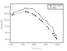
As it’s shown in Figure.7 the numerical model value is always under predicts value. Perhaps, among the reasons, is that the theoretical model takes the ambient temperature and wind speed as constant parameters in the calculation (constant inputs) on the contrary the experiment that has the fluctuation in these parameters. The solar intensity obtained experimentally is higher than the one obtained by simulation; this is due to the higher value of the Albedo that caused by the existence of the walls and a lot of equipment surround our system. The performance of FPCs for a cloudy day is shown in Figureures 8-10. The evident point is the fluctuation of the instantaneous useful energy gain (Figureure.8.b), that caused by the strong changes in solar radiations as shown in the Figureure.8.a.

Experimental and Modeling Dynamic Study of the Indirect Solar Water Heater… (Ouhammou Badr)



ISSN: 2252-8814

(a)

(b)

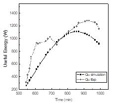
Figure 8. Solar radiations (a) and Useful energy (b) for a typical cloudy day

The retarded response is very clear in the afternoon. The useful energy and incident radiation (experimentally) has a maximum estimated about 1185 W and 1075 W/m2 respectively. The numerical model is not well estimated of the useful energy gain extracted from the system for the typical cloudy day. Also, the outlet temperature has affected in the same way by the fluctuations of the solar intensity as shown in Figure.9.

Figure 9. Variation of the outlet temperature of the working fluid for a typical cloudy day.

Nevertheless, the outlet fluid temperature of the collector was estimated with small discrepancies by simulation, i.e., the maximum experimental value is 42,8 °C when the simulation is 40 °C. It’s necessary to note that, when the solar radiations are quickly and unexpectedly increase or decrease, the fluid temperature doesn’t change immediately, and according to the changes unexpected of solar radiations, the experimental efficiency curve is very different from the simulation as illustrated in Figure.10.

IJAAS Vol. 7, No. 1, March 2018: 86 – 96

IJAAS

ISSN: 2252-8814



Figure 10. The transient efficiency of the collector for a typical cloudy day

When the solar radiation is not important, the measurements efficiency is higher than that obtained by simulation, the reason responsible for this increases value is because the difference between the inlet and outlet experimental temperatures, but for the simulation, as previously mentioned, the parameters inputs are constants. In the middle of the day, when the solar intensity increase as shown in Figure.10, the efficiency curve drops completely in a different way from that solar radiation. The reasons for those deviations between our model and experimental results as illustrate in previous Figureures are the following: a. Weather conditions, which were unstable during the experiences. b. The simulation uses all parameters as a constant input. c. The fluctuation in the measurements. d. The distance between collector and storage tank is far. e. The effect of the thermal inertia, i.e. it’s impossible to achieve initial temperatures very close to the modeled ones. f. The thermal and optic losses during the experience represent 11 % and 20-- % respectively, for example for the cloudy day , the incident energy is 16920 KJ , the losses are 1862 KJ and 3384 KJ respectively , for the sunny day the energy incident is 23400 KJ ,the losses are 4680 KJ and 2574 KJ. The measuring equipment may not be as accurate as it should be or as indicated by their manufacturers, i.e. the measurements of the solar radiation are carried out with a relative error of 10 % and 3 % for the other different temperatures sensor.

5. CONCLUSION The objective of this study was to model an indirect solar water heater with forced circulation and validate the model through simple experimental. The simulation is used on this model was shown to agree well with the experimental results such as: a. The percentage error of outlet water temperature is 2 % for the sunny days and 5 % for the cloudy days. b. The percentage error of useful energy is 4 % and 9 % for the sunny and cloudy days respectively. c. The thermal efficiency curve of FPCs follows the same shape of EN12975 standard, which the coefficients a1 and a2 are equal to those of FPCs (type SOL 200) and the percentage error between them is 1,2 %. This means that the model developed in the current work can be represented the real system and can be used to estimate its dynamic behavior.

REFERENCES [1] [2] [3]

Kalogirou SA (2004) “Solar thermal collectors and applications” Progress in Energy and Combustion Science 30:231–295. doi: 10.1016/j.pecs.2004.02.001 Duffie JA, Beckman WA, Worek WM (1994) “Solar engineering of thermal processes”, 2nd ed. Journal of Solar Energy Engineering 116:67. doi: 10.1115/1.2930068 Close DJ (1967) “A design approach for solar processes” Solar Energy 11:112–122. doi: 10.1016/0038092x(67)90051-5

Experimental and Modeling Dynamic Study of the Indirect Solar Water Heater… (Ouhammou Badr)

96 [4] [5] [6] [7] [8] [9]

[10] [11] [12] [13]

[14] [15] [16] [17] [18] [19]

[20]



ISSN: 2252-8814

Wijeysundera NE (1978) “Comparison of transient heat transfer models for flat plate collectors” Solar Energy 21:517–521. doi: 10.1016/0038-092x(78)90077-4 Kamminga W (1985) “The approximate temperatures within a flat-plate solar collector under transient conditions” International Journal of Heat and Mass Transfer 28:433–440. doi: 10.1016/0017-9310(85)90076-6 Isakson P (1995) “Solar collector model for testing and simulation” Final Report for BFR Project No. 900280-1, Building Services Engineering. Royal Institute of Technology, Stockholm. de Ron AJ (1980) “Dynamic modelling and verification of a flat-plate solar collector” Solar Energy 24:117–128. doi: 10.1016/0038-092x(80)90386-2 Huang BJ, Wang SB (1994) “Identification of solar collector dynamics using physical model-based approach” Journal of Dynamic Systems, Measurement, and Control 116:755. doi: 10.1115/1.2899275 Schnieders J (1997) “Comparison of the energy yield predictions of stationary and dynamic solar collector models and the models’ accuracy in the description of a vacuum tube collector” Solar Energy 61:179–190. doi: 10.1016/s0038-092x(97)00036-4 Achard G, Plantier C, Fraisse G (2003) “Development and experimental validation of a detailed flat-plate solar collector mode” 5th French and European TRNSYS User Meeting. France Cadafalch J (2009) “A detailed numerical model for flat-plate solar thermal devices” Solar Energy 83:2157–2164. doi: 10.1016/j.solener.2009.08.013 Villar NM, López JMC, Muñoz FD, et al. (2009) “Numerical 3-D heat flux simulations on flat plate solar collector” Solar Energy 83:1086–1092. doi: 10.1016/j.solener.2009.01.014 copyright (1994) Test methods for solar collectors -- part 1: Thermal performance of glazed liquid heating collectors including pressure drop. http://www.iso.org/iso/catalogue_detail.htm?csnumber=17678. Accessed 7 Jan 2017 Huang BJ, Hsieh SW (1990) “An automation of collector testing and modification of ANSI/ASHRAE 93-1986 standard” Journal of Solar Energy Engineering 112:257. doi: 10.1115/1.2929932 Shaner WW, Duff WS (1979) “Solar thermal electric power systems: Comparison of line-focus collectors” Solar Energy 22:49–61. doi: 10.1016/0038-092x(79)90059-8 Perrinde Brichambaut C, Vauge C (1982) Le Gisement solaire: Évaluation de la ressource énergétique [Merzouk NK, Merzouk M (2014) “Performances théoriques et expérimentales des capteurs solaires” Editions universitaires européennes Cooper PI (1969) “The absorption of radiation in solar stills” Solar Energy 12:333–346. doi: 10.1016/0038092x(69)90047-4 UNESCO documents and publications. http://unesdoc.unesco.org/ulis/cgi-bin/ulis.pl?database=ged&req=2&look=all&no=123413(accessed December 19, 2016). Accessed 7 Jan 2017 Kumar A, Unny TE (1977) “Application of Runge-Kutta method for the solution of non-linear partial differential equations” Applied Mathematical Modelling 1:199–204. doi: 10.1016/0307-904x(77)90006-3

IJAAS Vol. 7, No. 1, March 2018: 86 – 96

Institute of Advanced Engineering and Science Indonesia

: D2, Griya Ngoto Asri, Bangunharjo, Sewon, Yogyakarta 55187, Indonesia

Malaysia

: 51 Jalan TU 17, Taman Tasik Utama, 75450 Malacca, Malaysia

COPYRIGHT TRANSFER FORM (Please compile this form, sign and send by e-mail) Please complete and sign this form and send it back to us with the final version of your manuscript. It is required to obtain a written confirmation from authors in order to acquire copyrights for papers published in the International Journal of Advances in Applied

Sciences (IJAAS) Full Name and Title Organisation Address and postal code City Country Telephone/Fax E-mail Paper Title Authors

Copyright Transfer Statement The copyright to this article is transferred to Institute of Advanced Engineering and Science (IAES) if and when the article is accepted for publication. The undersigned hereby transfers any and all rights in and to the paper including without limitation all copyrights to IAES. The undersigned hereby represents and warrants that the paper is original and that he/she is the author of the paper, except for material that is clearly identified as to its original source, with permission notices from the copyright owners where required. The undersigned represents that he/she has the power and authority to make and execute this assignment. We declare that: 1. This paper has not been published in the same form elsewhere. 2. It will not be submitted anywhere else for publication prior to acceptance/rejection by this Journal. 3. A copyright permission is obtained for materials published elsewhere and which require this permission for reproduction. Furthermore, I/We hereby transfer the unlimited rights of publication of the above mentioned paper in whole to IAES. The copyright transfer covers the exclusive right to reproduce and distribute the article, including reprints, translations, photographic reproductions, microform, electronic form (offline, online) or any other reproductions of similar nature. The corresponding author signs for and accepts responsibility for releasing this material on behalf of any and all co-authors. This agreement is to be signed by at least one of the authors who have obtained the assent of the co-author(s) where applicable. After submission of this agreement signed by the corresponding author, changes of authorship or in the order of the authors listed will not be accepted.

Retained Rights/Terms and Conditions 1. 2.

Authors retain all proprietary rights in any process, procedure, or article of manufacture described in the Work. Authors may reproduce or authorize others to reproduce the Work or derivative works for the author’s personal use or for company use, provided that the source and the IAES copyright notice are indicated, the copies are not used in any way that implies IAES endorsement of a product or service of any employer, and the copies themselves are not offered for sale. Although authors are permitted to re-use all or portions of the Work in other works, this does not include granting third-party requests for reprinting, republishing, or other types of re-use.

Yours Sincerely,

Corresponding Author‘s Full Name and Signature Date: ……./……./…………

IAES Journals, http://iaescore.com/journals International Journal of Advances in Applied Sciences (IJAAS), email: iaes.editor@gmail.com, editor@iaesjournal.com

Guide for Authors International Journal of Advances in Applied Sciences (IJAAS) is a peer-reviewed and open access journal dedicated to publish significant research findings in the field of applied and theoretical sciences. The journal is designed to serve researchers, developers, professionals, graduate students and others interested in state-ofthe art research activities in applied science areas, which cover topics including: chemistry, physics, materials, nanoscience and nanotechnology, mathematics, statistics, geology and earth sciences. Papers are invited from anywhere in the world, and so authors are asked to ensure that sufficient context is provided for all readers to appreciate their contribution.

The Types of papers The Types of papers we publish. The types of papers that may be considered for inclusion are: 1) Original research; 2) Short communications and; 3) Review papers, which include meta-analysis and systematic review

How to submit your manuscript All manuscripts should be submitted online at http://iaescore.com/journals/index.php/IJAAS

General Guidelines 1) Use the IJAAS guide (http://iaescore.com/journals/ourfiles/IJAAS_guideforauthors_2019.docx) as template. 2) Ensure that each new paragraph is clearly indicated. Present tables and figure legends on separate pages at the end of the manuscript. 3) Number all pages consecutively. Manuscripts should also be spellchecked by the facility available in most good word-processing packages. 4) Extensive use of italics and emboldening within the text should be avoided. 5) Papers should be clear, precise and logical and should not normally exceed 3,000 words. 6) The Abstract should be informative and completely self-explanatory, provide a clear statement of the problem, the proposed approach or solution, and point out major findings and conclusions. The Abstract should be 150 to 250 words in length. The abstract should be written in the past tense. 7) The keyword list provides the opportunity to add keywords, used by the indexing and abstracting services, in addition to those already present in the title. Judicious use of keywords may increase the ease with which interested parties can locate our article. 8) The Introduction should provide a clear background, a clear statement of the problem, the relevant literature on the subject, the proposed approach or solution, and the new value of research which it is innovation. It should be understandable to colleagues from a broad range of scientific disciplines. 9) Explaining research chronological, including research design and research procedure. The description of the course of research should be supported references, so the explanation can be accepted scientifically. 10) Tables and Figures are presented center. 11) In the results and discussion section should be explained the results and at the same time is given the comprehensive discussion. 12) A good conclusion should provide a statement that what is expected, as stated in the "Introduction" section can ultimately result in "Results and Discussion" section, so there is compatibility. Moreover, it can also be added the prospect of the development of research results and application prospects of further studies into the next (based on the results and discussion). 13) References should be cited in text by numbering system (in Vancouver style), [1], [2] and so on. Only references cited in text should be listed at the end of the paper. One author should be designated as corresponding author and provide the following information: • E-mail address • Full postal address • Telephone and fax numbers Please note that any papers which fail to meet our requirements will be returned to the author for amendment. Only papers which are submitted in the correct style will be considered by the Editors.

International Journal of Advances in Applied Sciences (IJAAS) Institute of Advanced Engineering and Science (IAES) e-mail: ijaas@iaesjournal.com

IJAAS Journal Order Form Volume

Number

Amount

Price (Rp)

Price (USD)

Total

Name

Company

Address

City / State

Zip

Telephone/Fax

: ........................, ..........................

Signature: ..................................

Order form for subscription should be sent to the editorial office by fax or email

Payment by Bank Transfer Bank Account name (please be exact)/Beneficiary: LINA HANDAYANI Bank Name: CIMB NIAGA Bank Branch Office: Kusumanegara City: Yogyakarta Country :Indonesia Bank Account # : 5080104447117 Bank Swift : BNIAIDJAXXX >>> Please find the appropriate price in the price list on next page >>>

The price list for domestic and foreign subscribers

Volume

Number

Year

1 1 1 1 2 2 2 2 3 3 3 3 4 4 4 4 5 5 5 5 6 6 6 6 7 7 7 7 8 8 8 8

1 2 3 4 1 2 3 4 1 2 3 4 1 2 3 4 1 2 3 4 1 2 3 4 1 2 3 4 1 2 3 4

2012 2012 2012 2012 2013 2013 2013 2013 2014 2014 2014 2014 2015 2015 2015 2015 2016 2016 2016 2016 2017 2017 2017 2017 2018 2018 2018 2018 2019 2019 2019 2019

Price (IDR) for domestic subscribers 290.000,00 290.000,00 290.000,00 290.000,00 290.000,00 290.000,00 290.000,00 290.000,00 319.000,00 319.000,00 319.000,00 319.000,00 319.000,00 319.000,00 319.000,00 319.000,00 349.000,00 349.000,00 349.000,00 349.000,00 349.000,00 349.000,00 349.000,00 349.000,00 349.000,00 349.000,00 349.000,00 349.000,00 349.000,00 349.000,00 349.000,00 349.000,00

Price (USD) for foreign subscribers 36 36 36 36 36 36 36 36 40 40 40 40 40 40 40 40 44 44 44 44 44 44 44 44 44 44 44 44 44 44 44 44

The price included the printing, handling, packaging and postal delivery fees of the hardcopy to the address of the authors or subscribers (with Registered Mail). For foreign subscribers, an additional fee is charged if you would your order is mailed via Express Mail Service (EMS): - $25 for ASIA Continent - $35 for AUSTRALIA Continent - $35 for AFRICA Continent - $39 for AMERICA Continent - $39 for EUROPE Continent (No additional fee for delivering your order by Registered Mail).

International Journal of Advances in Applied Sciences (IJAAS) Volume 7, issue 1, Mar. 2018

Articles inside

Kavita Kavita, Neera Batra, Rishi Pal Singh

Anuja Das, Biswajit Mohanty, Benudhar Sahu

B. Rampriya

Samarth Borkar, Sanjiv V. Bonde

Anagha Bhunje, Swati Ahirrao

Arvind Sahu, Swati Ahirrao

Aakanksha Jumle, Swati Ahirrao

Ahmad Abdul Qadir Alrababah

Prabhu Kavin B, Ganapathy S

Yasin Yousif Al-Alaboosi, Jenan Abdulkhalq Al-Aboosi