


THE ILLUSION OF CONTROL
Aarav 7J
THE HISTORY AND IMPACT OF ZERO IN MATHEMATICS
Advait 9M1
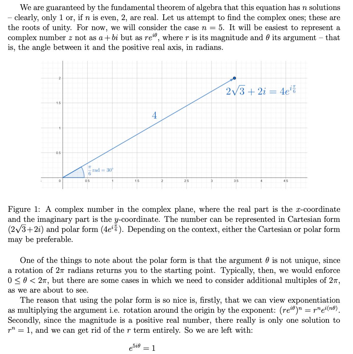
ROOTS OF UNITY
Oliver L6M2
I S S U E 3 W I N T E R 2 0 2 4

THE ILLUSION OF CONTROL
Aarav 7J
THE HISTORY AND IMPACT OF ZERO IN MATHEMATICS
Advait 9M1
ROOTS OF UNITY
Oliver L6M2
Dear everyone,
The third edition of Sigma, the HABS Maths Magazine, is here and I'm thrilled to share it with you!
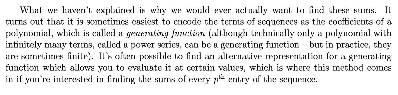
Building on the success of our last edition, we've got a whole new lineup of articles covering a diverse range of maths topics, including some familiar faces returning from the previous edition and some fantastic contributions from new writers, including Chaos theory, roots of unity, and the maths behind gambling and betting systems!
A big thanks must go to everyone who submitted articles. The effort and perseverance put together to write such articles must be commended highly.
Most importantly, we hope you have fun reading these selected articles! Enjoy!
Best wishes,
Page 3 The History and impact of Zero on Mathematics
Page 6 The Mathematics behind RSA Encryption
Page 10 The Illusion of Control: Why You Can’t Beat the Odds with Betting Systems
Page 13 An introduction to chaos theory and its role in turbulence
Page 19 What is the sum of all natural numbers?
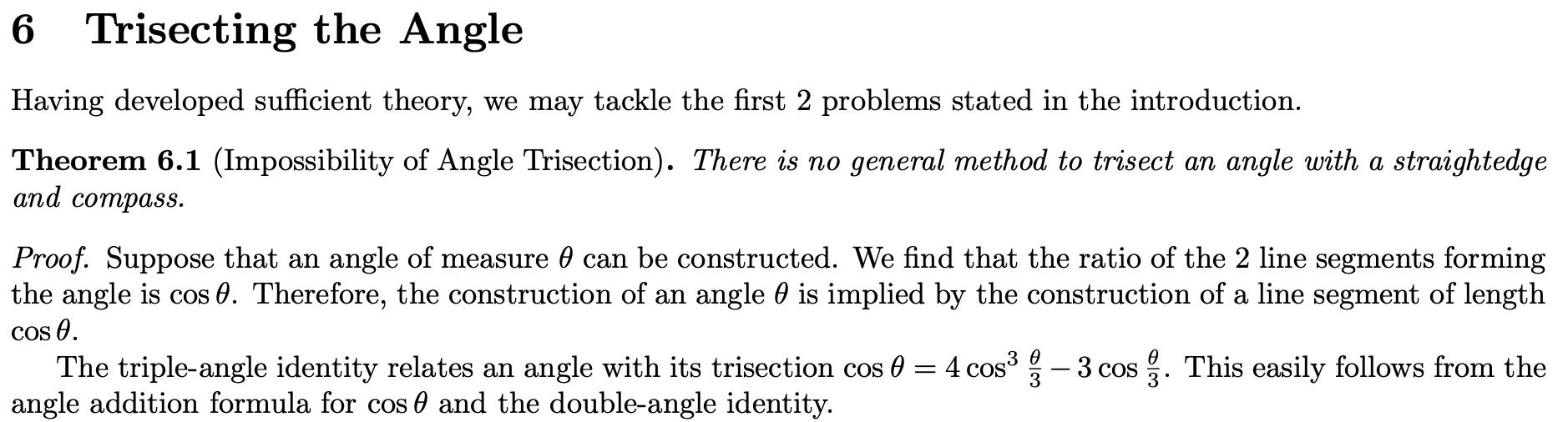
Page 24 Applications of Galois Theory to Classical Problems of Geometry
Page 30 Roots of unity: the most beautiful maths objects ever
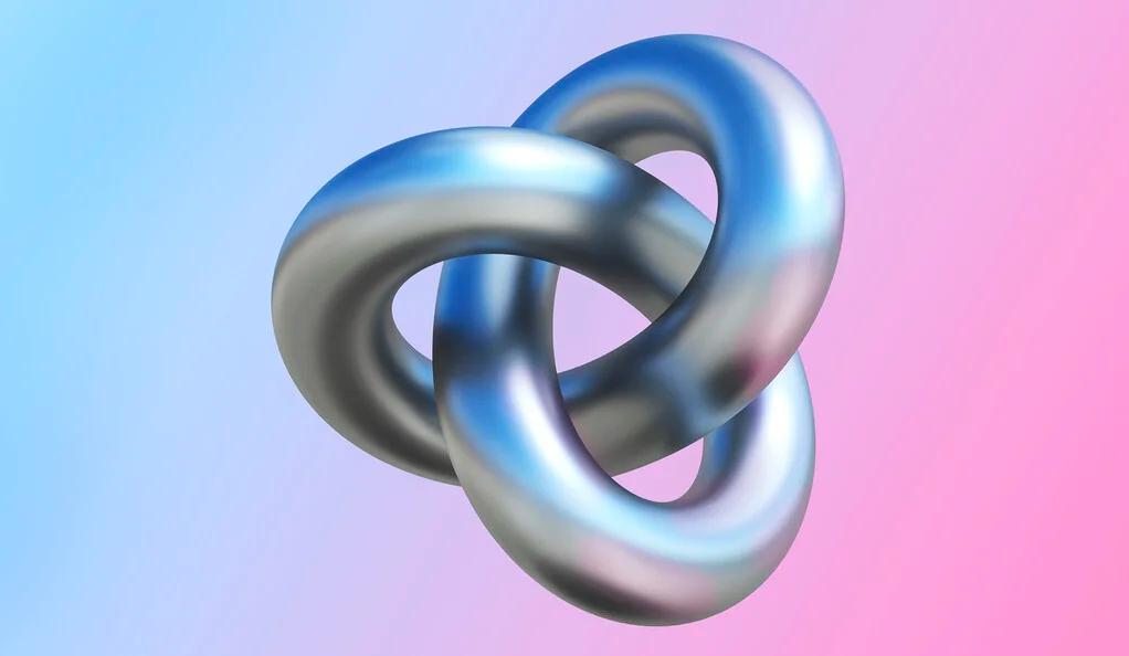
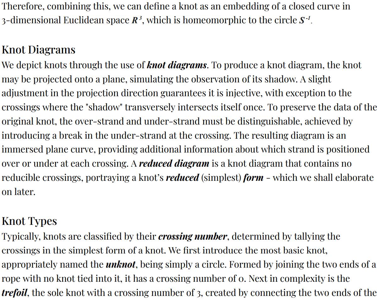
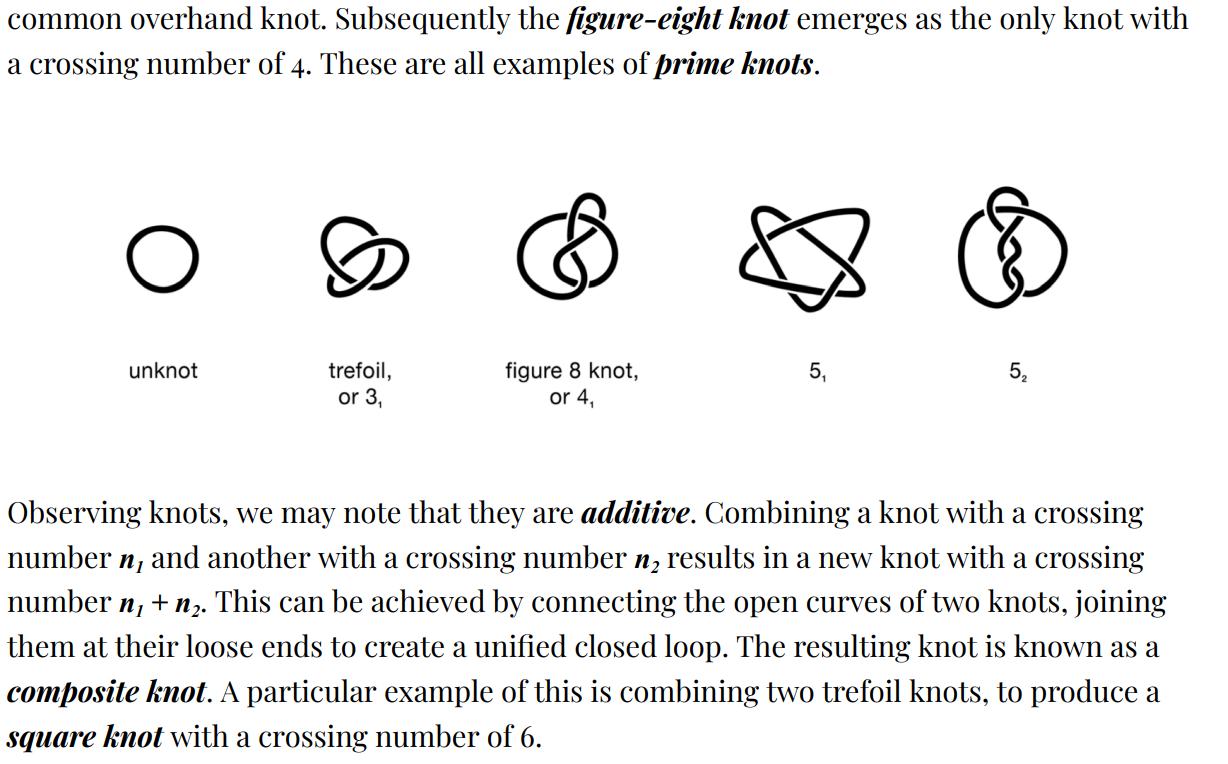
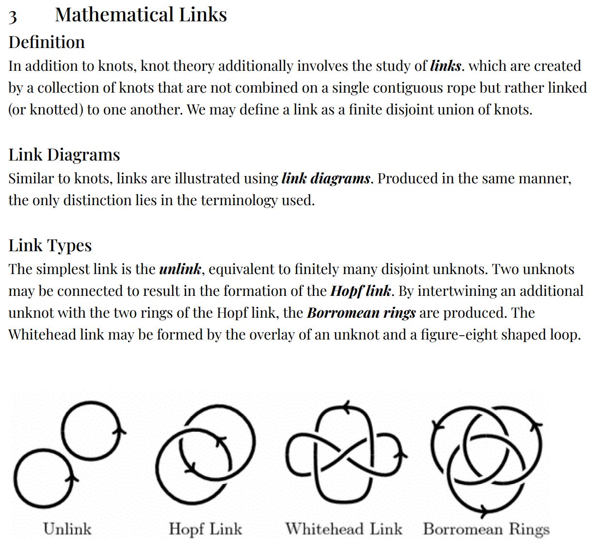
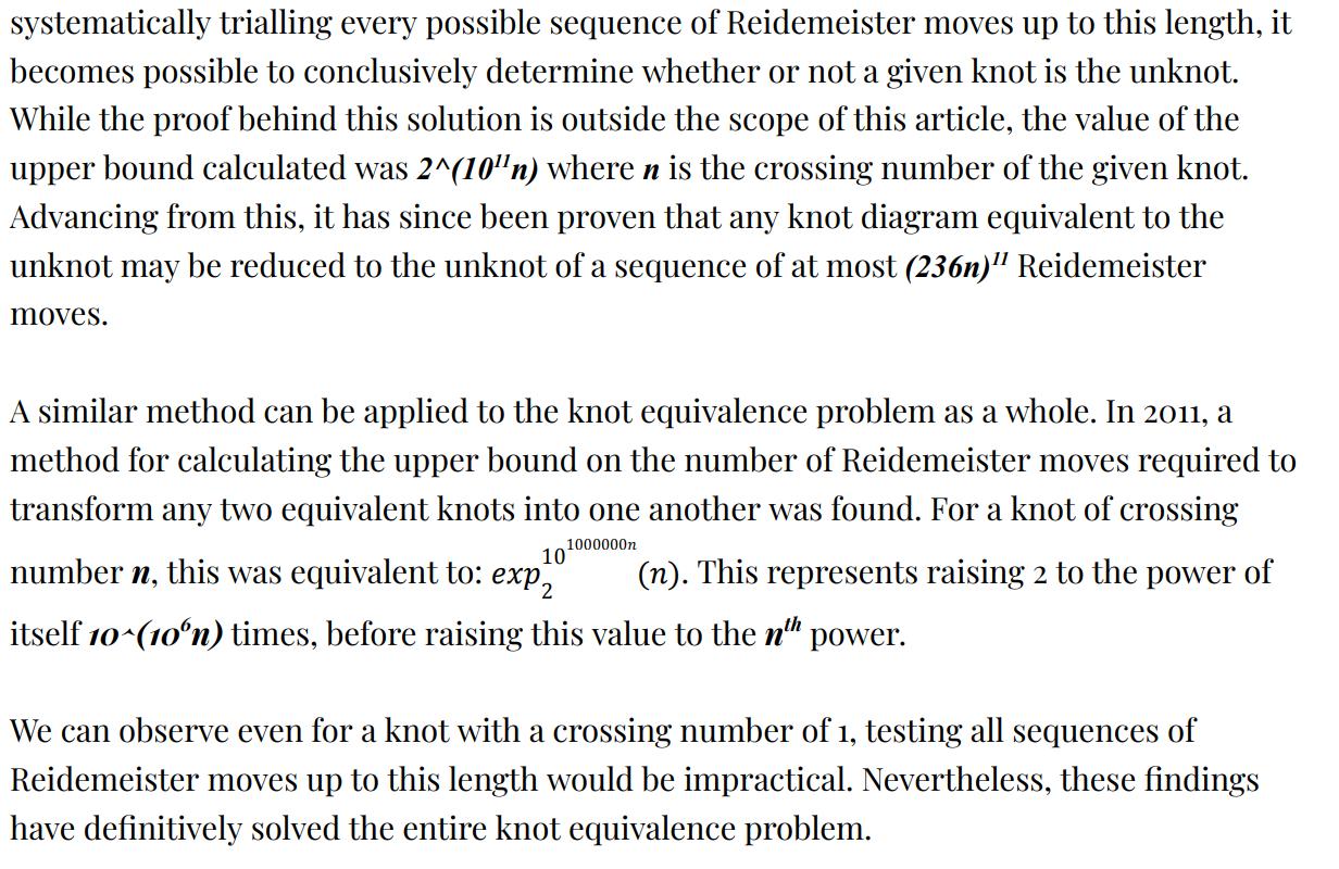
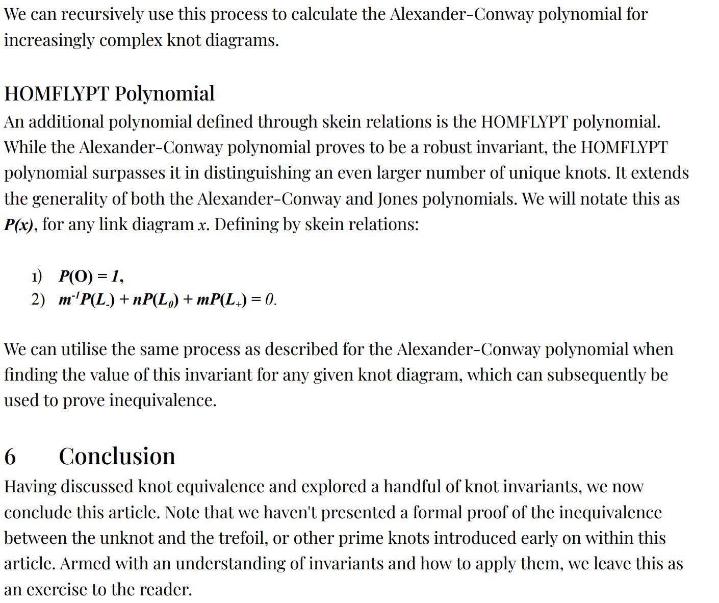
Page 38 An introduction to knot theory and the Knot Equivalence problem

Zero, an inconspicuous digit to the normal person stands at the base of our numerical understanding, creating the foundations and shaping maths as we know it. The historical journey of zero travels through ancient civilisations, accentuating the evolution of numeracy and mathematical thought. This concept of zero emerged from diverse cultures, from the great minds of ancient Indian mathematicians to the sophisticated mathematicians of Babylon As a placeholder zero’s role has transformed to be used in advanced arithmetic operations and further into modern life with binary and Computers.
This essay embarks on the journey of the number zero’s profound history and impact on mathematics as we know it From its inception to its use in the most complex of algebraic equations and calculus. Instead of just being a numerical entity, zero has been a catalyst for innovation, not just in the mathematical field. We will delve into the intricate web of the significance of zero, unravelling the threads of algebra, calculus, and computer science Beyond the world of numbers zero makes us think philosophically Join me on this
journey, tracing the footsteps of zero, uncovering its remarkable journey
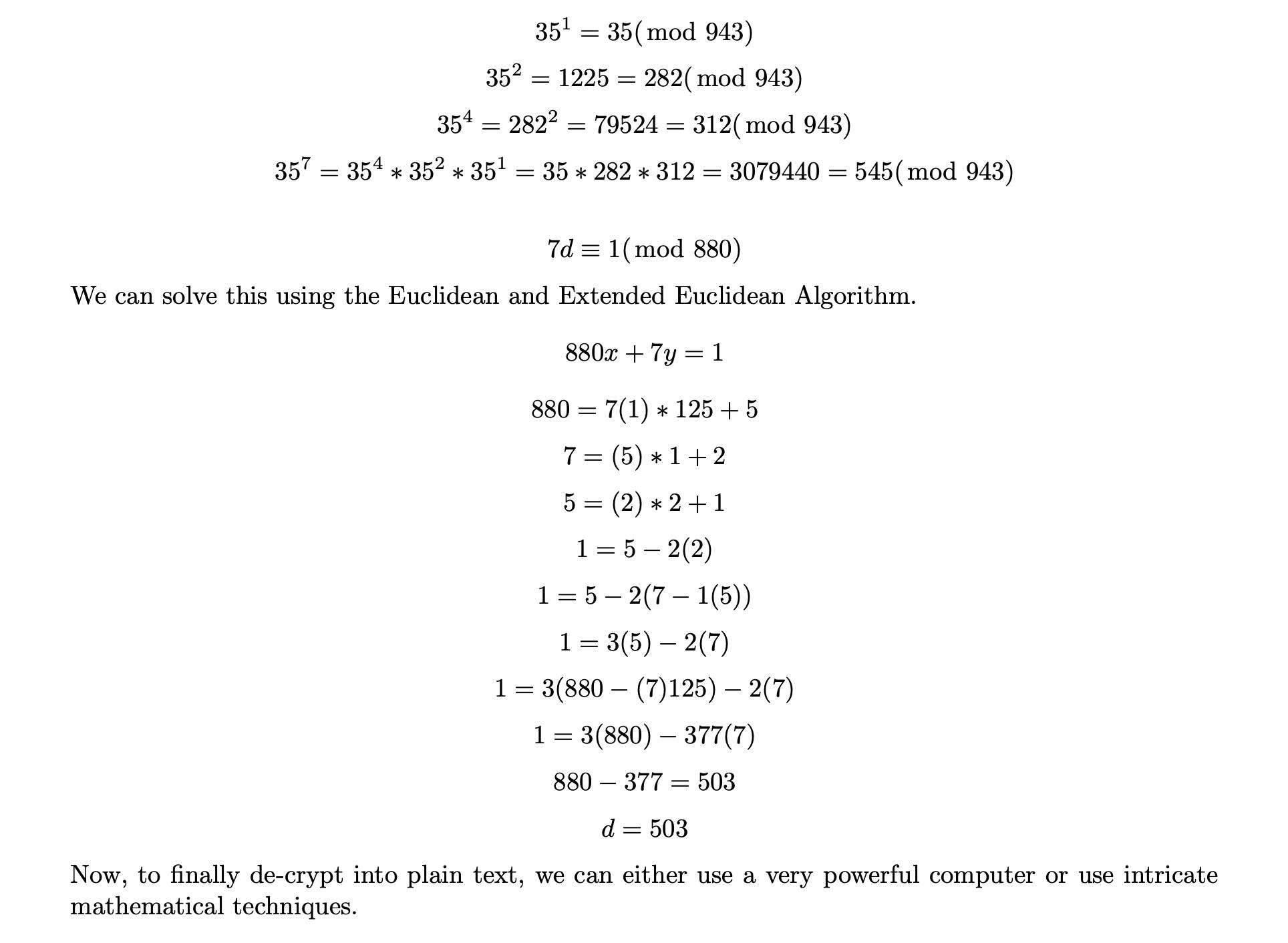
The number zero has profound roots in history, the journey that started in ancient India moved worldwide through trade. The whole concept of zero is believed to have started in Hindu culture around the 5th century CE. The word for zero in Sanskrit, the language spoken at the time in India, is śūnya, this means nothingness Mathematician and Astronomer Aryabhata is commonly known for inventing the number zero. Brahmagupta was the driving force behind zeros growth, he realised that it could not just be used as a placeholder for nothing, yet it could also be used in calculations After him, the next step on this illustrious journey of zero is Persia The 9th century mathematician al Khwarizmi is referred to as the father of algebra and is primarily responsible for spreading the concept of zero towards the Mediterranean. Fibonacci, a name known by numerous mathematicians, is the next on this list Fibonacci learnt about zero and the decimal system from Arab traders while accompanying his father on merchant tours. He realised how the decimal system was an improvement on the commonly used Roman numeric system of the time. Through his book Liber Abaci (which means book of calculation) which was published in 1202, this new method of mathematics spread throughout Europe Due to controversy, it took two millennia for the mathematical brilliance of zero to finally be accepted into society.
Zero is a placeholder, just like in the ancient days where ancient mathematicians used zero to show the absence of a number, we do this when writing numbers such as 101 or 2055 Nowadays zero is so useful we could not live without it, however, there once was a time where zero was surrounded by so much controversy that people did not want to live with it. In the year of 1299 in Florence, Italy, alongside all Arabic numerals, the number zero was banned People believed zero could be used fraudulently, it could be doctored into a nine and shopkeepers could add a few extra zeros to the receipt to blatantly inflate the price. Zero was seen as dangerous as it was the gateway to negative numbers, with negative numbers representing debt It took so much time that finally in the 15th century zero was accepted
In Algebra zero plays a pivotal role by being both a placeholder and a critical element used in equations. When zero is incorporated into expressions it serves as
a crucial point of reference. Zero in itself, allows mathematicians to denote the absence of a quantity Zero has a key role in establishing the concept of inverses and it forms the basis for subtraction and division. In manipulations, zero acts as a pivot for addition and subtraction. Zero is the piece of the algebraic puzzle which keeps everything in place. It allows us to figure out where things balance or cancel out Zero makes equations simpler and solvable
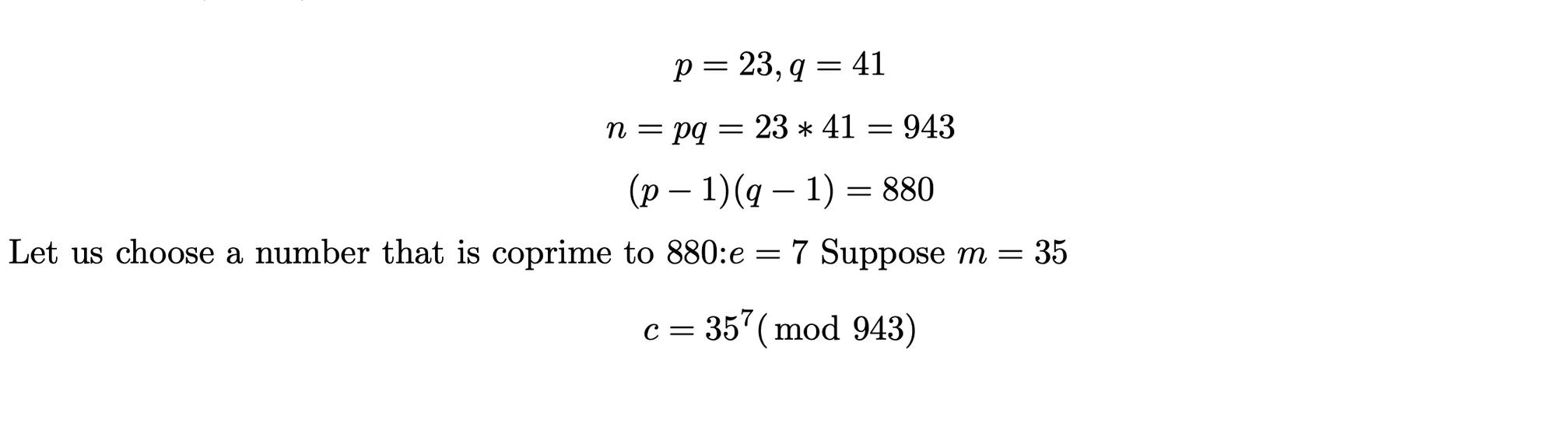
For some mathematicians Euler’s identity is the most beautiful equation as it comprises of the five most important mathematical constants. People compare this equation with the likes of Shakespear’s Sonnets Physicist Richard Feynman claims that it is ‘The most remarkable formula in mathematics.’ Of course, this equation includes the number zero. Euler’s identity is written as: e^(iπ) + 1 = 0. The 5 most important mathematical constants in this equation are: Pi, the number one, the imaginary number i, the number e, and zero In this equation, zero plays the profound role of uniting the five fundamental constants. Zero, here, acts as the equilibrium point creating harmony between the imaginary and real components. Zero here truly highlights the beauty of mathematics and how unrelated elements can bond into an excellent equation
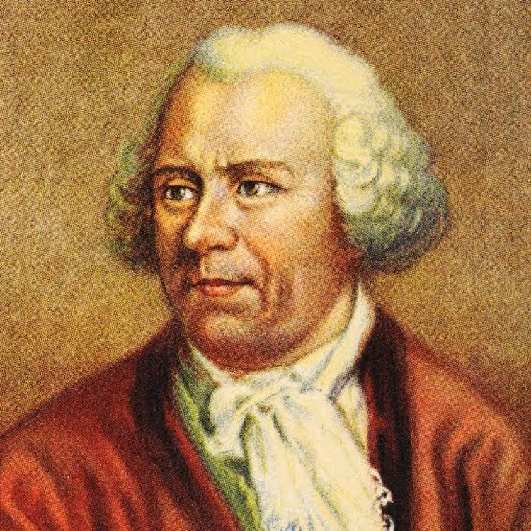 Figure 2: (Leonhard Euler, responsible for creating Euler's identity)
Figure 1: (Brahmagupta, an instrumental figure in the development of zero)
Figure 2: (Leonhard Euler, responsible for creating Euler's identity)
Figure 1: (Brahmagupta, an instrumental figure in the development of zero)
Apart from the complex fields of maths, zero plays a pivotal role in computer programming, mainly in the context of binary representation In the binary system, which is the fundamental language of computers, information is displayed simply using two digits, zero and one This code forms the basis of all digital data In binary representation, zero represents no signal whereas one indicates a signals presence. The interplay of zeroes and ones allows computers to execute complex calculations and store loads of data and information. Through binary encoding the data is transformed into various patterns of zeros and ones allowing for representation of text, numbers, and other various forms of multimedia. Thanks to the binary system computers can perform intricate operations quickly and regularly Without zero’s inclusion in binary framework, the remarkable capabilities of computers and modern technology would not be achieved today
In philosophy, zero and infinity can evoke philosophical reflections. Zero represents absence and a void which is high in contrast to infinity’s boundlessness. Yet zero can also be seen as a starting point, a blank canvas from which mathematicians can develop as they have done over the years and infinity suggesting the unending possibilities. This intertwines with calculus where zero and infinity are the limits, demonstrating the divergence
Zero’s journey through history is a truly epic tale, evolving from a placeholder to a pivotal thread in the web of mathematics. Its historical significance is deeply rooted in its gradual change from an abstract concept to a symbol which is tangible. Zero is truly indispensable, shaping not only the foundations of modern-day mathematics but also practical applications to assist us in our understanding of the vast universe of numbers. In the intricate tapestry of mathematics, our existence is inseparable from the mysterious presence of the number zero Our mathematical systems, from simple and basic arithmetic to the most complex algebra or calculus, rely upon the fundamental job performed by zero. Zero serves as the nexus for numerical operations, whilst also being pivotal in day-to-day appliances and applications. Our technological presence right now is a testament to zero. Essentially, we navigate our numerical world thanks to the irreplaceable role zero plays in the fabric of our mathematical reality.

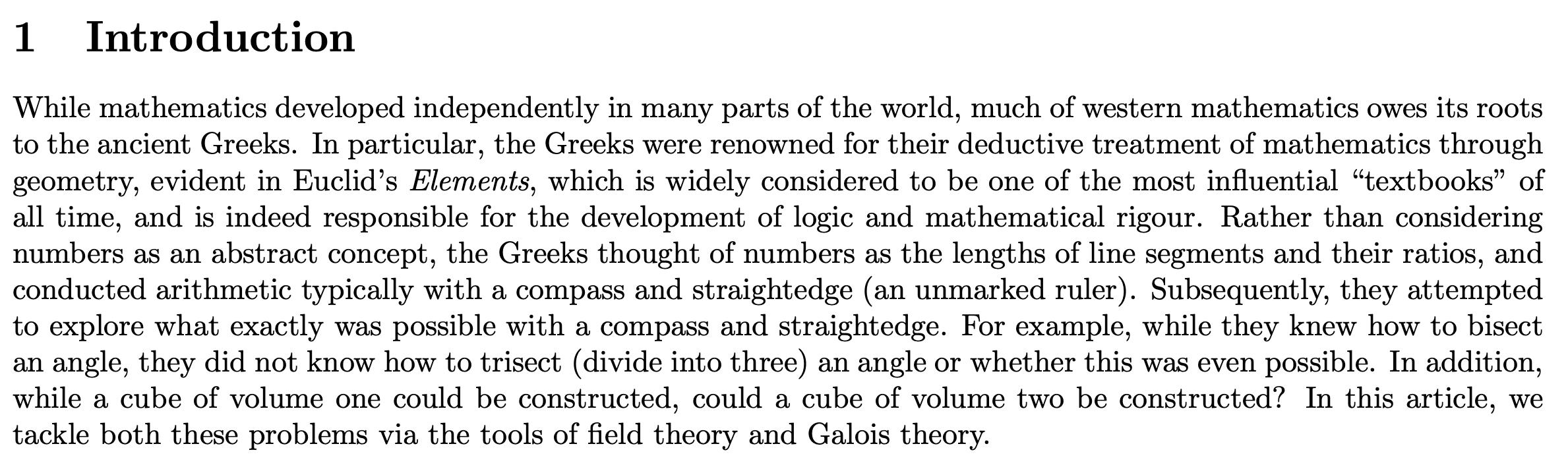
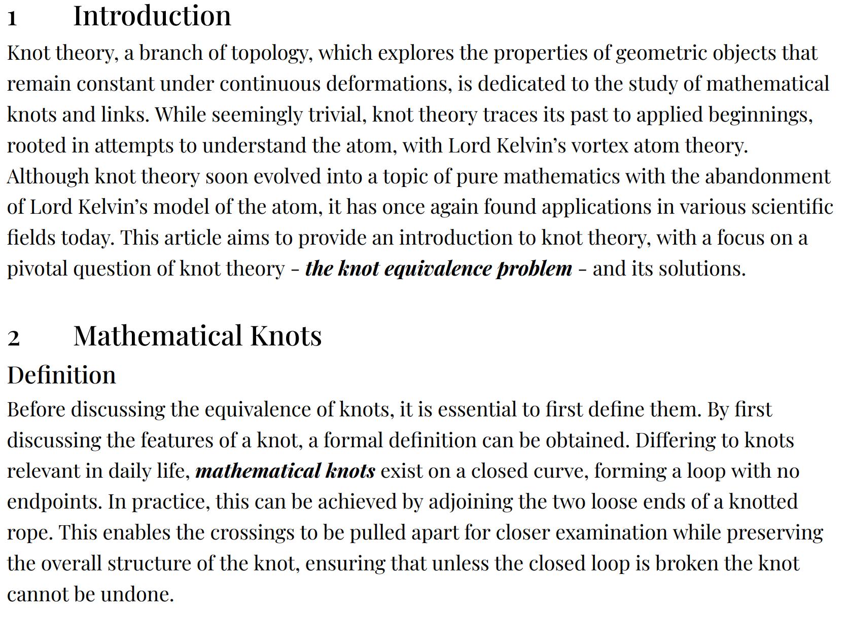
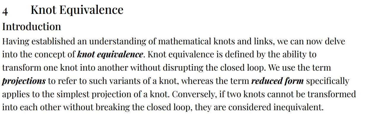
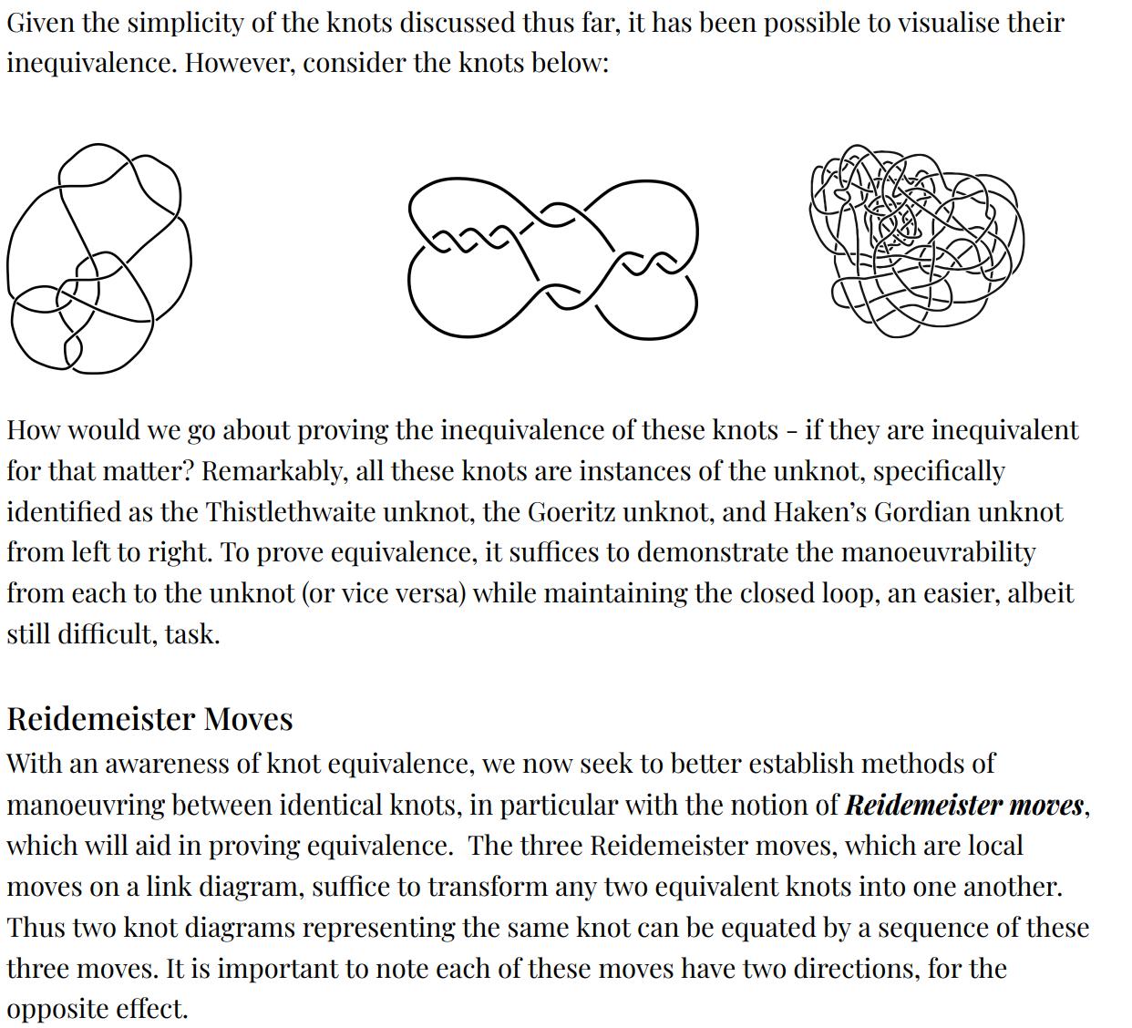
Introduction
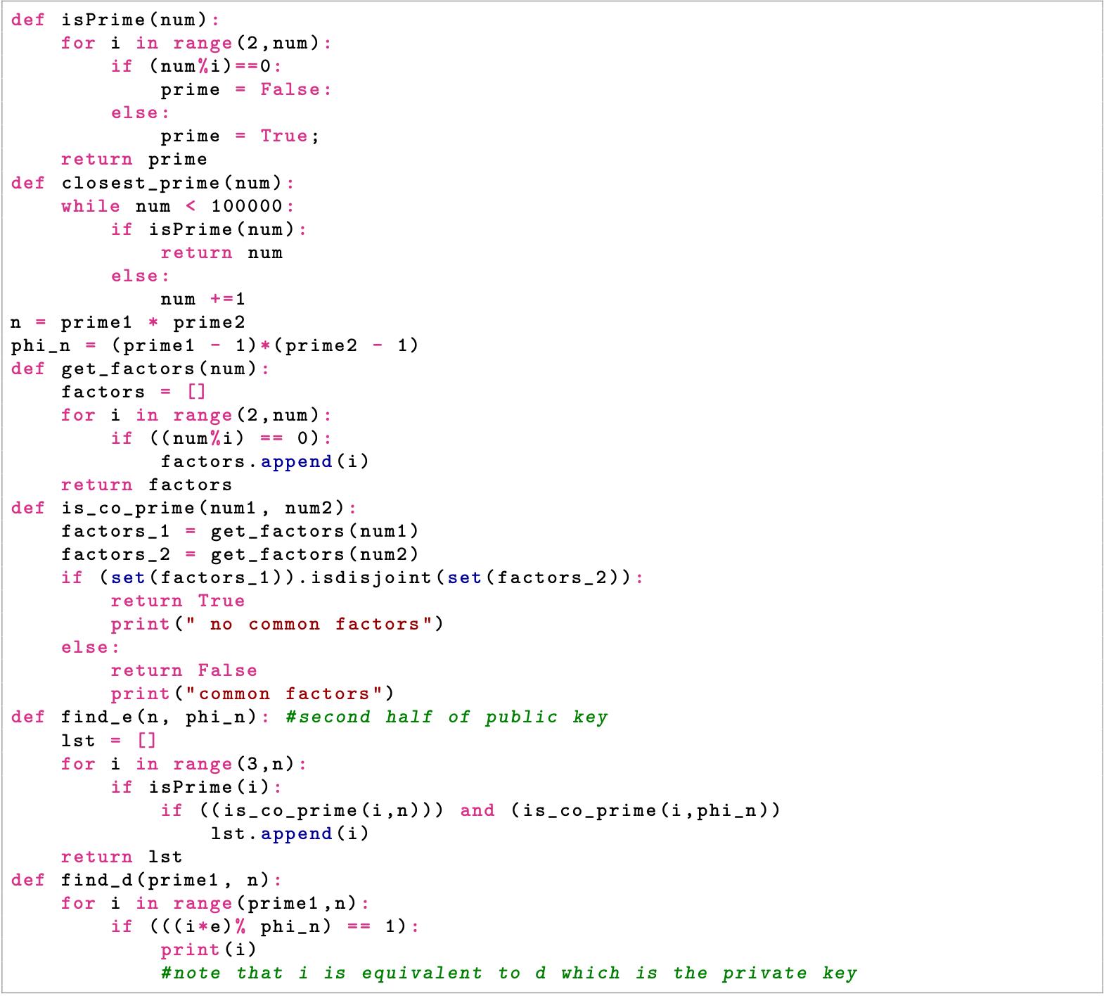
RSA encryption algorithm, also known as Rivest-ShamirAdleman encryption algorithm is used widely in cryptography as an assymetric algorithm. An assymetric algorithm uses two keys, public and private where the public key is able to encrypt any data sent by the sender and the private key is the key that is able to decrypt the data sent to them but is only available to the receiver to prevent any eavesdropping This article will explore the use of number theory in the encryption process, disadvantages and advantages as well as possible solutions to overcome the encryption.
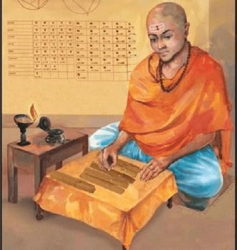
It is imperative to note that the algorithm is based on the fact that multiplying two large numbers is easy but factorising a large number is much more difficult. Firstly, the receiver i.e the person wanting to send data chooses two large prime numbers, namely p and q. Let their product n = pq be the first half of the public key To remind us, this key is what will encrypt the data After, we then use the Euler’s Totient function denoted by ϕ(n). The Totient function counts the number of positive integers less than n that are also coprime to n. m ∈ N such that 1 ≤ m < n and gcd(m, n) = 1. Say we have ϕ(7), then numbers, 1, 2, 3, 4, 5, 6 will be listed where m is relatively prime to n so therefore ϕ(7) = 6 The receiver calculates that ϕ(pq) = (p 1)(q 1) We know this because firstly, we list integers, p, 2p, 3p, ....(q 1)p that have a common factor with n. Therefore, another list, q, 2q, 3q...(p 1)q also have a common factor with n so these must be eliminated from the n 1 positive integers that are less than n.
The first list has q 1 exceptions and the second list has p 1 exceptions and therefore n 1 (p 1) (q 1) = pq p q + 1 = (p 1)(q 1) positive integers that are less than but also relatively prime to n We have now proven this: ϕ(pq) = (p 1)(q 1) so the next step is choosing a number e which is relatively prime to ϕ(pq) and this will be the second half of the public key. Let us denote m as the plain text Using c ≡ m^e (mod n) we can then get the encrypted message as denoted by c What will be told to the sender is n and e c can be formed with those two values and m, the plain text. The receiver also solves this equation, de ≡ 1(modϕ(n)) where d is the private key.
1 2 Process
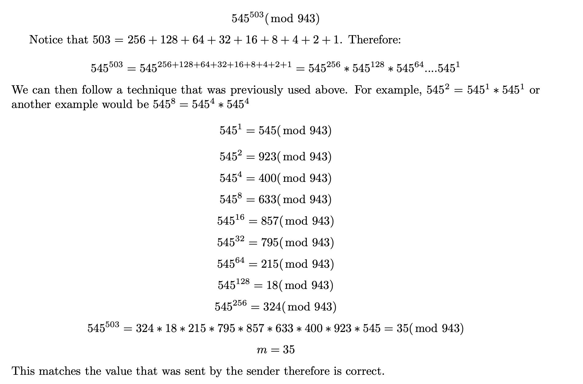
To quickly summarise, the sender is able to use the ASCII table to map his letters into numbers and then using c ≡ m^e (mod n), we get the encrypted message, c otherwise known as ciphertext. Then, using c^d ≡ m(mod n), we can get the number, m which can then be unwrapped back to its original letter Another approach can be as follows: de ≡ 1(mod (p 1)(q 1)) where e is the second half of the public key and p, q are unique prime numbers. Solving the equation to get d and plugging into equation c^d (mod n) ≡ m where m is plain text. Let us calculate this with actual values (pasted on other side, PTO):
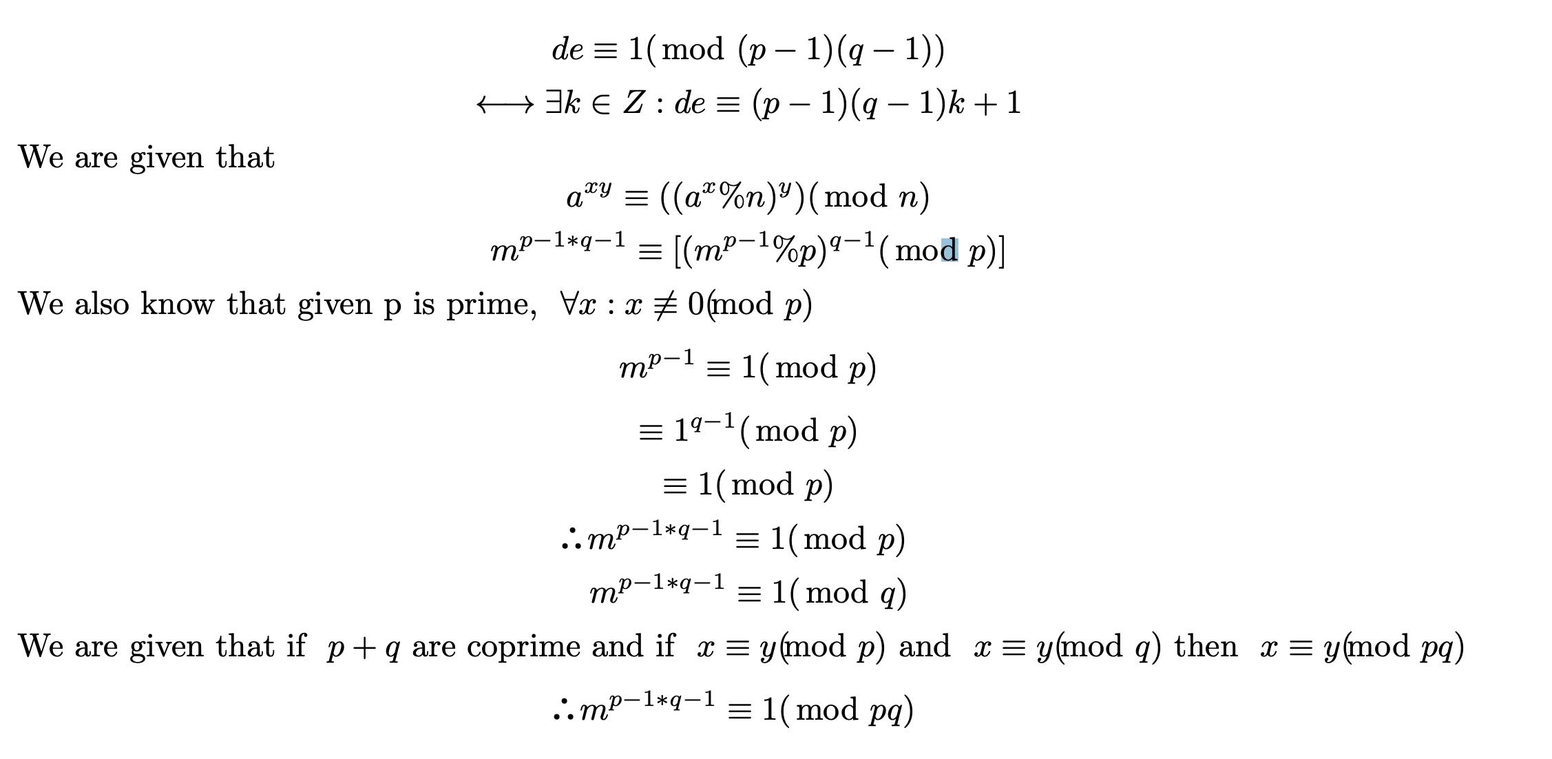
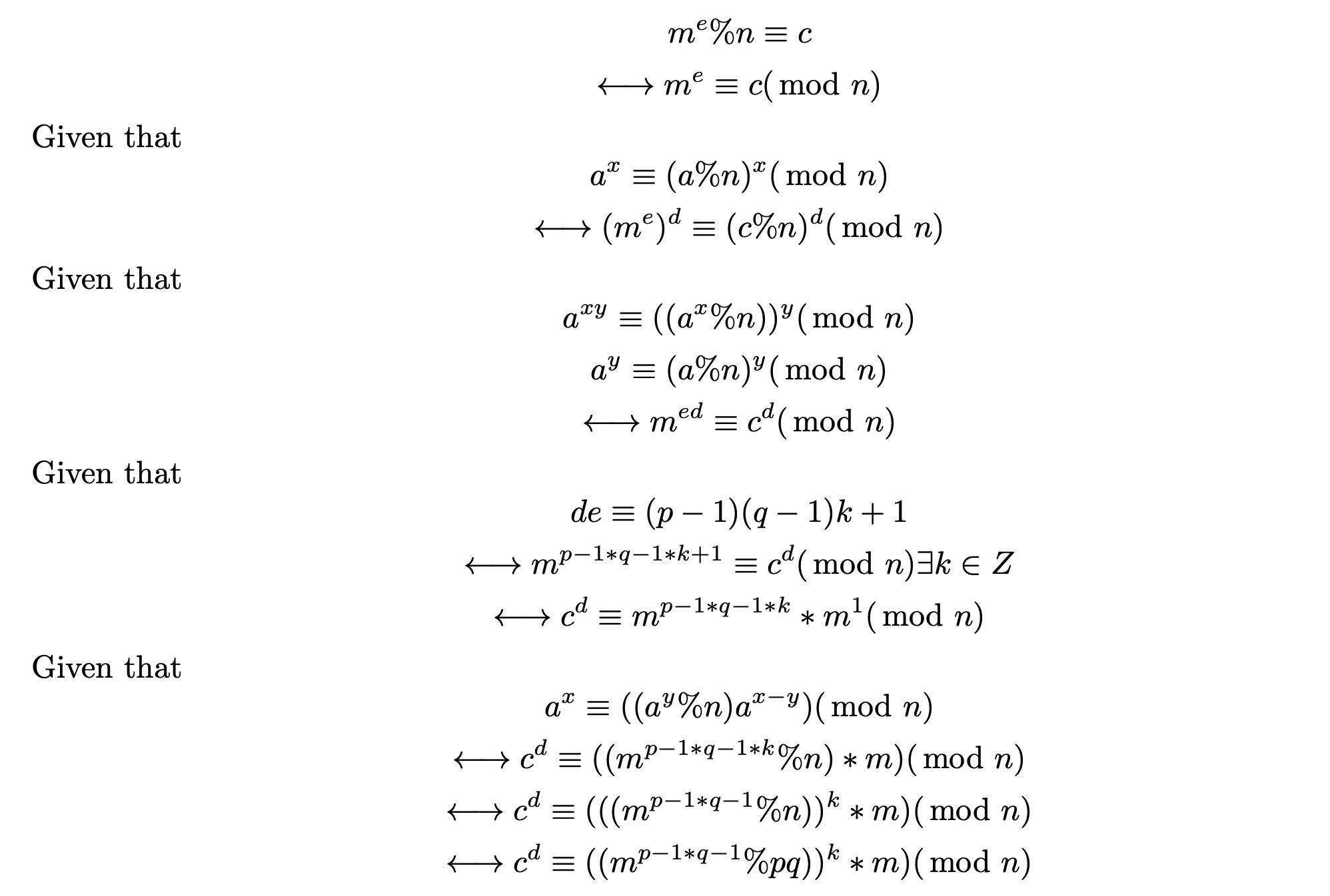
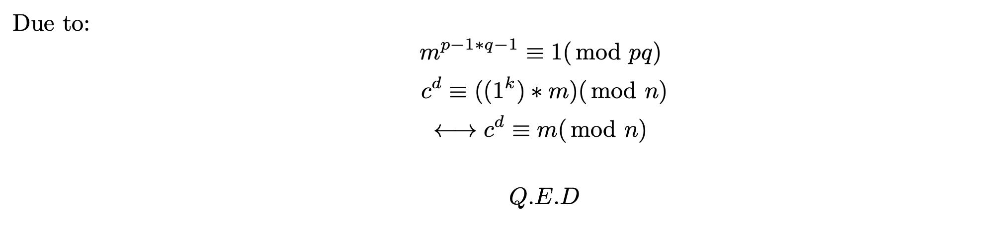
Firstly, we are proving this statement Let us remind ourselves of the symbols again for convenience Plain text, encrypted message, first half of public key and second half of public key, first prime number and second prime number are denoted by m, c, n, e, p and q. If m^e %n ≡ c is true and n = pq and p + q are prime and de ≡ 1(mod ϕ) where ϕ = (p 1)(q 1) and 1 < e < ϕ and e and ϕ are co-prime then c^d %m) ≡ n is true.
There are numerous advantages and disadvantages
The advantages are seemingly obvious but vital to consider for one point is that there is no means to exchange a secret key, otherwise known as the private key. It is also easy to implement mathematically and because of the fact that it involves very large numbers, it is very hard to decrypt the cipher text back into plain text. However, in the modern era that is to come, we see that an algorithm known as the Euclidean algorithm, that of which was used above, can compute the greatest common divisor of two numbers and if the GCD ≠ 1, then the public keys can be broken simultaneously Also, if m^e < n then the private key can easily be determined Another important disadvantage would be the use of quantum computers which use algorithms that are able to factor numbers at a faster complexity than other hardware. In particular, an algorithm named Shor’s would be used in the quantum computer.
RSA is a widely used and known algorithm seen throughout many applications, some of which may be used be all of us Examples include digital signatures, secure communication protocols like HTTPS and SSH, software protection, email encryption, as well as online banking.
Since the concept of gambling strategies was first thought of, players have always sought ways to beat the odds In this article, I will discuss common betting strategies that people employ, the maths behind them, and big issues with them.
The Martingale strategy is a strategy used in a game of roulette (This can only be used in a game where your money is doubled when you win) and dictates that every time you lose your bet, you should double it on your next bet. However, if you win your bet, you should go back to the amount you betted before losing anything.
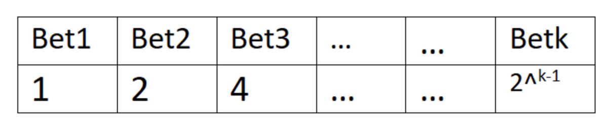
We can spot a pattern in the amount of money we have to bet every time we lose, which is 2^k-1. For example, if we are on bet number 5, we would have to bet 2^ (5-1) or 16 pounds.
Now imagine that we are on bet number k, and we lose This means that by using the formula for the sum of a geometric series and our previous knowledge we can find that we have so far lost 2^k - 1. As our next bet is bet number k + 1, if we win, we will gain 2^k on it which will lead to an overall profit of one pound Therefore, whenever we win, we will end up covering all previous losses and winning one pound
This sounds quite good, but there are a few problems with this strategy.
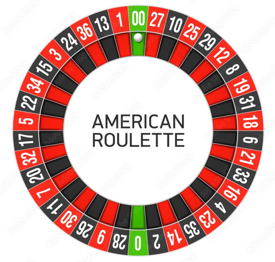
For example, casinos know about this strategy too and that is why the green 0 and 00 on the roulette table and maximum bet limits stop you from having a good chance of winning
Even if these rules were not in place, there are still problems with the Martingale strategy. For example, this strategy only gets you money for sure if you have unlimited money. As a player would only have a finite amount of money, which I will call N here, it is possible to lose money This can happen if the amount you need to bet on your next turn (2^k) is greater than N.
Take the boundary case where 2^k = N. The probability we lose k times is 1 / 2^k or 1/N. This means the chance of losing your money is 1 divided by the amount of money you started with This means the chance you make profit is 1 – 1/N. So however high your chance of winning, it is not certain since N is finite.
Note that we assumed 2^k was equal to N which is a boundary case and because 2^k can also be greater than N, there are other cases and the probability of making profit can change
Another interesting thing is the chance of doubling your money. This probability can be calculated as (1 - 1/N)^N. As N goes to infinity, this equation reaches a limit of 1/e. Therefore, however much money you put in, you cannot get a better chance of doubling your money than 1/e or about 37% There is one exception which is if you only have one pound and try to double your money on first bet, which becomes a game with equal chances of losing all your money or doubling your one pound and so the probability is 50%.
There are many variants to this strategy, though none of them are faultless and some do not make sense at all. For example, there is a strategy in which a player is advised to only start betting after three even-chance events have happened The logic is that normally if you start with £1 and have £100 in total, after 7 consecutive losses you will be broke If you use this variant, there will have to be 10 times in a row for the ball on a roulette table to go against the colour you are betting on.
There is a big problem with this approach though This strategy assumes that previous events have an impact on future events On a roulette table, this is not true The chance of 8 same events happening does not change, whether there have been 3 of the same events before them or not.
Overall, you would be better off just betting all your money on red or black if you wanted to double your money, but the strategy and its variants are still commonly used to gain a little bit of money.
The endless quest for £100
Just like the Martingale strategy, this is about roulette and shows how there is one strategy you should definitely not implement in roulette.
Alice and Bob are players who both have an aim of making 100 pounds but having different strategies Alice has 10,000 pounds and keeps on betting 1 pound on red until she either runs out of money or makes 100 pounds from her strategy. Bob only has 100 pounds and decides to bet all his money on red immediately. Assuming there are 18 reds, 18 blacks and 2 green zeros on a roulette wheel, these are the approximate chances of them making 100 pounds
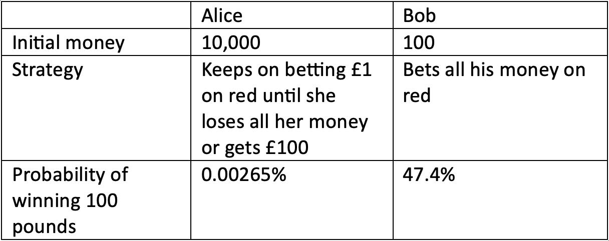
At first sight, these results are shocking How can Alice have such little chance of making 100 pounds when she starts with 10,000? It turns out that with Alice’s strategy, even someone starting with 100 trillion pounds could only have an improvement of 4 642467 * 10^-61 % from Alice’s probability This is where we can use a formula to help us realize why this happens
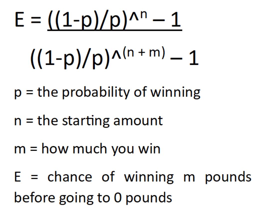
If p is not equal to ½ , then this equation will provide the results for Alice’s strategy for all values of the starting amount, the amount you want to win and the probability of winning.
When we look at the general formula, we see there is both a power of n in the numerator and the denominator which is why increasing n doesn’t make a huge effect Instead, we notice that the values of m and p make a bigger difference to the value of E
After looking at this, you can see how the strategy of betting 1 pound at a time, which seems intuitive, is a big mistake and will very rarely win money as it is a losing strategy.
This is another betting system that is used in all kinds of games which dictates that you should always bet according to the Fibonacci numbers. If you lose your bet, you should then bet the next Fibonacci number; while if you win your bet, you should go back two numbers in the sequence and bet that much
The reasoning of the system is that if you win, you are able to cover up the losses of your previous two sizes of bets This can be seen in the example in the table below
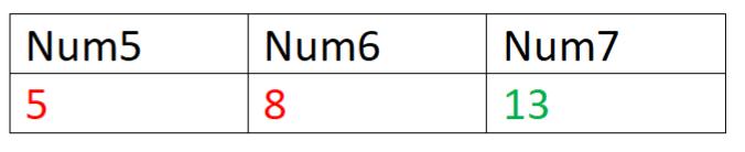
Above you can see that the successful bet of 13 covers up the previous two losses and then we move two numbers back. Therefore, each win allows us to cover the two losses before that and we hope that eventually we will be able to gain profit
This system is less risky than the Martingale strategy as we do not double our last bet and is a safer option and a way to try to avoid maximum bet limits while making money.
However, the strategy has a few unique risks which apply only to it. While it may take 15 losses to exceed a betting limit of 500, when you win with this strategy you do not go back to the smallest bet, unlike the Martingale strategy This means that it is very easy for you to lose money that you won previously as you are still betting big amounts.
Also, due to a house edge involved, the chance of losing is more than the chance of winning which severely reduces your chances of making profit overall.
Similarly, to the Martingale system, this is not a foolproof strategy and will not win much money, though the maths behind it is interesting to look at.
In conclusion, while the Martingale, Fibonacci betting systems and other methods may be popular, they are not foolproof. Maybe one day someone will find an unbeatable strategy, but until then, it is important to remember that every game in a casino is one that favours the casino, and no betting system can guarantee a win.
Introduction:
Chaos theory is the mathematical field of study which explores the unpredictability built into deterministic non-linear dynamical systems. It deals with systems that appear to be orderly (deterministic), but conceal chaotic behaviours, whilst also dealing with systems that appear to be chaotic, when, in fact, they have underlying order They are deterministic because they consist of a few differential equations, and aren’t in fact random, but are chaotic whenever its evolution depends on the initial conditions. Thus, deterministic systems are not predictable , despite knowing the initial state of the system and its governing set of equations.
Recurrent characteristics of a chaotic system include:
No periodic behaviour
1. Sensitivity to initial conditions
2. Nonlinear dynamics
3. Fractals 4 Feedback loops
5
Whilst the word Chaos, which comes from the Greek word “Khaos” (meaning ‘gaping void’) may imply randomness, it means a state of total confusion or unpredictability in the behaviour of a complex natural system, where small differences in initial conditions can produce drastically diverged outcomes for complex systems. Chaotic systems are unstable since they have many variables, with exogenous factors, such as parameters, communication with other systems and small perturbations, included as random variables This prevents us from making any long-term predictions about the system. As chaotic systems have many variables, they become highly unstable and extremely sensible to perturbations. Thus, even if we do know the initial state and the governing laws of a system, we would only be able to predict the near future state of the system, because as the chaotic system evolves from its initial state, it becomes increasingly chaotic and random
Chaotic systems are extremely common in nature, with chaotic phenomena often being described by fractal maths (never-ending complex patterns, self-similar across different scales, that are created by repeating a simple process in an ongoing feedback loop).
These phenomena can be found in rivers, clouds, trees, our hear and the brains of living organisms On a larger scale, chaotic systems can be spotted in meteorology, the solar system and fluid dynamics.
The discovery of Chaos theory:
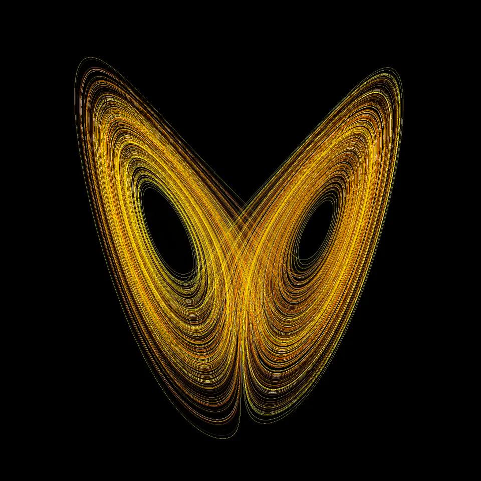
Chaos came into focus in the 1960s, when meteorologist Ed Lorenz developed a mathematical model to simulate the way air moves in the atmosphere. He had 12 equations and 12 variables such as temperature and humidity The computer would print out each time step as a row of 12 numbers, to see how the numbers would evolve over time. The breakthrough occurred when Lorenz decided to repeat a run, using a shortcut He entered the numbers from halfway through a previous printout and then set the simulation. When Lorenz saw the results he was stunned. The new run followed the old one for a short while but then it diverged, and soon it was describing an entirely different state of the atmosphere
The real reason for the difference came down to the fact that the printer was rounded to three decimal places, but the computer rounded to six. Thus, when he entered those initial conditions, the difference of less than one part in a thousand created totally different weather just a short time in the future. The tiny change in numbers led to a dramatic divergence in results, demonstrating no matter how small a deviation there is in the initial values of a simulation, the errors will accumulate rapidly, making a prediction worthless. Lorenz’s system displayed what’s become known as Sensitive Dependence on Initial Conditions (SDIC), one of the key components of a chaotic system The fact that we can never measure reality precisely enough makes it difficult to model real systems because the initial discrepancy between reality and measurements will always cause the model and reality to diverge in an unpredictable way, leaving us unable to predict what exactly will happen in the future.
The double pendulum:
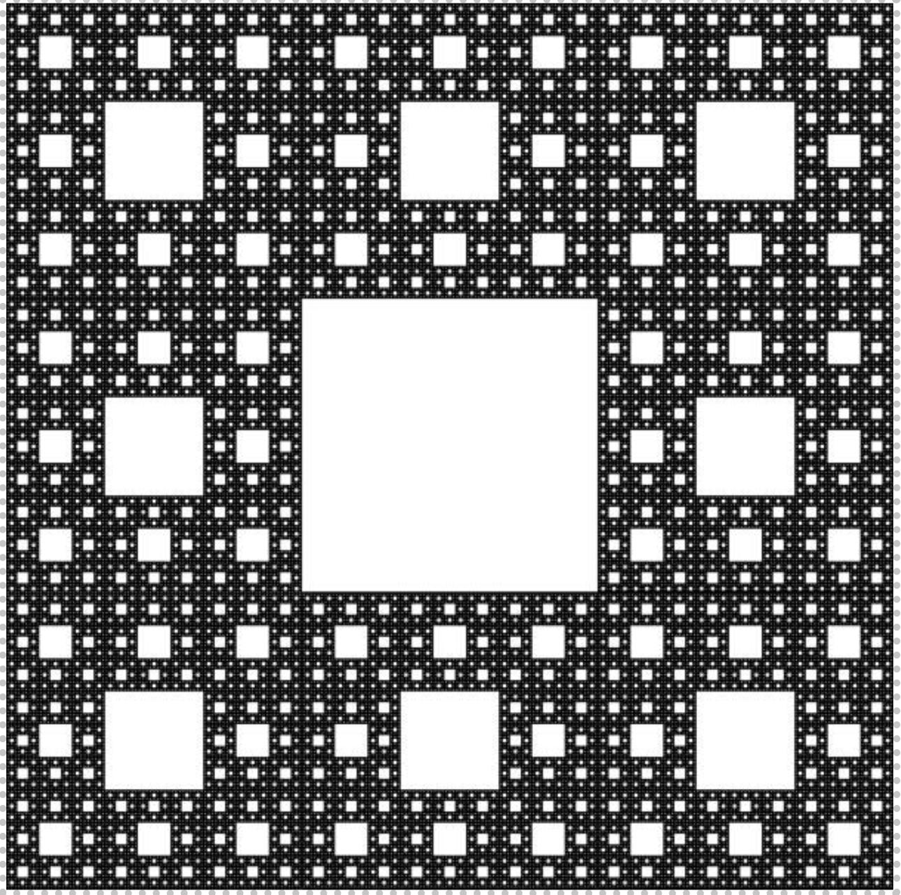
One of the simplest demonstrations of chaos theory is a double pendulum. It consists of two pendulums connected end to end. Whereas the motion of a single pendulum is predictable, it will go through an oscillatory motion and then come to equilibrium, the motion of a double pendulum is not. With the double pendulum having two degrees of freedom, for small angles the pendulum gives us simple harmonic motion, similar to the linear motion of a double spring However, when the angles are larger, the motion becomes non-linear and seems chaotic. This is shown in figure 1, where the motion of the double pendulum is seen to be much more chaotic than the motion of the pendulum in figure 2 Figure 3 also shows how the motion of the double pendulum in figure 2 is chaotic as it produces a fractal pattern.
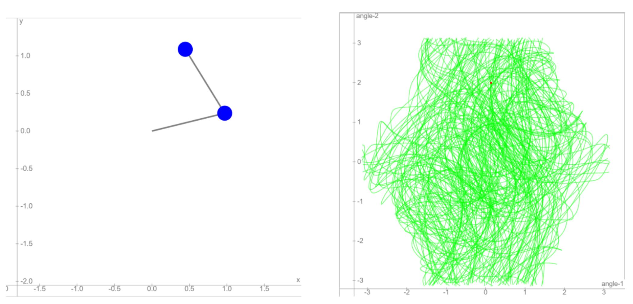
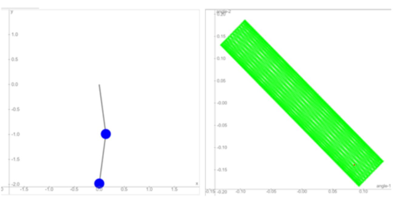
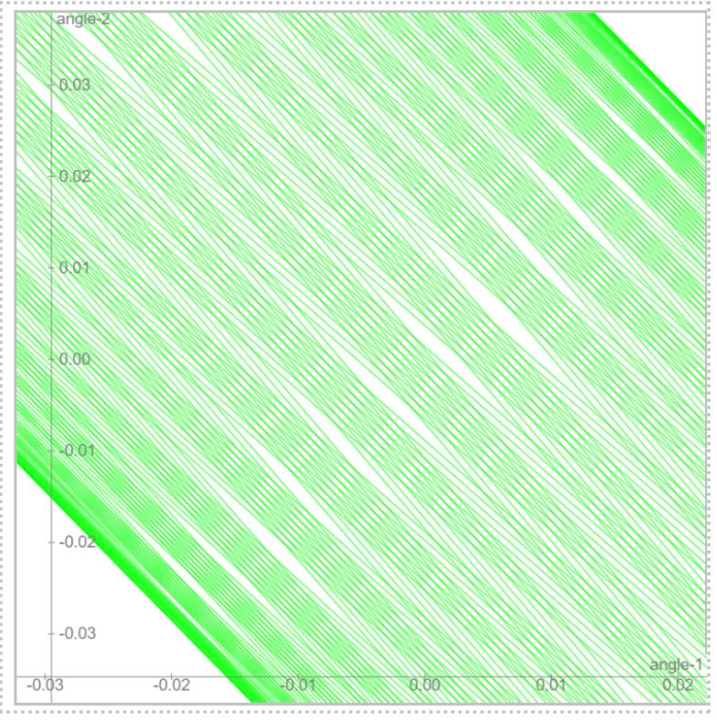
Figure 4 Zoomed in picture of the graph in figure 2, showing a fractal nature
Whilst we can describe the motion of a double pendulum using a system of differential equations, derived from the equations of acceleration and the forces acting on the pendulum, we cannot predict the motion of the pendulum by solving the equations.
The problem lies in the double pendulum system's extreme dependence on initial conditions We cannot predict the behaviour of the system if we are unable to determine the initial conditions with 100% uncertainty with absolute confidence. Since it is impossible to attain that degree of certainty, we simply cannot predict the motion of a pendulum. Even if two double pendulums were released from the same position at the same time, any arbitrarily small variation in their initial conditions will lead to drastic divergence in their trajectories in a very short period of time, with the divergence increasing exponentially, going back to Lorenz’s work on Sensitive Dependence on Initial conditions. The double pendulum
system stresses how we cannot make accurate predictions about chaotic systems
The idea that deterministic systems can exhibit seemingly random and unpredictable behaviour connects chaos theory to fluid dynamics, especially turbulent flow. Turbulent flow is a classic example of a chaotic system, with it being a nonlinear dynamical system, one of the main focuses of chaos theory. Before analysing how and why turbulence is chaotic we must first define turbulence, which is quite hard to do. Quoting Richard Feynman, turbulence is the most important unsolved problem of classical physics. It is extremely difficult to rigorously define turbulent flow and as of yet, there isn’t a universally agreed upon definition. However, there are many characteristics that we can use to determine whether a flow is turbulent.
Turbulence, in essence is unpredictable and chaotic
It is sensitively dependant on initial conditions, making it impossible to render a precise deterministic prediction of its evolution and so we can only speak about it statistically, a key attribute of chaotic systems. Whilst it is governed by the Navier-Strokes equations, they are almost impossible to solve mathematically and provide smooth solutions for any given set of initial conditions
Another characteristic of turbulence is its composition of interactive eddies (swirling fluid structures), which span a huge range of sizes. Additionally, turbulent flow is dissipative; the energy of the larger eddies cascades into smaller eddies until the eddies reach the smallest scale and dissipated their energy to the fluid as heat, affecting the viscosity of the fluid.
Turbulent flow is also diffusive. It mixes and spreads things out throughout a fluid, such as the energy and momentum of isolated parts in the fluid to the rest of the fluid. Turbulence may also include strange attractors (set of points in phase space which attracts all the trajectories in an area surrounding it, producing a fractal pattern) and fractals too, highlighting its chaotic nature.
What makes the Navier-Stokes equations chaotic?
The Navier-Stokes equations are a set of deterministic partial differential equations, relating to the velocity, pressure, temperature and density of a flowing liquid, that determine the motion of fluid They can be seen as Newton’s second law of motion but for fluids. Whilst they are not chaotic in a mathematical sense, turbulent flow (a chaotic phenomenon), arises from the Navier-Stokes equations it is governed by, particularly due to the nonlinear nature of the set of equations and their sensitivity to initial conditions.
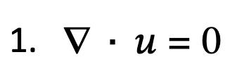
Assuming that the fluid is Newtonian, incompressible and isothermal, the first equation is the conservation of mass within the fluid, also known as the continuity equation. Here, u represent the velocity of the fluid, a vector. The operator, , is called the divergence of a vector field, in this case the velocity, , vector fluid of the fluid A fluid can not simply just disappear in an area; it may change form but its mass is conserved. Since mass is conserved, the divergence across the fluid has to be zero, and hence the first NavierStokes equation.
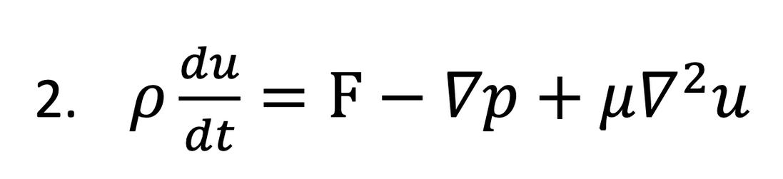
The second equation is the conservation of momentum, where u is the fluid velocity, p is the fluid pressure, �� is the fluid density, and μ is the fluid dynamic viscosity It is derived from Newtons’ Second law of ma = ΣF, where the sum of forces acting on a body is equal to its mass times acceleration.
Deriving the left side of the second equation from ma = ΣF for a single molecule of a fluid, it results in mass, m ¸ being replaced by density, with the mathematical reasoning being that to consider each individual point, we have to divide mass by volume, resulting in density, ��. Acceleration, a, is replaced with as acceleration is the derivative of the velocity To derive the right hand side of the equation, all the forces acting on a molecule of fluid need to be considered This can be broken down into internal forces and external forces acting on the molecule in the fluid. The internal force is the change in pressure from, written as the gradient of pressure The second internal force that is considered is viscosity, expressed as Finally, F denotes any external force that needs to considered, with it commonly being gravity.

Though, if the Navier-Stokes equation seems logical, how does it lead to exhibiting chaotic behaviour, such as turbulence? Once again, we are dealing with a deterministic system that is unpredictable. One reason is the coupling of velocity and pressure, creating a feedback loop that amplifies perturbations, harking back to Lorenz’s idea of Sensitive Dependence on Initial Condition The chaos in the Navier-Stokes equation also arises from the non-linear convective term of acceleration,
in the conservation of momentum equations Due to the fact that this term involves the product of two velocity vectors, its acceleration depends on the magnitude and direction of both vectors, making it nonlinear Hence any convective flow, whether turbulent or not, will involve nonlinearity However, the nonlinear convective term becomes larger as turbulent flow increases, to the point it is larger than the viscosity term, causing instability, with there being enhanced sensitivity to initial conditions, leading to the system becoming unpredictable and thus chaotic. The coupled nature of the equation and its nonlinearity consequently makes solving the Navier-Stokes equations analytically almost impossible and as a result cannot be used to predict turbulent flow
Conclusion:
The chaotic nature of the Navier-Stokes equations leads us to the question of the accuracy of Computational Fluid Dynamics (CFD). In spite of all the advances made in CFD, the "deterministic" system governed by the non-linear Navier Stokes Equations will produce unstable and unpredictable, behaviour and this lies at the heart of the difficulties with modern CFD One of the challenges lie in accurately specifying initial conditions and sensitivity in initial conditions, with the smallest variations in the data for the initial conditions causing huge divergences in the predicted results The absence of analytical solution to the Navier-Stokes equations adds to the difficulty in obtaining accurate and reliable predictions in turbulent flow scenarios. Subsequently, we are aware that CFD is still unrealistic and simplified, with the majority of differential equations utilised in the dynamical systems, that model nature, lacking solutions and, in any event, modelling the wrong thing anyway. Ultimately, these are idealised approximations are chaotic systems themselves, and are ‘solved’ on computers by the use of computational techniques that are likewise chaotic! As proposed by Professor Charles L Fefferman, the current methods may not be sufficient to fully understand and solve the challenges posed by the interplay of chaos, uncertainty and current mathematical limitations of the Navier-Strokes equations, underscoring the need for continued research and “deep new ideas” in the field of fluid dynamics.
What would happen if you were to add every single positive integer? A popular video made by the Numberphiles explores a possible answer and its ramifications are useful in even the practical branches of physics. (The answer they came to is quite surprising)
Now, the obvious answer is infinity because this sum involves a divergent series, that is a series of numbers that continually increases and therefore does not possess a finite limit. A convergent series, on the other hand, does have a finite limit and can be solved. An example of a convergent series is the sum of all inverse square numbers:
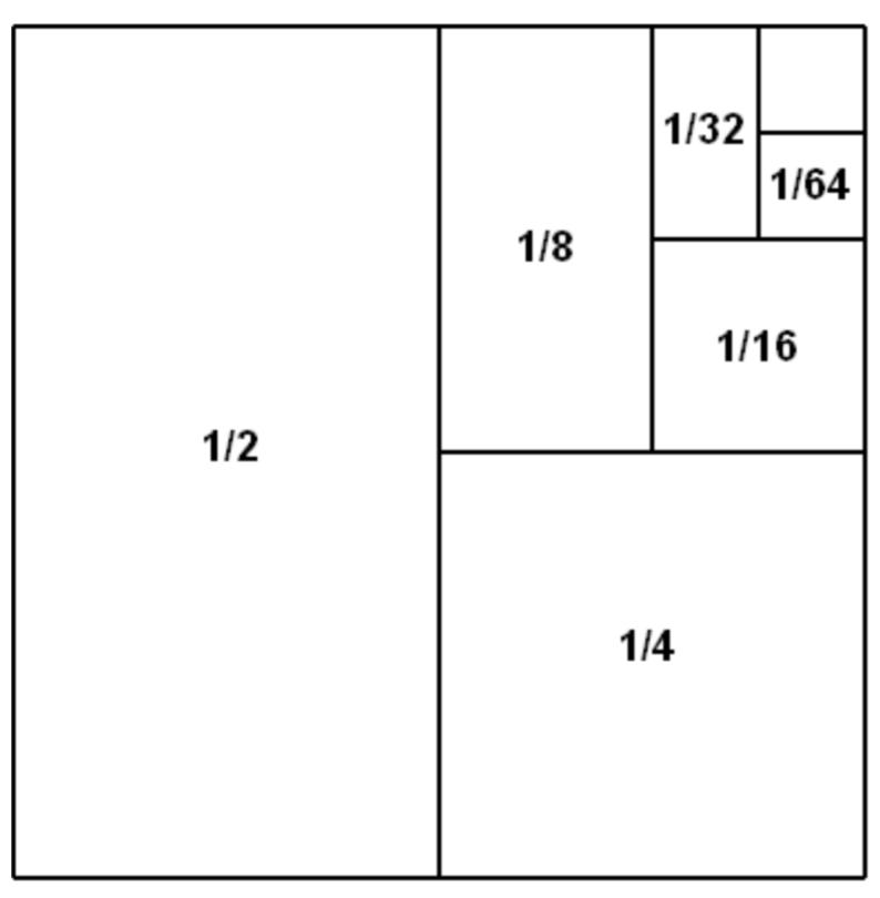
Although there are an infinite number of values in this series, its sum can be proven geometrically to converge to 1:
The numerically true solution of a divergent series is impossible to quantify by simple addition alone. If you were to add every number from 1 to however far you got by the end of the lifespan of the universe, you would have an incredibly large positive integer, but you would not have added everything to infinity and therefore, the answer could not be calculated this way. As such, mathematicians have turned to alternative methods to find a finite solution
The Ramanujan Summation was named after Srinivasa Ramanujan, who had previously explored many different infinite series. A video made by the Numberphiles Youtube channel demonstrated a method which shows that the sum of all natural numbers would be -1/12.
Their method involves splitting up the problem into various simpler infinite series.
The first of which is called Grandi’s series.
S₁= 1 1+1 1+1 1+1…= ?
This is a famous problem first proposed by the Italian philosopher Guido Grandi in 1703 Considering that this is an infinite sum which alternates between even and odd positions, there could be one of two answers depending on if you stop on an even number or an odd number. If we cut it off after 3 numbers, we get 1 1+1=1, but if we stop at 4, we get 1 1+1 1= 0
This would give an indicator that the answer would be one of these two values, but using another step, we can discern that is not the case.
If we take, 1 - S₁ , we get 1 (1 1+1 1+1 ); by flipping the signs of everything in the bracket, we get 1 1+1 1+1 1+1… which is the same as S₁ .Therefore, 1 S₁ = S₁ ⇒ 2S₁ = 1, and as such we get S₁= 1/2.
The second sum used is S₂ =1 2+3 4+5 6…
We now need to add S₂ to itself, but we need to do this in a very specific way By shifting the second S₂ one place to the right, it arranged like this:
1 2+3 4 +5 6 +7…
+ 1 2 +3 4 +5 6 which gives us: ��
Therefore, 2S₂ = 1/2 and S₂ = 1/4
Now we have all the prerequisite information and we can now solve our original Sum.
We now just need to subtract �� from S₂ 1+2+3+4+5+6+7…
[1 2+3 4+5 6+7 ] which gives us:
4 + 8 + 12 … which continues increasing in increments of 4.
If we factor out 4, we get 4(1+2+3+4+5+6+7 ), which is just 4(��).
This gives us an equation that we can use to solve for S:
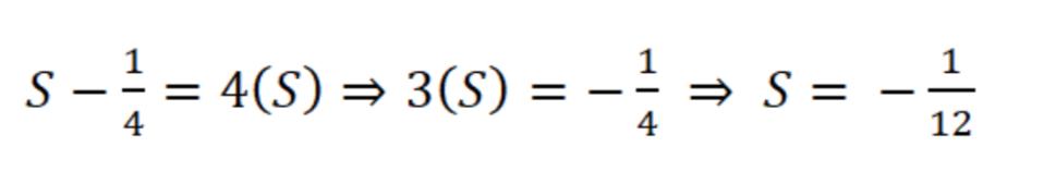
Unfortunately, there are several problems involved when dealing with infinite series, specifically with adding/subtracting them form one another and factorising them Another answer can be demonstrated by grouping this infinite series in a different way
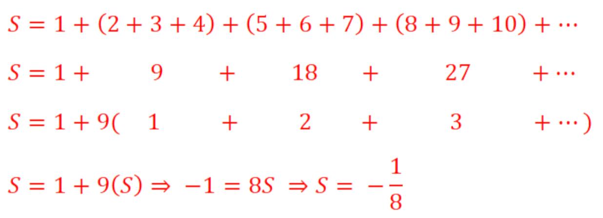
This method uses a similar approach as the Numberphile’s video and very clearly does not obtain the same answer which casts a doubt on the validity of this proof. The main problem encountered is that the rules of finite algebra (factorizing, adding brackets and even adding zeros) cannot be applied to an infinite series because of their fundamental differences Doing so, would change the entire series, changing it into an entirely different one
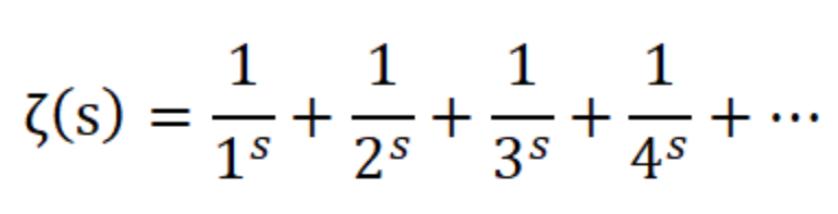
A useful function which is often referred to as the Riemann Zeta function, ζ(s). This function sums up an infinite series for the value of s.
Although the domain of the Zeta function is only defined for positive numbers, Reimann showed that it could be extended to negative numbers and even into the complex number line using a technique called analytic continuation, which Python uses to plot the negatives as well Reimann’s hypothesis states that the zeta function is equal to zero when s equals a negative even number or a complex number who’s real component is equal to two
As an aside Reimann’s hypothesis remains one of the great unsolved mysteries of mathematics. There is a prize of 1 million dollars available to anyone who can prove the hypothesis or provide an example of a zero located somewhere else
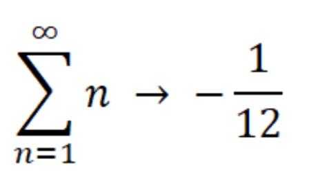
When s = -1, the Reimann zeta function becomes 1 + 2 + 3 + 4 + … which is just the sum of all natural numbers.
The python library SciP contains the zeta function, which uses this method of analytic continuation to calculate the zeta function for any value of s Python therefore is able to plot a visual representation of the Riemann Zeta function, as shown by the script below and the graph (PTO):
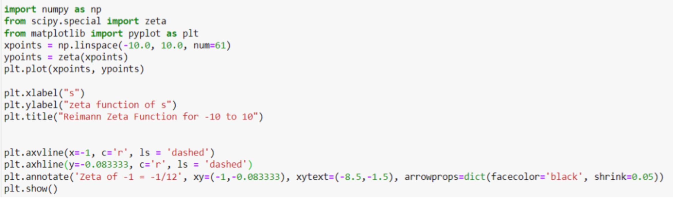
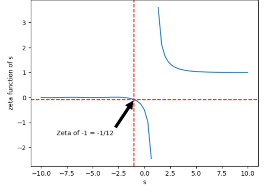
As shown on the graph, when s = -1, the Reimann Zeta function appears to cross the point - 0.8333, which is -1/12.
Although the result is questionable at best, this conclusion is immensely important in the realm of string theory and in quantum physics to such a degree that some calculations would be impossible without -1/12 being correct.
An example of this is present in calculations in quantum physics that requires infinite sums However, if we input the value of the Ramanujan Summation as infinity, we get answers that do not work and have no real functionality, whereas if we use -1/12, we can achieve realistic, useable answers, no matter how absurd it may seem.
As well as that, in string theory, if we do take -1/12 to be the correct value, it necessitates the exitance of 26 dimensions in our universe, which is quite a leap from the 3 we are familiar with
The result of -1/12 has also been used to mathematically explain the Casimir effect; the Casimir effect being the mysterious force that would cause two mirrors within a vacuum to attract one another This is thought to be brought about because of quantum fluctuations in the vacuum which create a tiny but finite force. This requires us to compute every potential wavenumber which we can accomplish by replacing the sum of all potential wavenumbers with -1/12 and using quantum mechanics, physicists have mathematically explained this phenomenon.
Overall, the only sensible solution to the sum of all natural numbers is infinity however, we have seen that -1/12 has been useful in providing a finite solution to solve real world problems by avoiding infinities in maths. Although the Numberphile video may have been criticised for lacking mathematical rigour, they were successful in exploring an interesting take on infinite series as well as providing a somewhat plausible reason as to why -1/12 works.
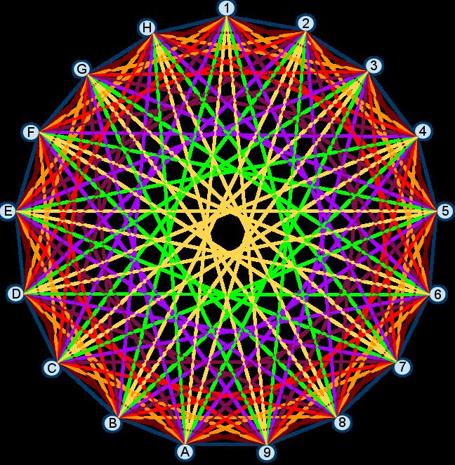
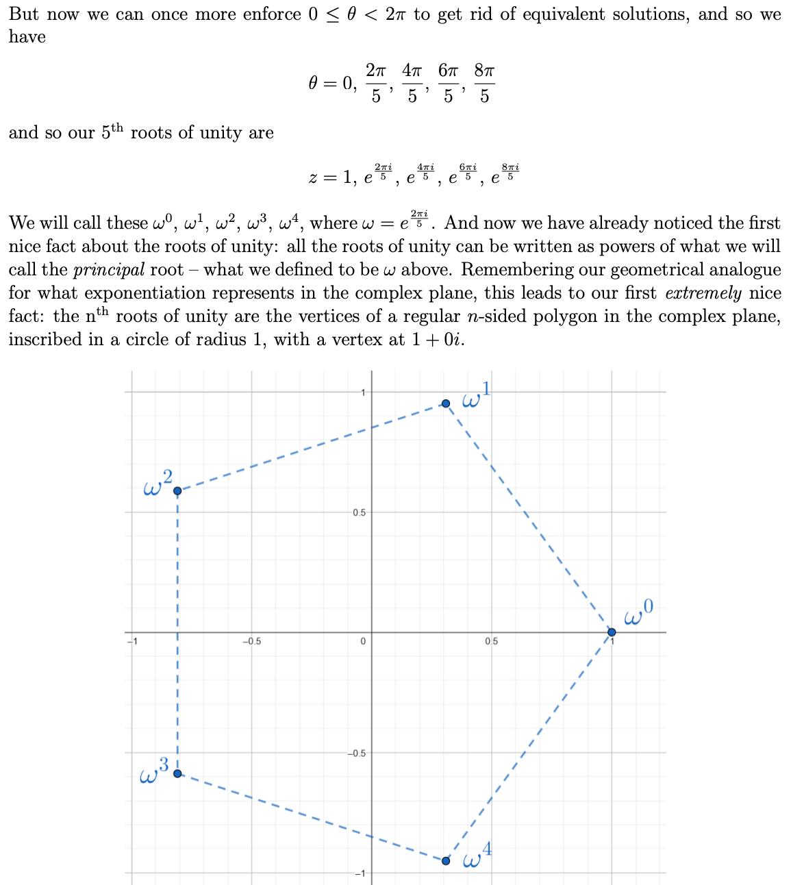
ROOTS OF UNITY: THE MOST BEAUTIFUL MATHS OBJECTS EVER
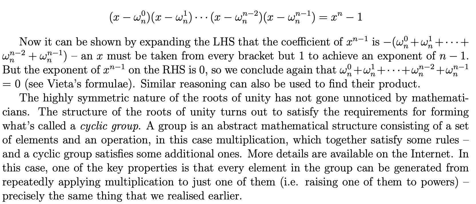
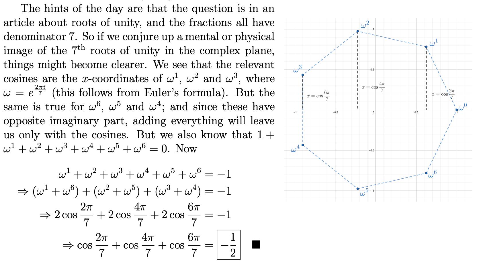
THE HIGHLY SYMMETRIC NATURE OF THE ROOTS OF UNITY HAS NOT GONE UNNOTICED BY MATHEMATICIANS THE STRUCTURE OF THE ROOTS OF UNITY TURNS OUT TO SATISFY THE REQUIREMENTS FOR FORMING WHAT’S CALLED A CYCLIC GROUP A GROUP IS AN ABSTRACT MATHEMATICAL STRUCTURE CONSISTING OF A SET OF ELEMENTS AND AN OPERATION, IN THIS CASE MULTIPLICATION, WHICH TOGETHER SATISFY SOME RULES –AND A CYCLIC GROUP SATISFIES SOME ADDITIONAL ONES. MORE DETAILS ARE AVAILABLE ON THE INTERNET. IN THIS CASE, ONE OF THE KEY PROPERTIES IS THAT EVERY ELEMENT IN THE GROUP CAN BE GENERATED FROM REPEATEDLY APPLYING MULTIPLICATION TO JUST ONE OF THEM (I.E. RAISING ONE OF THEM TO POWERS) –PRECISELY THE SAME THING THAT WE REALISED EARLIER.