SC PE


Dear Readers,
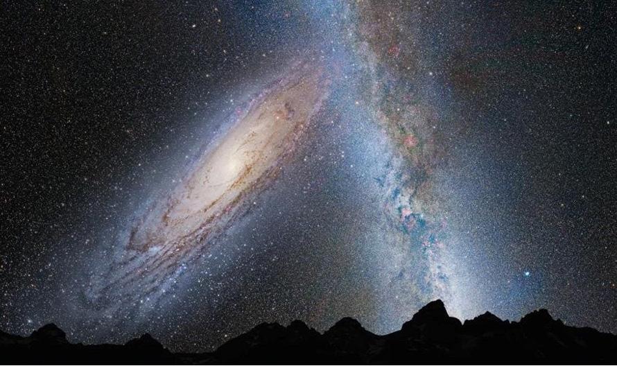
From the first spark of curiosity that ignites the mind to the profound revelations that reshape our understanding, the journey of discovery is an exhilarating one. As we celebrate this edition of SCOPE, we reflect on two monumental anniversaries that capture the essence of exploration: the 100th anniversary of the identification of the Andromeda Galaxy as a distinct entity, and the 50th anniversary of the Expanded Program on Immunisation (EPI).
A century ago, the discovery of Andromeda broadened our cosmic horizons, revealing that our Universe is not just a solitary expanse but a vast community of galaxies, each teeming with its own mysteries. This revelation propelled astronomers into a new era, one defined by the realisation that our place in the cosmos is part of a grander narrative. It ignited an insatiable curiosity, inspiring generations to look skyward and contemplate the Universe’s infinite possibilities.
Simultaneously, the EPI has transformed the landscape of global health over the last five decades. By ensuring access to vital vaccinations, it has saved countless lives and exemplified the power of science to effect positive change. This initiative highlights the critical importance of collaboration, innovation, and the relentless pursuit of knowledge in overcoming public health challenges.
In this edition, we weave together the threads of these two stories – one that looks outward to the stars and another that focuses on the vitality of human life. Our contributors have crafted insightful narratives that bridge the realms of astrophysics and immunology, showcasing how discoveries in one field can illuminate pathways in another.
As you journey through these pages, we hope you feel inspired by the interconnectedness of knowledge and the boundless potential that lies within our quest for understanding.
Warm regards,
Devarshi Mandal
Oliver West
Harishan Jenirathan
Nathan Wolfson
Student Editors
Dr Abda Staff Editor
Devarshi


Astronomical discoveries have continuously redefined our understanding of the Universe and the world around us, unravelling mysteries and creating more along the way. From the Assyrians and Babylonians as early as 1000 BCE to the Hubble Space Telescope revealing the true expanse of the Universe beyond us, astronomy has come a long way. Galileo’s telescopic observations introduced us to celestial dynamics and Kepler’s laws described planetary motion. Then there are the modern advancements, for example the discoveries of black holes and exoplanets. This scientist-led quest has brought us closer and closer to understanding the Universe’s structure – although, even now, we only understand a mere fraction of it (European Space Agency, 2019). Let us dig deeper into this cosmic journey and explore this vast web of astronomy woven by years of pioneering discoveries, opening the door into the wonders and discoveries that lie in front of us.
Let us begin in 1543 with a Polish man named Nicolaus Copernicus. He proposed his idea of the heliocentric model, challenging the earlier geocentric view (that the Earth was the centre of the Universe). In his model, Copernicus presented his idea of the Sun at the centre of the Solar System, and the Earth revolving around it (Westman, 2023). In fact, this idea was proposed as
early as the 5th century BCE by two Greek philosophers named Philolaus and Hicetas. These two men suggested that the Earth was a sphere revolving every day around a mysterious ‘central fire.’ Copernicus also suggested that the Earth turns once, daily, on its axis. Copernicus’ theories bought widespread controversy which even resulted in the Catholic Church issuing a prohibition against his theory (Finocchiaro, 2016). This eventually led to the condemnation of Galileo Galilei, whom we will move onto next, as a heretic.
Galileo’s telescope unveiled celestial secrets, such as previously undiscovered moons around Jupiter, and these advances reshaped astronomical understanding. Though Galileo was not the first inventor of the refracting telescope, he enhanced its capabilities massively. After he had started learning about telescopes, he began grinding and creating his own lenses and eventually created a telescope with a magnification of about eight or nine times. In due course, this telescope allowed him to see Jupiter’s satellites and the Moon’s mountains. He deduced the rough nature of the Moon’s surface by using the length of shadows (Royal Museums Greenwich, n.d.), additionally allowing him to estimate the length of lunar mountains. Apart from his discoveries of Jupiter‘s moons (now known as the Galilean moons), the stars of the Milky Way and the first pendulum clock, Galileo also made advances in understanding the phases of Venus.
Johannes Kepler was a German astronomer whose laws revolutionised astronomy. He precisely described planetary orbits and transformed our understanding when it comes to gravitational forces. In the early 17th century, Kepler suggested three laws of planetary motion (Gregersen, n.d.), basing his work on that already done by Copernicus, as mentioned previously. Kepler believed that Copernicus’ theory was not entirely accurate: for example, Copernicus described Mars to have a circular orbit, yet Mars actually has quite an eccentric orbit (the distortion of an ellipse is measured by a unit called eccentricity) in comparison to Earth. Kepler proved this experimentally and furthered the observations on the matter by his employer Tycho when he died in 1601.
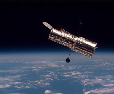
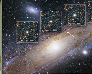
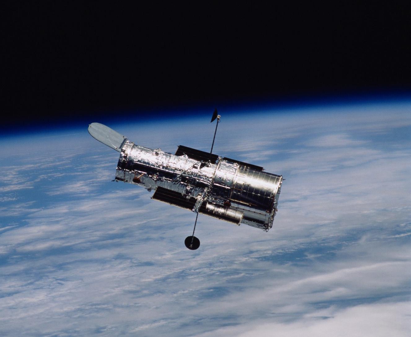
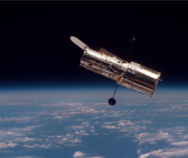
Edwin Hubble’s pioneering work laid foundations for our understanding of the evolution and structure of our Universe. Hubble had a deep love for Physics stemming from his childhood. He eventually went into astronomy and that astronomical journey took him all the way to the 2.54 metre Hooker Telescope (one of the largest telescopes at the time) in California (NASA, 2023). He used this telescope to observe faint patches of light which were known as nebulae. Hubble studied the Andromeda Nebula, which had never been seen clearly until Hubble ended up seeing individual stars in the nebula in 1923, thus discovering that it wasn’t a nebula but in fact a galaxy – the first known galaxy besides our own. Hubble kept studying Andromeda and went on to find more galaxies which he compared by their physical properties. Nowadays the Hubble space telescope soars high above the Earth continuing Edwin Hubble’s passion for searching the Universe in his own name.
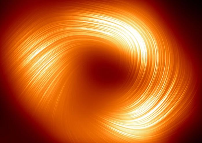
We move on to the enthralling topic of black holes, the thrilling yet enigmatic cosmic entities that have such an intense gravitational pull that not even something as fast as light can escape.
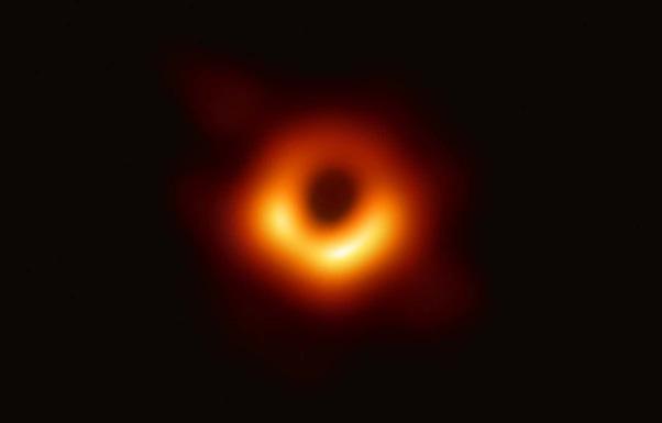
Black holes were first predicted by Albert Einstein in 1916, included in his theory of relativity. However, the term we all know, ‘black hole’, was coined by an American man named John Wheeler. The first signs of a black hole were observed in 1964 when a sounding rocket (a rocket designed for sub-orbital flights which carries instruments for collecting measurements) detected celestial X-rays (Space.com, 2023) (Tillman & Dobrijevic, 2023). In 1971, astronomers realised that the rays were coming from a blue giant which was orbiting a dark object – this object turned out to be a black hole. Black holes continue to be an area of wide research and of numerous new discoveries – for example, we have recently found that the closest black hole to the Earth, ‘The Unicorn’, may only be 1500 light years from Earth.
In the grand scheme of astronomical advancements, we have covered only a few: Copernicus’ heliocentric model, Galileo’s celestial insights, Kepler’s laws, Hubble’s studies into Andromeda and the black hole enigma – we never know what may be discovered next. These revelations have helped us further our understanding and knowledge of the Universe, reflecting humanity’s relentless pursuit of knowledge and the quest to figure out the mysteries beyond. In the complex world of astronomy, the thought of a future discovery is always present, as breakthroughs hold the promise of unveiling cosmic mysteries. Advanced telescopes could reveal dark matter or there could eventually be an answer to the centuries long debate concerning extra-terrestrial life. Investigating exoplanets and gravitational waves could reshape our lives, opening new frontiers in cosmic exploration.
Adam Smith SFH2
Galileo Galilei (1564-1642) was born in Pisa and educated in Mathematics and Natural Sciences, becoming Professor of Mathematics at the Pisan Studium in 1589. He made multiple discoveries throughout his life, all of which were revolutionary, hence challenging the accepted ideas of the time.
One of Galileo’s remarkable feats occurred in 1610 when
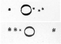
he directed his rudimentary, self-built telescope towards Jupiter. On January 7th of that year, Galileo noticed three points of light around Jupiter, and assumed that they were distant stars. However, over several further nights of observing Jupiter, he noticed that these points of light moved in a different fashion to the stars, remaining in proximity to Jupiter while exhibiting motion relative
to Jupiter. Continuing to monitor Jupiter, Galileo also discerned a fourth point following the same distinctive pattern of motion (Figure 1). On January 15th he concluded that these were moons of Jupiter rather than stars: a radical proposition considering the prevailing belief at the time that only Earth possessed a moon.
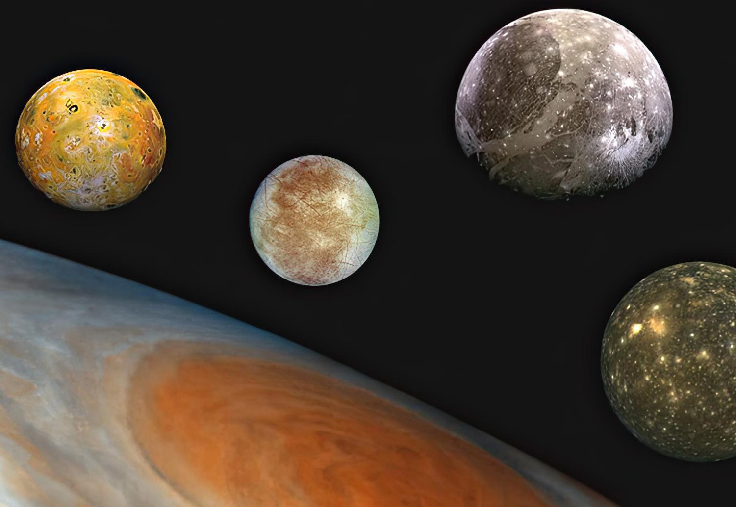
These four moons of Jupiter which we term the Galilean moons, were originally called “the Medicean Stars”, in honour of Galileo’s patron in the House of Medici, Cosimo the 2nd, the Grand Duke of Tuscany. They are now individually named after the lovers of Zeus (in order of proximity to Jupiter): Io, Europa, Ganymede, and Callisto. They all approximate the size of our moon, with Europa slightly smaller and the other three slightly larger. Ganymede is the largest moon in the Solar System and is larger than the planet Mercury (NASA, 2024).
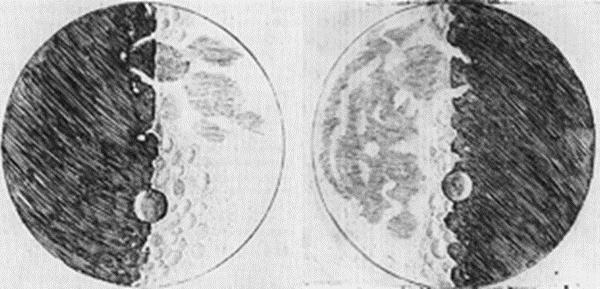
Galileo also observed our very own moon. The Moon was the only body in the sky that displayed discernible features to the naked eye, namely the Lunar Seas. The accepted belief of the time was that the heavens were perfect. But Aristotle argued that the features of the Moon were a result of it being corrupted by being close to the Earth. However, philosophers of the renaissance were disputing Aristotelian concepts (Del Soldato, 2023), views given credence by Galileo’s observation of the Moon. He saw far more details with his telescope, in the form of craters, mountains, and valleys (Austrailia Telescope National Facility, 2015). He observed their shadows on the Moon’s terminator (the line separating the day side from the night side) and through that deduced that the Moon’s surface was rough just like the Earth’s (Figure 2).
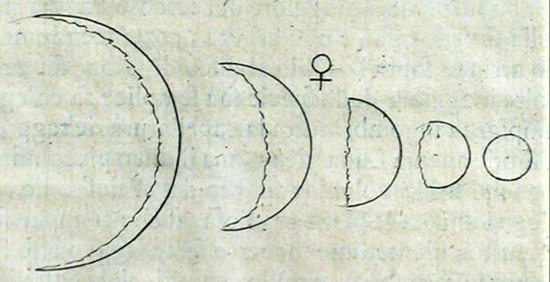
Another of Galileo’s groundbreaking discoveries was the description of the phases of Venus. Due to Venus’ greater proximity to the Sun than Earth, we can observe its distinct phases (the changes in the proportion of its surface being illuminated). Galileo was the first to discern these in 1610, documenting the varying size of Venus. He noted waxing phases during which its apparent size decreased, followed by waning phases during which its apparent size increased. This provided conclusive evidence that Venus orbited the Sun, as it changed position relative to the Earth and was illuminated by the Sun. This refuted the geocentric model as it showed that Venus orbited the Sun and not the Earth. Furthermore, it contradicted the idea that Venus was a ‘wandering star’, as was believed about the planets, a compromise to account for their motion relative to the stars. Mercury, like Venus, is a morning and evening ‘star’, and the discovery of the phases of Venus (Figure 3) suggested that Mercury had similar phases, although Galileo’s telescope did not have sufficient magnification to distinguish them due to Mercury being small and close to the Sun. This, along with Galileo’s discovery of the Moon’s rough surface, challenged the idea of celestial perfection, contributing to the understanding that Venus too was not a perfect object in the heavens.
2011).
Galileo also made a major discovery in 1610, observing what would later be identified as the rings of Saturn. Describing them as ‘handles’ on the side of the planet, he noticed that their shape changed, effectively disappearing as the Earth moved relative to Saturn. Galileo, unaware that these ‘handles’ were rings, referred to Saturn as a ‘triple-bodied planet’. It was not until Huygens (1629-1695) observed Saturn in 1659 that these features were verified to be rings, with Huygens also discovering Saturn’s largest moon Titan. Galileo’s observations clearly revealed distinct features on Saturn (NASA, 2011), and though they were not identified as rings at the time, it remains a momentous discovery.
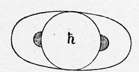
Figure 4: Galileo’s drawing of Saturn’s rings (NASA, 2011).
Galileo’s discoveries provoked significant discontent with the Establishment, especially with the Catholic Church as they conflicted with the contemporary church dogma, which asserted that everything orbited the Earth. Galileo published Sidereus Nuncius in 1610 in which he detailed his discoveries, from the Moon’s surface being rough, to the phases of Venus and the moons of Jupiter. 1613 marked the beginning of the controversies, with the Jesuitical Inquisition taking an interest in Galileo due to his theories.
Having been put on trial by the Inquisition (the church’s enforcers) in 1616, he was forced to recant his beliefs, effectively forbidding him from spreading his ideas. He was subsequently placed under house arrest in 1633, where he stayed until his death in 1642.
Despite attempts to muzzle him by the Establishment, Galileo’s discoveries continued to perturb the scientific community of the period, making geocentrism an untenable position. They similarly refuted the Aristotelian ideas about the perfection of the heavens, as they proved the Earth moves around the Sun, along with the other planets, and the Earth is not unique in its position in the sky. The observations of the Moon’s surface proved that the Moon was a celestial body like Earth. Considered in conjunction with the observations of Venus, this further proved that the other planets were bodies like Earth, as opposed to stars. This also led to the conclusion that they were not perfect bodies. The discoveries of the moons of Jupiter and the rings of Saturn showed that the other planets had moons of their own, and proved without a doubt that not everything orbits the Earth. The final death of Aristotelian perfection and geocentrism had to wait for Kepler and Newton (Kuhn, 1985). However, Galileo’s travails with dogma echo to this day (AHUJA, 2016).
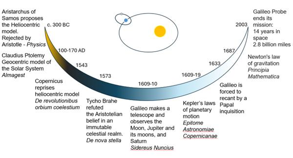
Three hundred and sixty-one years after the death of Galileo (Figure 5), NASA’s eponymous spacecraft completed its mission to Jupiter and its moons. Being unable to escape from Jupiter’s gravity, it was deliberately consigned to the planet’s surface; a triumph for the heliocentric model proposed by Nicolas Copernicus and made real by Galileo’s observations.
Figure 5: Diagram showing the timeline from geocentrism to heliocentrism. Items in italics are seminal publications.

Joshua Man SFS3
Introduction
The journey to understanding all of the intricacies under which our brains function remains an ongoing process, however, there have already been several notable findings that are important to reflect upon, not only due to their contributions to our knowledge of the brain, but also their
ground-breaking and crucial application in the real world. One such finding is the work spearheaded by Alan Hodgkin and Andrew Huxley, critically furthered by Sir John Eccles, which earnt the trio their Nobel Prizes in 1963 for ‘their discoveries concerning the ionic mechanisms involved in excitation and inhibition, in the peripheral and central portions of the nerve cell membrane’ (Curtis, 2015).
Alan
Having both been educated at Trinity College, Cambridge and briefly collaborated in 1939 before the Second World War, physiologists Hodgkin and Huxley reunited from 1946 to 1952 and formed one of the most influential partnerships in their field ever. Their work gave significant insight into nerve excitability, adding fundamental knowledge to the basis of what was understood of nerve action potential at the time – essentially, discovering how nerve impulses (the nervous system’s method of communication) are exchanged between cells. Whilst the two were working together with squid axons (the portion of a nerve cell that carries nerve impulses away from the cell body), an idea came to the physiologists to insert a fine capillary electrode inside the nerve fibre in order to record the potential difference across the membrane, as it was already understood that nerve cells used electrical impulses to communicate with each other (Schwiening, 2012).
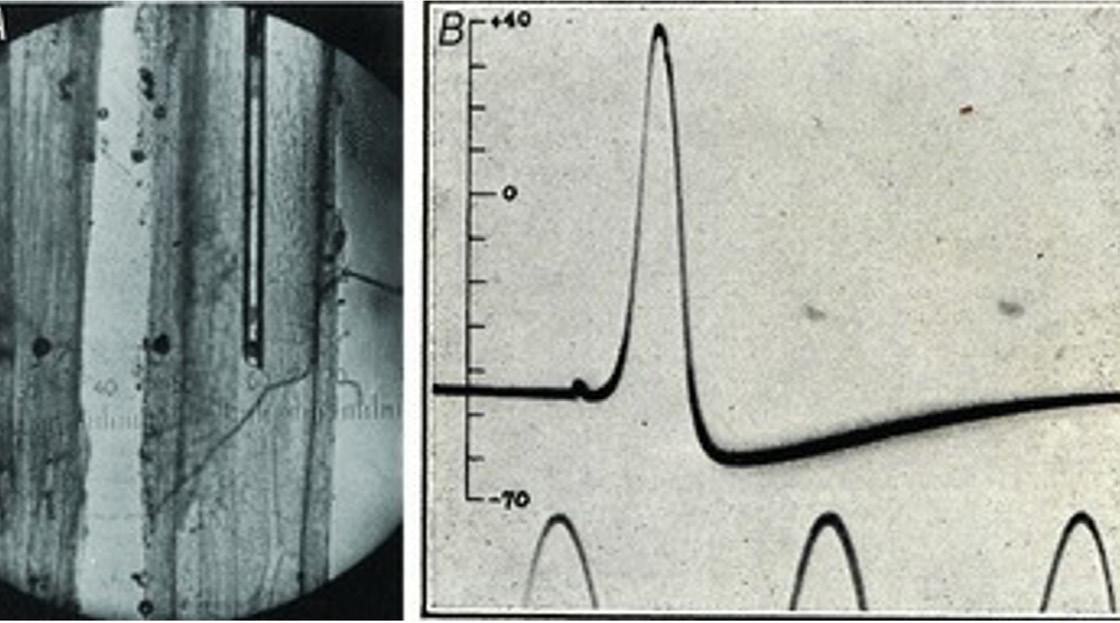
1: An electrode inside a squid axon (left) and a recording of the action potential in the axon (right) (Schwiening, 2012).
This was a groundbreaking achievement as it proved to be the first ever recording of an intracellular action potential, the basis of how information is transmitted throughout animals – and a large one at that. Specifically, the pair looked at the movement of potassium and sodium ions in their respective ion channels (proteins that allow charged ions to move in and out of a cell through the membrane, thus creating an electrical potential), and derived what is now known as the Hodgkin-Huxley (H-H) Model. This is a mathematical model linking microscopic ion channels
to the macroscopic level of currents or action potentials. Their equation was the ‘first complete description of the excitability of a single cell’ (Häusser, 2000).

1: The equation representing the Hodgkin-Huxley Model (Häusser, 2000).
This is widely regarded as their most remarkable achievement, owing to the study’s overarching influence across many disciplines and the efficacy of their experimental methods. With merely a few minor changes to the parameters, the H-H model could be used to describe a plethora of channel types, highlighting the wide application gained from this experiment. Furthermore, as is common with any strong theory, numerous other new experiments were to be carried out, inspired by the H-H model. For example, Armstrong and Bezanilla investigated currents related to the movement of gating particles in sodium channels. However, much merit in this experiment lies in the style in which it was conducted, effortlessly blending the theoretical and experimental together and using them to enhance one another until reaching a quantitative model for their experimental data (Häusser, 2000).
Australian neurophysiologist John Eccles earned his part of the same Nobel Prize as Hodgkin and Huxley through his work and research into synapses and the way in which nerve impulses are transmitted from one cell to another. In order to do so, he measured minute variations in electrical charges at contact surfaces between nerve cells – for the most part he looked at synaptic transmission in the CNS (Central Nervous System). Further research was conducted in the sympathetic ganglia (Haberman, 1972), which runs along the spine and is responsible for delivering information from the brain to the body regarding perceptions of danger.
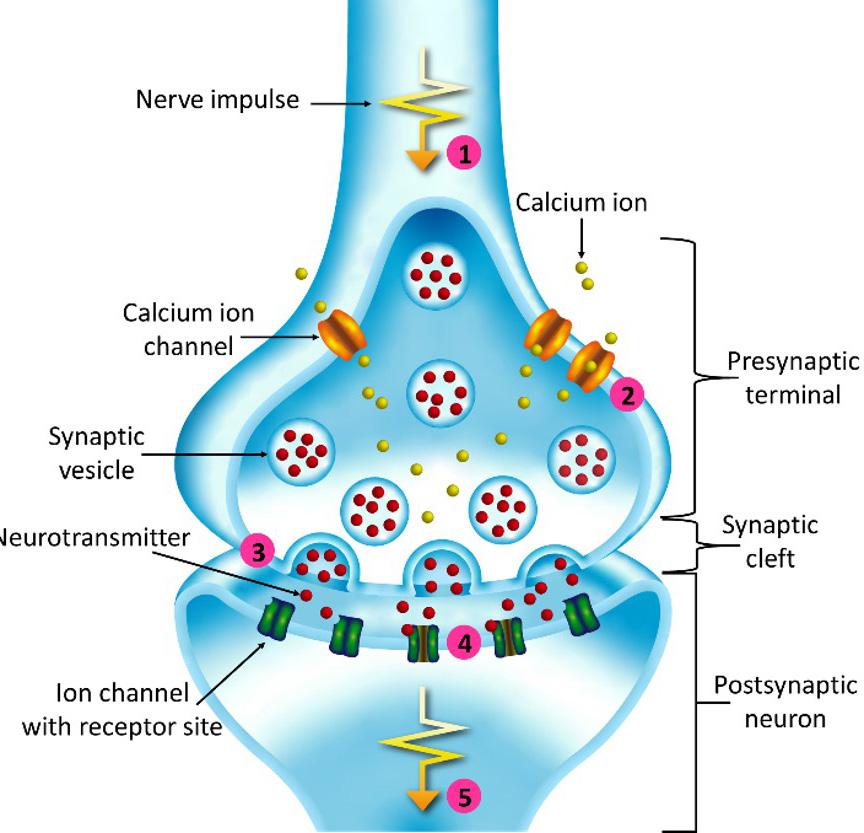
2: Action of neurotransmitters in the synaptic cleft (Okinawa Institute of Science and Technology, 2020).
Ultimately, the understanding of how action potentials in neurons are initiated and propagated that was provided by the H-H model has proved to be a massively significant milestone in developing our knowledge of the way in which our brain functions (Petousakis, 2022). The H-H model has been an indispensable tool for neuroscientists, paving the way for accurate and replicable modelling of the movement of ions in neurones, and the many phenomena that are facilitated by this. Similarly, the influence of Eccles’ work into the movement of electrical impulses across the synaptic cleft has spread far and wide, informing researchers in a myriad of enquiries. For example, the way in which antidepressants work as a treatment for clinical depression and OCD among other conditions, is heavily involved with synapses in our brain. Our brain releases serotonin, a neurotransmitter that has a significant effect on our mood along with other bodily functions, from the pre-synaptic neuron and travels across the synapse to bind to receptor sites on the post-synaptic neuron before being reabsorbed by the pre-synaptic neuron to be reused.
3: A serotonin molecule (National Center for Biotechnology Information, 2004).
The most common type of anti-depressants is Selective Serotonin Reuptake Inhibitors (SSRIs), and they work by blocking the reabsorption of serotonin (Figure 3) on the pre-synaptic nerve by binding to the reabsorption sites. This results in a build up of the amount of serotonin that has been released into the synapse that can continue to stimulate the post-synaptic neuron, with the desired effect of increasing or balancing out our mood. This alone is a massively important idea that Eccles’ work informed and stands among many other areas where his discoveries and those of Hodgkin and Huxley have been applied. Together, this trio fundamentally altered the way in which we understand how communication works in the brain and provided the groundwork for countless amounts of research and application to follow.
Introduction
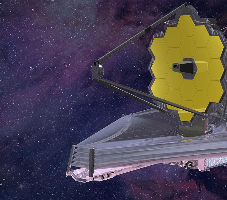
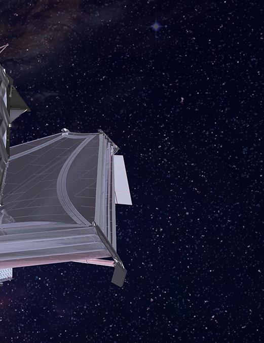
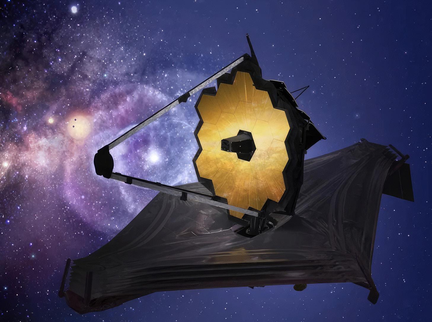
The James Webb Space Telescope is a multibillion-dollar space project worked on by Northrop Grumman, The National Aeronautics and Space Administration (NASA), and The European Space Agency (ESA). It took 20 years to make and faced seven years’ worth of delays until it launched on Christmas Day 2021. On that day it launched from Guiana and over the subsequent 30 days it travelled to the L2 point in space, also known as the
second Lagrange point, which is 1.5 million kilometres away from Earth (Northrop Grumman, 2023). It will stay at the L2 point for hundreds of years, though is only expected to remain operational for about 20 years. The telescope will hopefully give us an insight into how the world was created, as well as more fascinating pictures. The telescope can see 13.8 billion light years away (Royal Museums Greenwich, 2021).
The telescope is an engineering marvel and relies on some of the most complicated space technology we have seen. One of the most impressive feats are the gold mirrors, cleverly designed with hexagons (Figure 1), so that during the launch they could fold up sufficiently into the Ariane 5 rocket. The span of the 18 hexagonal mirrors, each 1.32 m wide, is equivalent in length to two tennis courts. The function of these mirrors is to focus on distant galaxies, which is extremely hard to achieve. To solve this issue, there are six actuators behind each mirror to achieve perfect focus for each mirror. Each primary mirror must be aligned with a precision of about 1/100,000th of a human hair (NASA, 2021).
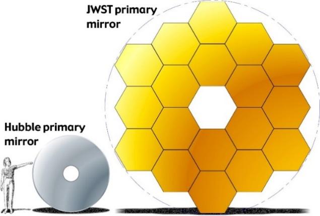
Figure 1: Comparing the sizes of the Hubble mirror and the JWST mirror to an average human (NASA, 2016).
As well as the mirrors, the telescope needs five main tools to operate (Figure 2):
1) The Fine Guidance Sensor (FGS) has a special system using different wavelengths to direct the telescope and keep it facing in the same direction to ensure the quality of the images it takes. The FGS operates at a 0.8-5 micrometre wavelength; for comparison, humans are able to see particles in the 50–60 micrometres range.
2) The Near Infrared Imager and Slitless Spectrograph (NIRISS) lets in only one part of the light to be diffracted instead of many. This tool is used to investigate light detection, exoplanet detection and characterisation, and exoplanet transit spectroscopy, which is a way to understand what the planet is and where it has been (NASA, 2021).
3) NIRCam, also known as the Near Infrared Camera, which operates at 0.6-5 micrometres, detects light from some of the earliest stars in the Milky Way and
objects in the Kuiper belt. NIRcam is equipped with a coronagraph, which allows astronomers to take pictures of fainter objects compared to more massive and bright objects like stellar systems. This is done by blocking the brighter object (NASA, 2021).
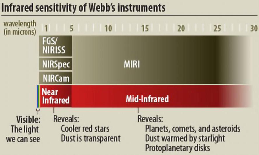
Figure 2: The sensitivity of the different tools to light (Phys org, 2016).
4) The NIRSpec (Near Infrared Spectrograph) operates at a wavelength of 0.6 to 5 micrometres. NIRSpec disperses light into a spectrum from which various information can be gathered, such as if it is a low temperature star or asteroid. However, the JWST must focus on the subject for over one hundred hours to see a readable graph of the spectrum. To help with this issue, scientists created a micro-shutter system capable of focusing multiple lights onto targets at the same time – the system has 250,000 shutters. In addition, it has a way of blocking all bright lights so that it can focus on more of the fainter lights that do not show up as easily on the spectrum (NASA, 2021).
5) The mid infrared instrument (MIRI) is a tool that is capable of penetrating the thick dust clouds that the telescope will most likely encounter. However, it will only operate at -266.5°C, so it uses a cryocooler to cool the telescope down to the designated temperature to stop MIRI from detecting the infrared radiation that it emits itself. The wavelength range of MIRI is 5 to 28 micrometres, so a lot bigger than the NIRSpec wavelength. It has many sensitive sensors which allow it to see redshifted light from distant galaxies and newly forming stars, as well as faintly visible comets. The camera provides a wide view image, resulting in breathtaking astrophotography (NASA, 2021). Similarly to the NIRSpec, the MIRI also has a spectrograph which allows it to collect more detailed physical details of the images it is viewing.
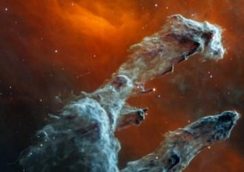
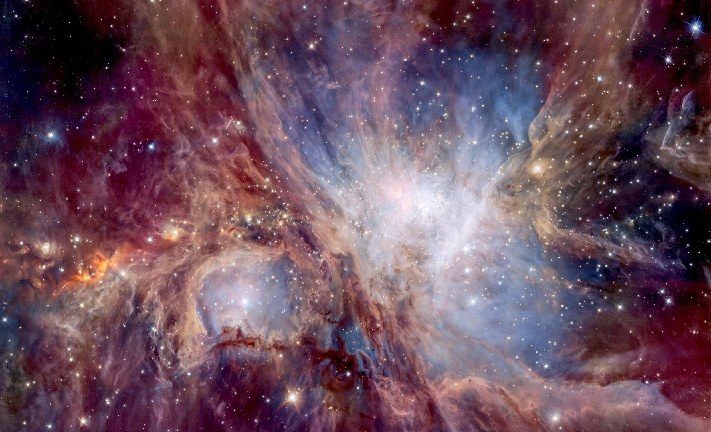
One of the big discoveries is stars being born in the Pillars of Creation, which is a nebula. The telescope managed to take a very impressive picture of the Pillars of Creation in the Eagle Nebula (Figure 3). The real discovery, however, lies in the smoky pillars, in which NIRCam on the telescope managed to capture exceedingly small red dots. These small red dots of dust and gas, bigger than our Solar System, are stars being born that are not yet burning hydrogen. The image itself is created using assorted colours to represent invisible wavelengths –most of the image to us would look like pure red.

Figure 3: Pillars of Creation (space.com, 2022).
Another brilliant discovery the telescope has made is the first ever image of an exoplanet. Scientists have known
about exoplanets since 1990, but the significance of this photo (Figure 4) is that it is the first ever direct image that has been taken of an exoplanet thanks to the incredible technology such as NIRCam and NIRSpec onboard the telescope.
“This is a transformative moment, not only for Webb but also for astronomy generally,” said Sasha Hinkley, professor of Physics and Astronomy at the University of Exeter (Fisher, 2022). The planet is named HIP 65426 b. Notably, the distance between the planet and its host star is 92 astronomical units (92 times the distance from the Sun to the Earth), making it further away from its sun than any planets in our Solar System (space.com, 2022).
The James Webb Telescope has a lot of potential to look further into our Universe and explore areas that are over a trillion miles away. With the new capabilities offered by this telescope, astronomers hope to uncover things like how our Solar System was created and how the first stars came to be.
The James Webb Telescope has already made groundbreaking discoveries, and with the technology and potential that the telescope holds, we hope to see more big breakthroughs uncovering the secrets of our Universe.
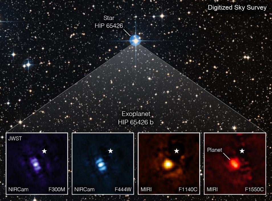
Figure 4: HIP 65426 b The telescope’s first direct image of an exoplanet - HIP 65426 b. (space.com, 2022).

Richard Zhou 11R1
This article examines the possibility of a Mars colony project and demonstrates that there are a variety of problems which will be encountered along the way, and that each problem can be combatted scientifically using recent breakthroughs in research and technology.
In recent years, Mars has attracted great attention from the international community. With the successful 2020
Could
advancements
landing of the Mars rover Perseverance, Mars is one of the most promising goals for humanity to achieve, and the ISS (International Space Station) has already made plans to make further landings on the surface of the red planet. A permanent establishment on Mars would satisfy insatiable scientific curiosity and provide an opportunity for more in-depth observational research.
Among all extra-terrestrial bodies in our Solar System, Mars stands out as the only planet that has abundant resources to support life (Zubrin, 1996). Its mantle is plentiful with
technology finally make a Mars Base possible?
magnesium, iron, calcium, nickel, sulphur, and potassium (Anon., n.d.). Its geography is also very similar to Earth, with volcanoes, ice caps, seasons, weather, underground water deposits and a day hardly longer than ours. The new environment present for Martian humans will also greatly benefit evolutionary change in humans, which will help support a new branch of human civilisation. Whilst initially being quite difficult to adapt to, the harsh conditions on Mars may cause genetic mutations in humans residing there for long periods of time (Learn, 2021). This leads to better adaptations, such as skin cells which can withstand higher quantities of radiation and are less likely to be cancerous. Our new, improved adaptations would be of benefit if our aim is to become an interplanetary species and deal with a variety of climates. In addition, becoming an interplanetary species will also decrease our own extinction rates, increasing our survival chances as a species.
The primary obstacle for our Mars colony would be to create a breathable atmosphere and find the means of feeding and hydrating our space travellers. Due to the lack of elements present on Mars, there are only a few chemical reactions which can produce oxygen:
• MOXIE process
• Sabatier reaction
Recently, NASA scientists have developed a process called MOXIE (Mars Oxygen In-Situ Resource Utilization Experiment). MOXIE takes in carbon dioxide from the Martian atmosphere through a HEPA (high efficiency particulate air) filter, compresses it, heats it to 800 °C and applies solid oxide electrolysis directly to carbon dioxide, splitting and decomposing carbon dioxide (CO2) into
carbon monoxide (CO) and oxygen (O2), which provides a stable supply of oxygen (Hoffman, 2022).
The problem is that carbon monoxide does not have many uses and is toxic to humans, requiring an extraction system to remove it safely.
Another solution is the Sabatier reaction: CO2 + 4H2 ACH4 + 2H2O, through nickel-based catalytic reduction at temperatures of 300-350°C. The water (H2O) is then electrolysed to produce hydrogen (H2), and breathable oxygen (O2).
A great benefit is that the carbon dioxide reactant could be directly imported from Earth via pressurised cylinders on spacecraft, which subsides our climate problems, whilst replenishing our Mars colony’s oxygen and water supply. Methane (CH4) acts as a good rocket fuel, and water could be used and recycled, or broken down into oxygen.

All this work will be no good if we simply cannot feed our space travellers. The Martian atmosphere is unfortunately too thin, and too dry for plants to survive in. However, there remain a few ways of growing food:
• Lab grown meat.
• Greenhouse grown plants.
• Growing plants in lunar regolith.
Growing meat without the need to nurture and shelter a whole animal will be greatly advantageous to our colony and could feed our astronauts very well. In 2019, a company called Aleph Farms demonstrated how to easily create lab-grown meat, without the need for multiple animals. The process involves extracting living cells from an animal and then growing these cells in bioreactors, with the help of nutrient serums, which over time can produce fully grown meats. This method has proven successful, and Aleph Farms unveiled the very first labgrown ribeye steaks a few years back (Tomaswick, 2020). However, the process requires huge chemical input and a lot of time, and it may be difficult and dangerous to transport chemicals onto Mars from Earth.
Another option is to use greenhouse grown plants to our advantage. They are naturally bioregenerative and can use light energy to create oxygen, remove carbon dioxide and synthesise food. We could also condense the
water they transpire into pure form, meaning they could contribute to our water purification system. To make this viable, we could construct greenhouses to support our plants, with specially adapted environments like that on Earth.
Finally, growing plants in lunar soil (regolith). For the first time ever, in May of 2022, NASA scientists at the University of Florida discovered that plants could grow in the layer of unconsolidated deposits (regolith) obtained from the surface of bedrock on the Moon (Keeter, 2022). This ground-breaking discovery could mean that under the correct conditions, Martian regolith may be able to support plant life, allowing for the expansion of plant farms in our colony.
A largely self-sustainable Martian colony would, at present, be theoretically feasible through a variety of new technological advancements and innovative designs that make them possible. However, the Mars base is still a long way from being perfect, especially considering risk factors such as finiteness of resources, unpredictable dust storm patterns and difficulties in communication should a problem arise with the systems, but as solutions to these problems are proposed, we will likely see bases being set up within the next one or two decades and the future is highly promising.

Introduction
In this article, I aim to unravel the mystery of cryptography, an art and science that has been around for 4000 years. From Ancient Rome to WW2, from Queen Elizabeth to Alan Turing, it has played a major role in shaping history as we know it. This article will explore the foundation of classical cryptography, and its modern implementations in today’s world of technology.
Encryption is the process of converting text to an uninterpretable string of characters, and the study of this is known as cryptography, with people developing
encryption techniques being known as cryptographers. This can be used for a variety of reasons, but the main application is when sending confidential information over a distance. This is to keep the content from being understood by third parties, even if intercepted. It may be used in letters, emails, computer systems, and even government communication. Any text that we want to encrypt is known as plaintext, which is the original form that can be understood by anyone who reads it. The text is then enciphered into a ciphertext. The method used to encipher the text is known by the intended sender and receiver so that, once received, the original plaintext can also be retrieved.
Encryption methods can generally be divided into two categories, transposition and substitution. Transposition is re-arranging the characters/words within a text. For example, the text ‘HELLO’ could be transposed to ‘OLLEH’. On the other hand, substitution involves replacing characters/words with other characters/words. For example, ‘HELLO’ could be substituted with ‘XPSST’. When it involves replacing entire words, it is known as a code, and replacing characters is simply known as a cipher. Steganography is the process of hiding text. As this doesn’t involve scrambling text, it doesn’t come under the header of cryptography. People may also combine various encryption methods together to make their data even more secure.
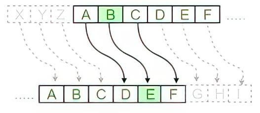
A feature of many ciphers is that they incorporate a key, which is an additional piece of information needed to encipher and decipher the message. An example of its usage can be seen in the Caesar cipher, whose key is a digit from 1 – 26. It is a substitution cipher, and each letter is shifted in the alphabet by the key number, as shown in Figure 1. For example, the word ‘CAESAR’, with a key of 3, results in the text: ‘FDHVDU’. Three letters on from C gives you F, three letters from A gives you D, and so on. If the letter Z is reached, you would loop back to A. In order to decipher the message, you would go back in the alphabet by the key number. Three letters back from F gives you C, three letters back from D gives you A, until you reach the original, decrypted text: ‘CAESAR’.
If an unwanted recipient manages to intercept a ciphertext with the Caesar cipher method applied, they should be unable to decrypt it without knowing the key. We now have a successful method of encryption. However, this
subsequently came with the desire to unravel encrypted texts without knowing the key. Cryptanalysts were people who developed ways of doing this, known as cryptanalysis. The most basic form of cryptanalysis is using the bruteforce method. This involves going through each of the possible keys until an appropriate plaintext is produced. For example, on ‘FDAVU’, you would try:
• Key = 1 to receive ‘ECGUCT’
• Key = 2 to receive ‘DBFTBS’
• Key = 3 to receive ‘CAESAR’.
Realising key = 3 gives a recognisable word, this is likely to be the shift used in the original cipher.
As a result, many more complex methods of encryption evolved, making it harder to perform cryptanalysis. For example, while the Caesar Cipher may only take up to 26 attempts, some others may take many years to solve using brute-force. Thus, the desire for more advanced cryptanalysis and tougher encryption methods has been an ongoing battle for many centuries. Examples of advanced cryptography are Vigenère and Hill Ciphers, while more advanced cryptanalysis methods include Frequency Analysis and the usage of Cribs (part(s) of the original plaintext already known).
With computers becoming increasingly more advanced, two issues arise with classical cryptography, the first of which is the ability to efficiently decrypt text. While manual brute-force by hand may be unrealistic, computers processing billions of instructions per second could uncover ciphertexts almost instantaneously. This issue can be avoided by implementing keys of larger sizes.
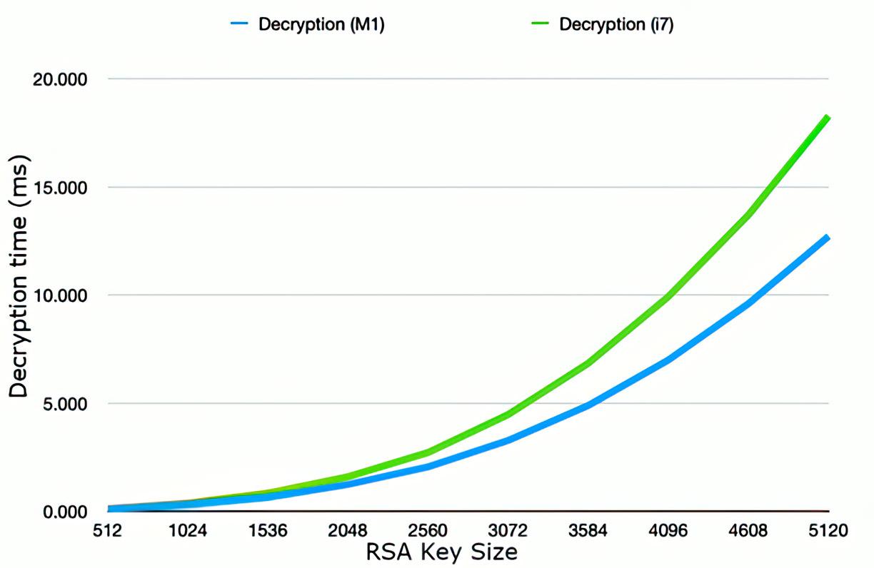
Computers store and process information using 0s and 1s, known as the binary system, with each digit being known as a bit (binary digit). Electronically, a computer translates the binary system with an inactive wire representing 0, and a live wire representing 1. Therefore, using a key of length 1 means only two possible [0 and 1] pieces of information can be used. However, increasing the key length exponentially increases the number of possible keys. Using just 50 bits allows 250 (a quadrillion) unique keys. This relation is demonstrated in Figure 2, showing the correlation of key size to decryption time for two example ciphers.
The second issue is regarding the distribution of the key. Traditionally, it would be agreed on manually or in person. However, today, it would be impractical to visit your email recipient and physically implement the key on their computer. As a result, some computers began sharing the key over the internet. However, this raises another problem. Just as an eavesdropper might be able to intercept the ciphertext, they would also be able to obtain the key, thus making encryption redundant. The solution to this problem can be achieved using a process involving one-way functions.
A one-way function is a mathematical calculation which is easy to perform one way, but difficult to reverse. This can be represented with the following analogy: Given two colours, a human could easily identify the resultant colour just by mixing them together. However, it would be a lot trickier to reverse the process and figure out the original colours used to make it. Simple maths functions such as doubling don’t fulfil this requirement. For example, doubling 8 to give 16, is just as easy as halving 16 to give 8. On the other hand, multiplying two primes such as 229 and 197 might be easy, but it is a lot harder to factorise 45113. This would be an example of a one-way function. One-way functions can be implemented in two ways. The first of which is using it to create a secret key known only by the sender and receiver. This can be used for any encryption method. An example of such an algorithm is Diffie-Hellman.
So far, we have looked at algorithms which use symmetric
logic. For example, to decrypt a Caesar Shift of 5, you would go back in the alphabet by 5 letters. Other encryption algorithms use one-way functions as the basis for encryption itself. This is known as asymmetric encryption. Using one-way functions, you can make a cipher which requires two separate keys: an encryption & decryption key. The encryption key is able to convert plain text to cipher text, but can’t reverse the process, because of one-way algorithms. However, the decryption key is mathematically linked to the encryption key at their creation, so it is able to easily reverse the process. An example of one-way functions using asymmetric encryption is the RSA method.
In conclusion, it is evident how fast the development of ciphers has grown, and how mathematically complex they have become. Encryption as an entirety has proved its importance throughout time, yet no cipher has managed to find itself permanent. At the time of writing, the standard encryption methods have been stable for several years. However, with scientific advancements, and data being widely available via the internet, it is only a matter of time before we figure out how to properly manipulate quantum cryptography. At that point, the race between cryptographers and cryptanalysts will continue: the battle for the last ‘unbreakable’ cipher, for the safety of our data. Data is information and information is power. Whoever can decrypt the data, holds the power!
The Global Positioning System (commonly referred to as GPS), since its inception by the United States Military in 1973, has become an irreplaceable tool in the current information age dominated by global internet infrastructure. It is used in multiple high-level applications, including locational tracking, major communication networks, banking systems, financial markets, and power grids. The functions of a GPS are heavily utilised to ensure these applications perform with near-absolute accuracy and it has been an invaluable tool in the modern era of technology.
The functions of a GPS include being able to pinpoint 3-dimensional position to metre accuracy, and time to the 10-nanosecond level 24/7 and across the world (Manning, 2023).
The most notable founding scientists who significantly contributed to the development of the GPS include:
• Roger L. Easton, who pioneered the GPS predecessor program known as TIMATION (Time Navigation). Its purpose was to demonstrate the ability to place highly accurate clocks into orbit, to advance time measurement (increasing the number of sites sharing the same precise time measured), and to allow for successful twodimensional navigation. Its revolutionary success led directly to the creation of the GPS program (Singh, 2023).
• Dr Ivan Getting, one of the main supporters of the GPS program. He worked in the administration-related areas, proposing as well as planning and negotiating with all the system’s stakeholders to allow GPS to become a reality.
• Dr Bradford Parkinson, who was at the forefront of the NAVSTAR GPS team (NAVSTAR is the previous name for GPS) tasked with finding altitude, latitude, and longitude for navigation, using the TIMATION’s work with clocks and TRANSIT’s (US Navy satellite type) orbital prediction method.
• Dr Gladys West, who overcame massive adversity in a male-dominant industry to process lots of data from satellites to pinpoint their location, eventually programming an IBM 7030 to provide calculations for a geodetic Earth model (which provides accurate measurements of the Earth), which was refined further to become the GPS orbit (Hardy, 2023).
The Global Positioning System consists of three parts critical to its function: the Space Segment, Control Segment, and the User Segment.
The Space Segment comprises a constellation of satellites, both legacy and modern generations transmitting radio signals to users. This transmission is produced by the transmitter component, and is received by an antenna on the device, which is often small and unnoticeable. These satellites are arranged into six equidistant orbital planes surrounding the Earth – the location of these satellites means users can view at least four satellites from any point on the planet. A recent upgrade to this constellation system means there are at least 27 satellites instead of 24 satellites used, providing improvements in GPS performance across most parts of the world.
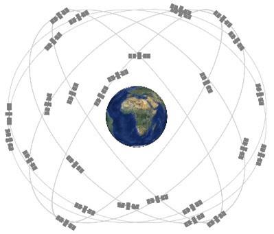
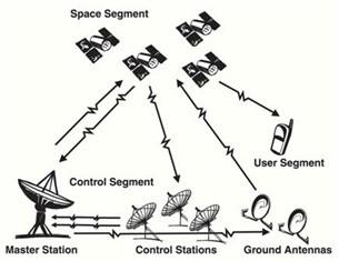
Figure 1: Expandable 24-slot satellite constellation, as defined in the SPS Performance Standard (GPS.GOV, 2019).
LNAV Message Structure (Typical data structure of GPS messages):
Sub-frame Word Description 1 1-2
TLM (Telemetry) and HOW (Handover) words.
3-10 Satellite clock; GPS Time Relationship.
2-3 1-2
TLM (Telemetry) and HOW (Handover) words.
3-10 Ephemeris
4-5 1-2
Figure 2: Interaction of all 3 segments (Sfrcollege.edu.in, 2014).
The US Space Force also frequently update the satellites used. Satellites in operation between the 1990s and early 2000s had a feature termed “Selective Availability”, which is the scrambling of the satellites’ clocks, reducing the accuracy of C/A (Course/Acquisition) code transmitted to the user (and so GPS accuracy lowers). Only in the last decade, this “feature” was removed, after recognition of its hinderance of the development of GPS technology and its world impact.
As part of the user segment and transmission of signals three PRN (Pseudorandom Noise) ranging codes are transmitted: the precision (P) code which is the principal navigation ranging code; the Y-code, used in place of the P-code whenever the anti-spoofing (A-S) mode of operation is activated (antispoofing is the prevention of the legitimate GPS signal from being transmitted); and the coarse/acquisition (C/A) code which is used for acquisition of the P (or Y) code (denoted as P(Y)) and as a civil ranging signal, also known as variant signals (Eoportal.org, 2024). These codes allow any receiver to identify exactly which satellite is receiving.
To provide the time and position, ephemeris (precise orbital information) and almanac (low-resolution orbital information) for each satellite, GPS encodes this information into the Navigation message, modulating it to C/A and P(Y) ranging codes. In the case of the legacy navigation messages, known as LNAV, they utilise more modern formats which have very similar structures, leading to slight differences in structure. A Navigation message is composed of 30 second frames which are 1500 bits long, divided into five 6 second subframes of 30-bit words each – words are specific sequences of bits pertaining to different functions relating to the signal (Psu.edu, 2023).
TLM (Telemetry) and HOW (Handover) words.
3-10 Almanac (including error correction).
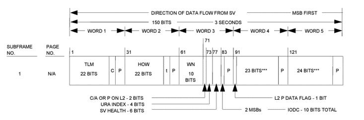
Figure 3: Example Structure for LNAV Subframe 1 (NAVSTAR GPS Interfaces (IS-GPS-200), 2019).
The combination of PRNs and LNAV (or its variants) interact with the User segment, providing information related to the operation of the GPS i.e. pinpointing 3-dimensional position and time. The User segment is how GPS is applied in many scenarios, such as in aviation for flight safety, farming, construction, mining, surveying: from smartphones to shipping containers.
The last aspect of GPS is the Control Segment. This consists of a large global network of ground facilities that track the GPS satellites, monitor their transmissions, perform analyses, and send commands and data to the constellation, and is controlled by the National Oceanic and Atmospheric Administration – a USA Government Agency that ensures that the GPS constellation of satellites continue to deliver high performance (GPS.GOV, 2019). These include Monitor stations which record and send the operational data of active satellites. At these stations, the complex GPS receiving method known as differential GPS is utilised which eradicates error. All data is then provided to the Master Control station which analyses all provided data, and relays instructions back to satellites via Ground Antennas.
To conclude, the GPS is a highly complex, interconnected system which is operational due to the aforementioned three segments: Space, User, and Control. Despite early development for military purposes, it has been repurposed as a hidden gem for humanity to progress in the current technological era, and in future applications such as predictive maintenance and asset tracking in businesses while increasing overall accuracy
Mathematicians are sometimes berated for spending a lot of time studying things with seemingly no application to the real world. While physicists find new sources of energy to fulfil humanity’s needs, chemists design and manufacture new drugs to cure every illness under the sun, and biologists innovate medical techniques to extend human life, mathematicians sit in offices scrawling notes and writing papers on some of the most abstract and esoteric problems known to humankind – problems which, more often than not, they have made up for their own entertainment. And yet it seems to be a strange inevitability that no matter how obscure the enquiry upon which mathematicians embark, no matter how seemingly removed from real life,
it sooner or later comes back to provide huge value to all of us, and sometimes even underpins the world that we come to take for granted. The mathematician G.H. Hardy said in 1940, “No-one has yet found any war-like purpose to be served by [number theory] or relativity or quantum mechanics, and it seems very unlikely that anyone will do so for many years” (Hardy, 1940); and it was with an almost vindictive rapidity that these fields proved their real-world applicability, with number theory becoming the foundation of modern cryptography and relativity and quantum mechanics shaping the future with the development of the atomic bomb. Perhaps there is no more canonical example of such an application than what has been called ‘the most important numerical algorithm of our lifetime’ (Strang, 1994) – the fast Fourier transform.
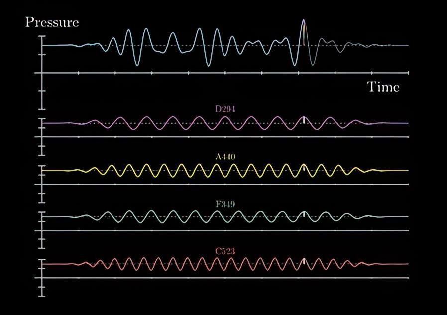
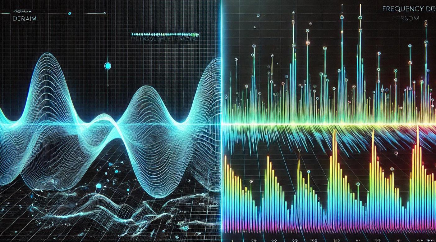
The normal Fourier transform is a mathematical process that is used to decompose a function into the pure frequencies that add together to make that function. Mathematically, it can be shown that every periodic function (i.e. any function that eventually repeats) can be expressed as a (potentially infinite) sum of sine and cosine waves at some frequency, where the frequency is simply how often the wave’s value passes above and below 0 (Weisstein, n.d.). For example, in Figure 1, we see that the apparently complicated wave at the top can in fact be written as the sum of four sine and cosine waves – and these sine and cosine waves, perhaps surprisingly, can be reverse engineered given only the wave that they sum to create. This process is the Fourier transform.
While the idealised Fourier transform for mathematical functions is often useful in, for example, the solution of certain types of equations, its cousin, the discrete Fourier transform (DFT), is unbelievably useful for a huge range of applications (Smith, 1997), such as providing approximate solutions to equations, fast algorithms for important mathematical functions (Weisstein, n.d.), lossy image compression, and most importantly, signal processing. The normal Fourier transform is too abstract to be applied
to real-world, discrete data, but the DFT is specifically designed for real-world data – and it turns out that there are a huge number of situations where it is very helpful indeed to know the pure frequencies that add to make a function.
One often-cited instance where the demands of the real world have actually stimulated the development of new mathematics is the discovery of the fast Fourier transform (FFT) in a five-page paper by Cooley and Tukey (Cooley & Tukey, 1965). As the story goes, during nuclear disarmament talks between the United States and Soviet Union, the major barrier to progress was the difficulty of reliably detecting nuclear tests from across the world, and thus the impossibility of ensuring the other side had truly ceased from carrying them out. The DFT provided a potential solution – if seismometer readings could be decomposed into their constituent frequencies, then certain frequencies indicative of nuclear explosions could supposedly be identified to conclude whether or not such tests were taking place (Rockmore, 2000).
There was just one problem. One way to view the DFT is as a matrix-vector multiplication, which is just a fairly common type of mathematical operation. However, viewing it this
way, it becomes clear that to perform a DFT on n data points would take in the order of n2 slow multiplications – for a series with 1 million data points, 1 trillion multiplications would be needed, which is prohibitive even for modern computers, let alone Cold War-era machines.

Figure 2: FFT as a factorisation into sparse matrices.
However, the realisation of Cooley and Tukey can be viewed as the fact that the DFT matrix, denoted F above, has certain symmetries which allow it to be factorised into a series of sparse matrices, denoted Si, which are significantly faster to multiply (Loan, 1992). Namely, the Fourier transform of the data series x, Fx, can be calculated by first finding S0x, which is just a vector, then multiplying this by S1, etc. Each multiplication only takes n operations instead of n2, due to the sparsity of the matrices, and the factorisation produces m = log2n such matrices. This means the total number of operations required is in the order of nlog2n, which is far, far fewer than n2 before – for example, when n = 1 million, we now need only around 20 million operations, which is well within the range of feasibility.
You might ask, then, why we are not inhabiting a nuclear weapon-free world given that this discovery enables us to detect nuclear weapons tests on the opposite side of the world with relative ease. It was in 1963 that the US and Soviet Union’s refusal to allow inspections of their nuclear facilities resulted in only a partial ban, for all tests except underground ones, being prohibited (U.S. Department of State, n.d.). But it wasn’t until 1965, two short years later, that Cooley and Tukey published the algorithm that could have resulted in a complete test ban, had the relevant parties not already left the negotiating table . Indeed, the nuclear arms race was soon joined by France and China alongside the UK, US and USSR, with the result that a treaty banning underground tests wasn’t instituted until 1996. Since that point, India, Pakistan and North Korea, all
non-signatories to the ban, are the only countries to have carried out nuclear tests (Arms Control Association, n.d.).
Furthermore, it was observed in 1966 that the necessary ideas to reach the FFT had already been conceived as early as 1942, but were simply not well-known and not fleshed out enough to be applied to seismometry (Rudnick, 1966).
The greatest shock of all was yet to be had, however, as it became clear that an FFT algorithm as powerful as Cooley and Tukey’s had been found by Gauss in 1805, but, being written in an abstruse form of modern Latin and with many notational quirks, had been all but forgotten, with many special cases being rediscovered over the subsequent years and also being disregarded. Perhaps, if we had only paid more attention to what Gauss had been up to in 1805, the algorithm that is now so essential to modern life could have become widely known 160 years earlier.

When Alice stepped through the mirror in Lewis Carroll’s “Alice Through the Looking Glass” she found a world that was a mirror image to normal. In this reflected world, clocks tick the opposite way and writing is back to front. Alice poses the question: “Is looking-glass milk safe to drink?”
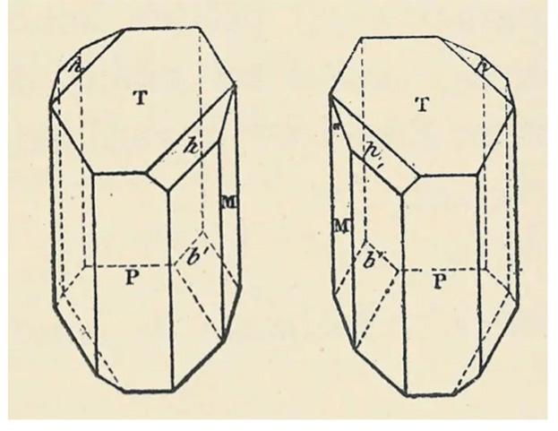
If you placed both of your hands directly on top of each other, you would find that they are non-superimposable despite being mirror images. This quality is called handedness or “kheir” in Greek. Louis Pasteur coined this term in the 19th century to describe optical isomers in a sample of paratartaric acid, as shown in Figure 1 (Klein, 2017):
“We say that non-superimposable objects that are mirror images exhibit “chirality”. Therefore, all asymmetric objects exhibit this property, and we call such objects enantiomers (optical isomers).”
In this article, we will explore whether the effects of inverting chirality in a simple glass of milk are enough to cause significant detriment and harm to the body. To answer this question, we must first analyse the composition of milk and ask whether its different parts demonstrate chirality, then discuss the potential effects of this phenomenon, noting that most biological molecules do in fact possess enantiomers (Inaki, et al., 2016).
“Whole cow’s milk contains about 87% water. The remaining 13% contains protein, fat, carbohydrates, vitamins, and minerals. Cows are often pregnant while they are milked, so dairy milk also contains hormones like insulin-like growth factor-1 (IGF-1), oestrogens, and progestins.” (Willett & Ludwig, 2021)
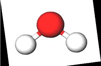
Water has a line of symmetry through the oxygen atom, so is superimposable and as a result achiral (it does not exhibit chirality).
So, looking-glass water is identical to normal water, and thus interacts normally with the human body. That means that 87% of looking-glass milk is completely safe to drink, and that high percentage might mean that there is a low enough concentration of other chiral molecules for them not to cause much damage, even if they are harmful.
2:
Proteins on the other hand, do exhibit chirality. In fact, the only amino acid that is achiral is Glycine, because it has two hydrogen groups attached to the central carbon, but for a molecule to be chiral, it needs to have four different groups on a carbon.
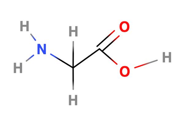
3: Glycine has two hydrogens around the central carbon, so is not chiral.
Because all other proteins have complex R-groups instead of a simple hydrogen, most proteins exhibit chirality, for example lactate, which has two enantiomers, as shown in Figure 4.
But if proteins exhibit chirality by default, why wouldn’t they also demonstrate a 50:50 mixture of their different isomers by default (we call this 50:50 mixture of isomers a racemic mixture). Surely, if a 50:50 mixture was to be inverted, nothing would change.

Figure 4: The two enantiomers of lactate (Pollegioni, 2019).
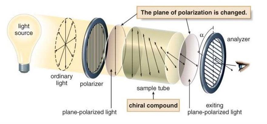
Sadly, this isn’t the case. Amino acids are differentiated into two types of enantiomers: Levorotatory and Dextrorotatory amino acids from the Latin “levo”left and “dextro” - right (Inaki, et al., 2016). They are differentiated based on how they manipulate polarised light (Figure 5). When light is polarised, only wavelengths travelling in one direction pass through the polariser. These wavelengths then pass through a sample tube with the molecule. The sample rotates the light to the left if it is a Levorotatory sample, and to the right if it is a Dextrotatory sample. No change in rotation is observed if it is a racemic mixture.
This kind of experiment has helped deduce that most proteins are composed of L-amino acids (one enantiomer only) because enzymes preferentially synthesise and break down L-amino acid variants. This is a clever biological mechanism to ensure that the organisms only ever need to deal with one enantiomer. So, looking-glass milk will have these L-amino acids mirrored to become D-amino acids. Enzyme synthesis and breakdown systems in the human body are specifically designed for L-amino acids, therefore the D-proteins probably won’t fit into their respective enzymes.
We can observe this by looking at enzyme substrate complexes. The active site of an enzyme is specifically shaped to fit a particular protein. When the shape of that protein changes, it is possible that the protein will no longer fit the active site of its corresponding enzyme. However, another model for enzyme-substrate interactions (the induced fit model) details that a substrate must only roughly fit the active site and the enzyme will then change shape to accommodate the substrate. It is important to note, even here, that the fluctuation of shape is very minor, and probably won’t account for the total inversion of proteins in looking-glass milk. This is quite concerning when considering that biological enzymes can recognise chiral molecules as very different substances (Nguyen, et al., 2006). We will consider this idea later.
Do lipids exhibit chirality? Glycerol and fatty acids are both achiral, but when the first (C-1) and third (C-3) fatty acids are different in a lipid, the second (C-2) becomes a chiral centre, so the molecule exhibits chirality. Milk contains hundreds of different lipids, only some of which have been identified (Liu & Rochfort, 2023). The majority of these species have different C-1 and C-3 groups, so exhibit chirality.
Other things we must consider are:
1. Do the lipids in milk make a racemic mixture?
2. If not, are chiral enantiomers safe?
One might assume that lipids are simple enough not to involve the protein specific enzymes present in protein synthesis. But lipid synthesis is actually incredibly complicated.
Enzymes are involved in lipid synthesis. In a process known as “secretory differentiation”, acyl-CoA: diacylglycerol acyltransferase (DGAT) and acyl-CoA: cholesterol acyltransferase (Inokoshi, et al., 2009) enzymes are produced from within the endoplasmic reticulum.
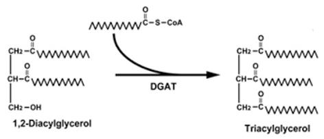
Their function is to synthesise triglycerides and cholesteryl esters that are present in the lipid core. The former can be expressed as two isozymes (which are isomers and enzymes). The discrepancy between the isomers of these triglycerides seems to lie in the products they form (namely triglycerides or cholesterol-based compounds), not the chirality of the molecule.
Thus, it seems logical to conclude that overall, the enzymes involved in lipid synthesis can demonstrate the same preference to laevorotatory enantiomers as demonstrated in protein synthesis and that lipid breakdown and synthesis systems are designed only for one chiral enantiomer, and therefore lipids do not form racemic mixtures in milk. This seems to suggest that the dextrorotatory enantiomer won’t fit into enzymesubstrate complexes and won’t be broken down (Hamosh, et al., 1985) (McManaman, 2009).
However, because of the sheer number and variance in types of lipids, the body’s breakdown mechanisms for dealing with chiral isomers of lipids has to be nonspecific to the lipid itself, so the chirality of the molecule is negligible.
How does this non-specific mechanism work? Lingual and gastric lipases begin the breakdown of lipids by catalysing the hydrolysis of their fatty acids (Martin & Freedman, 2014) to produce 1,2-diacyl-sn-glycerol and free fatty acids. This is non-specific, because all lipids have a glycerol bonded to fatty acids, so the hydrolysis
of fatty acids at the glycerol group is independent of the length of the fatty acid or any other lipid-specific factors. This in turn produces a long list of catabolic enzyme reactions that are non-specific to the type of triglyceride. To summarise, because a chiral lipid will still contain fatty acid chains (just in a different order), the mechanisms for their breakdown will remain the same, meaning that looking-glass lipids are safe to consume.
Vitamins also exhibit chirality, but it seems that there are cases where chiral vitamins only perform their function less effectively instead of causing a different effect. Take Vitamin E for example (Bogdan, et al., 2008): our bodies have a high preference for the isomer α-tocopherol, but that doesn’t render the other enantiomers useless, just less effective. Similarly, the binding affinity of Vitamin D is highly dependent on which enantiomer is present (Terauchi, et al., 2018). Different enantiomers in vitamins affect potency but not necessarily their function.
Most minerals are monatomic (e.g. potassium, magnesium, calcium, zinc), which in turn means they are symmetrical. This means they do not exhibit chirality so are safe to consume in looking glass milk.
Nutritionists and biologists have already been considering the dangers of foreign hormones in our bodies. Hormones are chiral, but their effect is probably negligible. According to an article by Hassan Malekinejad (Malekinejad & Rezabakhsh, 2015):
To evaluate a hormone “as a potential hazard for humans and animals, a few critical points should be” considered:
1. We must accurately determine the “amounts of free and bound forms of naturally occurring hormones”.
2. We must ask what “percentage of determined hormones are absorbed via gastrointestinal tract and consequently, what percentage of absorbed hormones undergo hepatic biotransformation.” This “will provide a clear picture of bioavailability of each individual hormone.”
We can see that two factors affect the danger of potentially hazardous hormones: the amount of free unbound hormones, and the concentration absorbed in the gastrointestinal tract. With regards to the number of hormones present and percentage of the milk, they both seem small enough to be considered negligible, and thus the effect of hormones can be ignored.
Are chiral proteins and vitamins safe? This question is beyond graduate learning, but I will try and estimate and predict their effect by looking at case studies and other considerations.
Firstly, it seems evident that “L-enantiomers can be far more dangerous than D-enantiomers” (Crump, 2022) because of their effect on the body. D-enantiomers generally aren’t incorporated into the body, so just won’t form enzyme substrate complexes. Because the majority of the enantiomers in looking-glass milk are of the D-variation, this means that they can be safely egested by the body. This highlights the first possible reaction our bodies can have: no reaction at all.
For example, one isomer called the “(S) enantiomer” of Ibuprofen has the desired pharmacological activity, but another isomer (called “the (R) enantiomer”) is completely inactive (Nguyen, et al., 2006). This is supported by Easson-Stedman’s illustration of the hypothetical interaction between the two enantiomers of a racemic drug. The inactive drug is unable to bind to receptors and so has no functional role.
On the contrary, there’s the infamous thalidomide. One enantiomer of thalidomide was designed to cure morning sickness, whilst the other caused teratogenic birth defects in children when consumed by pregnant women.

It is rather difficult to gauge the effects of certain chiral molecules on the body, and whilst a glass of chiral milk might be completely safe, we must conclude that there are too many potentially chiral components that can affect the body’s processes. Similarly, assessments like these have become an integral part of gauging the safety of drugs during development. In a world that faces increasing drug complexity and thus an increase in the permutations that the shape of a molecule can take, perhaps we will see an increase in development times for drugs, as a result of warranted precaution around chiral isomers.
how it was discovered and what it tells us
Hari Das 11C2
Introduction
Almost 60 years ago on May 20th 1964, two scientists Arno Penzias and Robert Wilson, in the process of calibrating the Holmdel Horn Antenna at Bell Telephone Laboratories,
heard a faint hissing sound emanating from the sky. This discovery would later be identified as the Cosmic Microwave Background Radiation, the remnants of the first light from the Big Bang, and the origin of the Universe.
Originally conceived for NASA’s project Echo, an early attempt at global satellite communication, the Horn Antenna was designed to operate by leveraging satellites to radio waves. The Horn Antenna was subsequently tasked with detecting these reflected radio waves. However, the launch of the Telstar satellite quickly rendered the system obsolete, prompting Penzias and Wilson to repurpose the antenna as a radio-telescope, requiring calibration. During this process, the two scientists encountered a disruptive background noise which drowned out the radio signal the machine was meant to receive. Penzias and Wilson initially believed this to be a fault with the machine, an assumption which led them to chase nesting pigeons from the machine and put tape over every protruding rivet. In Penzias’ own words he expressed: “When we first heard that inexplicable ‘hum,’ we didn’t understand its significance (Chodos, 2002), and we never dreamed it would be connected to the origins of the Universe” (Wall, 2014). Indeed, it was only when they had exhausted all other options that they considered they had discovered something new. One observation they made while attempting to eliminate the sound was that its intensity and frequency did not decrease but rather remained constant throughout the year; an observation which led them to theorise that the sound was extra-galactical in origin. This idea was crucial, motivating them to contact Robert Dicke - a physicist concurrently postulating the idea of the Big Bang - who confirmed that the sound was the Cosmic Microwave Background Radiation (CMBR). This revolutionary discovery would later earn Penzias and Wilson a Nobel prize, shared with the Russian physicist Pyotr Leonidovich Kapitsa for unrelated work (The Nobel Foundation, 1978).
When the announcement of the CMBR was made, it provided significant support for the Big Bang theory, surpassing the Solid-State theory which posited that the Universe has and will always stay the same. The discovery of the CMBR coupled with the observations of Hubble has provided scientists with irrefutable evidence for the Big Bang theory (Tegmark & Efstathiou, 1996), establishing it as the widely accepted model for the origin of the Universe. The CMBR is a remnant of the first light of the Big Bang. These light waves gradually
underwent red-shift due to the expansion of the Universe - a phenomenon involving their wavelengths lengthening over time until they shifted out of the visible spectrum, and into the lower frequency band of radio waves, thereby spreading out their energy over a larger area. The sheer age of the waves serves as evidence of their origin in the Big Bang. Following the initial discovery, further research was conducted concerning the radiation. One such example is the analysis of the different minute changes in the radiation, used to infer properties of the early Universe such as density and energy. The CMBR has also been employed to estimate the age of the Universe. However, despite this discovery, questions persisted regarding whether changes in our position in the galaxy would impact the intensity and constancy of the CMBR. The NASA COBE mission, designed to gather additional data on the CMBR using space-based observatories rather than ground-based ones, later addressed this question and many others. This mission confirmed that CMBR is homogenous or similar in all directions, inspiring a flood of smaller-scale experiments in the Earth’s stratosphere, collecting supplemental data on the CMBR (Lineweaver, 2003). These further observations allowed scientists to take the data and create a detailed map of temperatures and densities of the very early Universe. More recently, scientists have discovered gravitational waves embedded in the CMBR; an occurrence they believe serves as a smoking gun for evidence supporting the Big Bang. Looking to the future, the potential discoveries that the CMBR can offer us are vast and we likely have not even scratched the surface.
In conclusion, the discovery of CMBR was an incredible achievement, fueled by scientific cooperation, curiosity and a healthy dose of luck. This discovery told us more about the birth of our Universe and will fuel scientific discovery for decades to come.

The advent of consumer plastics in 1907 by Leo Baekeland is undoubtedly one of the greatest advancements in human history. Baekeland, a Belgian-born American chemist, is often referred to as the “father of the plastics industry” due to his invention of Bakelite in 1907. Bakelite was the first synthetic plastic, meaning it was not derived from plants or animals. Baekeland’s creation was revolutionary because it was durable, heat-resistant, and could be moulded into almost any shape. This invention laid the foundation for the modern plastics industry and opened the door to the wide variety of synthetic polymers we use today. The following year, a team at ICI’s (Imperial Chemical Industries) plant in Winnington were attempting to combine ethylene and benzaldehyde. The experiment failed due to a leak of oxygen into the vessel. Upon further investigation, they found a white waxy substance in a reaction tube. This was found to be a polymer of ethylene. Now the world’s most abundant plastic, polyethylene was a wonder material: strong, flexible and heat resistant. Discovered by accident.
Could
ever create a plastic that decomposes?
Plastic is now one of the most ubiquitous materials available to both consumer (Rannard, 2023) and industrial applications and critical to the success of many industries. The benefits of plastics extend beyond their technological applications; they play a vital role in the economic development of emerging countries. In regions where access to traditional materials is limited or costly, for example Mozambique, plastics offer affordable yet versatile alternatives for manufacturing, infrastructure, and consumer goods. By their nature, plastics are lightweight and durable making them ideal for transportation and packaging, reducing transportation costs and extending the shelf life of perishable goods. Additionally, plasticbased products for agriculture such as water storage containers or irrigation systems enhance productivity and quality of life in resource-constrained settings.
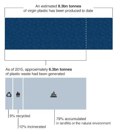
Unfortunately, this all comes at a very well understood cost. The very feature that makes plastic such an incredible resource, its durability, is also the reason why we can’t keep using it in the way we currently are. 4.9 billion metric tons (Parker, 2018) of plastic currently sit in landfill and will continue to stay there for up to 500 years. It is for this reason that the matter of decomposable plastic could be one of the simplest solutions to such a great problem.
The environmental impact of plastics is also profound, particularly in terms of pollution and contributions to climate change. One of the most pressing issues is bioaccumulation. Plastics break down into microplastics, which are small enough to be ingested by marine and terrestrial organisms. These microplastics can accumulate in the food chain, starting from plankton and moving up to larger fish, birds, and even humans (Gallo, 2018). This accumulation can lead to toxic effects as plastics often contain additives such as phthalates and bisphenol A (BPA), which are known endocrine disruptors (Figure 2). The presence of microplastics in the human body is linked to various health issues, including hormonal imbalances and increased cancer risk.

The chemical structure of plastics, which is mostly composed of large, strongly bonded molecules called polymers, prevents them from breaking down. These polymers give plastics their durability and long-term stability as they are made up of repeating units joined by strong covalent bonds. In addition, a lot of plastics are made to withstand environmental elements including rain, direct sunlight, and microbiological activity. Applications like construction materials and packaging that demand long-term durability will benefit from this resistance to deterioration. But it also means that plastics continue to pollute the environment and deteriorate it long after they are supposed to be used. Despite continuous research into biodegradable substitutes, plastics’ intrinsic resilience poses a substantial obstacle to the solution of the plastic waste problem (Smith, 2018).
Scientific innovation in sustainable plastic waste management encompasses a broad spectrum of strategies, from advanced recycling techniques to the development of biodegradable materials. Enzyme-based recycling represents a significant breakthrough in the management of plastic waste, offering a sustainable alternative to traditional mechanical and chemical recycling methods. This approach leverages the catalytic abilities of enzymes to break down polymers into their monomeric units, which can then be recycled to create new plastic materials.
One of the most promising innovations in this field is the development of highly specialised enzymes, such as PETase (Parker, 2018), which can efficiently degrade polyethylene terephthalate (PET), a common plastic used in bottles and textiles. Researchers have also engineered mutant enzymes with enhanced activity and stability, further improving the efficiency of plastic degradation. The process involves the enzyme binding to the plastic polymer at specific active sites thus destabilising the polymer chains, leading to their breakdown into smaller, recyclable molecules. The formation of these enzyme substrate complexes is highly specific, meaning that enzymes can be designed to target particular types of plastics, minimising contamination and improving the purity of the recycled output. This specificity not only enhances the recycling efficiency but also reduces the environmental impact, as the enzymatic process
ever create a plastic that decomposes?
operates under mild conditions, requiring less energy and producing fewer byproducts than conventional methods. Furthermore, the advent of chemical recycling provides a pathway to repurpose plastics that were previously considered non-recyclable, thus expanding the life cycle of plastic materials and minimising our reliance on virgin resources.
Research into decomposable plastics is passing through its infant stages. Several initiatives, such as the BioRisk Plastic Project are developing materials that are inherently degradable under natural conditions, designing synthetic plastics that can be broken down by microbacteria. Biodegradable polymers are being conceived as replacements for traditional plastics. These products are obtained from renewable sources that range from plant starches to cellulose, or even microbial fermentation byproducts. These biopolymers can be engineered to mimic traditional inorganic plastics, having the same properties and processing capabilities but, crucially, also be prone to digestion by micro-bacteria. With this natural propensity, getting rid of them is easy and microorganisms, bacteria and even the enzymes they secrete can efficiently break down the biodegradable plastic into its building blocks. Other research efforts concentrate on making existing plastics more prone to microbial or enzymatic degradation with chemical modifications or additives. By encapsulating enzymes known for their microbial digestion properties, researchers can create plastics that better withstand the most severe states of use, while still effectively being broken down into their smallest components inside a microorganism or enzyme bath after relevant disposal.
Efforts are ongoing into designing a material where the main component is naturally degradable, thus enabling longer lifespans for traditional or increased recyclability after the materials have been used once. Besides the research activity devoted to the development and initial use of decomposable plastics, another batch of researchers
is now testing these products, running lifecycle analyses to determine the environmental footprints of decomposable plastics, and understanding the biodegradation kinetics. The ultimate goal of biodegradable plastics is simple: to reduce plastic pollution and lower the environmental footprint of plastic waste. Biodegradable plastics offer a glimmer of hope but are overshadowed by numerous concerns. While it would be beneficial if these polymers served as inexpensive alternatives to traditional oilderived plastics, this isn’t always the case. In countries with inadequate waste management infrastructure, might it not be more practical to continue using traditional plastics? This approach could sidestep the initial costs associated with implementing biodegradable plastics.
While it is clear that we have made significant inroads towards a more sustainable future with bioplastics, it simply isn’t enough, yet. The longer it takes to implement this technology, the worse our waterways, ecosystems and landfills will get. We need a significant global push towards better science in the space of biodegradable plastics. Unless we act, 12bn tonnes of plastic waste will end up in our landfills and waterways by 2050, which would be the final blow in any attempt to save our planets biodiversity. All hope is not lost however, for example, the UK government will set the world’s most ambitious climate change target into law to reduce emissions by 78% by 2035 compared to 1990 levels, and many governments are now taking ownership over their individual roles in kerbing plastic pollution. We are certainly on the right track, but it will require a continued collective effort to ensure that we begin to reverse the damage that has been done to our ecosystems.
decomposes?
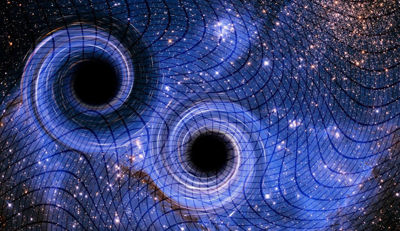
Gravitational waves were not discovered all at once.
It has taken half a century for humans to develop the technology to detect them, and it took nearly a century to directly observe them. Yet, even after all this time, we have not uncovered all their secrets.
In this article, I will discuss the various discoveries that have led to our current understanding, starting from Einstein’s general relativity and culminating in the main discovery made by the LIGO (Laser Interferometer Gravitationalwave Observatory) recently. I hope this article will demonstrate how many brilliant minds have contributed to this field, each making their own discoveries and gradually advancing our understanding of the Universe.
The concept of gravitational waves originated in 1916, emerging from Einstein’s theory of relativity, which posited that gravity is not an instantaneous force after all and gravitation propagates at a finite speed - the speed of light. This theory suggested that cataclysmic events such
as collisions between black holes or neutron stars would produce invisible yet incredibly fast ripples in space, now known as gravitational waves. Initially, the idea seemed peculiar, and even Einstein, the architect of the equations that predicted their existence, initially dismissed it, doubting that such a peculiar consequence of his theory could manifest in the real world (LIGO Lab, n.d.-a).
A significant development related to gravitational waves occurred in 1974 when Russell Hulse and Joseph Taylor of Princeton University discovered the first pulsar in a binary system using the Arecibo radio telescope in Puerto Rico. By analysing the arrival times of pulses from the pulsar, they provided conclusive evidence of gravitational waves, for which they were later awarded the Nobel Prize. This marked an important milestone toward directly observing gravitational waves, offering an indirect glimpse of their effects. However, at that point, gravitational waves had yet to be directly detected, leaving some lingering doubts about their existence (LIGO Lab, n.d.-a).
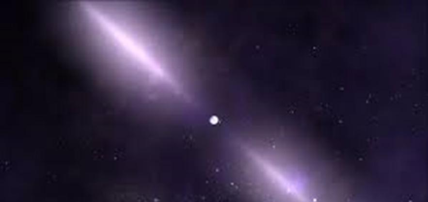
In 1984, a joint Caltech/MIT project was established to detect gravitational waves as predicted by Einstein’s General Theory of Relativity. The workings of the LIGO interferometer are incredibly intricate. In essence, the LIGO interferometer splits a light beam from a single source in half. Each beam travels down an arm perpendicular to each other, bounces back and forth off two mirrors before returning to be reunited with its partner at a detector. Along the way power recycling mirrors are added to strengthen the laser. By then studying how the beams interfere, we can determine if a gravitational wave has passed (Silver, 2017).
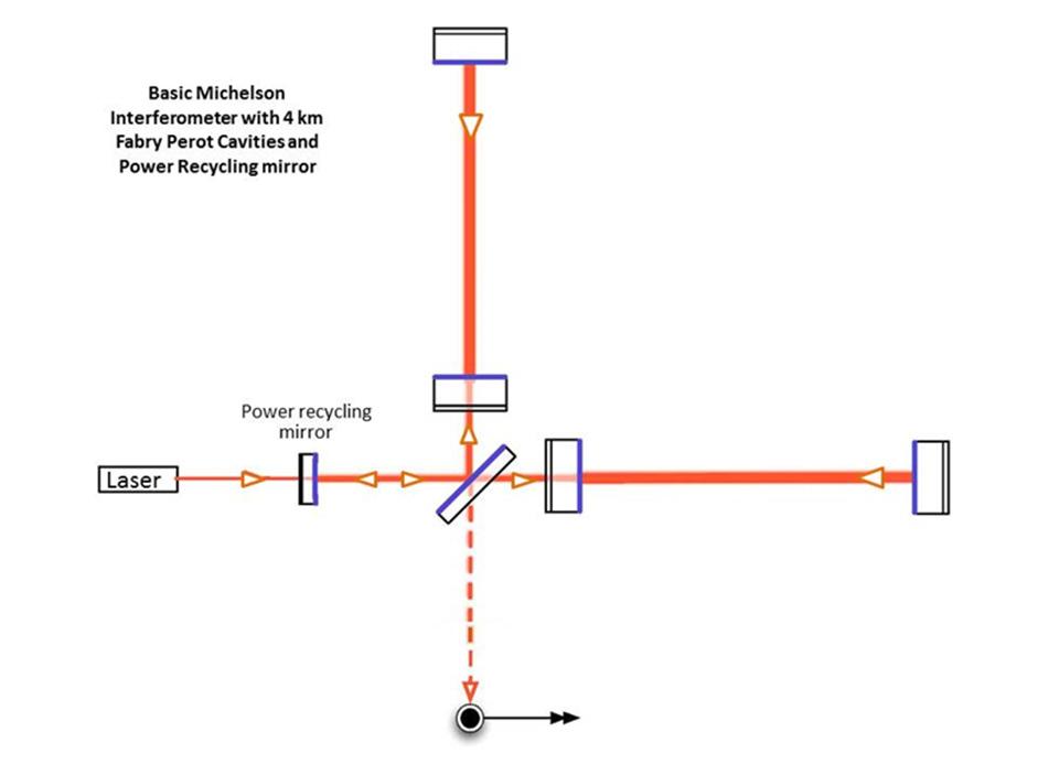
Figure 2: A diagram of a basic Michelson interferometer (LIGO Lab, n.d.-b).
In the LIGO interferometers, as long as the two beams travel the same distances, then when they recombine, they interfere destructively, and no light comes out of the instrument. This is what happens when there is not a gravitational wave. However, in the presence of a gravitational wave, the interferometer’s arms also oscillate in length, thus causing the lasers within them to travel different distances before recombining, resulting in their light waves no longer being perfectly aligned and some light leaking out. This proves that the gravitational waves cause spacetime itself to oscillate, alternately stretching in one direction while compressing in a perpendicular direction. These oscillations last as long as the wave is passing (Silver, 2017).
When the peaks of two waves meet, their peaks add up (constructive interference). When the peaks of one wave meet the valley of another identical wave, they cancel out (Figure 3 shows total destructive interference) (LIGO Lab, n.d.-c).
The pioneering experiments taking place demanded stringent precision requirements. Its mirrors had to be
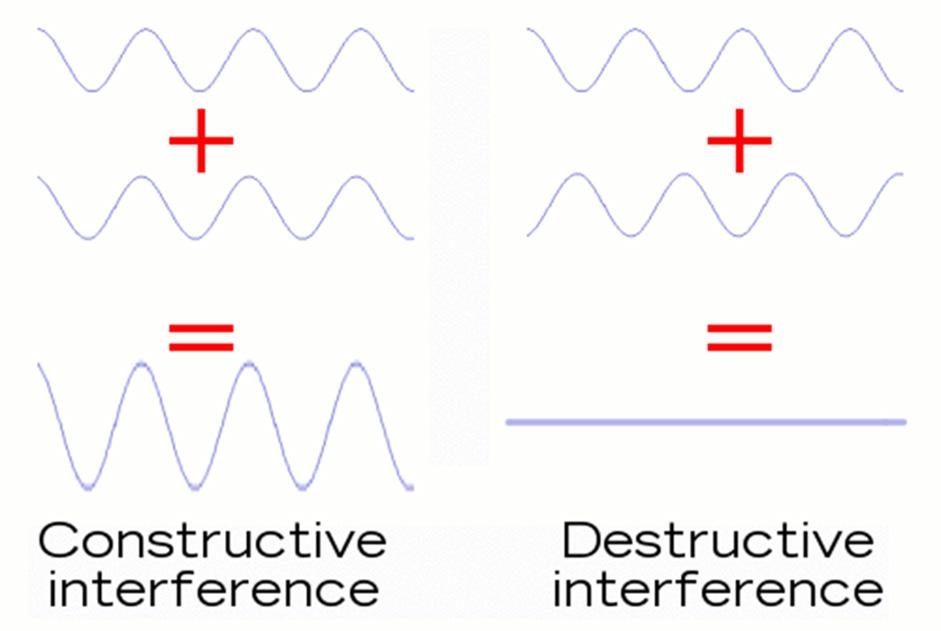
Figure 3: A graphic demonstrating constructive and destructive interference (LIGO Lab, n.d.-c).
flawless, its light beams exceptionally powerful, and it required the second-largest vacuum environment, meticulously shielded from sound or light interference to prevent experimental disruptions (LIGO Lab, n.d.-d).
To offer some perspective, the power used to operate the LIGO complex equated to just under 1 megawatt, sufficient to power six hundred homes (LIGO Lab, n.d.-b). It took 40 days to reduce the atmospheric pressure within the LIGO interferometer’s vacuum to one trillionth of normal atmospheric pressure (LIGO Lab, n.d.-e).
Furthermore, the setup of the LIGO complex was duplicated to minimise the risk of false positive detection. The entire project incurred a cost exceeding 400 million dollars. Eventually, this concerted effort and investment paid off on September 14, 2015, when scientists at LIGO headquarters finally detected a gravitational wave, 99 years after its initial prediction by Einstein (LIGO Lab, n.d.-a).
The gravitational wave detected by LIGO’s interferometers resulted from the merger of two black holes 1.3 billion lightyears away, generating an energy burst 500 times more powerful than anything else in the observable Universe. For this groundbreaking discovery, three individuals involved in the LIGO complex were awarded the Nobel Prize, along with sharing a 1-million-dollar prize (LIGO Lab, n.d.-a).
So, what’s the significance of this discovery? Gravitational waves have opened a new ‘window’ on the Universe. Things like colliding black holes, which are utterly invisible to normal astronomers can be studied and their properties may be explored. More importantly, since gravitational waves interact very weakly with matter (unlike electromagnetic radiation, which can be absorbed, reflected, refracted, or bent by gravity itself), they travel through the Universe unimpeded, carrying information about where they came from that is not distorted. This can give us information about cataclysmic events: colliding black holes, merging neutron stars, exploding stars, and maybe even the birth of the Universe. Analysing this could give us our first glimpse of unseeable wonders. The discoveries of the LIGO interferometers have removed a veil of mystery on the Universe, and that has ushered in exciting new research in physics, astronomy, and astrophysics (LIGO Lab, n.d.-f).


Introduction
This year the 2024 edition of SCOPE stands as a celebration of two landmark events, one being the Expanded Program on Immunisation (EPI), an initiative launched by the World Health Organisation in 1974. It represents a global endeavour to ensure equitable access to life-saving vaccinations for every child, regardless of geographical
location or socioeconomic status. In short, it has reshaped the use of medicine in lower-economically developed countries and renewed efforts to strengthen healthcare around the world, saving lives in the process. Thus, its commemoration is an important reminder of the continual developments to equalise the playing field for all and the importance of the World Health Organisation today.
Over the past 50 years, the EPI has been estimated to have saved the lives of 154 million children, of whom 60% were infants below the age of one. Its far-reaching influence means that on average, six deaths are prevented every minute and that, for every life saved, an average of 66 healthy years were gained for individuals who would otherwise have died. Overall, across the 50 years of vaccination programs, this represents the gain of 10.2 billion health years that infants or otherwise deprived children would have been stripped of (Bill & Melinda Gates Foundation, n.d.). For context, the Earth is only 4.5 billion years old.
At its inception the EPI focused primarily on protecting children against six main deadly childhood illnesses: tuberculosis (a disease of the lungs, which can damage tissue); diphtheria (a disease that causes inflammation of the mucous membrane, hindering breathing); tetanus (a bacterial infection that causes painful muscle contractions); pertussis (a respiratory infection); polio (a disease that affects the nervous system, leading to paralysis); and measles (a contagious, rash-causing infection). Before the introduction of the EPI, only 10% of children globally had been vaccinated for diphtheria, tetanus, and pertussis through the DPT vaccine. Since then, government indicators have shown a rapid increase in immunisation rates specifically for these diseases. Today, the DPT vaccine is used as the global metric for vaccine rates globally (Vanderslott, Roser and Dadonaite, 2022).
During the last 50 years, the EPI has achieved many milestones, including the eradication of smallpox in 1970 as well as expansion of supply chains, which makes it easier than ever for remote areas to access robust vaccination schemes in the harshest temperature environments. These include the thickest delta networks in South Sudan as well as the driest desert regions.
Additionally, polio, thanks to emerging public-private partnerships including UNICEF and the Bill & Melinda Gates Foundation (Bill & Melinda Gates Foundation, n.d.), has reduced by more than 99%, meaning the world is standing at a threshold of eradicating a human pathogen globally for only the second time in history, the former being smallpox. Furthermore, by the 1990s, global child immunisation reached 80%, due to the funding of government logistics and programmed support, greatly
decreasing deaths as well as helping countries in their economic development (www.who.int, n.d.).
The EPI was instrumental in rolling out Covid-19 vaccinations and saved many lives as a result. Now celebrating its 50th anniversary, the EPI has been looking outwards with another key milestone being its expansion to provide more holistic (specific and well-rounded) immunisation. Now, there are 13 vaccines recommended by WHO for the vaccination program, as increased funding looks to protect children against a multitude of pathogens, and not just the bare minimum.
• Reduced infant deaths by over 40% globally, and 50% in African regions.
• Vaccinations against polio have meant there are over 20 million less paralysed people around the world.
• EPI has expanded to now include over 14 necessary vaccinations and over 20 additional vaccinations, in order to give complete immunity to deadly diseases.
Immunisation is one of the most efficient and costeffective healthcare interventions, bringing marginalised communities into contact with primary healthcare. This anniversary is not only an opportunity to honour the ambitious achievements of the past but also the future, as the Expanded Program on Immunisation continues to save lives, improve child and maternal health and advance equity to those who otherwise would be most vulnerable. Dr Ghebreyesus, Director General, WHO: “Vaccines are one of the most important tools for preventing outbreaks and keeping the world safe”.

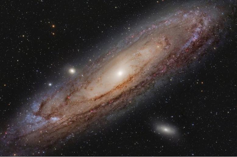
Devarshi Mandal SFJ3
In 1924, Edwin Powell Hubble (1889–1953) demonstrated that Andromeda (Messier 31 or M31), previously thought to be a nebula — an interstellar cloud of gas — was in fact a galaxy. This discovery overturned the prevailing belief that the Milky Way constituted the entirety of the Universe. Hubble’s work dismantled the notion that what we now recognise as galaxies were merely nebulae within the Milky Way, revealing an extremely vast Universe populated by countless galaxies beyond our own (Roy, 2024).
Returning a few years to April 1920, the historic Great Debate, hosted by the Natural History Museum in Washington DC, served as a stage for competing theories on the scale of the Universe. This occurred at a meeting
of the American Astronomical Society. Also known as the Shapley-Curtis debate, at the heart of the debate were astronomers Harlow Shapley, and Heber Doust Curtis. Both men had immensely differing ideas, with Shapley upholding the belief that what had been identified as “spiral nebulae” were just that, gas clouds. The Milky Way and the Universe were indistinguishable and not defined as separate entities. In this model, the Sun was placed far from the Milky Way’s centre. Meanwhile, Curtis argued for the idea of “island universes” (i.e. galaxies) as the true nature of these “spiral nebulae”, including Andromeda. The Universe was rather constructed of many galaxies, akin to the Milky Way. However, Curtis located the Sun as being close to the galaxy’s centre (American Physical Society, n.d.).
At the time, this debate would ultimately end in a stalemate, remaining unresolved due to a lack of conclusive observational evidence until four years later with Hubble’s work in 1924. His discovery further relied on the earlier work of Henrietta Swan Leavitt (1868 - 1921).
Leavitt concerned herself with Cepheid variables — a type of variable star that pulsates radially, changing in both diameter and temperature and exhibiting a stable period and amplitude of brightness variation. Leavitt’s work enabled the determination of distances to such stars.
During her work at the Harvard College Observatory in the first decade of the 1900s, Leavitt studied the Magellanic Clouds — the Small Magellanic Cloud (SMC) and the Large Magellanic Cloud (LMC) — which are now recognised as two dwarf galaxies, and satellites of the Milky Way. In this time, she compiled a list of 1,777 periodic variables, classifying 47 of them as Cepheid variables located in the Magellanic Clouds. By observing these stars, she noted that those with longer periods were brighter than those with shorter periods. Additionally, she deduced that since these variables shared the common location of the Magellanic Clouds, they were approximately the same relative distance from Earth. This led her to infer that any differences in their apparent magnitude — how bright a star appears from Earth — must result from variations in absolute magnitude, which is the intrinsic brightness of a star if viewed from a standard distance of 10 parsecs. A parsec is defined as the distance at which Earth’s orbital radius subtends an angle of one arcsecond (1/3600 of a degree), approximately equal to 3.26 light years. Therefore, the link between period and brightness was not a coincidence. Plotting her results for the SMC and LMC, she noticed distinct relationships between brightness and period (Australia Telescope National Facility, n.d.).
These relationships, which link the luminosity of pulsating variable stars to their pulsation periods, are known as period-luminosity relations. For Classical Cepheids, this is specifically referred to as the Leavitt Law. It is a proportionality relationship between absolute magnitude and the logarithm of time period.
Leavitt’s Law enables the calculation of a Cepheid’s absolute magnitude (M) from its measured period (P [days]), with constants (a, b), which would have been determined by calibration of the relationship:
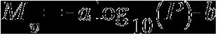
Equation 1: General PL relation for Cepheids.
Equation 2: Calibrated PL relation from Groenewegen for the V-band (visible light).
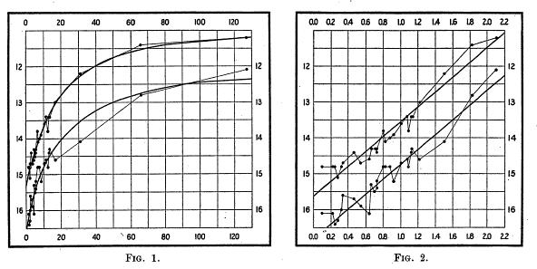
Figure 1: Plots of data concerning several Classical Cepheids. Left: Leavitt’s plot of magnitude against period. Right: Leavitt’s plot of magnitude against the logarithm of period (Foxell, 2019).
The constant values in equation 2 come from the calibration efforts of Groenewegen, using data from the GAIA DR2 parallax measurements to refine the period-luminosity relationship for Cepheids, although the values used by Hubble were much less refined.
Once the period-luminosity relation is calibrated — making absolute magnitude calculable from period — these stars can serve as standard candles. Standard candles are astronomical objects with known absolute magnitude, which can be used to determine the distance of the object using the distance-modulus formula. Cepheid variables were the first standard candles used in astronomy. The distance-modulus formula requires a known apparent magnitude (m), absolute magnitude (M), and distance (d) (Durham University, 2020):

Equation 3: Distance-modulus formula.
This discovery by Leavitt allowed Hubble to determine the distance of Cepheids located within the Andromeda “spiral nebula”. Hubble’s proof that Andromeda lay outside the Milky Way, as its own “island universe” relied on proving that these distances were greater than those to the estimated edge of the Milky Way (Resnick, 2016).
Hubble, working at the Mount Wilson Observatory in California, was operating the 100-inch Hooker Telescope, the largest telescope in the world at the time. He utilised the instrument to examine the “spiral nebulae”, appearing as cloud-like patches of light. Hubble stated that “the 100-inch reflector partially resolved several of the nearest neighbouring spiral nebulae into clusters of stars.” Among these nebulae that Hubble photographed was the then “Andromeda Nebula” (NASA, n.d.).
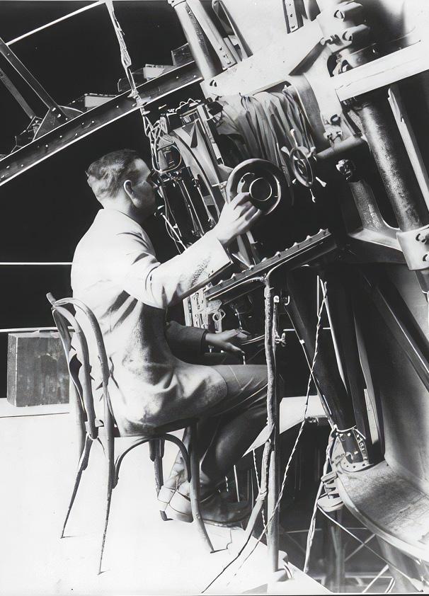
resolved his first Cepheid variable, designated Hubble variable number one (V1), located in the galaxy’s outer regions. Initially misidentified as a nova, subsequent photographs revealed variations in brightness over time, prompting its reclassification. By tracking these changes, Hubble determined the apparent magnitude of V1, using this photometric data to create a light curve. This allowed him to ascertain both the average apparent magnitude and period of V1. Applying the Leavitt Law, he calculated the variable’s absolute magnitude, and through the distance-modulus formula, he used the apparent and absolute magnitudes of V1 — a standard candle — to compute its distance from Earth (Carnegie Science, n.d.) (HEASARC, 2017).
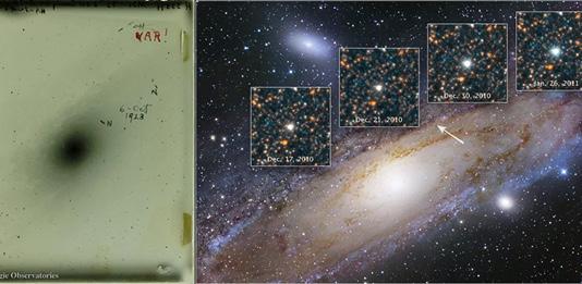
Following these calculations, it was clear: V1 and therefore Andromeda lay far beyond the bounds of the Milky Way. Hubble discovered that Cepheid variable stars in the Andromeda Galaxy were significantly more distant than those in the Milky Way. This discrepancy in distance led him to conclude that the “Andromeda Nebula” was, in fact, a separate galaxy. Employing this method, Hubble investigated other “spiral nebulae” throughout the universe, ultimately determining that millions of galaxies existed beyond our own (NASA, n.d.).
In 1923, while studying the Andromeda Galaxy, Hubble discerned individual stars within it. On the night of October 5-6, he captured a photographic plate, identified as Hooker plate 335 by Hubble (H335H), on which he
So, succeeding the 1924 discovery, Hubble presented his results in January 1925, at yet another meeting of the American Astronomical Society, settling the Great Debate, proving both Shapley and Curtis wrong, and shifting humanity’s perspective on the Universe (Resnick, 2016).
The Nobel Prize in Chemistry 2024 was awarded to David Baker, Demis Hassabis, and John M. Jumper for their groundbreaking work in protein design and prediction. Baker pioneered computational methods to design proteins
with specific functions, revolutionising drug discovery and biotechnology. Hassabis and Jumper developed AI-based techniques to predict protein structures with remarkable accuracy, a breakthrough that has transformed biology and accelerated medical research..

The Nobel Prize in Physics 2024 was awarded to John Hopfield and Geoffrey Hinton for their pioneering contributions to machine learning with artificial neural networks. Hopfield developed a model that mimics the brain’s ability to store and retrieve memories, providing a foundational framework for neural networks. Hinton’s invention of the backpropagation algorithm enabled machines to automatically learn patterns from data, a breakthrough that underpins today’s large-scale AI systems.
The evolution of astronomical discoveries
Advait Tripathi 10M1
Crane, L. (2019). First ever real image of a black hole revealed. Retrieved February 3, 2024, from New Scientist: https://www.newscientist.com/ article/2199330-first-ever-real-image-of-a-black-hole-revealed/ European Space Agency. (2019). A History of Astrometry. Retrieved December 5, 2023, from https://sci.esa.int/web/gaia/-/53196-the-oldestsky-maps
Finocchiaro, M. A. (2016). 400 Years Ago the Catholic Church Prohibited Copernicanism. Retrieved December 5, 2023, from https://origins.osu. edu/milestones/february-2016-400-years-ago-catholic-church-prohibitedcopernicanism
Gregersen, E. (n.d.). Understanding Kepler’s Laws of Planetary Motion. Retrieved December 5, 2023, from Britannica: https://www.britannica. com/story/understanding-keplers-laws-of-planetary-motion NASA. (2023). Edwin Hubble. Retrieved December 5, 2023, from https:// science.nasa.gov/people/edwin-hubble/ NASA. (2023). Hubble Observatory. Retrieved February 3, 2024, from https://science.nasa.gov/mission/hubble/observatory/ Royal Museums Greenwich. (n.d.). Galileo and astronomy. Retrieved December 5, 2023, from https://www.rmg.co.uk/stories/topics/what-did-galileo-discover
Tillman, N. T., & Dobrijevic, D. (2023). Black holes: Everything you need to know. Retrieved December 5, 2023, from https://www.space. com/15421-black-holes-facts-formation-discovery-sdcmp.html Westman, R. S. (2023). Nicolaus Copernicus. Retrieved December 5, 2023, from Britannica: https://www.britannica.com/biography/Nicolaus-Copernicus
E pur si muove – Galileo’s discoveries and how they changed the World Bibliography
Adam Smith SFH2
AHUJA, A. (2016). Echoes of Galileo in the populist retreat from reason. Financial Times. Retrieved 05 25, 2024, from https://www.ft.com/content/ f1a11abe-bb9a-11e6-8b45-b8b81dd5d080
Austrailia Telescope National Facility. (2015). Galileo and the Telescope. Retrieved 06 08, 2024, from https://www.atnf.csiro.au/outreach/education/senior/astrophysics/galileo.html
Del Soldato, E. (2023). Natural Philosophy in the Renaissance. In E. N. (eds.), The Stanford Encyclopedia of Philosophy (Fall 2023 Edition). Retrieved 05 25, 2024, from https://plato.stanford.edu/archives/fall2023/ entries/natphil-ren/
Kuhn, T. S. (1985). The Copernican Revolution. Harvard University Press. Retrieved 05 25, 2024, from https://fpa2014.wordpress.com/wp-content/ uploads/2014/01/kuhn-thomas-s-the-copernican-revolution.pdf NASA. (2011). Galileo’s Phases of Venus and Other Planets. Retrieved 05 25, 2024, from https://science.nasa.gov/resource/galileos-phases-of-venus-and-other-planets/ NASA. (2024, 02). Ganymede: Facts. Retrieved 06 08, 2024, from https:// science.nasa.gov/jupiter/moons/ganymede/facts/
Alan Hodgkin, Andrew Huxley, John Eccles and how they changed the way we understand our brains
Joshua Man SFS3
Anon., 2017. Alan Hodgkin - Facts - Nobel Prize. [Online]
Available at: https://www.nobelprize.org/prizes/medicine/1963/hodgkin/ facts/
[Accessed 5 1 2024].
Curtis, R., 2015. Sir John Eccles. [Online]
Available at: https://jcsmr.anu.edu.au/about/honour-roll/sir-john-eccles#:~:text=Sir%20John%20Eccles%2C%20Foundation%20Professor,carried%20out%20in%20the%20School. [Accessed 5 1 2024].
Haberman, F. W., 1972. In: Nobel Lectures. s.l.:Elsevier Publishing Company, p. 496.
Häusser, M., 2000. The Hodgkin-Huxley theory of the action potential. [Online]
Available at: https://www.nature.com/articles/nn1100_1165 [Accessed 5 1 2024].
National Center for Biotechnology Information, 2004. Serotonin. [Online]
Available at: https://pubchem.ncbi.nlm.nih.gov/compound/Serotonin [Accessed 17 June 2024].
Okinawa Institute of Science and Technology, 2020. Diagram of synaptic transmission. [Online]
Available at: https://www.oist.jp/image/diagram-synaptic-transmission [Accessed 17 June 2024].
Petousakis, A. P., 2022. The impact of Hodgkin-Huxley models on dendritic research.
Schwiening, C. J., 2012. A brief historical perspective: Hodgkin and Huxley. [Online]
Available at: https://www.ncbi.nlm.nih.gov/pmc/articles/PMC3424716/ [Accessed 5 1 2024].
James Webb Space Telescope
Sahil Bhutani 8S2
Fisher, A., 2022. NASA’s Webb Takes Its First-Ever Direct Image of Distant World. [Online]
Available at: https://blogs.nasa.gov/webb/2022/09/01/nasas-webb-takesits-first-ever-direct-image-of-distant-world/ [Accessed 1 April 2024].
NASA, 2016. Webb Space Telescope. [Online] Available at: https:// webbtelescope.org/contents/media/images/4181-Image#:~:text=Caption,(nearly%2050%20square%20feet). [Accessed 2024].
NASA, 2021. Fine Guiding Sensor. [Online] Available at: https://webb. nasa.gov/content/observatory/instruments/fgs.html [Accessed 13 January 2024].
NASA, 2021. MIRI- James Webb Space Telescope. [Online] Available at: https://webb.nasa.gov/content/observatory/instruments/miri.html [Accessed 13 January 2024].
NASA, 2021. Mirrors- Webb. [Online] Available at: https://webb.nasa.gov/ content/observatory/ote/mirrors/index.html [Accessed 13 January 2024].
NASA, 2021. NIRcam. [Online] Available at: https://webb.nasa.gov/content/observatory/instruments/ nircam.html [Accessed 13 January 2024].
NASA, 2021. NIRspec. [Online] Available at: https://webb.nasa.gov/ content/observatory/instruments/nirspec.html [Accessed 13 January 2024].
NASA, 2023. NASA James Webb Space Telescope - NIRspec. [Online] Available at: https://webb.nasa.gov/content/observatory/instruments/ nirspec.html [Accessed 4 January 2024].
Northrop Grumman, 2023. James Webb Space Telescope. [Online] Available at: https://www.northropgrumman.com/space/james-webbspace-telescope [Accessed 13 January 2024].
Phys org, 2016. Phys org. [Online] Available at: https://phys.org/ news/2022-03-nasa-james-webb-space-telescope.html [Accessed 2024].
Royal Museums Greenwich, 2021. Royal Museum Greenwich James Webb Space Telescope. [Online] [Accessed 2024].
Science Notes, 2024. What is a Micron?. [Online] Available at: https://sciencenotes.org/what-is-a-micron-definition-and-examples/ [Accessed 13 January 2024]. space.com, 2022. JWST: 12 big discoveries. [Online] Available at: https://www.space.com/james-webb-space-telescope-12-amazing-discoveries [Accessed 13 January 2024].
Could new advancements in technology finally make a Mars Base possible?
Richard Zhou 11R1
Anon., n.d. Mars: Facts - NASA Science. [Online] Available at: https://science.nasa.gov/mars/facts/ [Accessed 2023]. Grady, M., 2022. How to grow plants on the moon. [Online] Available at: https://phys.org/news/2022-05-moon.html [Accessed 2023].
Hoffman, J. A., 2022. Mars Oxygen ISRU Experiment (MOXIE)—Preparing for human Mars exploration. Mars Oxygen ISRU Experiment (MOXIE)— Preparing for human Mars exploration, 31 August, pp. 1-6.
Keeter, B., 2022. Scientists Grow Plants in Lunar Soil. [Online]
Available at: https://www.nasa.gov/humans-in-space/scientists-growplants-in-lunar-soil/ [Accessed 2023].
Learn, J. R., 2021. Colonizing Mars could speed up human evolution. [Online]
Available at: https://astronomy.com/news/2021/10/colonizing-mars-could-speed-up-human-evolution. [Accessed 2023].
Tomaswick, A., 2020. Astronauts and explorers on Mars could eat labgrown steaks. [Online]
Available at: https://www.universetoday.com/148702/astronauts-and-explorers-on-mars-could-eat-lab-grown-steaks/ [Accessed 2023].
Zubrin, R., From Ad Astra July/August 1996. The case for colonizing Mars, by Robert Zubrin. [Online]
Available at: https://space.nss.org/the-case-for-colonizing-mars-by-robertzubrin/ [Accessed 2023].
Cryptography Unravelled
Isaac Collis 10R2
Aditya, J. & Rao, S., 2005. Quantum Cryptography. [Online]
Available at: https://cs.stanford.edu/people/adityaj/QuantumCryptography.pdf [Accessed March 2024].
Coffey, N., 2021. RSA Key Lengths. [Online]
Available at: https://www.javamex.com/tutorials/cryptography/rsa_key_ length.shtml [Accessed March 2024].
Fruhlinger, J., 2022. What is cryptography? How algorithms keep information secret and safe. [Online]
Available at: https://www.csoonline.com/article/569921/what-is-cryptography-how-algorithms-keep-information-secret-and-safe.html [Accessed March 2024].
Kumar, A., 2024. Caeser Cipher in Cryptography. [Online]
Available at: https://www.geeksforgeeks.org/caesar-cipher-in-cryptography/ [Accessed March 2024].
Singh, S., 2000. The Code Book. New York: Anchor Books. Subramanian, V., 2021. Quantum and the Future of Cryptography. [Online] Available at: www.nationaldefensemagazine.org/articles/2021/12/27/ quantum-and-the-future-of-cryptography [Accessed March 2024].
The GPS Phalgun Deevanapalli SFR3 General:
Manning, C. (2023). GPS. [online] NASA. Available at: https://www.nasa. gov/directorates/somd/space-communications-navigation-program/gps/ (Accessed: 14 January 2024).
Singh, I. (2023) Who invented the GPS? people behind the global positioning system, Geoawesomeness. Available at: https://geoawesomeness. com/eo-hub/who-invented-the-gps/ (Accessed: 14 January 2024). Hardy, J. (2023) Who invented GPS? powerful Minds behind the history of GPS, History Cooperative. Available at: https://historycooperative.org/ who-invented-gps/ (Accessed: 14 January 2024).
GPS.GOV (2019). GPS: The Global Positioning System. [online] Gps.gov. Available at: https://www.gps.gov/ (Accessed: 14 January 2024). Eoportal.org. (2024). TIMATION: GPS Predecessor Program - eoPortal. [online] Available at: https://www.eoportal.org/other-space-activities/timation (Accessed 8 Sep. 2024).
Psu.edu. (2023). Welcome to GEOG 862 - GPS and GNSS for Geospatial Professionals | GEOG 862: GPS and GNSS for Geospatial Professionals. [online] Available at: https://www.e-education.psu.edu/geog862/ (Accessed 14 Jan. 2024).
GPS Directorate & Missile Systems Center (2019) NAVSTAR GPS Space Segment/Navigation User Segment Interfaces (IS-GPS-200)’ (Accessed: 14 January 2024).
Figure Sources: GPS.GOV (2019). GPS: The Global Positioning System. [online] Gps.gov. Available at: https://www.gps.gov/ (Accessed: 14 January 2024). Sfrcollege.edu.in. (2014). SFR | e-Content Development Program. [online] Available at: https://www.sfrcollege.edu.in/el-modules/Physics/GPS/segments.php (Accessed: 14 January 2024).
GPS Directorate & Missile Systems Center (2019) NAVSTAR GPS Space Segment/Navigation User Segment Interfaces (IS-GPS-200)’ (Accessed: 14 January 2024).
The untimely discovery of the World’s most important algorithm Oliver West SFM3
Arms Control Association, n.d. The Nuclear Testing Tally. [Online] Available at: https://www.armscontrol.org/factsheets/nucleartesttally
[Accessed 30 March 2024].
Cooley, J. W. & Tukey, J. W., 1965. An Algorithm for the Machine Calculation of Complex Fourier Series. Mathematics of Computation, 19(90), pp. 297-301.
Hardy, G. H., 1940. Mathematics in War-Time. Eureka, Issue 3, pp. 5-8.
Heideman, M. T., Johnson, D. H. & Burrus, C. S., 1985. Gauss and the History of the Fast Fourier Transform. Archive for History of Exact Sciences, 34(3), pp. 265-277.
Loan, C. v., 1992. Computational Frameworks for the Fast Fourier Transform. Philadelphia: SIAM Publications.
Rockmore, D. N., 2000. The FFT: An algorithm the whole family can use. Computing in Science & Engineering, Volume 2, pp. 60-64.
Rudnick, P., 1966. Note on the Calculation of Fourier Series. Mathematics of Computation, Volume 20, pp. 429-430.
Sanderson, G., 2018. But what is the Fourier Transform? A visual introduction. [Online]
Available at: https://www.3blue1brown.com/lessons/fourier-transforms [Accessed 30 March 2024].
Smith, S. W., 1997. Applications of the DFT. In: The Scientist and Engineer’s Guide to Digital Signal Processing. San Diego: California Technical Publishing, pp. 169-184.
U.S. Department of State, n.d. Treaty Banning Nuclear Weapon Tests in the Atmosphere, in Outer Space and Under Water. [Online] Available at: https://2009-2017.state.gov/t/isn/4797.htm [Accessed 30 March 2024].
Weisstein, E. W., n.d. Convolution Theorem. [Online] Available at: https://mathworld.wolfram.com/ConvolutionTheorem.html [Accessed 30 March 2024].
Weisstein, E. W., n.d. Fourier Series. [Online] Available at: https://mathworld.wolfram.com/FourierSeries.html [Accessed 30 March 2024].
Chirality and the Human Body - Zakariya Tanweer SFM3 Bogdan, M. et al., 2008. NIH. [Online] Available at: https://www.ncbi.nlm.nih.gov/pmc/articles/PMC5654212/ [Accessed 1st February 2024].
Christiante, L., 2012. Smart News. [Online] Available at: https://www.smithsonianmag.com/smart-news/thalidomide-manufacturer-finally-apologizes-for-birth-defects-survivors-say-its-no t-enough-24085623/ [Accessed 1st February 2024].
Crump, J., 2022. Sure Hire. [Online]
Available at: https://surehire.com/blog/2022/12/12/enantiomer-analysis-faqs/#:~:text=the%20positive%20test.-,Why%20is%20it%20essential%20to%20conduct%20an%20enantiomer%20analysis%3F,can%20 be%20far%20much%20dangerous
[Accessed 1st February 2024].
Egpat, 2019. eGPAT. [Online]
Available at: https://www.egpat.com/blog/list-amino-acids [Accessed 1st February 2024].
Greeves, N., 2023. ChemTube3D. [Online]
Available at: https://www.chemtube3d.com/sym-elementsplanes/ [Accessed 1st February 2024].
Hamosh, M., Bitman, J., L Wood, P. H. & Mehta, N. R., 1985. PubMed. [Online]
Available at: https://pubmed.ncbi.nlm.nih.gov/3880885/ [Accessed 1st February 2024].
Inaki, M., Liu, J. & Matsuno, K., 2016. National Library of Medicine. [Online]
Available at: https://www.ncbi.nlm.nih.gov/pmc/articles/PMC5104503/#:~:text=An%20item%20is%20chiral%20if,is%20essential%20 for%20their%20functions [Accessed 1st February 2024].
Inaki, M., Liu, J. & Matsuno, K., 2016. PubMed. [Online]
Available at: https://www.ncbi.nlm.nih.gov/pmc/articles/PMC5104503/#:~:text=An%20item%20is%20chiral%20if,is%20essential%20 for%20their%20functions [Accessed 1st February 2024].
Inokoshi, J. et al., 2009. Journal of Antibiotics. [Online]
Available at: https://www.nature.com/articles/ja20085 [Accessed 1st February 2024].
Klein, J., 2017. The New York Times. [Online]
Available at: https://www.nytimes.com/2017/06/14/science/louis-pasteur-chirality-chemistry.html#:~:text=When%20studying%20the%20
paratartaric%20acid,active%2C%20like%20the%20tartaric%20acid.
[Accessed 27th May 2024].
Liu, Z. & Rochfort, S., 2023. Science Direct. [Online]
Available at: https://www.sciencedirect.com/science/article/pii/ S2214799323000309
[Accessed 1st February 2024].
Malekinejad, H. & Rezabakhsh, A., 2015. NIH. [Online]
Available at: https://www.ncbi.nlm.nih.gov/pmc/articles/PMC4524299/#:~:text=The%20naturally%20occurring%20hormones%20 in,IGF%2D1%20(10)
[Accessed 1st February 2024].
Martin, C. & Freedman, S., 2014. Science Direct. [Online]
Available at: https://www.sciencedirect.com/topics/biochemistry-genetics-and-molecular-biology/lingual-lipase#:~:text=When%20a%20chiral%20 triacylglycerol%20with,glycerol%20and%20free%20fatty%20acid
[Accessed 1st February 2024].
McManaman, J. L., 2009. NIH. [Online]
Available at: https://www.ncbi.nlm.nih.gov/pmc/articles/PMC4459738/#:~:text=Milk%20lipids%20are%20derived%20by,cytoplasmic%20lipid%20droplets%20(CLDs).&text=CLDs%20are%20 generated%20at%20the%20endoplasmic%20reticulum%20by%20a%20 poorly%20understood%20mechanism
[Accessed 1st February 2024].
Nguyen, L. A., He, H. & Pham-Huy, C., 2006. Chiral Drugs: An Overview. International Journal of Biomedical Science, 2(2), pp. 85-100. Physics Open Lab, 2019. Physics Open Lab. [Online]
Available at: https://physicsopenlab.org/2019/08/20/optical-activity-chirality/
[Accessed 27th May 2024].
Pollegioni, L., 2019. IDAAR centre. [Online]
Available at: https://www.d-aminoacids.com/chirality/ [Accessed 1st February 2024].
Terauchi, Y. et al., 2018. Science Daily. [Online]
Available at: https://www.sciencedaily.com/releases/2018/10/181031093334.htm [Accessed 1st February 2024].
Willett, W. C. & Ludwig, D. S., 2021. The New England Journal of Medicine. [Online]
Available at: https://www.nejm.org/doi/full/10.1056/NEJMra1903547 [Accessed 25 Jun 2024].
Cosmic Microwave Background Radiation – how it was discovered and what it tells us
Hari Das 11C2
Chodos, A. (2002, July 1). June 1963: Discovery of the Cosmic Microwave Background. American Physical Society. Retrieved January 12, 2024, from https://www.aps.org/apsnews/2002/07/discovery-cosmic-microwave-background
The Nobel Foundation. (1978). Pyotr Kapitsa – Biographical - NobelPrize. org. Nobel Prize. Retrieved January 12, 2024, from https://www.nobelprize.org/prizes/physics/1978/kapitsa/biographical/ Tegmark, M., & Efstathiou, G. (1996, August 1). A method for subtracting foregrounds from multifrequency CMB sky maps. Oxford Academic. Retrieved January 12, 2024, from https://academic.oup.com/mnras/article/281/4/1297/1070061
Wall, M. (2014, May 20). Cosmic Anniversary: ‘Big Bang Echo’ Discovered 50 Years Ago Today. Space.com. Retrieved January 12, 2024, from https://www.space.com/25945-cosmic-microwave-background-discovery-50th-anniversary.html
Lineweaver, C. (2003, June 1). Inflation and the Cosmic Microwave Background. Research Gate. Retrieved January 12, 2024, from https://www.researchgate.net/publication/1931578_Inflation_and_the_ Cosmic_Microwave_Background
Could we ever create a plastic that decomposes?
Boran Sahin SFH1
Gallo, F. ,. F. C., 2018. Marine Litter Plastics and Microplastics and Their Toxic Chemicals Components: The Need for Urgent Preventive Measures. Environmental Sciences Europe, s.l.: s.n. Parker, L., 2018. National Geographic. [Online]
Available at: https://education.nationalgeographic.org/resource/whopping-91-percent-plastic-isnt-recycled/ [Accessed 27 May 2024].
Rannard, G., 2023. Oceans littered with 171 trillion plastic pieces. [Online]
Available at: https://www.bbc.co.uk/news/science-environment-64889284
Smith, M., 2018. Microplastics in Seafood and the implications for human health, s.l.: s.n.
Ripples in Spacetime: The Dance of Gravity
Aarav Shah 8J1
LIGO Lab. (n.d.-a). What are Gravitational Waves? | LIGO Lab | Caltech. LIGO Caltech. Retrieved October 8, 2024, from https://www.ligo.caltech. edu/page/what-are-gw
LIGO Lab. (n.d.-b). LIGO’s Interferometer | LIGO Lab | Caltech. LIGO Caltech. Retrieved October 8, 2024, from https://www.ligo.caltech.edu/ page/ligos-ifo
LIGO Lab. (n.d.-c). What is an Interferometer? | LIGO Lab | Caltech. LIGO Caltech. Retrieved October 8, 2024, from https://www.ligo.caltech.edu/ page/what-is-interferometer
LIGO Lab. (n.d.-d). Seismic Isolation | LIGO Lab | Caltech. LIGO Caltech. Retrieved October 8, 2024, from https://www.ligo.caltech.edu/page/ vibration-isolation
LIGO Lab. (n.d.-e). LIGO Technology | LIGO Lab | Caltech. LIGO Caltech. Retrieved October 8, 2024, from https://www.ligo.caltech.edu/page/ ligo-technology
LIGO Lab. (n.d.-f). Why Detect Them? | LIGO Lab | Caltech. LIGO Caltech. Retrieved October 8, 2024, from https://www.ligo.caltech.edu/page/whydetect-gw
Schilling, G. (2020, May 15). What is a pulsar? A complete guide to spinning neutron stars. BBC Sky at Night Magazine. Retrieved October 8, 2024, from https://www.skyatnightmagazine.com/space-science/what-is-apulsar-a-complete-guide-to-spinning-neutron-stars
Silver, A. (2017, October 3). Retrieved October 8, 2024, from https:// www.theregister.com/2017/10/03/gravitational_wave_detection_wins_nobel_prize_for_physics/
The 50th anniversary of the Expanded Programme on Immunisation (EPI)
Nathan Wolfson SFH2
Bill & Melinda Gates Foundation. (n.d.). Global immunization efforts have saved at least 154 million lives over the past 50 years. [online] Available at: https://www.gatesfoundation.org/ideas/media-center/press-releases/2024/04/global-immunization-fifty-years [Accessed 6 May 2024]. www.who.int. (n.d.). 50th anniversary of the Expanded Programme on Immunization (EPI). [online] Available at: https://www.who.int/news-room/ events/detail/2024/01/01/default-calendar/50th-anniversary-of-the-expanded-programme-on-immunization-(epi).
www.who.int. (n.d.). Celebrating 50 years of immunization progress: honouring achievements, embracing innovation, and envisioning the future. [online] Available at: https://www.who.int/news-room/events/ detail/2024/05/28/default-calendar/celebrating-50-years-of-immunization-progress-honouring-achievements-embracing-innovation-and-envisioning-the-future [Accessed 6 May 2024].
Vanderslott, S., Roser, M. and Dadonaite, B. (2022). Vaccination. [online] Our World in Data. Available at: https://ourworldindata.org/vaccination.
Leavitt, Hubble, and a larger Universe
Devarshi Mandal SFJ3
American Physical Society. (n.d.). This Month in Physics History. This Month in Physics History | American Physical Society. Retrieved September 1, 2024, from https://www.aps.org/archives/publications/apsnews/200004/ history.cfm
Australia Telescope National Facility. (n.d.). Cepheid Variable Stars & Distance Determination. Australia Telescope National Facility |. Retrieved September 1, 2024, from https://www.atnf.csiro.au/outreach/education/ senior/astrophysics/variable_cepheids.html
Carnegie Science. (n.d.). Hubble’s Famous M31 VAR! plate. Carnegie Science. Retrieved September 1, 2024, from https://carnegiescience.edu/ about/history/archives/plate-archives/m31var Durham University. (2020, June 17). The Period-Luminosity Relation of Cepheids. AstroLab. Retrieved September 1, 2024, from https://astrolab. awh.durham.ac.uk/cepheid.html
Foxell, E. (2019, March 8). Leavitt’s Standard Candles | astrobites. Astrobites. Retrieved September 1, 2024, from https://astrobites. org/2019/03/08/leavitt-variable-stars/ HEASARC. (2017, December 8). Cosmic Times. Cosmic Times. Retrieved September 1, 2024, from https://imagine.gsfc.nasa.gov/educators/programs/cosmictimes/online_edition/1929/andromeda.html
NASA. (n.d.). Edwin Hubble. NASA Science. Retrieved September 1, 2024, from https://science.nasa.gov/people/edwin-hubble/ Resnick, B. (2016, November 20). How Edwin Hubble discovered galaxies outside our own. Vox. Retrieved September 1, 2024, from https://www. vox.com/2016/11/20/13677046/edwin-hubble-andromeda-galaxy
Roy, J. R. (2024, March 21). Andromeda Galaxy at 100. Fifteen Eighty Four. Retrieved September 1, 2024, from https://cambridgeblog.org/2024/03/ andromeda-galaxy-at-100