Evaluating management regimes for European beech forests using dynamic programming
Juan Manuel Torres-Rojo 1 *, Frantisek Vilcko 2 and Klaus von Gadow 31 Centre for Research and Teaching of Economics. Ctra. México-Toluca, 3655. Col. Lomas de Santa Fé.
01210 México DF. 2 Burckhardt Institut. Geor-August-Universität. Büsgenwg, 5. 37077 Göttingen, Germany.
3 Department of Forest and Wood Science. University of Stellenbosch, South Africa and Burckhard Institut. Georg-August-Universität. Büsgenweg, 5. 37077 Göttingen, Germany
Abstract
Aim of study: This contribution describes a systematic search method for identifying optimum thinning regimes for beech forests ( Fagus sylvatica L.) by using a combination of optimization heuristics and a simple whole stand growth prediction model.
Area of study: Data to build the model come from standard and management forest inventories as well as yield tables from the Northern and Western part of Germany and from southern and central Denmark.
Material and methods: Growth projections are made from equations to project basal area and top height. The remaining stand variables are recovered from additional equations fitted from forest inventory data or acquired from other authors. Mortality is estimated through an algorithm based on the maximum density line. The optimization routine uses a two-state dynamic programming model. Thinning type is defined by the NG index, which describes the ratio of the proportion of removed trees and basal area with respect to the same proportion before thinning.
Main results : Growth equations fitted from inventory data show high goodness of fit with R 2 values larger than 0.85 and high significance levels for the parameter estimates. The mortality algorithm converges quickly providing mortality estimates within the expected range.
Research highlights: The combination of a simple growth and yield model within a Dynamic Programming framework in conjunction with NG values as indicators of thinning type yield good estimates of practical thinning schedules compared to thinning recommendations provided by diverse authors.
Key words : beech ( Fagus sylvatica L.); NG ratio; thinning optimization; growth and yield simulation; mortality.
Introduction
Despite its commercial and ecological importance, systematic attempts to generate and evaluate alternative treatment schedules for beech are surprisingly rare. Numerous proposals have been made and arguments presented in favor of particular treatment concepts for beech forests. One of the most comprehensive studies was presented by Schober (1972). Other detailed studies include those of Freist (1962), Altherr (1971), Wilhelm et al. (1999), and Klädtke (2002). These analyses are detailed and thorough, but to our knowledge, none of the proposals has been based on an exhaustive comparison of possible alternatives.
author: juanmanuel.torres@cide.edu
The objective of this paper is not to propose another specific silvicultural system, but to present a method for comparing treatment options for beech stands, based on the optimization technique known as Dynamic Programming ( DP ). This tool has been the most widely used technique to optimize silvicultural treatments. It was initially proposed by Arimizu (1959) and operationalized by Amidon & Akin (1968). Since then, the tool has been applied to a wide variety of evenaged management problems at stand level (Ritters et al. , 1982; Brodie & Haight, 1985).
Early scientists used a two descriptor DP model (usually volume and age) in order to cluster each state in the network (Brodie et al., 1978; Chen et al., 1980; Kilkki & Väisänen, 1970). A three descriptor model was first proposed by Brodie & Kao (1979). This model was the first one linked to an existing growth si-
mulator for Douglas-fir called DFIT, and the first attempt to simultaneously optimize thinning type, intensity and timing. Such a methodology of linking growth simulation models and dynamic programming optimization routines to optimize silvicultural treatments soon expanded, involving different species and objectives.
This paper describes an approach to identify optimal thinning schedules (thinning type, timing and intensity of a harvest event) with a three descriptor DP model linked to a simple whole stand growth model with no diameter distribution prediction capabilities. Thinning intensity is defined as the proportion of the basal area removed during a given harvest event and thinning type is described by using the NG ratio. NG is defined as the ratio of the number of trees removed ( N R ) to the number of trees before thinning ( N ), divided by the ratio of basal area removed ( G R ) to the basal area before thinning ( G ); the usual mathematical expression is:
be implemented. The third section shows comparative results including some sensitivities for different model parameters. The fourth section discusses some of the implementation problems as well as the precision of the assembled tool, while the final section provides some conclusions.
Material and methods
Growth model for beech
The first yield models for beech stands were developed more than 200 years ago. An example is the yield table published by Paulsen (1795). Improved yield tables were developed towards the end of the 19 th century and the beginning of the 20 th century on the basis of better growth data (Baur, 1881; Schwappach, 1890; Eberhard, 1902; Grundner, 1904; Wimmenauer, 1914; Wiedemann, 1931). More recently, Schober (1972) compiled a beech yield table for North-Western Germany, which is based on the work of Schwappach (1911) and Wiedemann (1931). Another beech yield table, which is mainly used in Eastern Germany was published by Dittmar et al . (1986).
NG values greater (smaller) than unity are associated with thinnings where the average size of the trees removed is smaller (greater) than the average size of the trees before thinning. This means that the NG value defines which tree sizes are more affected by the thinning on average. Such an information is crucial as the distribution of trees left after thinning will define future yields. Since there is a large number of feasible NG values when applying a given thinning intensity an additional optimization is also introduced to identify the best NG value ( i.e. the best combination of N R and G R ) associated with each thinning.
The objective of this study is to describe a systematic search method for identifying optimum silvicultural regimes for beech forests in Europe by using a combination of optimization heuristics and a rather simple growth prediction model assembled with data available from yield and stand tables as well standard inventory information. The paper is divided into four main sections. The next section briefly describes the growth and yield prediction model, data sources as well as presenting a summary of the traditional DP formulation for the stand level optimization problem. In the same section, the formulation to optimize NG ratios is discussed, as well as the technical problems that need to
Several single tree simulators for beech were developed during the 1990’s, e.g . the parametric models SILVA (Pretzsch & Kahn, 1998) and BWinPro (Nagel et al. , 2002), the non-parametric model MIBEA ( Hessenmöller , 2001) and the physiological model FAGUS (Hoffmann, 1995). The single tree growth models tend to show a rather high proportion of unexplained variation, and in some cases observed growth rates exceeded the potential rates of the growth models (Gadow and Heydecke, 2000). Consequently, it was decided to develop a whole stand growth model based on the volume prediction model developed by Franz et al. (1973), for this analysis. This model can be used to predict total stand volume (m 3 ha –1) after thinning, before thinning and even the thinning volume if appropriate variables are used. The model has the following form:
where H m is the mean height of the stand, which can be observed before thinning ( H m ) or for the removed stand ( H mR ) as it were the case; G is the basal area of the stand, which also can be observed before thinning ( G ), or for the removed ( G R ) stand (m 2 ha –1); d i corresponds to the i-th parameter.
For any prediction this model requires two basic variables at the predicted age and condition (before thinning or after thinning): mean height and basal area. For our model, the mean height of a stand (before thinning) is estimated from top height using an exponential model of the following form:
where H m is the mean height of the stand before thinning (m), and H 100 represents the mean height of the 100 tallest trees per ha (m).
The mean height of the removed stand is also estimated from top height corrected by the size of the thinned trees measured through the quadratic mean diameter. For this estimate we used the model:
where HmR is the mean height of the removed stand (m), H 100 is mean height of the 100 tallest trees per ha (m), and Dq R represents the quadratic mean diameter of the removed stand (cm). Greater precision in the estimate of H mR could be achieved by including an indicator of thinning type. However this information was not available from standard management inventories carried out in beech forests in northern Germany where we obtained the data.
These latter two models require an estimate of top height. For this component, the following dominant height model proposed by Sloboda (1971) was used:
where G 2 represents the basal area at age A 2 (m2 ha–1), G1 is basal area at age A1 (m2 ha–1), N2 represents the number of trees at age A2, while N1 is this number at age A1
Natural tree mortality cannot be estimated directly from yield tables, given that successive values for the number of trees presented in such tables might include thinned trees. Hence, a plausible estimate of tree mortality had to be derived. Such an estimate is based on the principle that predicted quadratic mean diameter recovered from predicted basal area and N2 (equation [5]) cannot exceed the maximum size allowed for a given density as defined by the maximum size-density relationship (Yoda et al. , 1963). The estimate of maximum density was derived from the model described by Döbbeler and Spellmann (2002), which has the following form: [6]
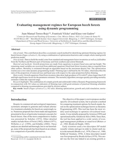
where N Gmax represents the maximum surviving trees per ha with quadratic mean diameter, Dq Gmax (cm). The parameter values for beech reported by the authors are p 0 =1.0829E–07, t 0 =8.3652, p 1 =1.5374, and t 1 = –1.7365. Given the maximum density (also known as the limiting relationship), the search for a feasible estimate for N 2 can be summarized by the following algorithm (see also Fig. 1):
where H 100 is the mean height of the 100 tallest trees per ha (m); SI represents site index (defined here as the top height at age 100, m); A 0 is the reference age (100 years), and A represents stand age.
Since mean height is driven by top height and this latter variable is uniquely defined by age (given that site index is considered constant within a given prediction interval), then mean height can be defined at any age given equations [2] and [4].
Another important element of the stand volume model (1) is basal area. Basal area growth is often estimated by using the path invariant algebraic difference form (also known as PID-type; Souter, 1986), which usually provides more accurate estimates when information is based on long term growth data, than a differential equation (DIF- type). The fitted model has the following form:
Step 1 Set the first guess of predicted number of trees ( N 2 * ) at A 2
N 2 *= N 1
Mortality=0
Step 2Computes G 2 using eq. [5];
Recover Dq 2 from N 2 * and G 2
Step 3If N 2 * ≤ N Gmax given Dq 2
Then G 2 is accepted; N 2 =N 2 *
Mortality= N 1 –N 2
Else
Correct the estimate for N 2 * ; Go to step 4
Step 4Estimate Dq*Gmax given N Gmax =N 2* from [6] Recover N*Gmax given from [6]
N 2 *= N * Gmax
Define initial conditions: G1, N1, A1, SI
Define projection Age (A2) Set guess of N2 = N2*= N1
Computes H100 = f (SI, A0, A2) Computes Hm = f (H100)
Computes G2 at A2 G2 = f (A1, A2, SI, N1, N2*)
Recover Dq2 from N2*and G2 Computes NGmax = f (Dq2)
N2* ≥ NGmax given Dq2
Yes
Guess for N2 is high
Set N2 = N2* and G2 is accepted as a valid projection
End Initiate Mortality simulation
Estimates V2
Mortality= N1 – N2
Computes H100 = f (SI, A0, A2) Computes Hm = f (H100) Computes V2 = f (Hm, G2)
Computes H100 = f (SI, A0, A1) Computes Hm = f (H100) Computes V1 = f (Hm, G) Yes
Another projection?
Simulate thinning?
Yes
Corrects N2*
Computes Dq*Gmax given NGmax Dq2 – Dq*Gmax Dq2 computes= 2
Recover NGmax given Dq* 2 (eq.[6])
Set N* 2 – NGmax
Define thinning parameters
Set type of thinning (NG)
Set removed basal area (GR)
Compute thinning volume
Recover DqR from GR and NR
Computes HmR = f (H100, DqR)
Computes VR = f (HmR, GR)
Figure 1. Flow chart for growth projection, thinning and mortality simulation.
In this algorithm N 2 * represents a guess (dummy) when searching for a feasible number of trees at the projection age (which means it does not violate the maximum density line constraint), while Dq 2* represents the quadratic mean diameter along the maximum density line given the guess N 2 *. Convergence is guaranteed as the search is over a closed interval. The binary search approach regularly converges after 6-7 iterations for an error ε =0.001 cm of Dq
Any projection starts from the definition of state variable values: site index ( SI ), initial Age ( A 1 ), initial basal area ( G 1 ), and initial number of trees ( N 1 ). H 100 , H m , and V 1 are recovered from equations [4], [2] and [1] respectively to describe the main variables at the initial age. Given initial values a projection age ( A 2 ) is defined and equation [5] is used to compute projected basal area ( G 2 ). Following the mortality algorithm an estimate of number of trees at the projection age ( N 2 ) is obtained and again, the basic information to describe the stand can be recovered. Fig. 1 shows a flow chart for a simple growth prediction including the search for a feasible estimate of mortality.
Data description
Data to fit the model come from different sources. Models (1), (2) were fitted using data from standard forest inventories available for Northern Germany at the Burckhardt Institut, Georg-August-Universität, Germany . The sample size is quite large ( n =7,420) since sample plots were used as sample units.
Model (3) was fitted using standard management inventories for thinned stands in Northern Germany. The sample size includes 1,328 observations from managed pure beech stands.
Model (4) was fitted using information from yield tables for North-western Germany (Schober, 1987) which includes estimates of top height. The sample for this fit included 198 observations. Finally, information to fit model (5) comes from German yield tables (Schober, 1987) and from very heavily thinned stands in Denmark (Skovsgaard & Mosing, 1996). To generate the basic information successive values of age, basal area and number of trees were generated. The sample size for this fit includes 340 observations. Given the source and variety of information the recommended growth projection interval is 10 years.
Optimization of timing and intensity of thinning
The standard Dynamic Programming formulation for simultaneously optimizing rotation age, thinning intensity, and thinning time as described by Brodie and Kao (1979) was used to find an optimal schedule of timing and intensity of thinning along the rotation. Such a formulation maximizes a value function (present net worth, land value or harvest volume) subject to constraints on state variables as follows:
where f N (y N ) is the objective function value of the sequence of thinning decisions in N management periods, yielding a final stand described by y N, which in an even aged management context corresponds to the stand after the final harvest; r n (t n ) represents the return (present net worth, land value or harvest volume) yielded at stage n when thinning decisions at state n (t n ) have been taken; y n is a vector describing the stand at stage n after thinning decision t n has been taken in a stand described by x n This vector describes the so called “residual stand”, “state descriptor” or “state variable”. The vector x n describes the stand at stage n after it grows from state y n -1 (before thinning). It is also referred to as the “initial stand vector” or “stand before thinning”. Vector t n describes feasible thinning decisions (intensity) at stage n transforming the stand x n into y n and generating a return r n (t n ) which is usually referred to as the vector of decisions variables and finally, the vector g n +1(y n ) represents the growth variables for a stand described by y n at stage n to stage n+ 1. It is usually referred as the transformation function (Paredes and Brodie, 1987) but in the present context is equivalent to the set of equations for growth prediction.
Optimizing the type of thinning
The control variable thinning (t n ), usually involves two or more descriptors according to the growth mo-
del characteristics. If only thinning intensity is to be evaluated, then just one descriptor is needed (usually basal area or volume). However, simulating the type of thinning requires at least two descriptors describing different stand characteristics before and after thinning. Usually these descriptors are basal area and number of trees, although other descriptors can be used if richer growth information and stand descriptors are available.
The NG ratio is a descriptor that combines these state variables as it provides information on the average size of the removed trees with regard to the original stand.
As stated above, NG values greater (smaller) than unity represent a thinning where the average size of the trees removed is smaller (greater) than the average size of the trees before thinning. It is true that for a given a removal intensity ( G R ), an NG value could be associated with combinations of small and large trees, nevertheless NG will describe the average size of the trees removed as compared to the average size of the trees before thinning (Staupendahl, 1999).
From this perspective the NG ratio opens the possibility for simulating different types of thinning for a given intensity without the need for predicting (or recovery of) the diameter distribution. The use of NG ratios becomes even more relevant for managing natural stands, where diameter distributions often are not unimodal but may be quite irregular (Gadow, 1992; Kassier, 1993; Staupendahl, 1999). In such circumstances, the NG ratio is a useful alternative to simple semantics for describing a management regime, as it is independent of the shape of the diameter distribution.
We define a “thinning of small trees” (“thinning of large trees”) to that thinning where the average size of the removed tree is smaller (greater) than the average size of the trees before the harvest. An extreme case of “thinning of small trees” (“thinning of large trees”) would be a thinning from below (thinning from above) where the smallest (greatest) trees are removed. We also define a mechanical thinning to be one where the average size of the removed trees is equal to the average size of the trees before thinning.
For a given removal intensity many NG values greater (smaller) than unity would define a “thinning of small trees” (“thinning of large trees”) each one of these values will yield a residual stand and a removed stand that will generate different patterns of growth and thinning volume (yields) along the rotation . Hence there is a possibility to optimize NG values greater than unity (or between 0-1) that could be chosen at each state. Random selection over a feasible interval might be an alternative to find the best NG ratio. Observe that if such interval is not defined appropriately, one might be ending selecting an NG ratio representing an impossible combination of trees to be thinned or an undesirable type of thinning. Nevertheless such bounds are easy to find just from a redefinition of the NG ratio as follows1:
where k is a constant, Dq represents the quadratic mean diameter before thinning while Dq R is the quadratic mean diameter of the removed trees. For a thinning from small trees, NG must be greater than one, and somehow must have an upper bound ( UB ) defined by physical conditions (state variables) as follows: [9]
How close NG is to unity depends on the variance of the diameter distribution. The smaller the variance, the closer the NG ratio can approximate to unity. The upper bound ( UB ) can be obtained with a simple analysis of the NG relationship. Considering [8] and the fact that N must always be greater than N R , we can state:
Using similar reasoning, it can be found that the bounds for a thinning from above are:
1 In some countries the ratio where is the mean diameter of the removed trees and is the mean diameter of the trees before thinning is more frequently used than the NG ratio. Both ratios are linked through the following relationship:
which represent the bounds to search for feasible NG values 2 . Since there are many possible paths with different NG values at each state, the DP model should incorporate NG as another state descriptor of the network. However, because of dimensionality this would substantially increase the size of the problem. Another approach is to optimize NG at each state by using the PATH algorithm (Paredes and Brodie, 1987). To implement the algorithm, consider Fig. 2; a two-stage traditional DP network (under the neighborhood approach). Assume the initial condition y n–1, which represents a stand that is projected to the second stage to reach state conditions x n . At this stage, three thinnings of the same intensity (same removed basal area G R ) and type ( NG within certain bounds) are simulated, each one with different residual numbers of trees per hectare ( N R ), which yield different NG ratios. Observe that if a diameter distribution were available, the thinning intensity defines a unique N R as trees are thinned from one of the tails (for a thinning from below or from above) and therefore a unique NG could be obtained. However, without such a distribution, thinning intensity can be generated by different com-
binations of tree size, hence it becomes necessary to approximate the NG ratio that will maximize the total value function along the rotation. Such an optimization is made in a nested network with the use of the PATH algorithm, projecting each state at stage n (representing resulting NG ratios) to the next stage ( n+ 1) and valuing the whole projection (see Fig. 2). The selected NG ratio will be the one with the highest total return and will be the base to continue the dynamic optimization along the rotation.
The DP network and the growth model were assembled within a computer program (DPFAGUS Ver 1.0) written in FORTRAN, where optimal thinning schedules can be obtained under different initial stand conditions, economic information (product price and input costs), residual basal area constraints, thinning types, and objective function formulations.
The network is built on a grid where each cell represents a feasible combination of state variables ( G and N ) as shown in Fig. 2. The size of the cell defines an interval of values where the state variable could lie after a projections or a thinning (neighborhood approach). This last feature is important as the precision of the optimization will depend on the size of the cells in the grid. The computer program allows for different projection intervals (growth projection periods) and different sizes of the grid for state variables. Given the kind of information used to build the models it is recommended to use 10 years intervals.
Results
Growth equations
Parameters from growth equations were estimated through least squares procedures. Table 1 shows the estimate values as well as the standard error for the estimates (in parenthesis) and the adjusted R 2 as goodness of fit criterion.
In all cases the fittings are very good given the values of R 2. The main equation, the basal area projection (equation [5]) is the one with the lowest R 2 . No data were left for a validation test for this model, however, residuals showed no signs of heteroskedasticity,
2 For a given NG , the ratio G / GR could be such a big number if G R is small enough. Feasible values for N R were define not be smaller than d –3* Var ( d ) (confidence interval for d ) where Var ( d )= Dq 2 – d 2 and the estimate of d can be obtained from regressing d as a function of age from stand or yield table data. Solution beyond the range are usually ignored along the optimization as th ey involve low value trees.
*Values in parenthesis show standard errors.
autocorrelation (AR(1) was the only one tested) or nonlinearities.
Optimization results
Standard conditions
The DP network was validated with different values for the grid size defined by the state variables. Widths less than 1.5 m 2 basal area and less than 15 trees per hectare yielded very similar objective function values. The grid size for the NG values was also evaluated, keeping in mind that this grid is stage dependent (old ages require a finer grid). For this grid, NG intervals less than 0.05 did not yield any significant differences. Nevertheless, the NG grid interval was fixed at 0.01 for the simulations. The network was set to these upper bounds, assuming that solutions obtained by this size in both grids would approach those obtained from a continuous formulation of the problem.
Simulations were run to explore optimal paths for a range of residual basal areas, NG values and a speci-
fied projection period. For these simulations we assumed the following initial stand conditions: age=40 years, basal area=27 m 2 , number of trees per hectare=2,400 trees, and site index=35 meter, which represent average conditions for a young stand of the species growing on a good site within the area of its geographical distribution. The economic base line values were: zero interest rate, maximum time horizon of 130 years, thinning cost of € 9.40 m–3, thinning entry cost of € 80.00 ha –1 , and no regeneration costs. In addition, differential prices per log diameter class were estimated by using the quadratic mean diameter of the removed trees as the mean diameter and an estimate of height and diameter distribution from a taper equation (Trincado and Gadow, 1996). Log prices correspond to the standard classification in Lower Saxony, Germany. Table 2 shows the price-size gradient.
Effect of thinning type
Simulations were run assuming zero interest rate and constraining NG values to be greater than unity
(thinning of small trees), lower than unity (thinning of large trees) and without constraint (free) for a maximum time horizon of 130 years. Optimal thinning schedules under different thinning types, yielded the residual basal areas shown in Fig. 3.
Optimal residual basal areas are kept about the same levels along the rotation regardless the type of thinning (Fig. 3a). Thinning intensities are also similar, however, there is a huge difference with respect to the size of trees thinned along the rotation. In thinning of small trees, the average size of removed trees is small
until ages 80-90, a time period when thinnings are shifted to larger trees. For thinnings “of large trees”, the removed trees have about the same average size until age 90, when they are shifted to smaller size trees (NG values increase). For a free thinning type, the optimization suggests thinnings “of small trees” until age 80, and thinning “of large trees” thereafter (Fig. 3c).
The three simulations ( NG >1, NG <1 and NG free) yielded different objective function values (present net worth). Results show that the combination of thinning types along the rotation yields larger profits than
applying just one type of thinning. In this same order of ideas, thinnings of small trees applied during the first stages of the rotation reduce the profits measured in terms of present net worth values, in spite of the fact that residual basal areas are kept almost at the same order of magnitude along the rotation.
Effect of site index
The type and intensity of thinnings are silvicultural tools used to define the characteristics of the product at the end of rotation. Theory shows that in order to obtain large trees at the end of the rotation, heavy thinnings must be performed during early years. Optimal thinning schedules for beech show that valuable trees for sawn wood are obtained with heavy thinnings of medium to small size trees at the beginning of the rotation, and one or two heavy thinnings of large trees at the time when the maximum population growth rate is reached (Fig. 4). These results were obtained by assuming the base line characteristics, a free type of thinning and a zero interest rate.
Residual basal areas recommended by the optimization procedure are of the same order of magnitude, regardless the site index. Small variations depend on the fact that higher site indices allow higher growth rates and the possibility to thin more trees along the rotation, as well as to keep larger trees to the end. One interesting result from the simulation is the path of thinnings suggested by the optimization procedure. As it can be observed in Fig. 4b the higher the site index the faster the recommendation to thin more and larger trees along the rotation with the resulting higher profit. It can be observed that at higher site indices even more thinnings from above are recommended.
Effect of interest rate
It is well known that when maximizing any economic criterion, an increasing interest rate reduces the rotation age and requires heavier thinnings at the beginning of the rotation. In the case of beech simulations with the standard conditions showed that the optimal rotation age with no interest rate is approximately 130 years. With interest rates ranging between 1 and 4 percent, the optimum rotation age reduces to 120 years. Using interest rates between 5 and 7 percent, the optimum rotation is further reduced to 115 years. From 8-12 percent interest rate the optimum rotation age is only 110 years. Evidently, the greater the interest rate, the heavier should be the thinnings at the beginning of the rotation period. Fig. 5 presents the optimum residual basal areas for different interest rates under the assumed initial conditions. Observe that high interest rates require heavy thinning at ages 50-60 years just when commercial volumes are barely available (NG values close to 1). Then a basal area around 26 m2 ha–1 is maintained until the end of the rotation, while the basal area is kept at higher levels (Fig. 5a) for longer rotations. The pattern of thinning types along the rotation also changes with different interest rates. While there is a smooth transition between thinnings of small trees to thinnings of large trees, when no interest rate is considered, higher interest rates require heavier thinnings of small trees at the beginning. When the interest rate is extremely high, those heavy thinnings are converted into thinnings of large trees.
Discussion
Our discussion will deal with four points: the growth projection approach, the optimization approach, the
use of NG to identify the type of thinning and the optimization tool.
As referred to in the introduction ,there is a lot of information on growth of beech under different conditions. What we wanted to illustrate is how we can use this information available in common management inventories, yield and stand tables as well as specific references to assemble a set of equations with a relatively high degree of precision to predict beech growth. Beyond the goodness of fit of the models proposed we checked how predictions are made with the whole set of equations. Few data are available to compare those predictions but for the range of information available on yield tables with heavy thinnings the projections are very close compared to those in the tables. There are some deficiencies of the growth projection approach, among them:
i)Mortality is not precisely defined though a deterministic model, on the contrary is “guessed” under the assumption that the basal area projection is good and that the maximum density line constraints the average size given a specific density. The convergence of the algorithm is guaranteed, however it just offers a linear approximation to a process that is nonlinear. In addition, since the mortality is referred to the maximum density line, high densities are always allowed.
ii)The model to estimate the size of removed trees could be improved if additional information such as thinning type, variance of the diameter distribution before thinning or at least a before thinning would be available. The current estimate might yield biased estimates with perhaps not such big effects for valuation given that high logs have always a lower value.
The optimization approach is a standard Dynamic Programming formulation of a thinning-rotation optimization problem widely referred to in the forestry li-
terature. The additional feature is that the approach combines the traditional optimization through all stages with the PATH algorithm introduced to optimize NG . This feature presents an opportunity to introduce another decision element in the control variable t which is not to be reflected in the formulation by extending the optimization network. If concavity of the production functions holds, as expected, the approach should not have problems. However, real conditions might allow certain convexities at some stages of growth which are not captured by the growth model and could question the optimization results. We did not have a chance to detect those convexities but we assume they could occur.
The use of NG seems new in our optimization approach. We introduced it because we did not have a diameter prediction model available, beyond the problems related with the diameter distributions of the beech forests. It is true that NG just gives a rough idea of the average size of the removed trees compared with the size of the trees before thinning. This is enough to compare the thinning schedules available in yield tables and references against our results. One challenge in the optimization was to identify the searching interval to optimize NG , however as described above, rough upper and lower bounds could be defined. These bounds might still yield impossible combinations of tree sizes to be thinned (very thin or extremely large trees). Some strategies to delete those combinations were implemented, among them, checking the size of removed trees against a confidence interval of a taper equation, or an even simpler one, checking the size of the average removed tree against predicted values of regressions between minimum or maximum diameters against age. However, those additional limits were not necessary since we learned that those atypical or im-
possible combinations of removed trees yield low values for the thinning and for the future yield so they are eliminated along the optimization approach.
The assembled tool seems to work very well for a species as complicated to manage as beech. Traditional variables used to manage forests systems as rotation, density and site index are not sufficient in the case of European beech where there are many additional aspects to consider (like price-size gradients; very specific silvicultural options; beech often grows in mixture with other species). Such a complexity and the fact that beech rarely appears in pure stands seem to be reasons why the dynamic programming approach has never really been successfully applied in beech forests. The optimization tool we present in this paper combines a simple growth model with a Dynamic Programming optimization routine. Obviously the tool is as precise as the precision of the growth projection model. However, beyond the precision on growth projections and the optimization of thinnings through NG ratios, the simple tool provides comparable results with respect to recommendations made by experienced practitioners. For example the three schedules shown in Fig. 3 b) are very similar in trend to the ones suggested by Freist (1962) and Altherr (1971), though the residual basal areas obtained through optimization are slightly higher than the ones reported by these authors. The discrepancy might be explained by the fact that the growth model allows for larger stand densities, since stocking is taken to the limit of the density line. Another difference between the schedules recommended by Freist and Altherr and those obtained from the optimization is that, according to these authors, the first peak of residual basal area is at 50 years, and according to the optimized schedule it is around 60 years, which confirms that the growth prediction model allows for higher densities and growth rates.
Conclusions
The purpose of this paper was to present a systematic search method for identifying optimum silvicultural regimes for beech forests in Europe by using a combination of optimization heuristics and a simple growth prediction model assembled with data available from yield tables as well standard inventory information. To the best of our knowledge, this is the first application of Dynamic Programming to this particular species.
Although a huge database of long term growth information for European beech does exists, very simple assumptions have to be made to build a growth prediction model which is suitable for standard economic analysis tools, such as Dynamic Programming. The existence of an empirical data base is irreplaceable as more sophisticated and specific growth predictions are required and there are indications that in time this deficiency will be overcome (Álvarez-González et al. , 2009; Zhang et al. , 2009). The use of NG ratios to define the thinning type proved to be useful within this particular optimization framework. It not only provides a practical tool for defining the type of thinning to be implemented, but also does not carry the disadvantages of traditional diameter distribution prediction (or recovery) approaches, since it is independent of the shape of the diameter distribution. Once improved harvest event models have been developed, these can be adapted to any economic and stand condition to define practical thinning schedules. As shown in this paper, optimization results yielded thinning schedules similar to those suggested by several authors. Further development is warranted to create a sound scientific basis for practical silvicultural recommendations.
Acknowledgements
We thank the German Academic Exchange Service (DAAD) for founding the reasearch stay of the first author at the Institut für Waldinventur und Waldwachstum (Göttingen, Germany) where this reasearch was developed.
References
Altherr E, 1971. Alternatives to producing large dimensional beech logs. Report for the 15 th meeting of the Forestry Union of Baden-Württemberg. Forstverein. pp:123-127.
Álvarez-González JG, Zingg A, Gadow Kv, 2009. Estimating Growth in Beech Forests – A study based on longterm experiments in Switzerland. Annals of Forest Science 67: 307.
Amidon EL, Akin GS, 1968. Dynamic programming to determine optimal levels of growing stock. Forest Science 14: 287-291.
Arimizu T, 1959. Dynamic programming in forestry. J of Japan Forest Society 41: 448-458.
Baur F, 1881. About thinnings and thinning trials. In: Das forstliche Versuchswesen (Ganhofer A, ed). Vol 1. Commission der B. Schmid’schen Buchhandlung (A. Manz).
Brodie JD, Adams DM, Kao C, 1978. Analysis of economic impacts on thinning and rotation for Douglas-fir using dynamic programming. Forest Science 24: 513-522.
Brodie JD, Haight RG, 1985. Optimization of silvicultural investment for several types of stand projection system. Canadian J of Forestry Research 15: 188-191.
Brodie JD, Kao C, 1979. Optimizing thinning in Douglas fir with three-descriptor dynamic programming to account for accelerated diameter growth. Forest Science 25: 665-672.
Chen CM, Rose DW, Leary RA, 1980. Derivation of optimal stand density over time-a discrete stage, continuous state dynamic programming solution. Forest Science 26: 217-227.
Dittmar O, Knapp E, Lembcke G, 1986. GDR Yield Table for beech 1983. IFE-Berichte.
Döbbeler H, Spelmann H, 2002. Methodological approach to simulate and evaluate silvicultural treatments under climate change. Forstw. Cbl 121(Supplement 1): 52-69.
Eberhard J, 1902. Tables for estimating site quality and yields based on mean height for Fir, Spruce, Pine, Beech and Oak. Selbstverl d Ver Eidgenössische Anstalt für das forstliche Versuchswesen Birmensdorf, 1983: Ertragstafeln 3 Auflage.
Franz F, Bachler J, Deckelmann B, Kennel E, Kennel R, Schmidt A, Wotschikowski U, 1973. Forest Inventory in Bavaria 1970/71 – Methods of Assessment and Analysis (in German). Forstl. Forschungsanstalt München, Forschungsbericht Nr, 11.
Freist H, 1962. Investigations about the response of beech to thinning and use of this information for practical management. Forstwiss. Forschungen Nr, 17. Paul Parey, Berlin, Germany.
Gadow K, 1992. A growth and yield model for predicting the development of stand parameters. In: Festschrift zum 65 (Preuhsler T, Röhle H, Utschig Hv, Bachmann M, eds). Geburtstag von Prof Franz, Lehrstuhl f Waldwachstumskunde, Universität München. pp: 75-83.
Gadow K, Heydecke H, 2000. Growth and thinning in a mixed beech forest. Forst und Holz 56(3): 86-88.
Grundner F, 1904. Investigations in a beech high forest about growth and volume yields. Springer, Berlin, Germany.
Hessenmöller D, 2001. Models for simulating growth and thinnings in a beech ecosystem near Göttingen/Germany. Doctoral thesis, Georg-August-Universität-Göttingen. Logos Verlag, Berlin. pp: 163 S.
Hoffmann F, 1995. FAGUS, a model for growth and development of beech. Ecol Model 83(3): 327-348.
Kassier HW, 1993. Dynamics of diameter and height distributions in commercial timber plantations, Doctoral thesis. Faculty of Forestry. Univ of Stellenbosch, South Africa.
Kilkki P, Väisänen U, 1970. Determination of the optimum cutting policy for the forest stand by means of dynamic programming. Acta Forestalia Fennica 102: 22 pp.
Klädtke J, 2002. On the growth of beech trees with large crowns and consequences for silviculture. Forstarchiv 73, S, 211: 217.
Nagel J, Albert M, Schmidt M, 2002. BWINPro 6.1 – A growth model for silvicultural decisions. Forst und Holz 57(15/16): 486-493.
Paredes VGL, Brodie JD, 1987. Efficient specification and solution of the even-aged rotation and thinning problem. Forest Science 33: 14-29.
Paulsen JC, 1795. Practical guide to Forest Management. Detmold, Germany.
Pretzsch H, Kahn M, 1998. Design and development of growth models for mixed forests in Bavaria. Final report Project W28 part 2. Design and development of the growth model SILVA 2.2 – Methodological Base. Lehrstuhl für Waldwachstumskunde der Ludwig-Maximilians-Universität München, Freising. pp: 279 S.
Ritters K, Brodie JD, Hann DW, 1982. Dynamic programming for optimization of timber production and grazing in ponderosa pine. Forest Science 28:5 17-526.
Schober R, 1972. The European beech 1971. J D Sauerländer’s Verlag, Frankfurt am Main. 333 pp.
Schober R, 1987. Yield Tables of important tree species. Sauerländer’s Verlag.
Schwappach A, 1890. Growth and yield of normal spruce stands. J.Springer, Berlin. pp: 100 S.
Schwappach A, 1911. The European beech. Neumann Verlag, Neudamm.
Skovsgaard JP, Mosing UM, 1996. Beech yields in eastern Jutland. Danish Forest and Landscape Research Institute.
Sloboda B, 1971. First order differential equations for depicting growth processes Mitt. Bad. – Württemb. Forstl Vers u Forsch. Anstalt. Heft. 32.
Souter RA, 1986. Dynamic stand structure in thinned stands of naturally regenerated loblolly pine in the Georgia Piedmont. Doctoral thesis. University of Georgia, Athens, USA.
Staupendahl K, 1999. Stand level modeling of thinnings in pure beech stands based on the stem number – Basal area ratio. Deutscher Verband forstlicher Forschungsanstalten. Sektion Ertragskunde. S, 112-125.
Trincado G, Gadow Kv, 1996. Estimating assortments in standing hardwood trees. Centralblatt für das gesamte Forstwesen 1: 27-38
Wiedemann E, 1931. The European beech. Mitteilung aus Forstwirtschaft und Forstwissenschaft. pp: 96 S.
Wilhelm GJ, Letter H-A, Eder W, 1999. Concept of a nearnatural production of high value timber of large dimensions. AFZ/Der Wald 54: 232-240.
Wimmenauer E, 1914. Investigations about assortment yields in beech forests based on assessments by the research station of Baden. Mitteilungen aus dem forstlichen Versuchswesen Badens. 140 pp.
Yoda K, Kira T, Ogawa H, Hozami K, 1963. Self thinning in overcrowded pure stands under cultivated and natural conditions. J.Biol Osaka City Univ 14: 107-129.
Zhang CY, Petrás˘R, Zhao XH, Gadow Kv, 2009. Estimating beech growth and survival A study based on longterm experiments in Slovakia. AFJZ, German Journal of Forest Research 180(3/4): 45-55.