Contributors Jill Arriola, Hillel Brandes, Jessie Buckner, Shan Burkhalter, Andrew Homsey, William McAvoy, Matthew Sarver, Alison Rogerson, Ella Rothermel, Kathleen Walz, and Metthea Yepsen
1. Partnership for the Delaware Estuary, 2. University of Delaware
Suggested citation
Faller, K., A. Homsey, L. Haaf. 2022. Habitats: Forests. Technical Report for the Delaware Estuary and Basin, L. Haaf, L. Morgan, and D. Kreeger (eds). Partnership for the Delaware Estuary. Report #22-05.
Loblolly Pine and Eastern Hemlock Distributional Shifts with Climate Change .............................................................................................
United States Environmental Protection Agency, Region III
Suggested citation
Somers, K., M. Mansolino. 2022. Habitats: Submerged Vegetation. Technical Report for the Delaware Estuary and Basin, L. Haaf, L. Morgan, and D. Kreeger (eds). Partnership for the Delaware Estuary. Report #22-05.
Haaf, L., D. Kreeger. 2022. Habitats: Tidal Wetland Cover. Technical Report for the Delaware Estuary and Basin, L. Haaf, L. Morgan, and D. Kreeger (eds). Partnership for the Delaware Estuary. Report #22-05.
1. Partnership for the Delaware Estuary, 2. Barnegat Bay Partnership
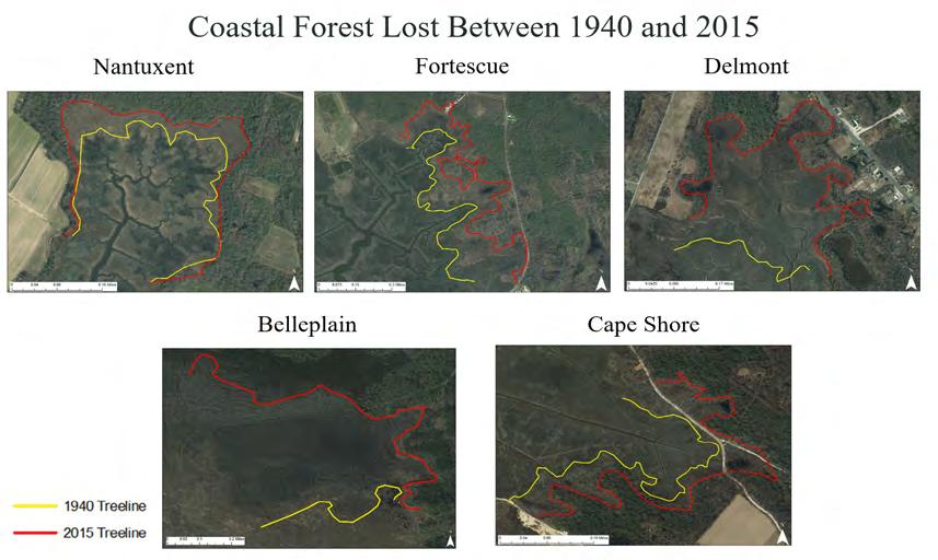
Coastal Forest Dieback in the Delaware Bay ..............................................
Rachael Sacatelli, Richard G. Lathrop, & Marjorie Kaplan
Rutgers, The State University of New Jersey
Julie
New
LeeAnn Haaf2
Partnership for the Delaware Estuary
Suggested citation
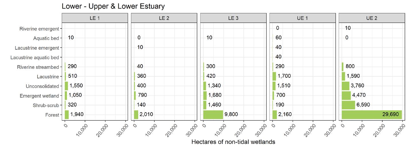
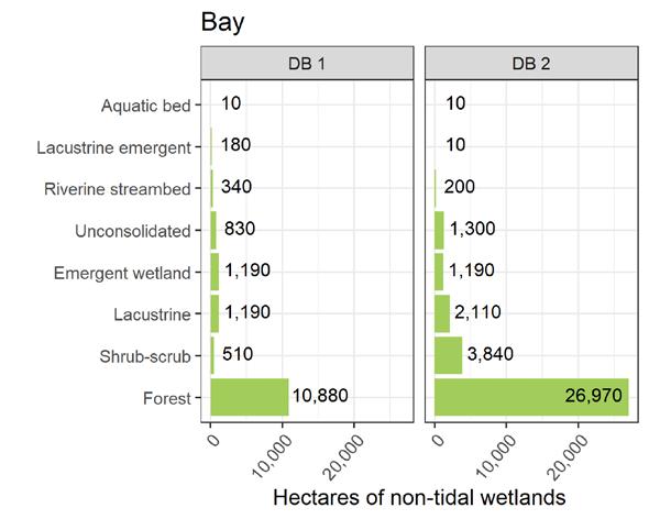
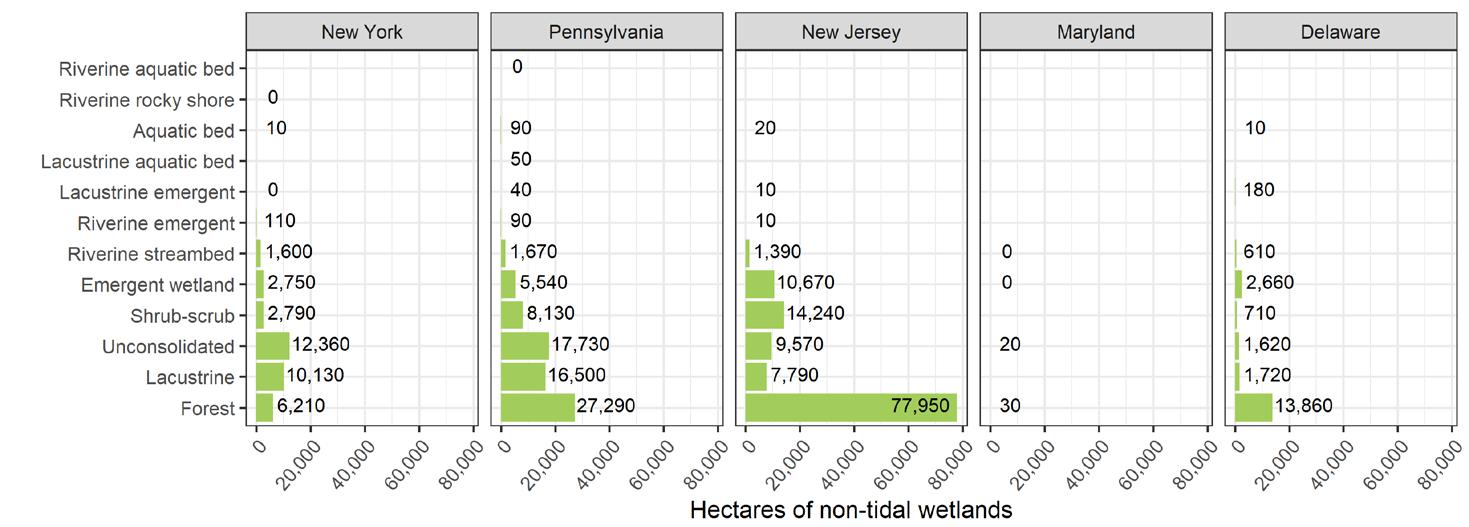
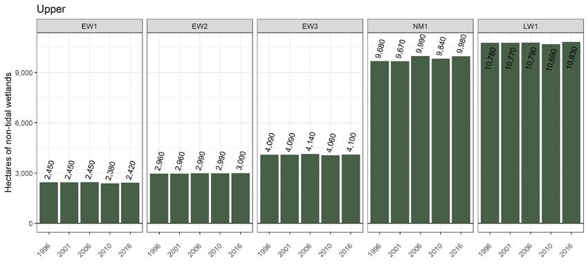
L. Haaf. 2022. Habitats: Non-tidal Wetland Acreage. Technical Report for the Delaware Estuary and Basin, L. Haaf, L. Morgan, and D. Kreeger (eds). Partnership for the Delaware Estuary. Report #22-05.
Mari-Beth DeLucia
The Nature Conservancy
Suggested citation
DeLucia, M. 2022. Habitats: Fish Passage. Technical Report for the Delaware Estuary and Basin, L. Haaf, L. Morgan, and D. Kreeger (eds). Partnership for the Delaware Estuary. Report #22-05. Richard Grabowski
6. Habitats
6.1 Forests
Abstract
Forests currently account for 49% of the land cover in the Delaware Estuary and Basin (1.6 million hectares). Forests in the Delaware Estuary and Basin are 80% deciduous, 14% mixed, and 6% evergreen. Over the period from 1996 to 2016, the total percentage of forest loss in the Estuary and Basin was over 24,000 hectares (1.5%). Future predictions indicate that forest conversion rates will continue as development continued and climate change adds extra pressure to forested ecosystems. Monitoring forested land cover is crucial to establishing restoration goals and developing actions to support good health of the Delaware Estuary and Basin.
Description of Indicator
Forests offer a myriad of ecosystem services including clean air and water protection, carbon sequestration, and climate change mitigation. Forest are critical habitats for an array of different plants and animals. Forests are also economically valuable to the timber and energy sectors. Access to forested spaces improves human quality of life through recreation, aesthetic value, a sense of place, in addition to providing other physical and mental health benefits. Sustaining these values for future generations requires collaboration among stakeholders, including state and federal agencies, landowners, industry professionals, conservation organizations, communities, and policymakers. Moreover, the collaboration between states is necessary when focusing on watershed-scale forest-related issues. In this chapter, we review the current status of forests using select metrics (from United States Forestry Service Forest Inventory and Analysis datasets; USFS FIA) and assess forest cover change using NOAA’s Coastal Change Analysis Program (C-CAP) data across the Delaware Estuary and Basin from 1996-2016. We used statespecific forestry action management plans to synthesize ongoing efforts, compare state priorities, and identify possible needs for the Estuary and Basin.
Data Sources
Forest cover data were obtained through NOAA’s C-CAP program through their online portal for the years 1996, 2001, 2006, 2011, and 2016 (for more information on the C-CAP dataset used here, see Chapter 1). The data from 2016 were used to determine the present status indicator for this section, with all years used to assess trends over time. C-CAP land cover data for forests were divided into broad forest type categories of evergreen forests, deciduous forests, and mixed forests (Table 6.1.1, Fig 6.1.1). For present forest conditions, modeled data layers from the USFS FIA were also used to show the distribution of more specific forest types, stand densities, stand size classes, as well as forest productivity. Additionally, for the present status, we review current state-level forested land ownership from state forestry action plans, as forest ownership has ramifications for how management actions are implemented. See Chapter 1 for a schematic representation of the Estuary and Basin assessment units and reporting hierarchy within the Delaware Estuary and Basin.
Table 6.1.1 Forest categories and type definitions
Category Definition Forest types
Deciduous
Evergreen
Mixed
Present Status
Forest Cover
Dominated by tree species that drop leaves in autumn; broadleaf and/or hardwoods
Dominated by tree species that retain leaves through winter; conifers/softwoods and nondeciduous hardwoods
Equally composed of deciduous and evergreen tree species
Oak / hickory
Maple / beech / birch
Elm / ash / cottonwood
Aspen / birch
White / red / jack pine
Spruce / fir
Longleaf / slash pine
Loblolly / shortleaf pine
Exotic softwoods
Oak / pine
Oak / gum / cypress
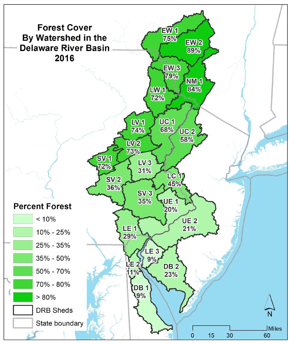
In 2016, there were 6,343 mi2 (1.6 million hectares) of forested land within the Delaware Estuary and Basin. Forested land makes up approximately 49% of all land cover within the Estuary and Basin. Forest cover is highest (>70%) in the Upper Region watersheds, but declines to 40-70% in the Central and Lower Region watersheds, with the Bay Region watersheds typically having <30% forest cover (Figure 6.1.2).
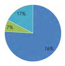
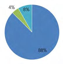
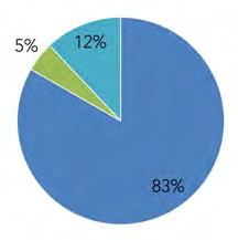
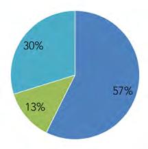
Forests across the entire Delaware Estuary and Basin are 80% deciduous, 14% mixed, and 6% evergreen. In the Upper, Lower, and Central Regions, deciduous forests account for >75% of forest cover with <10% evergreen forests, and the remainder being mixed forests. In the Bay Region, <60% of forests are deciduous, with 30% being mixed and 13% being evergreen. Generally, forest cover is low around the Philadelphia-Camden and Wilmington corridor of the Estuary (i.e., UE1, western UE2, and southeastern LE1; see Figure 6.1.2) due to the distribution of development and urbanization.
As the Estuary and Basin span a broad latitudinal gradient, with varying physiographic characteristics (e.g., geology, soil type, altitude), forest types vary among subregions (Figs 6.1.3-6.1.4). In the mountainous, northern watersheds of the Upper Region (i.e., Catskill mountains), forest types are dominated by maple/ beech/birch (Acer, Fagus, Betula spp) communities. Moving south towards the Pocono Mountains in the Central Region, forest communities shift to a dominance of oak/hickory (Quercus, Carya spp), a pattern which continues to the Lower and Bay Regions of the watershed. In UE2 and DB2 of the Bay Region, forest types also principally include loblolly/shortleaf (Pinus spp; a category that includes pitch pine)-these areas are associated with the New Jersey pine barrens.
Condition metrics
A suite of condition metrics are available from the USFS, but for this review, we consider productivity, stand density, diameter classes, stand ages, and ownership. Productivity indices identify potential tree growth modeled from the mean annual increment of fully stocked natural stands. Stand density indices reflect the modeled number of trees greater than 10” in diameter per acre, which can be used to surmise tree occupancy— it should be noted, however, that dense stands are not always in better ecological condition. Size and age classes reflect forest maturity, which could have an impact on forest biodiversity and resilience. Lastly, forest ownership is reviewed as a potential condition metric for forests because of the challenges associated with implementing large-scale management actions on privately-owned land.
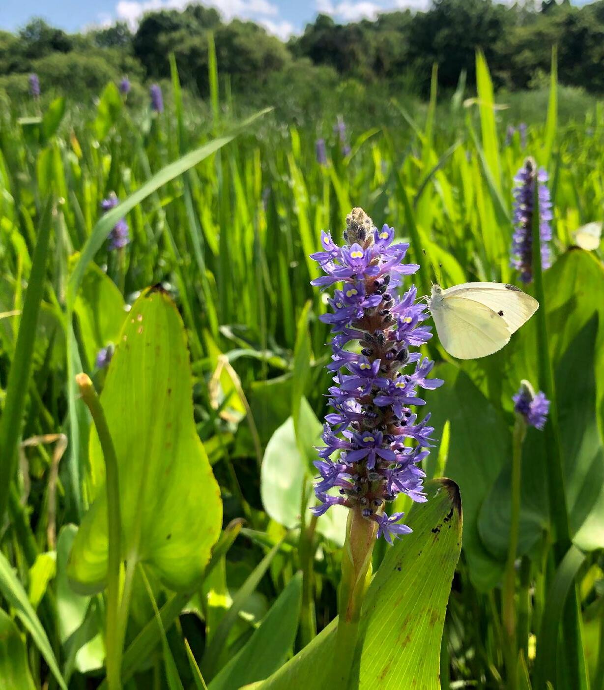
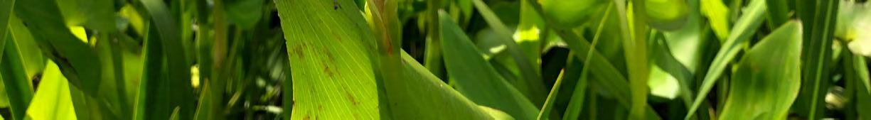
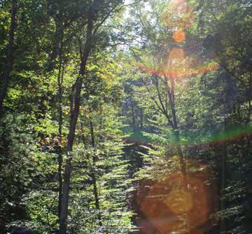
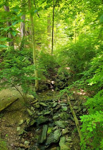
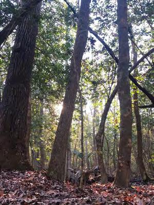
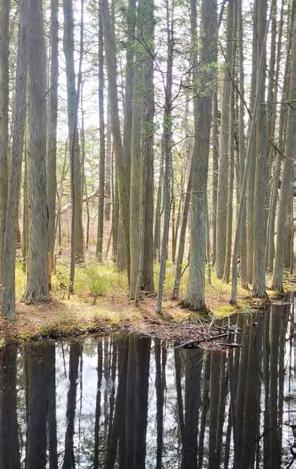
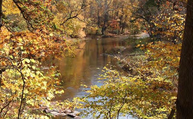
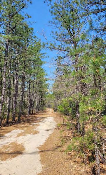
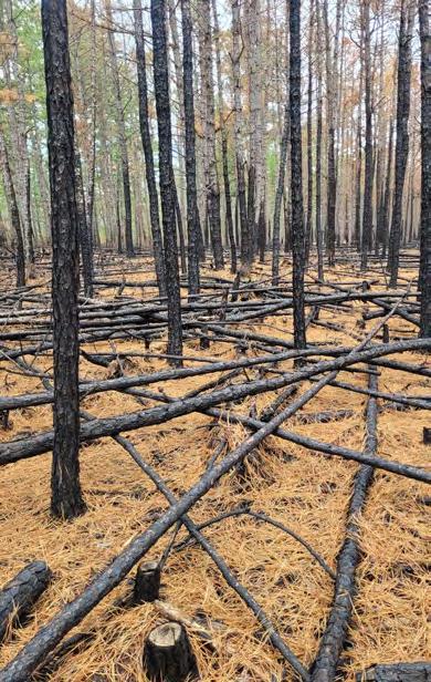
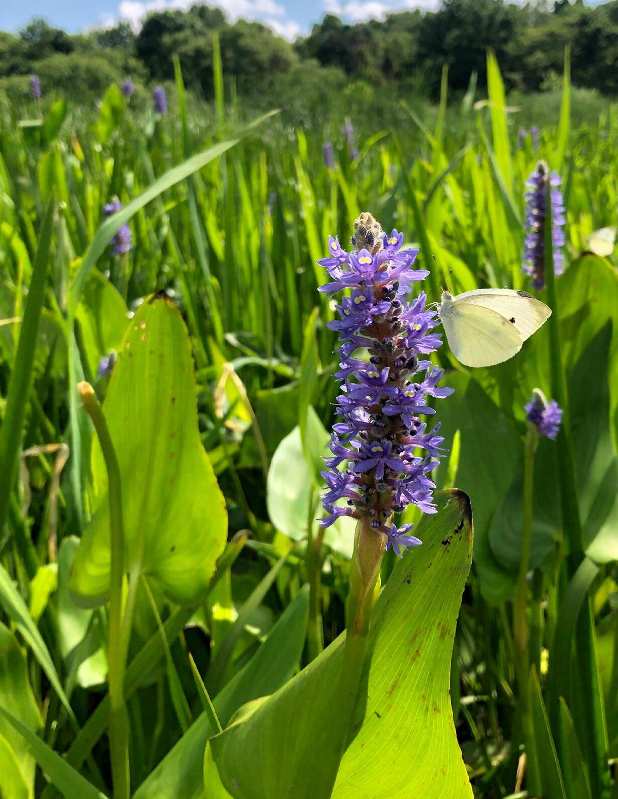
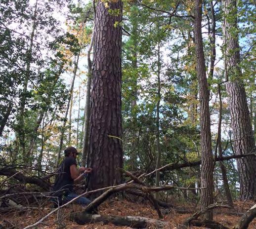
Figure 6.1.1 Diverse forests in the Delaware Estuary and Basin include hardwood forests (A, D, G), mixed forests (B), Atlantic white cedar swamps (E), and evergreen forests dominated by pines (C, with F showing forest structure after wildfire).
Photo by LeeAnn Haaf
Photo by Kelly Faller
Photo by Kelly Faller
Photo by Kelly Faller
Photo by Kelly Faller
Photo by Perkiomen Watershed Conservancy
Photo by Erica Rossetti
Figure 6.1.2 Forest cover in sub-watersheds of the Delaware Estuary and Basin (2016). Insets show the relative percentage of forest types in the (A) Upper (EW 1, EW 2, EW 3, NM1, LW 1), (B) Central (LV 1, LV 2, LV 3, UC 1, UC 2, LC 1), (C) Lower (SV 1, SV 2, SV 3, UE 1, UE 2, LE 1, LE 2, LE 3) and (D) Bay regions (DB 1, DB 2).
Forest Types
White / red / ja ck p ine
Sp ru ce / fir
Othe r ha rd woo ds
Oak / pi ne
Oak / hi ck ory
Oak / gu m / c y pres s
Ma pl e / b ee c h / bi rc h
Long le af / s la s h p ine
Lobl oll y / s ho rtl ea f pi ne
Ex oti c so ftwoo ds
El m / a s h / c otton wood
As
Sources: Esri, USGS, NOAA
Figure 6.1.3 Distribution of forest types across the Delaware Estuary and Basin from USFS FIA datasets (2018). Forest types are predominantly maple/beech/birch in the most northern watersheds, with a majority of the remaining watersheds of the Delaware Estuary and Basin dominated by oak/hickory. Forest types also include notable coverage by oak/gum/cypress along the Delaware River (southeastern UE 1, western UE2, eastern LE 2, and western LE 3). Further, central DB 1 and eastern UE 2 also have significant cover of loblolly/shortleaf pine.
Area (thousand acres)
Deciduous Evergreen Mixed
Figure 6.1.4 Forest cover by type in sub-watersheds of the Delaware Estuary and Basin (2016).
Indices for forest productivity and stand density match patterns associated with total forest cover across the Estuary and Basin (Figs 6.1.5-6.1.6). For instance, high productivity and stand densities are distributed in the Upper and Central regions where development and possible fragmentation is low. In the Philadelphia-Camden and Wilmington corridors, productivity and density indices are low, reflecting the intense urbanization there. In SV2, LV3, and northwestern parts of SV3, agriculture also dominates the landscape (see Chapter 1), and likely as a result, indices for forest productivity and density are low. In the areas of UE2 and DB2 that correspond with forests that benefit from protections of New Jersey Pinelands regulations, forest productivity and density indices are regionally high.
Across the states in the Estuary and Basin, forested lands are predominantly of large diameter classes (Fig 6.1.7). As forests grow older, they also grow larger. The majority of trees in the estuary region fall into a large diameter class, also considered “sawtimber”. The lack of diversity in size class across the region is directly related to the age structure of forests. Without the recruitment of saplings creating a heterogeneous forest structure, wildlife habitat and ecosystem services are reduced. New Jersey and Delaware, which have a less robust timber industry, are particularly vulnerable to this issue.
Across states, forests also lack diversity in age classes (Fig 6.1.8). Homogeneous forest age structures threaten the economic productivity and ecological health of forests. Forest age structure is related to time since past disturbance (Pan et al 2011). Overall, forests are maturing while regeneration rates have declined, resulting in a shortage of early successional forests as well as old-growth forests. Roughly 80 years ago, agriculture in the Northeast was largely abandoned and croplands were left to succeed into the mature forests we see today (Irland 1999, Thompson et al. 2013).
Forest ownership varied across the states within the Estuary and Basin. In New York and Pennsylvania, privately owned forests represent 74% and 70%, respectively, of each state’s forested land. In New Jersey and Delaware, privately-owned forests accounted for 48% and 47% of forested lands in each state. Stateinitiated management plans can face challenges when attempting to implement action items in privatelyowned forested systems. For instance, states with higher private ownership of forests face greater risks
Figure 6.1.5 Mean forest stand size from USFS FIA datasets (2018). Forest stands are predominantly large diameter (blue) across the Delaware Estuary and Basin.
Figure 6.1.6 Modeled mean forest productivity from USFS FIA datasets (2018).
NJ NY DE
Figure 6.1.7 State-wide forest stand-age class distributions for the four major states that comprise parts of the Delaware Estuary and Basin (2019).
(thousand acres) Area of forest land by stand-size class in Delaware Estuary, 2019
Figure 6.1.8 State-wide forest stand-size class distributions for the four major states that comprise parts of the Delaware Estuary and Basin (2019).
for lack of forest regeneration due to the high-cost burden of implementing action. In Pennsylvania, where a majority of forests are privately owned, few landowners have the resources to implement actions to support regeneration.
Trends
Current forest cover in the Delaware Estuary and Basin is likely only a fraction of what it was when only indigenous tribes managed the land. During European colonization, forest land was converted to agricultural land, a process that continued for centuries with clearing practices accelerating during the industrial age (Irland 1999, Thompson et al. 2013). As industrial technologies changed and development patterns changed in the early to mid-nineteenth century, forest clearing declined and reforestation likely increased while agricultural land in the eastern U.S. was abandoned (Irland 1999, Thompson et al. 2013). Since then, forest losses have likely remained small yet consistent over time as urban and suburban landscapes expand. Lastly, changing land-use history or anthropogenic manipulations have also contributed to landscape-wide forest community changes, such as the loss of American chestnuts through an introduced fungal pathogen and the proliferation of early-mid successional, mesic species such as red maple (Acer rubrum)(Irland 1999, Thompson et al. 2013).
Forest loss is a significant component in overall land cover changes in the Delaware Estuary and Basin, totally 93.5 mi2 or 24,200 hectares from 1996 to 2016. Forest cover change is a crucial indicator of overall watershed health, as the more forested a watershed, the better condition it is in terms of habitat, water quality, and ecosystem service provision. Over the period from 1996 to 2016, the total percentage of forest loss was 1.5%. Between each year of the analysis, there were variable rates of loss, with the most significant loss coming in the most recent period (between 2010 and 2016), with the loss of 0.5% of total forest cover. The second most significant drop occurred between 2001 and 2006, at a 0.4% loss.
Figure 6.1.9 shows the forest loss in square miles between each time span (i.e., between each year of available data) of the analysis, and across the entire period (1996 to 2016). The data are distinguished between Upper Basin (non-tidal) watersheds, Estuary watersheds, and the Basin as a whole. Figure 6.1.10 presents the changes in forest cover by time span as a percentage. Changes in forest cover also varied by forest type. The C-CAP data provide details on the forest cover type, including deciduous, evergreen, and mixed forests. Figures 6.1.9 and 6.1.10 also show the change for each of these three forest types across each 5-year period between 1996 and 2016. While the trend in forest cover is consistently down, with minor exceptions, there is variability in the percentage losses in the three categories of forest. The greatest loss in evergreen forest (slightly more than 0.6%) occurred between 1996 and 2001, while the greatest loss in deciduous forest cover (nearly 0.6%) occurred between 2010 and 2016. Only the period between 2001 and 2006 saw an overall increase in forest cover, for both evergreen and mixed forest types. All four states’ Forest Action Plans additionally suggest that the composition of forest communities is changing. These species shifts raise concerns about the future forest compositions, notably, their ability to provide critical food resources to wildlife. Potential reductions in mast species such as beech and oak towards species such as red maple will undoubtedly change forest trophic interactions.
Future Predictions
Forest cover has continuously declined across the Delaware Estuary and Basin, likely due to anthropogenic pressure. Anthropogenic pressure is likely to remain consistent or increase over time (see Chapter 1), and so, development or parcelization will continue to further net losses of forests, as well as fragmentation and lower habitat connectivity. Additionally, climate change is likely to drive large-scale community changes in forest cover and type (Forest Feature 1).
Rate of Forest Loss in the Delaware Basin, 1996-2016
Deciduous Evergreen Mixed
Figure 6.1.9 Total forest losses by type in the Delaware Estuary and Basin between 1996 and 2016.
Rate of Forest Loss in the Delaware Basin, 1996-2016
% Forest Loss in Period
Deciduous Evergreen Mixed
Figure 6.1.10 Rate of forest losses by type in the Delaware Estuary and Basin from 1996 to 2016.
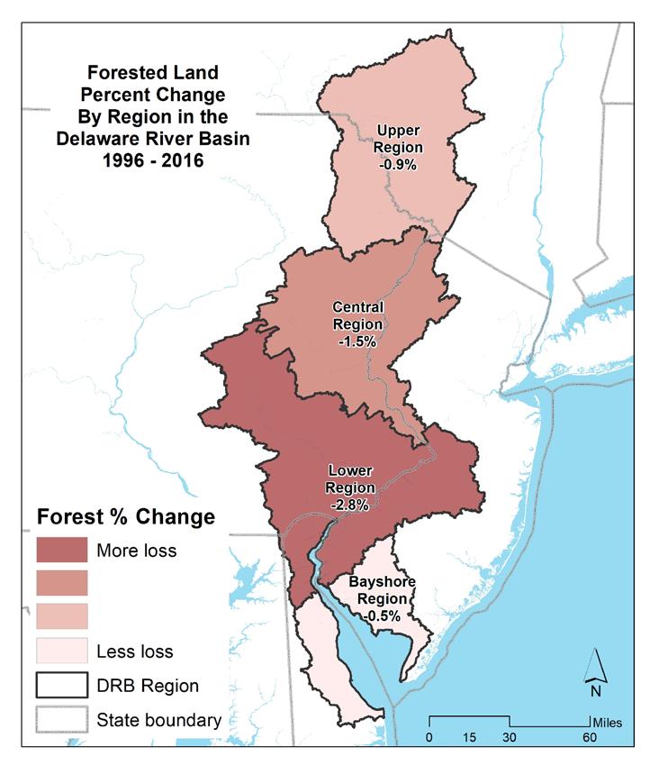
by Region
Figure 6.1.11 Forest cover percent change
of the Delaware Estuary and Basin (1996-2016).
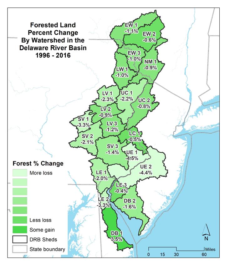
Figure 6.1.12 Forest cover percent change by watershed of the Delaware Estuary and Basin (1996-2016).
Damage-causing agents are likely to increase in influence across the Delaware Estuary as the climate changes, forests fragment, and populations increase. Invasive species are a focal point across all statespecific Forest Action Plans within the Estuary and Basin, with a heavy emphasis on rapid detection and monitoring as tools for management. The Estuary is especially susceptible to invasive pests as it is a hub for domestic and international transportation via roadways, railways, airways, and waterways. These pests are exacerbated by white-tailed deer population overabundance. Deer selectively browse native vegetation, giving invasive species a competitive advantage. Fire suppression aids the transport of native and non-native pests by creating dense, even-aged stands and can reduce species diversity, leaving the forest more susceptible to catastrophic damage.
Other notable drivers of future forest change include, but are not limited to, the inadequate regeneration of forests, biodiversity loss, forest maturation, and forested wetland acreage losses. All of these drivers reduce critical habitats for animal and plant species, especially those of conservation concern. Forest cover percent change by region and by watershed are depicted in Figures 6.1.11 and 6.1.12, respectively.
Actions & Needs
Every ten years, the federal Farm Bill requires states to compile a Forest Action Plan. These plans were first compiled in 2010. The recent 2020 Forest Action Plans represent the second iteration of this national forest planning effort which focuses on understanding the issues facing our nation’s forests and the actions necessary to mitigate those issues. Some important issues facing the states in the Delaware Estuary and Basin include:
• Forest conversion to development and agricultural land
• Fragmentation and parcelization into smaller forest tracts
• Regulations for private forest ownership make buying, holding, and maintaining forestland expensive, putting pressure on owners to sell or follow unsustainable practices
• Socioeconomic inequalities reflected in unequal rates of urban tree cover
• Forest fire suppression exacerbating wildland fire risk
As per the requirements of the Farm Bill, each state addressed the following three top national priorities in their action plans:
• Conserve and Manage Working Forest Landscapes for Multiple Values and Uses
• Protect Forests from Threats
• Enhance Public Benefit from Trees and Forests
Each state broke down the priorities into sub-issues and provided actionable forest protection measures. In Table 6.1.2 we present a summary of priority items proposed in state-specific forestry action plans for New York, New Jersey, Pennsylvania, and Delaware.
Summary
Forests provide important ecosystem services such as reducing stormwater runoff and cleaning our air and water. Across the watershed, forests account for roughly half of the total land cover, but this is likely only a fraction of what it was 400+ years ago. Although forest types vary by region, states in the Estuary have similar issues with connectivity, cover, and condition. Development around the estuary has been
Topic New Jersey
Priorities
• Tree density
• Forest age structure
• Species of Concern
• Biodiversity
• Fragmentation, invasive species, land use change/disturbance, and climate change
• Climate and Carbon
• Fragmentation and Habitat
• Damage-Causing Agents
• Keep New York’s forests as forests (“Forests as Forests”)
• Keep New York’s forests healthy (“Healthy Forests”)
• Ensure forests benefit humans and all living creatures (“Forests for People”)
• Support, protect, and appreciate New York’s forests (“People for Forests”)
• Defending forests from invasive plants and insects
• Excessive forest clearing and fragmentation
• Worsening forest regeneration
• Diversity, equity, and inclusion
• Indigenous knowledge/ values and commitment to an increased level of engagement
• Forest Health and Functionality
• Forest Markets
• Sustainable Forest Management
• Public Awareness and Appreciation of Forests
• Reducing threats of development, fragmentation/ parcelization
• Soil and water quality protection and enhancement
• Land Use Change
• Forest Health
• Sustainable Forest Management
• Climate Change
• Communicating Natural Resource Values
• Energy Management & Development
• Wildland Fire and Public Safety
• Plant and Animal Habitat
• Forest-related Economy and Jobs
• Forest Recreation
• Water and Soil
• Conserve and manage working forest landscapes for multiple values and uses.
• Protect forests from threats.
• Enhance public benefits from trees and forests.
Possible risks
White-tailed deer over abundance, disease, fragmentation/parcelization/development, climate change, invasive species
increasing and will continue to increase. Forest losses have slowed since mid-century, but losses have continued overall, with slightly higher recent losses (0.5% per year from 2010-2016). Adaptively managing remaining forests, and preserving forests where possible, will be critical to their future functioning and the health of the Estuary and Basin.
Forests are facing several issues, such as but not limited to, age/size class distribution, reduced regeneration rates, conversion, and damage-causing agents. The state-specific forestry action plans provide a framework for understanding key issues to forests in each state, possible action items, and gaps in management practices. This review identifies similarities, strengths, and possible gaps for management across the watershed. Reductions in fragmentation, more forest protected lands and/ or state management areas (purchases, easements, etc), increased prescribed burning (reduced fire suppression), ecological-based management tactic implementation (increase age class diversity and biodiversity, etc), and support for urban forestry are key themes to address moving forward.
References
Delaware Department of Agriculture Forest Service, 2020, Delaware Forest Resource Assessment, https://delawaretrees.com/2020_del_forest_resource_assessment.pdf.
Forest buffers. Chesapeake Bay Program. (n.d.). Retrieved June 24, 2022, from https://www. chesapeakebay.net/issues/forest_buffers
Irland LC. 1999. The Northeast’s changing forests. Cambridge, MA: Harvard University Press.
New York State Department of Environmental Conservation, 2020, New York State Forest Action Plan, https://www.dec.ny.gov/docs/lands_forests_pdf/nysfap.pdf.
National Oceanic and Atmospheric Administration, Office for Coastal Management. “C-CAP Regional Land Cover.” Coastal Change Analysis Program (C-CAP) Regional Land Cover. Charleston, SC: NOAA Office for Coastal Management. Accessed June 2022 at www.coast.noaa.gov/htdata/ raster1/landcover/bulkdownload/30m_lc/.
Pan, Y., Chen, J.M., Birdsey, R., McCullough, K., He, L. and Deng, F., 2011. Age structure and disturbance legacy of North American forests. Biogeosciences, 8(3), pp.715-732. https://journals. plos.org/plosone/article?id=10.1371/journal.pone.0072540
Pennsylvania Department of Conservation and Natural Resources Bureau of Forestry, 2020, Pennsylvania Forest Action Plan, http://elibrary.dcnr.pa.gov/ GetDocument?docId=3861659&DocName=PA%20Forest%20Action%20Plan%202020.pdf.
State of New Jersey Department of Environmental Protection NJ Forest Service, 2020, New Jersey State Forest Action Plan, https://nj.gov/dep/parksandforests/forest/njsfap/docs/njsfapfinal-12312020.pdf.
Thompson, J.R., Carpenter, D.N., Cogbill, C.V. and Foster, D.R., 2013. Four centuries of change in northeastern United States forests. PloS one, 8(9), p.e72540.
Forest Feature 1
Loblolly Pine and Eastern Hemlock Distributional Shifts with Climate Change
Kelly Faller & LeeAnn Haaf Partnership for the Delaware Estuary
Climate change will have sweeping effects on forest health and composition in the future. One of the many impacts of human-induced climate change is increasing temperature. Temperatures in the Mid-Atlantic are projected to increase 0.5 to 4.2°C (2.2 to 7.6°F) by the end of the century. With these changes, we expect that the current distribution of tree species will shift northward in response to warming temperatures. The Delaware Estuary, sitting at the confluence of many tree species’ northern or southern range extent, will likely see forest community compositional shifts as species distributions expand poleward to match their temperature thresholds.
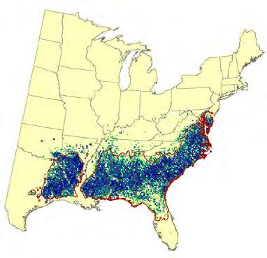
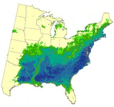
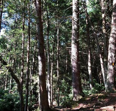
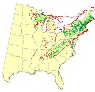
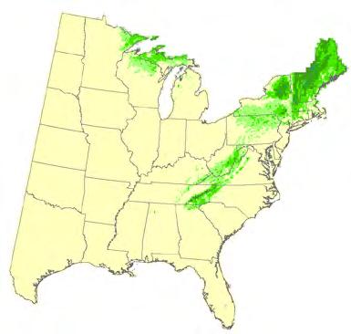
This feature focuses on the climate change-induced species distribution changes of loblolly pine (Pinus taeda; Fig 6.1.13A) and eastern hemlock (Tsuga canadensis; Fig 6.1.13B). These species are valuable examples of range shifts as the Delaware Estuary and Basin is the southern-most extent, and/or elevation limit, of eastern hemlock (Fig 6.1.13C) and the northern-most extent of loblolly pine (Fig 6.1.13D). Hemlock and loblolly pine are both commercially valuable woods and their shifting ranges will impact the timber industries throughout the states that constitute the Delaware Estuary and Basin.
Here we present USFS Climate Change Atlas (v 4.0) models of loblolly pines and eastern hemlock distributional changes based on current distributional, physiographic, and climatic information (ButlerLeopold et al. 2018). We chose to showcase predicted distributional changes of loblolly pine and eastern hemlock under the highest emission climate scenario predicted by the Intergovernmental Panel on Climate Change (RCP 8.5). This climate prediction is frequently referred to as “business as usual”, as it predicts climate change if there was no change in policy or action with respect to carbon dioxide emissions.
Under continued carbon dioxide emissions, loblolly pine will likely become more common in the lower estuary as its distribution shifts northward, further into New Jersey and Pennsylvania (Fig 6.1.13E). Contemporaneously, as temperatures warm, eastern hemlock is likely to experience northward shifts outside of the watershed— until this species becomes rare within the Basin (Fig 6.1.13F).
Citations
Butler-Leopold, P.R., Iverson, L.R., Thompson, F.R., Brandt, L.A., Handler, S.D., Janowiak, M.K., Shannon, P.D., Swanston, C.W., Bearer, S., Bryan, A.M. and Clark, K.L., 2018. Mid-Atlantic forest ecosystem vulnerability assessment and synthesis: a report from the Mid-Atlantic Climate Change Response Framework project. Gen. Tech. Rep. NRS-181. Newtown Square, PA: US Department of Agriculture, Forest Service, Northern Research Station. 294 p., 181, pp.1-294.
USFS Climate Change Atlas, Trees, v 4.0. 2022. <https://www.fs.fed.us/nrs/atlas/tree/> Accessed July 5, 2022.
Intergovernmental Panel on Climate Change (IPCC). 2022. Climate Change 2022: Impacts, Adaptation and Vulnerability. <https://www.ipcc.ch/report/ar6/wg2/> Accessed July 5, 2022.
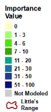
Figure 6.1.13 Distributions of loblolly pine ( Pinus taeda, A) and Eastern hemlock ( Tsuga canadensis , B) in the eastern United States from current (C, D, respectively) to future distribution under RCP 8.5 (E, F) modelled by USFS FIA.
Technical Report for the Delaware Estuary and Basin Partnership for the Delaware Estuary— Host of the Delaware Estuary Program
6.2 Submerged Aquatic Vegetation
Description of Trial Indicator
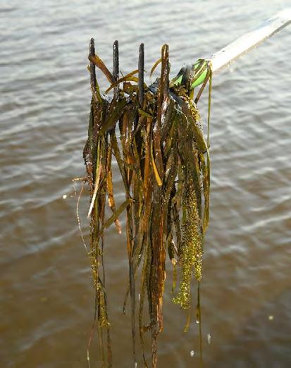
Submerged aquatic vegetation (SAV) is an essential habitat for fish and other wildlife (Fig 6.2.1). It provides spawning, nursery, and protective habitat to juvenile fish and bivalves such as freshwater mussels (Lubbers et al. 1990; Heck et al. 2003). SAV services include shoreline stabilization, carbon sequestration, nutrient filtration, sediment entrapment and wave energy dissipation (Kemp et al., 1984; Orth et al., 2010; Ward et al., 1984; Waycott et al., 2009; Jaskinski et al., 2021). Despite these ecologically important attributes, historical SAV studies in the tidal Delaware Estuary are limited (Schuyler, 1988; Schuyler et al., 1993).
For this report, submerged aquatic vegetation is being piloted as a trial indicator. To create a foundation for protecting and ultimately restoring SAV habitat in the tidal Delaware Estuary, a baseline understanding of the distribution, density, and composition of SAV was needed. Since 2017, acoustic data has been collected and analyzed to begin to characterize these metrics. Furthermore, preliminary observational data has been recorded to start to understand habitat suitability, interannual trends and factors impacting long-term stability. Currently, there is not enough data over time to analyze trends and methods are still evolving. Therefore, a full indicator report is not currently feasible. This trial indicator reports some preliminary data and observations but is not able to discuss potential indicators of watershed health.
Methods
Typically, quantifying SAV is assessed through annual aerial images that are used to map SAV beds. Aerial flights and assessment of imagery are dependent on favorable water clarity. The Delaware Estuary is a naturally turbid watershed making aerial imagery an unreliable method for quantifying SAV extent. Because of this, hydroacoustic surveys were determined to be the most suitable and effective method for detecting and mapping SAV.
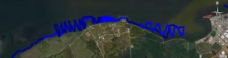
Using an echosounder mounted to a vessel, transects parallel to the shoreline were surveyed. The distance off the edge of the shoreline varies depending on the bathymetry and bottom type. Parallel transects were used to identify ‘presence/absence’ of SAV. When SAV was confirmed along the
Figure 6.2.1 SAV captured on a telescoping rake in the Tidal Delaware River.
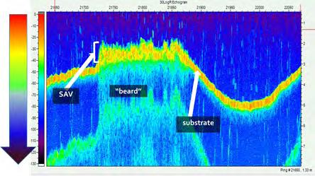
parallel transect, transects perpendicular to shore were surveyed to determine the spatial extent of the beds. The pattern to delineate the bed is similar to ‘mowing the lawn’ where the boat moves in lines perpendicular to shore to map the entire length and width of the bed. Figure 6.2.4 shows this collection pattern. Using Visual Acquisition, Biosonics Field Data Collection Software program, while pinging the echosounder, an echogram would display the bottom substrate and where SAV might be present. During perpendicular transects, field verification was used by dropping a telescoping rake at random points throughout the bed. Where possible, species identification was noted. Species composition has not been a regular variable measured in the annual acoustic survey, however where possible coordinate pins were dropped on the software and field notes captured species. Species that were identified include Vallisneria americana. In future years, there is plans to have a more concerted effort to inventory species identification.
Ground-Truthing
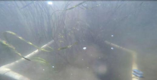
EPA’s Scientific Dive Unit completed numerous dives to field verify the echosounder data as well as to collect other scientific field data. Divers used quadrats to determine percent coverage as well as species composition and noted the presence of bivalves, if observed. Divers had difficulty collecting data due to low visibility, strong currents, and the heavy accumulation of fine sediments within the SAV beds (Fig 6.2.5). Select long-term monitoring stations were piloted with the intent of having annual scientific dives.
Post-Processing
After the data is collected, it is post processed using BioSonics Visual Aquatics (formerly Visual Habitat). The software interpolates the data in two phases. First, the program auto detects and delineates the bottom surface drawing the hard bottom providing the bathymetry for the area. In areas of high density SAV beds, some manual editing is required using the ‘draw tool’ to identify and delineate the bottom substrate. After the bottom is defined, the program then auto-detects and delineates the vegetation canopy. Some editing may be required to further delineate the canopy using the software’s pen tool. Processed data were exported to comma separated value (CSV) format to facilitate loading into a geographic information system (GIS) platform and a database management system.
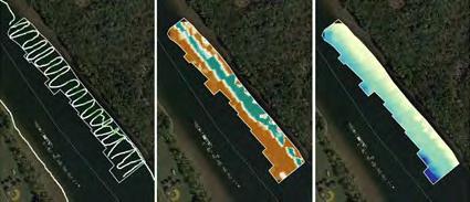
Inverse distance weighting (IDW) technique was then used to interpolate the data (Fig 6.2.6). IDW is a nearest neighbor approach that relies less on geo statistics and underlying assumptions. IDW assumes that points with close proximity geographically will tend to have similar values. This high-density survey
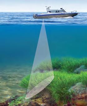
Figure 6.2.2 Example of a single beam echosounder sending pings down the water column (image from BioSonics).
Figure 6.2.3 Example of a single beam echosounder.
Figure 6.2.4 Example of boat tracks for collection. The tight zigzag patterns mimics ‘mowing the lawn’.
allowed the interpolation of raster datasets depicting plant coverage. The interpolated raster data was then clipped 1 meter from the closest sample point to ensure only areas covered by the survey were represented. Coverage is reported in the percent of pings that recorded vegetative cover (i.e., 0, 20, 40, 60, 80, 100).
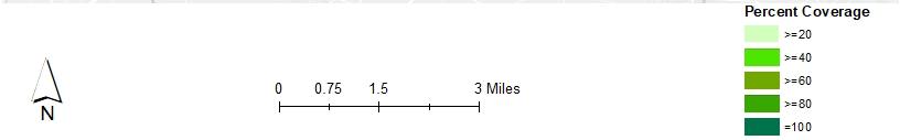
Data from 2017-2020 are available online for viewing and download online. In 2017 and 2018, data was collected parallel to shore to determine the presence or absence of SAV. In 2019, the survey refined its methods and limited scope allowing more detailed bed delineation. The 2020 and 2021 field season was more limited due to travel restrictions from COVID-19.
Present Status
The project, which focused on inventorying the distribution and density of SAV, has completed five years of monitoring (2017-2021). The first two years, 2017-2018, set out to completely map the Delaware Estuary which includes the tidal Delaware River and the Delaware Bay. However, no SAV was identified in the meso- or polyhaline zones of the river from approximately the Delaware Memorial Bridge south to the mouth of the Delaware Bay. Therefore, starting in 2019, the survey scope was re-focused to the tidal Delaware River which includes the head of tide near Trenton, NJ down to the maximum turbidity zone near the Delaware Memorial Bridge.
There are a few possibilities why no SAV (seagrasses) were found in meso- and polyhaline areas. One is that species like Zostera marina never thrived in the system historically (Schuyler 1988; Schuyler et al., 1993). Another possibility is that the survey did not look in the right areas and/or at the right time. Since time and resources were a factor, the decision was made to focus on the freshwater tidal where SAV was found and thriving.
Figure 6.2.6 A time series showing the process of interperolation using IDW.
Figure 6.2.5 A quadrat used by scientific divers quantifying the percent coverage of SAV.
Step 1
Step 2
Step 3
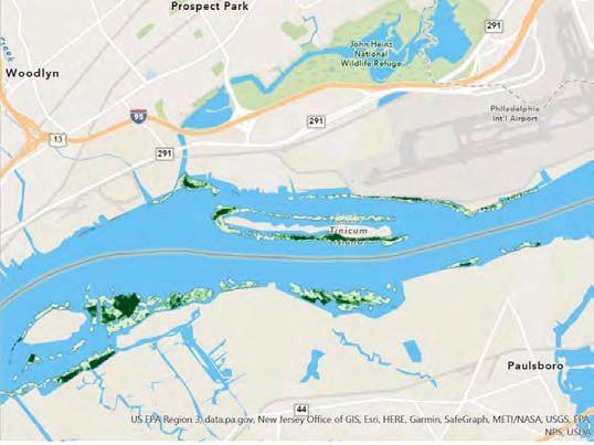
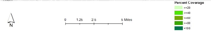
Basic analysis of distribution and density of SAV was analyzed for 2019 and was summarized among the Delaware River water quality zones (Table 6.2.1). Coverage is reported in the percent of pings that recorded vegetative cover (i.e., 0, 20, 40, 60, 80, 100). The map of Little Tinicum Island (Fig 6.2.7) and the surrounding areas demonstrate the percent coverage of SAV. The darker the shade of green, the denser the bed is. As the survey continues, time-series trends of changes in bed density and size will be able to be collected and shared to determine the stability of SAV health in the system.
Table 6.2.1 Summary of SAV distribution and density in Delaware River water quality zones.
Water Quality Zones
SAV Density (Acres)
Zone 2 1213
Zone 3 628
Zone 4 1352
Zone 5 109
Figure 6.2.7 A map of Little Tinicum Island in the Delaware River displaying the density of SAV. Dark green indicates high plant density.
Zone 1 – No surveys completed as this area is not tidal.
Zone
2
– Head of tide to Pennypack Creek
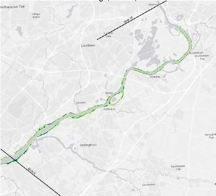
The head of tide starts in Zone 2 near Trenton, NJ. SAV beds from Roebling, NJ north to the survey limit are narrow and close to the banks (Fig 6.2.8). Bathymetry within this area consisted of a narrow shallow shelf close to the banks which is likely a limiting factor for SAV. Overhanging terrestrial vegetation also shades portions of the banks. South of Roebling to the Burlington Bristol Bridge, SAV beds get broader as the bathymetry of the river provides greater shelf areas and favorable depths that allow for light penetration at mean high water and remain submerged at mean low water. Areas south of the Burlington Bristol Bridge to Pennypack Creek have broader beds and greater shelf area with favorable water depths. Some beds, although not continuous, extend almost 150 m (500 ft) from the shoreline toward the center of the river, with multiple bands of beds.
Zone 2 also contains Newbold and Burlington Islands. The Newbold Island back channel was not surveyed due to water depths being too shallow for boat passage. SAV beds were identified along the main channel side of the island, along a stone revetment on the southern portion of the island, as well as the northern forested portion of the island. The southern tip of Burlington Island has a significant bed, which was thoroughly surveyed in 2019-2021. The channel side of the island, as well as portions of the back channel of the island, had SAV beds in 2019. The areas lacking SAV beds were deeply scoured, dredged for marina space, and/or too exposed at low tide.
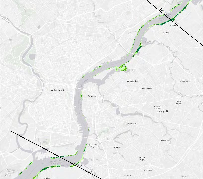
Zone 3 – Pennypack Creek to Big Timber Creek
SAV in Zone 3 was most abundant north of Petty Island (Fig 6.2.9). A broad bed thrives just south of the Pennsauken Creek. A bed on the northern tip of Petty Island was also intensely surveyed in 2019-2021. The cove associated with the northern tip of Petty Island has significant bed(s) consisting of a variety of different species. However, the channel ward side of the island as well as most of the back channel of the island SAV has not been observed. In 2021, a small area was observed just south of the bridge to access the island. From Petty Island to the south of the Walt Whitman Bridge, SAV is limited to areas that have not been dredged. The survey did not investigate within the old piers or behind structures due to navigation hazards, but SAV may be present within these areas. Downstream of the Philadelphia/Camden port facilities and along the bulkhead of the Navy Yard, the beds get broader as the bathymetry of the river provides greater shelf area and at favorable depths for SAV. The beds are close to the riverbanks. The Navy Yard site is another location where thorough data has been collected.
Figure 6.2.8 SAV coverage, Zone 2, 2019.
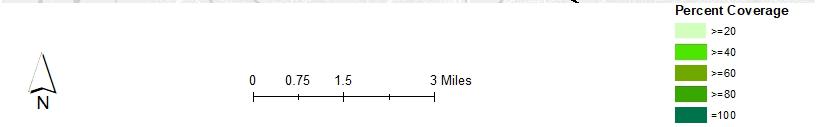
Zone 4 - Big Timber Creek to Marcus Hook/Raccoon Creek
Zone 4 contains abundant SAV beds (Fig 6.2.10). Many of the areas lacking SAV along the main channel, however, have been dredged. The Red Bank Battlefield area has significant bed(s) consisting of a variety of different species. A submerged wave screen located north of Chester Island supports a large bed of SAV that sits over 600 m (2,000 ft) channel ward of the shoreline. Another large bed is established at the mouth of Darby Creek. From Darby Creek south along the Pennsylvania shoreline, SAV is sparse, and the area has been dredged.
This Zone contains Tinicum and Chester Islands. The channel ward side of Tinicum Island consists of narrow beds of SAV close to the shoreline. The southern tip of the island contains a broad bed that stretches into the back channel. At the back side of the island, SAV is sparse but emergent spatterdock (Nuphar advena) is prevalent. The portion of back-channel along Hog Island Road also supports a broad bed of SAV that narrows and transitions to spatterdock as the road turns north. Chester Island has a large SAV bed on the south side of the submerged wave screen discussed above. There is also a bed along
Figure 6.2.9 SAV coverage, Zone 3, 2019.
a revetment on the back channel of the island and a small dense bed on the southern tip of the island. Moving south, the amount of SAV decreases significantly.
Zone 5 - Marcus Hook – Raccoon Creek Delaware State line south
SAV in Zone 5 is minimal and sparse (Fig 6.2.11). While the bathymetry and water depths would support SAV, very little SAV was observed in the 2019 survey. The SAV that was observed was mostly on the New Jersey side, close to the Commodore Barry Bridge. A small amount of SAV was observed along the New Jersey coastline. This area is the maximum turbidity zone in the Estuary and high concentrations of suspended sediments may interfere with light reaching the bottom substrate. Additional studies are required to determine the limiting factors of SAV distribution in this Zone.
Technical Report for the Delaware Estuary and Basin Partnership for the Delaware Estuary— Host of the Delaware Estuary Program December 2022 | Report No. 22-05
Figure 6.2.10 SAV coverage, Zone 4, 2019.
2019.
Regulatory Authorization
Impacts on SAV must be considered during the decision-making process to issue a permit for dredge and/or fill material. Data from this study is being used by applicants and agencies to review proposed project sites for potential impacts on SAV beds. If SAV is present within the project area, the applicant may need to consider alternative locations to avoid and minimize the negative impacts on SAV. If SAV cannot be avoided and a permit is issued, mitigation may be required.
Past Trends
There is a lack of information on the historic distribution of SAV species in the Delaware Estuary (Schuyler, 1988; Schuyler & Kolega, 1993). It was once believed in the scientific community that SAV did not thrive in this system due to the limited light availability, turbidity, excess nutrients, and/or dredging activity occurring in the system. Some of these limiting factors, like turbidity, are natural features of the Delaware Estuary. Up until 2011-2012, however, researchers lacked adequate equipment and technical expertise to properly inventory the size, extent, and species of the beds. Also, the Philadelphia Water Department (PWD) performed a study in 2011 in which they observed emergent and submerged species, but the area of study did not extend beyond the city limits.
In 1988, the Academy of Natural Sciences published the most cumulative historical and present account of SAV plant diversity in the tidal Delaware River and its tributaries. The report indicated that no previous
Figure 6.2.11 SAV coverage, Zone 5,
work had been done on submergent or planmergent (plants with floating leaves) in the watershed. It was reported that numerous plants of Vallisneria americana, Myriophyllum spicatum, Elodea nuttallii, and Najas flexilis were present in the portion of the Estuary between Trenton and Philadelphia. That is consistent with the preliminary plant identification found in the current research. In this report, it was acknowledged that the larger tidal range might play a factor in plant diversity in the main Delaware River channel. It was concluded that some plants that appeared prior to the 1930s were then found to be absent in the river. Other plants remained or retreated to tributaries where tide ranges were smaller or did not span as far down the river as once before. This study showed that SAV diversity declined. Although this study looked at species distribution, it did not synthesize plant coverage or bed densities throughout the watershed. This study provided valuable information on species occurrences but did not indicate historical SAV bed density or areal cover, making it difficult to measure what the historical acreage of SAV in the tidal Delaware River was (Schuyler, 1988; Schyler et al. 1993).
Understanding the role of SAV in the Delaware Estuary and its impact on water quality and habitats has been identified as an important data gap. A 2006 white paper on the Status and Needs of Science in the Delaware Estuary authored by members of the Delaware Estuary Scientific and Technical Advisory Committee identified Submerged Aquatic Vegetation as data gap particularly given their importance to benthic communities (Kreeger et al. 2006). The 2021 Delaware Estuary Monitoring Inventory and Needs Assessment also identified SAV as a top monitoring priority (Partnership for the Delaware Estuary, 2021).
Future Predictions
SAV habitat in the tidal Delaware River is subject to many potential threats. However, without long-term data, it is difficult to predict how these changes could impact SAV survival. SAV in the tidal Delaware River has been subjected to historical dredging and fill events over time and has survived, despite the altered location of the riverbanks, changing bathymetry, and increase in sedimentation. Continuing to monitor the effects and understanding the impacts of physical changes is important to SAV protection.
Climate change is another threat to SAV health. As sea levels rise, increasing water heights with few shallow areas left to retreat due to hardened shorelines could cause significant losses to SAV in the Delaware. Shifting salt lines, another result of sea level rise, has the potential to impact freshwater SAV habitat. As storms increase in the watershed, large flushing events may lead to significant increases in nutrient and sediment loads that impact SAV growth by limiting light. Water quality improvements in the Delaware River could lead to significant SAV expansion. Improved water quality might also provide improved ways to monitor (i.e., aerial imagery or drones) and allow researchers to access tributaries and other shallower bodies within the estuary.
Actions and Needs
Several actions are needed to understand the value that SAV may play in the Delaware Estuary.
Species
Inventorying and their distribution
This project has largely been focused on capturing the broad distribution and density of SAV beds in the Tidal Delaware River. Researchers capture sample grabs at select sites throughout the survey and note species collected, but no systematic approach to fully capturing in-depth underwater analysis of species diversity and geographic distribution of those species have been undertaken. Understanding the species diversity and their distribution could aid in future restoration projects and capture SAV ecosystem services.
Understanding Habitat Suitability
SAV has specific habitat and growth requirements, usually determined by light attenuation. The tidal Delaware River has an approximate 1.8 meter (~6 feet) tidal range that is also subjected to activities like dredging. Understanding the factors that determine SAV suitability is necessary to understand potential restoration and preservation. It’s important to also understand what species can thrive under varying conditions such as large tidal ranges, changes in water quality variables, exposure to high energy, increases in sedimentation, and loss of light. Additionally, it is critical to understand the necessary sediment type and shoreline needed to create and maintain SAV habitats. To best preserve and restore SAV habitat, studies are needed to understand the physical, chemical, and biological factors required for SAV beds to thrive.
Piloting Restoration and Planting
SAV restoration is an important consideration for the Delaware River watershed. SAV provides many ecosystem services and increasing SAV distribution would improve water quality and provide essential habitat to key species. Little information is available to guide restoration managers on how best to restore SAV beds. Developing restoration guides that specify when to collect seeds, plugs or transplant and where and when to plant them is needed for successful restoration.
Summary
SAV is a vital habitat that provides many ecosystem services and protecting and restoring it is essential to supporting clean and healthy watersheds. SAV in the tidal Delaware Estuary is expansive and diverse, contrary to the previously accepted notion that this naturally turbid system could not support abundant SAV. Continuing to monitor SAV and establishing it as an indicator of water quality and benthic habitat is an important next step to understanding the overall health of the Delaware Estuary.
References
Heck, K. L., Hays, G. C., & Orth, R. J. (2003). Critical evaluation of the nursery role hypothesis for seagrass meadowns. Marine Ecology Progress Series 253, 123-136.
Jaskinski, D., Gurbisz, C., & Landry, B. (2021). Small-scale SAV Restoration in Chesapeake Bay: A Guide to the Restoration of Submerged Aquatic Vegetation in Chesapeake Bay and its Tidal Tributaries. cheapeakebay.net.
Kemp, W. M., Boynton, W. R., Twilley, R. R., Stevenson, J. C., & Ward, L. G. (1984). Influences of submersed Vascular Plants on Ecological Processes in Upper Chesapeake Bay. In The Estuary as a Filter (pp. 367-369). Academic Press.
Kreeger, D., Tudor, R., Sharp, J., Kilham, S., Soeder, D., Mawell-Doyle, M., Kraeuter, J., Frizzera, D., Hameedi, J., and Collier, C. (2006). White Paper on the status and needs of science in the Delaware Estuary. Wilmington: Partnership for the Delaware Estuary.
Lubbers, L., Boynton, W. R., & Kemp, W. M. (1990). Variations in structure of estuarine fish communities in relation to abundance of submersed vascular plants. Marine Ecology Progress Series 64, 1-14.
Orth, R. J., Williams, M. R., & Marion, S. R. (2010). Long Term Trends in Submersed Aquatic Vegetation in the Chesapeake Bay, USA, Related to Water Quality. Estuaries and Coast, 33, 1144-1163.
Partnership for the Delaware Estuary. (2021). Monitoring Inventory and Needs Assessment for the Delaware Estuary: Addendum to the 2019 Comprehensive Conservation and Management Plan
for the Delaware Estuary. Wilmington, DE.
Schuyler, A. E. (1988). Submergent and Planmergent Flora of the Freshwater Portion of The Delaware Estuary. In Ecology and Restoration of the Delaware River Basin (pp. 157-168). Philadelphia: Pennsylvania Academy of Natural Sciences.
Schyler, A. E., Anderson, S. B., & Kolaga, V. J. (1993). Plant zonation changes in the tidal portion of the Delaware River. Academy of Natural Sciences of Philadelphia, (pp. 263-266). Philadelphia.
Ward, L. G., Kemp, W. M., & Boynton, W. R. (1984). The influence of waves and seagrass communities on suspended particulates in an estuarine embayment. Marine Geology, 59(1-4), 85-103.
Waycott, M., Duarte, C. M., Carruthers, T. J., Orth, R. J., Dennison, W. C., Olyarnik, S., . . . Williams, S. L. (2009, July 28). Accelerating loss of seagrasses across the globe threatens coastal ecosystems. The Proceedings of the National Academy of Sciences, 106(30).
6.3 Wetlands
Wetlands are areas where water inundates soils, or saturates at or near the surface of the soil all year, seasonally, or periodically. The gradient of saturated conditions in wetlands create characteristic hydric soils, which in turn supports specially adapted plants (hydrophytes). Wetlands also have key ecosystem functions, or services, that support clean water and provide habitat for a variety of plants and animals. The status and trends in wetland cover are therefore important indicators of the health of the Delaware Estuary and Basin.
In Chapter 1, land cover classes were assessed broadly, with both forests and wetlands constituting “natural land cover.” Here, in Chapter 6.3, we specifically summarize wetland cover patterns. In the following sections of this chapter, we further address the two main classes of wetlands in the Estuary and Basin: 1) tidal wetlands, which are characteristic of the Estuary portion of the watershed; and 2) nontidal wetlands, which occur outside of tidal fluctuations throughout the Estuary and Basin. Additional descriptions of these wetland types, as well as their respective status and trends, are in Chapters 6.3.1 Tidal Wetlands and 6.3.2 Non-tidal Wetlands.
Present Status & Trends
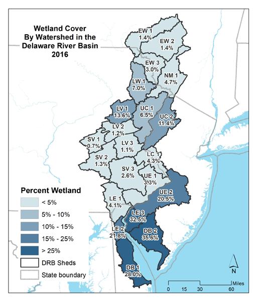
The proportion of wetlands across the Delaware Estuary and Basin varies greatly by region and watershed (Fig 6.1). The Bay Region has the greatest proportion of wetlands (~22-36%) due to the expansive tracts of salt and brackish tidal wetlands in the Estuary. In the Lower region, where development is greatest within the Estuary and Basin, however, wetland cover is substantially less. Wetland cover is often <5% of the watersheds in southeastern PA, surrounding Philadelphia. Wetland cover is closer to 20% in southwestern NJ, where there is more suburbia as well as protections provided within the Pinelands area along the eastern edge of the UE2 watershed. Wetland cover ranges from ~6-13% in the Central Region and ~15% in the Upper Region, where wetland cover on the landscape is restricted due to elevation gradients within mountainous terrain.
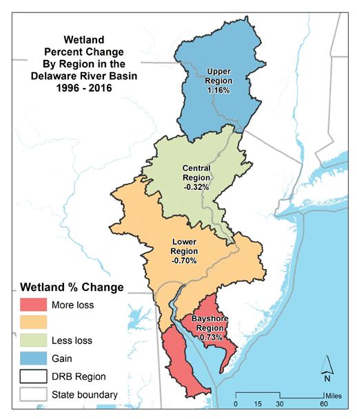
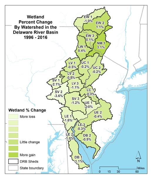
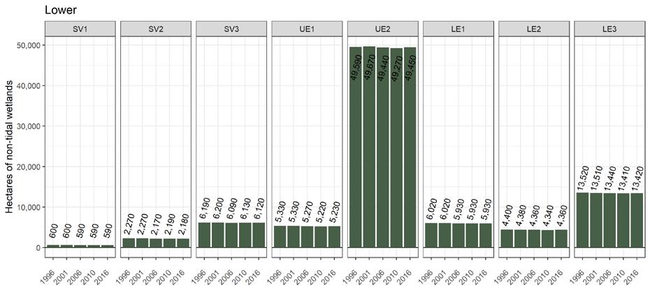
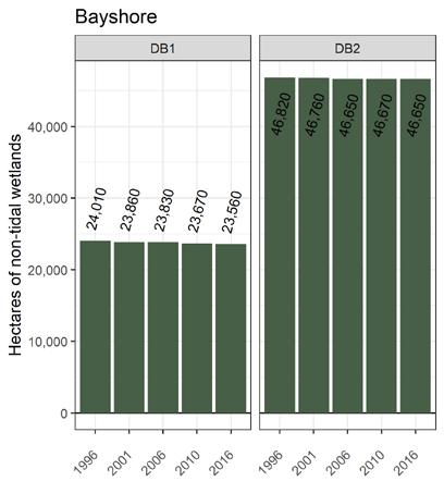
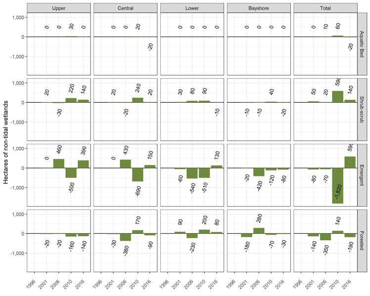
On average from 1996-2016, the Lower Region experienced the greatest loss of wetland cover (-6.4%), followed by the Bay (-4.2%) and Central Regions (-2.7%) (Fig 6.2). The Upper Region experienced wetland cover gains (+6.2%). At the watershed scale, proportional wetland losses were greatest in the most developed watersheds, such as UE1, SV 3, and LE1, and especially in SV 2, which has intensifying development and agriculture (Chapter 1) (Fig 6.3). Wetland losses in the Bay Region were higher in Delaware (-1% for LE 2 and DB 1) than losses in New Jersey (~-0.4% for LE 3 and DB 2), perhaps due to greater increase in development in those areas of Delaware (>20%) compared to New Jersey (<20%).
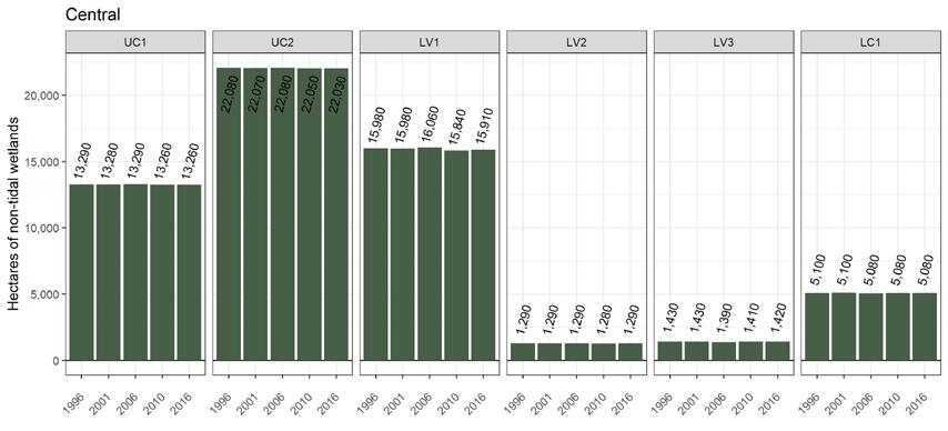
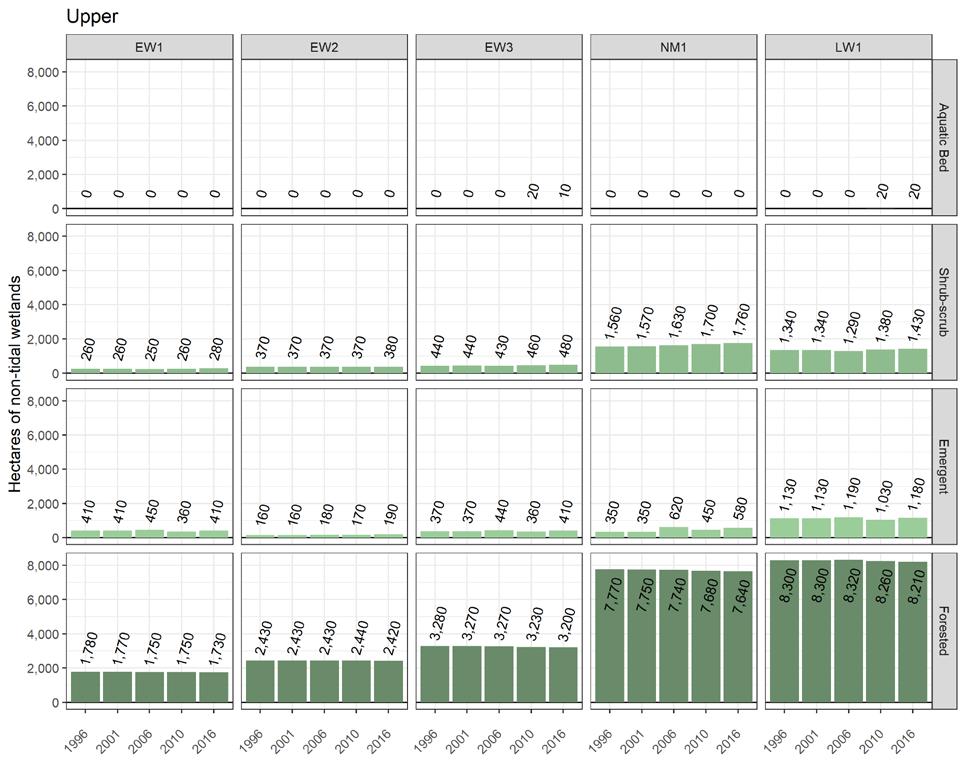
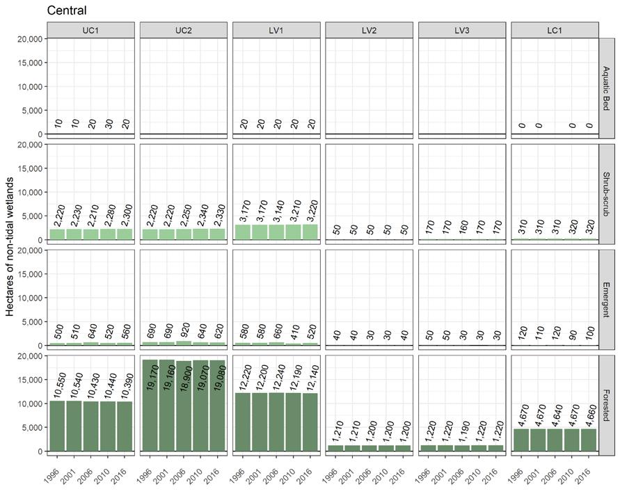
NM 1 and EW 2 had notable wetland gains, although the mechanisms for these gains are unclear. It is possible that, with increasing development in these areas, stormwater pond creation could have an observable net effect on wetland cover, especially as wetland cover in those areas is naturally low—but this is highly speculative. In other areas with increasing development, like UC 1 and UC 2, where natural wetland cover is higher than NM 1 and EW 2, stormwater ponds gains may offset only a fraction of losses. Understanding the spatiotemporal patterns of stormwater pond creation is a critical need within the Delaware Estuary and Basin, and a need that is further described in the non-tidal wetland section of this chapter.
6.1
cover by watershed in the Delaware Estuary and Basin, 2016.
6.2 Wetland cover change by region in the Delaware Estuary and Basin, 1996-2016.
6.3 Wetland cover change by watershed in the Delaware Estuary and Basin, 1996-2016.
Technical Report for the Delaware Estuary and Basin Partnership for the Delaware Estuary— Host of the Delaware Estuary Program
Figure
Wetland
Figure
Figure
6.3.1 Tidal Wetland Cover
Abstract
Tidal wetlands are likely some of the most ecologically and economically important natural habitats. Data from the National Wetlands Inventory suggests that there are 125,447 hectares (309,986 acres) of tidal wetlands in the Delaware Estuary, which is ~8% of the total land area of the Estuary. More than half of the tidal wetlands in the Delaware Estuary are salt/brackish marshes (59%), with freshwater tidal marshes covering <5%. Between 1996–2016, however, tidal wetlands of the Delaware Estuary experienced a net decline of 340 hectares (840 acres), which is an average loss of 17 hectares (42 acres or 0.56%) per year, as NOAA C-CAP data suggested. Future projections imply that these losses will likely increase due to existing degradation and accelerating sea level rise, especially if robust intervention measures are not undertaken. Research, monitoring, proactive management, and on-the-ground actions are urgently needed to minimize ongoing losses.
Introduction
Tidal wetlands are vegetated aquatic habitats which occur in the intertidal zone between open water and upland areas not regularly exposed to tidal flooding. Tidal wetlands are among the most productive habitats in the world and are critical components of the interaction between land and water in the Estuary. They perform a wide variety of vital ecosystem services, such as protecting inland areas from tidal and storm damage; storing water, carbon, and other nutrients; providing important habitat to a wide variety of wildlife, including imperiled species of birds; filtering and storing contaminants to sustain water quality; providing spawning and nursery habitat for commercial fisheries; and supporting active and passive recreation and aesthetic value. Tidal wetlands are therefore regarded as the most critical habitat type in the Delaware Estuary for supporting broad ecological health and good water quality. Assuring that tidal wetlands remain intact and continue to provide these critical functions is therefore fundamental to the overall good quality of the Delaware Estuary and Basin as a whole.
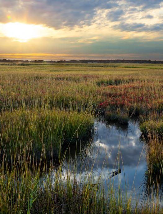
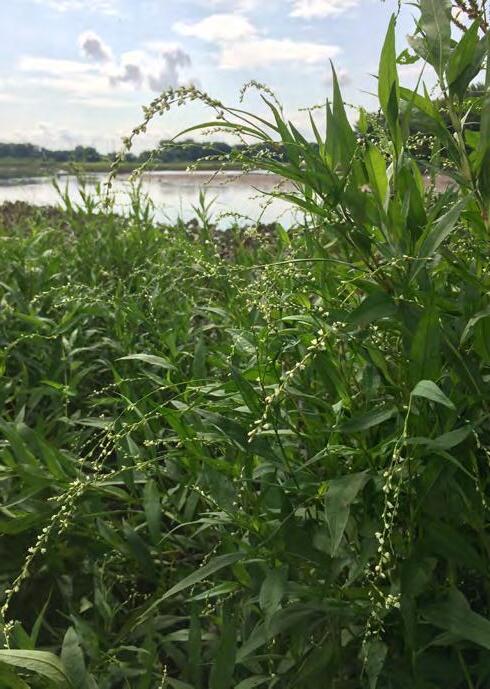
Tidal wetlands occur within the tidal extent of the Delaware Estuary, spanning a broad salinity gradient from the head-of-tide near Trenton, New Jersey, down to the mouth of Delaware Bay at Cape May, New Jersey, and Cape Henlopen, Delaware. This area is contained within the Bay (DB1, DB2) as well as the Upper (UE1, UE2) and Lower Estuary (LE1, LE2, LE3) subregions of the Estuary region of the Delaware Estuary and Basin. In the Delaware Estuary, the largest portion of tidal wetlands are the salt marshes that fringe the Delaware Bay. These tidal wetlands are mostly salt marshes, dominated by smooth cordgrass (Spartina alterniflora), with some areas mixed with salt hay (Spartina patens) and salt grass (Distichlis spicata) (Fig 6.3.1A). In the upper stretches of many tidal creeks, nationally rare communities of freshwater tidal vegetation can be dominant wherever salt concentrations are below 3 ppt (Fig 6.3.1B). Upstream of the salt line (a location where water salinities average 0.25 ppt) and within tidal reaches, the Delaware River and its tributaries support fringing and expansive freshwater tidal wetlands in the Lower and Upper Estuary regions. These freshwater tidal wetlands mainly consist of marshes dominated by perennial grasses, sedges and rushes, but there are some scrub/shrub and forested tidal wetlands as well. Typically, freshwater tidal wetlands contain a greater number of species than salt marshes; a few diagnostic species are annual wild rice (Zizania aquatica), cattails (Typha sp.), dotted smartweed (Polygonum punctatum) and forbs such as spatterdock (Nuphar advena), wapato (Sagittaria latifolia) and tuckahoe (Peltandra virginica).
A. B.
Description of Indicator
In considering tidal wetland habitats one of the leading environmental indicators for the Estuary and Basin as a whole, the science and management community of the Delaware Estuary and Basin elevated tidal wetland extent as a top priority for monitoring and management (Kreeger et al. 2006). In this chapter, landscape-level data are synthesized to assess our best current understanding of tidal wetland composition in the Estuary, as well as understanding how extent varied over space and time. This landscape-level analysis also represents Tier 1 of the Mid Atlantic Coastal Wetland Assessment (MACWA), which is a multi-tiered, multi-partner program that coordinates research and assessment of coastal wetlands in the region (see Wetlands Feature 1- Mid-Atlantic Coastal Wetland Asssessment).
Methods
Status
National Wetlands Inventory: Data on wetland distribution were gathered for each state from the U.S. Fish and Wildlife Service (USFWS) National Wetlands Inventory (NWI). The NWI is a nationwide program that inventories wetlands of the United States through aerial imagery interpretation and ground-truthing. The NWI provides detailed, consistent, high resolution data that enables differentiation of wetland types; however, it is of limited value in trend analyses for the whole system because of the different times that data are collected in different states and areas. For instance, the latest NWI data in New Jersey are from
Figure 6.3.1 Tidal wetlands in the Delaware Estuary span a salinity gradient, which includes salt marsh (A) and freshwater tidal marsh (B).
Photo by Hillel Brandes
Photo by LeeAnn Haaf
approximately 2007, 2017 in Delaware, and 2015 in Pennsylvania. Although other mapping efforts have been carried out for the general region (e.g., Carr et al. 2018; Correll et al. 2019), NWI remains the most routinely assessed and updated wetland dataset for the entire Delaware Estuary.
To determine the current extent of the various types of tidal wetlands in the Estuary, the latest of each of three state-wide NWI wetlands were used. Wetland types were categorized using the classification scheme developed by Cowardin (Cowardin et al. 1979). A simplified classification was developed to allow for a synoptic assessment of status of broad categories of wetlands within the Estuary, with special attention to the differentiation of freshwater tidal and saltwater wetlands (Fig 6.3.2). Generally, tidal wetlands were classified as forest, shrub-scrub, emergent (both estuarine marsh and freshwater tidal marsh), riverine, lake, unconsolidated, and aquatic bed. Freshwater tidal wetlands were determined by isolating palustrine wetlands with tidal flood classifications (freshwater tidal flood classifications of S, R, V, and T), which served as the freshwater tidal footprint of the Estuary.
Trends
Coastal Change Analysis Program Determining landscape level changes in different wetland types of the Delaware Estuary requires consistent data in both space and time. Since NWI lacks temporal consistency, wetlands data were derived from the National Oceanic and Atmospheric Administration’s (NOAA) Office of Coastal Management Coastal Change Analysis Program (C-CAP) datasets. These data are derived from Landsat imagery at a 30m ground resolution and are routinely assessed in 4–6 (typically 5) year intervals. Years for the C-CAP land cover data for the Delaware Estuary and Basin are 1996, 2001, 2006, 2010, and 2016.
C-CAP data are most useful for trend analyses as they are not as resolved as NWI (C-CAP is assessed at the 1:100,000 scale, whereas NWI are assessed at the 1:24,000), and may have larger classification errors. Previous assessment of the comparability of the wetland categories of the C-CAP land cover data with NWI indicates that the data are comparable to a relatively small percentage difference, particularly for salt/brackish wetlands (i.e., estuarine emergent) wetlands. As with NWI, accuracy/precision issues among various mapping methods have been noted (Weis et al. 2021), yet C-CAP remains the most methodologically consistent dataset for temporal trend analysis of wetlands for the entire Delaware Estuary. Therefore, C-CAP data were used to assess the Trends in tidal wetlands for this report, whereas NWI data were used to determine Status.
Categories of wetlands distinguished by the C-CAP are: Palustrine Forested, Palustrine Scrub/Shrub, Palustrine Emergent, Estuarine Forested, Estuarine Scrub/Shrub, Estuarine Emergent, Unconsolidated Shore, and Palustrine Aquatic Bed. Here, classifications beginning with Estuarine are considered salt or brackish tidal wetlands. At approximately the salt front, classifications consist of Palustrine categories, even though freshwater tidal marshes exist within this corridor. Therefore, the freshwater tidal footprint derived from NWI data was used to further isolate freshwater tidal wetlands for C-CAP trend analysis.
Results
Status
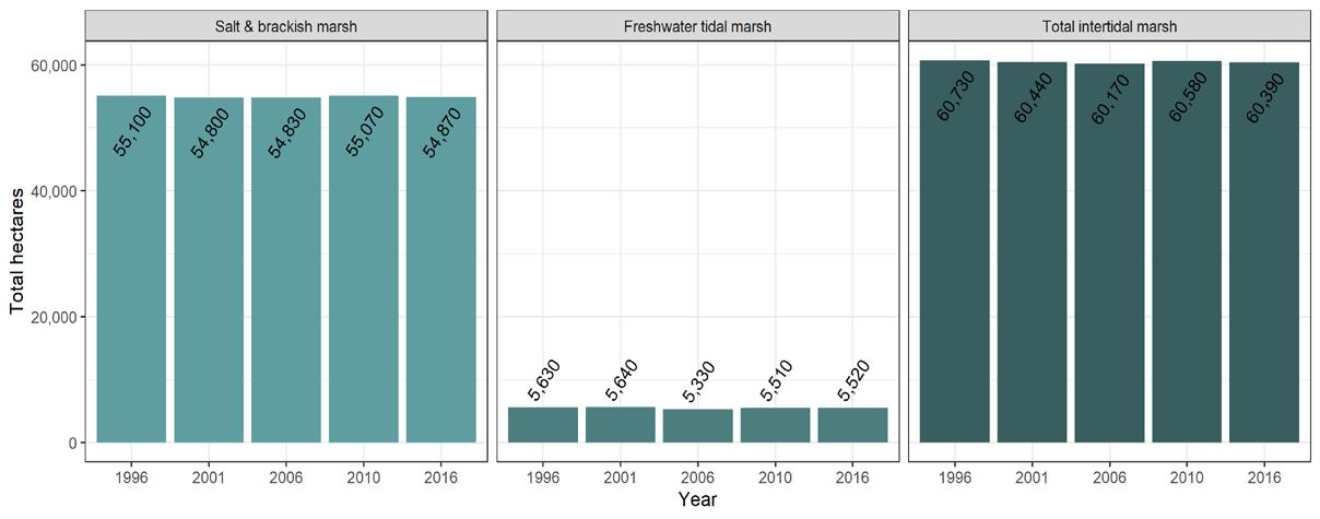
Tidal wetlands (freshwater tidal, brackish, and saline) cover 125,447 hectares (309,986 acres), which is about 8% of the total land area of the Estuary (~1.6 million hectares) (Fig 6.3.4). This is comparatively higher than the national figure of 5.5% area of wetlands in the contiguous U.S. (Dahl 2011). Emergent salt and brackish marshes account for 59% (73,390 hectares or 181,351 acres) and freshwater tidal marshes account for 4.5% (5,630 hectares or 13,912 acres) of all tidal wetlands in the Estuary. Intertidal and subtidal unconsolidated habitats (beaches, shorelines, mudflats) are 20% of tidal wetlands in the Estuary (24,730 hectares or 61,109 acres), while the remaining 16.5% of tidal habitats consist of tidal forested and shrub-
Legend
Subtype
Estuarine, Aquatic Bed
Estuarine, Forest
Estuarine, Marsh
Estuarine, Shrub-scrub
Estuarine, Unconsolidated
Freshwater tidal, Aquatic bed
Freshwater tidal, Forest
Freshwater tidal, Open water
Freshwater tidal, Marsh
Freshwater tidal, Shrub-scrub
Freshwater tidal, Unconsolidated
30 Kilometers
Figure 6.3.2 Tidal wetland cover in the Delaware Estuary based on the most recent NWI data.
Legend
Salt & brackish wetlands
Freshwater tidal wetlands
30 Kilometers
Figure 6.3.3 Tidal wetland cover in the Delaware Estuary based on 2016 NOAA C-CAP data.
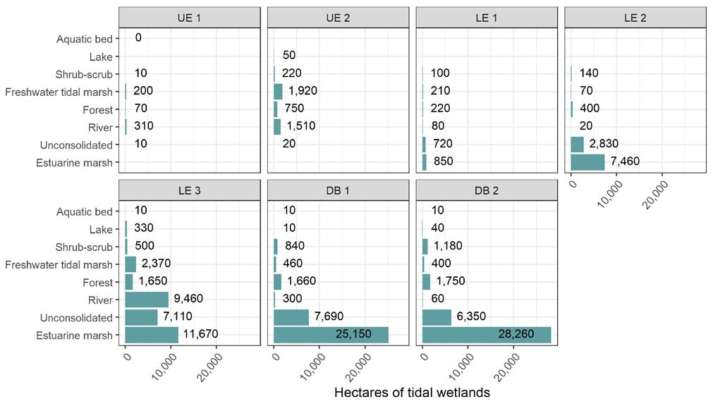
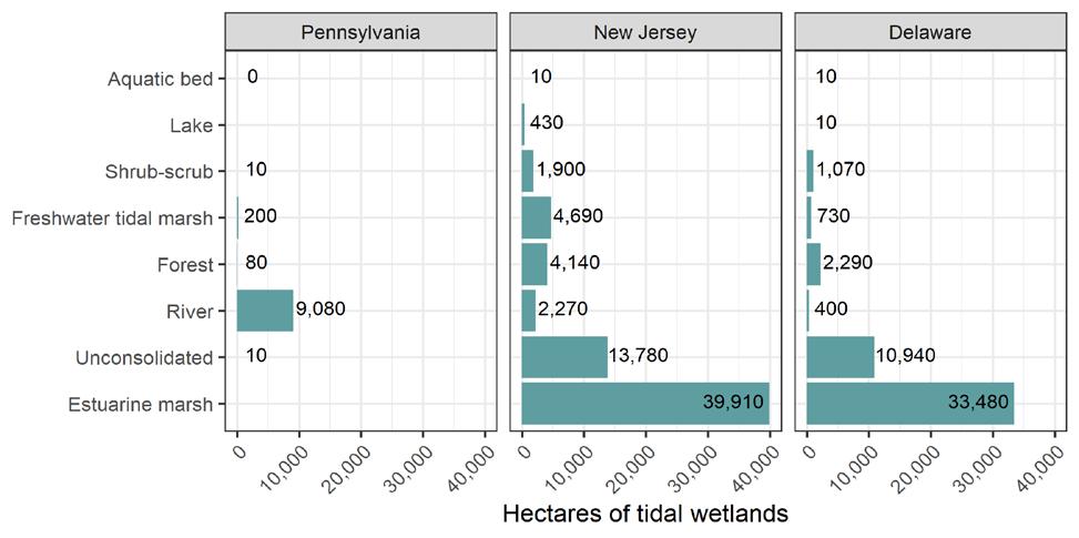
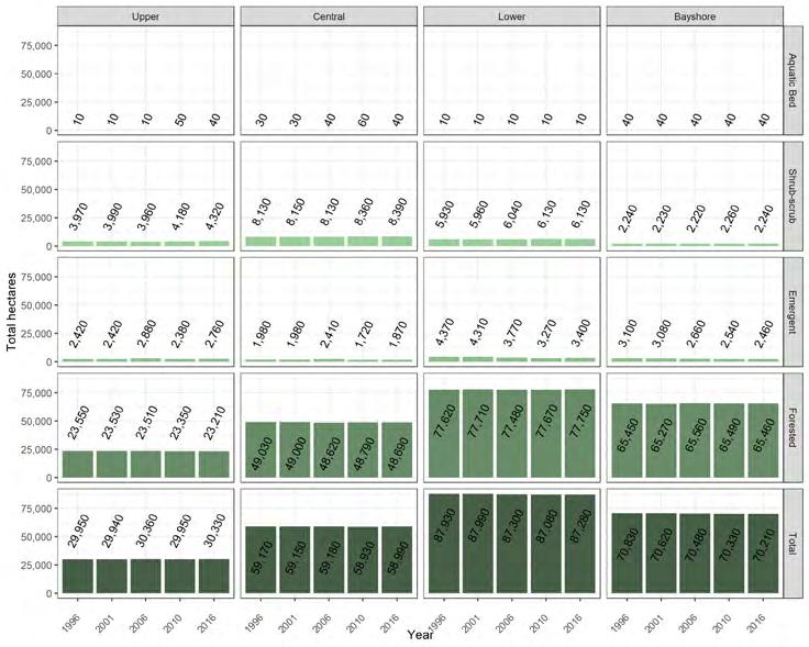
scrub habitats. In the following figures, summary information on tidal wetland acreage based on the latest NWI data was divided by subregion (Fig 6.3.4, Tables 6.3.1-6.3.2) and state (PA, NJ, and DE; Fig 6.3.5, Table 6.3.3).
Figure 6.3.4 Tidal wetland cover (in hectares) of tidal wetland types by region based on NWI classifications.
Trends
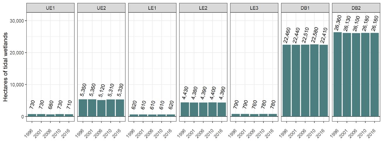
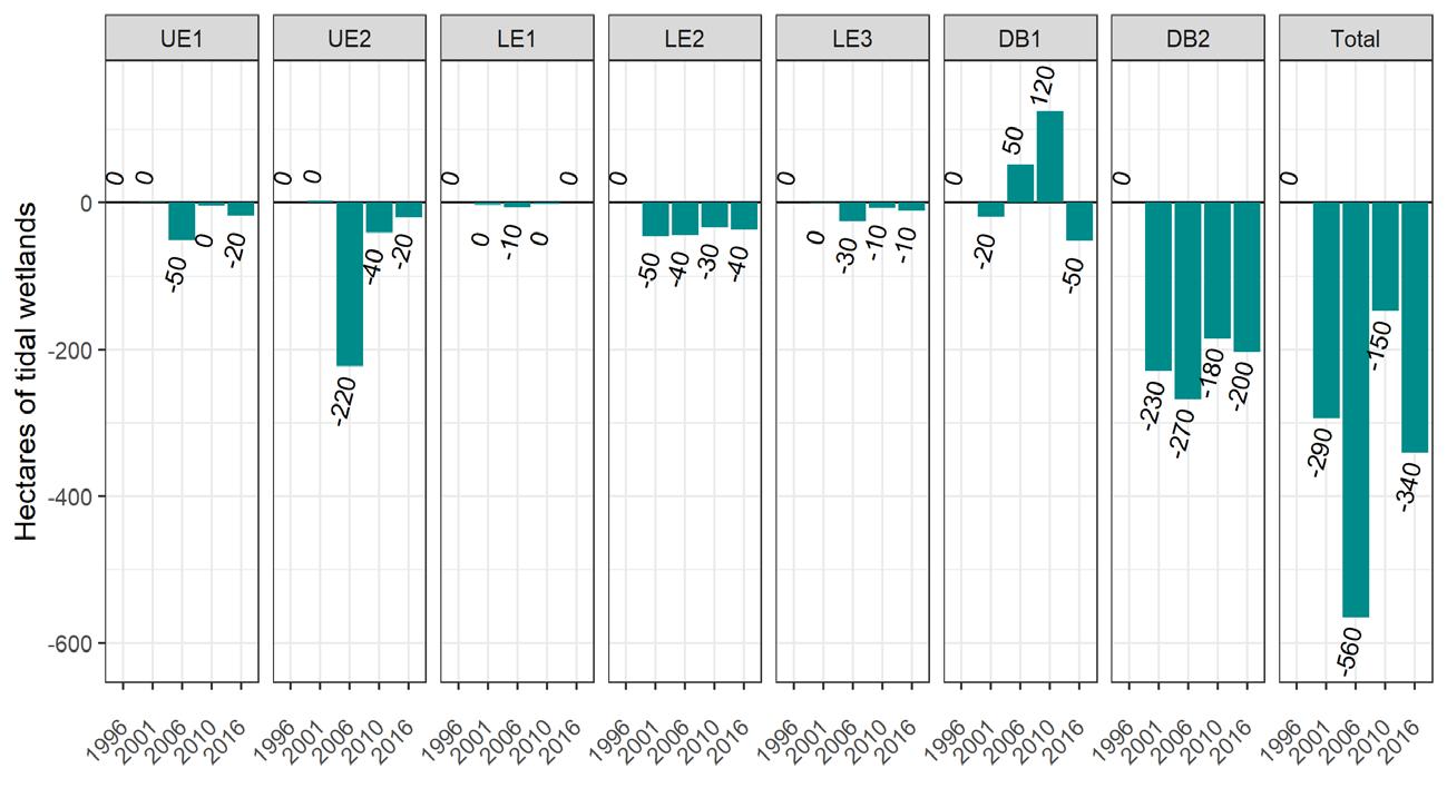
Between 1996–2016, tidal wetlands of the Delaware Estuary experienced a net decline of 340 hectares (840 acres), which is an average decline of 17 hectares (42 acres or 0.56%) per year (Figs 6.3.6-6.3.8; Table 6.3.4). The largest areas of loss were in the New Jersey Bayshore (DB2), which saw a decrease of 354 hectares (501 acres), and Delaware Bayshore (DB1), which saw a decrease of 52 hectares (128 acres). Freshwater tidal wetlands in the Upper Estuary, as well as portions of the Lower Estuary, also experienced declines ranging from 11 to 37 hectares (27–91 acres). Net change from 1996–2016 showed a very small increase (0.18 hectare or 0.44 acre) in tidal wetland acreage in subregion LE1, in northern Delaware. Although losses in the upper estuary add up to smaller acreage, losses are proportionately larger; for instance, a loss of 17 hectares from 1996–2016 in UE1 translates to a 2.4% average annual decline, whereas 203 hectares lost is a <1% average annual decline for DB2.
Freshwater tidal wetland losses totaled 1,023 hectares (2,528 acres) between 1996–2016 in the Estuary, which were mostly driven by conversion to development, open space/agriculture/grasslands, and forest/ shrub-scrub habitats (Table 6.3.5). These losses were countered by 506 hectares (875 acres) of freshwater tidal wetland gains, which were driven mostly by conversion from open water, bare or unconsolidate land, and forest/shrub-scrub habitats. Brackish/salt wetland losses in the Estuary totaled 568 hectares (1,404 acres), which were driven by conversion to open water and unconsolidated/bare land (Tables 6.3.3, 6.3.4). These losses were countered by 341 hectares (843 acres) of gains, which were driven by conversion from open water and non-tidal wetlands. Taken together, there was a net loss of 509 hectares (1,258 acres) of freshwater tidal wetlands and 226 hectares (558 acres) of brackish/salt wetland in the Delaware Estuary during the twenty year study period.
Table 6.3.1 Cover of tidal wetlands in the Delaware Estuary in the Lower Region based on NWI data.
1
1
2
3
Table 6.3.2 Cover of tidal wetlands in the Delaware Estuary in the Bay Region based on NWI data.
Figure 6.3.5 Tidal wetland cover (in hectares) of tidal wetland types by state based on NWI classifications.
Table 6.3.3 Cover of tidal wetlands in the Delaware Estuary by state based on NWI data.
Figure 6.3.6 Total tidal wetland cover in the Estuary over time by subregion
Figure 6.3.7 Total tidal wetland cover in the Estuary over time by type.
6.3.8
cover changes relative to the 1996 baseline.
Figure
Tidal wetland
Table 6.3.4 Tidal wetland cover change from 1996-2016.
Table 6.3.5 Conversions of tidal wetlands from 1996 to 2016.
Discussion
Tidal wetlands were historically lost in the Delaware Estuary primarily through their reclamation for agriculture and other purposes. Carr et al. (2018) estimated that the Delaware Estuary might have lost 22,400 hectares (55,352 acres) of tidal wetlands from 1776 to 2011. The most extensive losses occurred mostly before 1950. Direct losses of wetlands have slowed since ~1975, likely due to protections afforded by provisions in the 1972 Clean Water Act. Since 2000, total tidal wetland acreage has oscillated between approximately 60,000 and 70,000 hectares (148,000-173,000 acres) (Carr et al. 2018; this study).
As no other habitat types rival tidal wetlands in productivity, the net loss of ecosystem services are disproportionately large compared to acreage losses. Although interannual variability exists and some gains can be noted, all tidal wetland acreage losses are nevertheless impactful considering their benefits to people, fish and wildlife, and water quality. Historical and current human-mediated disturbances on estuarine systems are considerable, and development pressures are likely to continue to increase (see Chapter 1). These stressors are additionally exacerbated by climate change and sea level rise.
Mechanisms of Loss
Rising sea level is a significant contributor of tidal wetland decline in the Delaware Estuary (Carr et al. 2018). Tidal wetlands naturally have the ability to keep pace with rising sea levels through feedbacks that result in the accumulation of mineral and/or organic materials. These feedbacks, however, can be outpaced when sea level rise surpasses biological and geomorphological thresholds. When outpaced, tidal wetlands drown and convert to mudflats or open water. Nationally, 96.4% of tidal wetland losses were due to conversion to open water, with about 3.5% attributable to human effects in upland areas (Stedman and Dahl 2008). This likely holds true for the Delaware Bay, as Kearney et al. (2002) and Kearney and Riter (2011) discerned through satellite imagery that marshes in the Delaware Bay had decreasing vegetative cover and increasing proportions of open water over time. Coastal managers in Delaware and New Jersey also report rapidly expanding interior open water in the Delaware Estuary.
Anthropogenic stressors have contributed directly to degradation of tidal wetlands and, therefore, have likely contributed to their losses in the Delaware Estuary. Degradated tidal wetlands are less resilient to perturbations or stressors, and more likely to erode, drown, and deteriorate on short time scales. Coastal wetland stressors include a mix of practices such as mosquito control ditching, continued incremental filling, lack of regulatory oversight, regulatory loopholes for developers, shoreline hardening, hydrological alterations such as dredging, and pollution. Hydrological alterations, fill, diking, ditching, among numerous other stressors, have been directly observed from on-the-ground inventories of tidal wetland conditions in the Delaware Estuary (see Mid Atlantic Tidal Rapid Assessment reports). Historical diking for salt hay farming has led to low relative elevations of many tidal wetlands in New Jersey, which decreases their resilience to sea level rise and increases the probability that they convert to open water. As a result, ~3,600 hectares of New Jersey salt marsh (in LE3, DB2) converted to open water as a direct result of historical diking from 1931 to 2017 (Smith et al. 2017). Kearney et al. (2002) also found that more than two-thirds of the salt marshes studied in both the Chesapeake and Delaware Bays were in degraded condition. Additionally, nutrient loading might reduce the need for ample below ground production, potentially impairing a marsh’s ability to keep pace with sea level rise (Deegan et al. 2012).
Tidal marshes need ample sediment supplies to keep pace with sea level, so regional sediment management is also a concern for tidal marsh sustainability in the Delaware Estuary. The Delaware Estuary is a naturally muddy system, but more sediments are removed each year through maintenance dredging than enter the system through surface runoff. The overall budget (inputs and outputs of sediments at the Estuary scale) appears to be in balance despite regular sediment removal during channel dredging, and so, it is likely that the budget is subsidized by inputs of sediments from eroding or disintegrating tidal wetlands (Delaware Estuary Regional Sediment Management Plan 2013). Sediment management in the
Estuary should continue to consider how to retain sediment within the system, such as through thin layer placement or other types of beneficial reuse of dredged materials, in order to provide tidal wetlands the provisions they need to keep pace with rising sea levels and compensate for, or mitigate, erosional losses.
Prognosis
The rate of relative sea level rise (SLR) is critically important for determining the fate of tidal wetlands in the Delaware Estuary. SLR is currently estimated between 4-5 mm/yr in the Delaware Estuary (see Chapter 2). The upper threshold of SLR at which tidal marshes can build vertically, however, is about 10 mm/yr (D’Alpaos et al. 2011). SLR is likely to rise ~1.5 meters from 2000 to 2100 under high carbon dioxide emissions, which averages approximately 15 mm/yr (Callahan et al. 2017; Kopp et al. 2019). A new NOAA report further suggests that, under a high emissions scenario, the Northeastern U.S. may see 0.54 m of rise between 2000 and 2050 (~10.8 mm/yr), but rise might exceed 2 m from 2000 to 2100 (20 mm/yr) (Sweet et al. 2022). These sea level rise projections suggest that the limit at which tidal marshes can keep pace with SLR will likely be breached before 2100 unless significant actions are taken to aid the vertical accretion and migration of tidal wetlands.
As sea levels rise and thresholds are reached, declines in tidal wetland acreage are expected. Based on Sea Level Affecting Marsh Model (SLAMM, V.6) predictions for 2100 with 1 m of SLR, a net loss of 18,000 hectares of tidal wetlands were predicted (Kassakian et al. 2017). As the Estuary has approximately 125,000 hectares of tidal wetlands based on NWI data, this would be about a 14% loss. Other recent SLAMM modeling of focal Delaware Bay salt marshes suggest that total marsh gains might first increase, subsidized by the expansion of regularly flooded areas, until thresholds in SLR are reached (between 0.81.0 m of SLR). Thereafter, total declines are likely to become evident (Stamp et al. 2019).
As these SLAMM runs were augmented using on-the-ground data from MACWA efforts, it is apparent that site-specific tidal wetland conditions play critical roles in the sustainability of tidal wetlands with continued, and likely accelerating, SLR (Stamp et al. 2019). In a linear model analysis of tidal wetland acreage trends relative to sea level, Carr et al. (2018) found that for every 1 cm rise in sea level, wetland area historically declined by 169 hectares (418 acres). Given current rates of SLR (~5 mm/yr), 169 hectares would be lost every 20 years. However, C-CAP data here suggests that 340 hectares of tidal wetlands have been lost in the 20 years from 1996 to 2016. Sea level rise acceleration in combination with degraded conditions, driven human disturbances in 19th and/or 20th centuries, have likely contributed to these additional losses.
Climatic changes, such as warming temperatures and altered precipitation patterns, will also likely affect tidal wetland extent in the Delaware Estuary (see Chapter 2). On one hand, a longer growing season and warmer temperatures likely will increase total tidal marsh productivity (Kirwan et al. 2009). Warming trends are also expected to increase the incidence and intensity of coastal storms, including nor’easters and hurricanes. Storm-related damages to tidal wetlands, such as excessive erosion, submergence, and salt intrusion could exacerbate other threats and stressors mentioned above. Storms may provide pulses of sediment to tidal wetlands that help them build vertically, but damages may outweigh benefits, especially in already degraded or fragmented wetlands.
Moreover, tidal wetlands face barriers to landward migration within the Delaware Estuary. The potential for tidal wetlands to migrate landward is affected by slope, soils, degree of development, and other ecological considerations (such as upland habitat plant community composition). Areas that do not allow tidal wetlands to migrate landward must accrete in place and stave off excessive erosion to preserve acreage or drown. Despite that forest conversion to marsh is a leading hypothesis of future salt marsh gains, C-CAP data in the Delaware Estuary suggested that no salt/brackish marsh net gains were caused
directly by upland forest conversion. However, ongoing research in the Delaware Estuary has found that forested areas in the region are indeed converting to salt marshes as sea levels rise (Smith 2013; Sacatelli et al. 2020; Feature 2 - Coastal Forest Die Back). In this report, gains appeared to be most notably driven by the conversion of open water and non-tidal wetlands, which also includes forested wetlands (this study; Osland et al. 2022). Patterns of non-tidal wetland conversion, emergent and forested, will therefore be an important area of additional consideration and research. More research on processes that drive marsh migration is needed to help support planning for coastal land use adaptations as rising sea levels and tidal wetland losses cause land cover transitions.
Actions and Needs
Sea level rise, salinity intrusion, anthropogenic disturbance, outdated management paradigms, and pollutants will likely continue to contribute to degradation and loss of tidal wetlands in the Delaware Estuary unless very swift actions are taken to abate these impacts. Managers should carefully consider how a projected loss of tidal wetlands in the Delaware Estuary might affect coastal communities (lives and property) and regional economies (fisheries and shellfisheries, property values, nutrient criteria for industry). The following are actions and needs to aid efforts to reduce tidal wetland losses:
Proactive Adaptive Management
Despite the dynamic nature of the coastline, many regulatory policies continue to treat the landscape as fixed in place. Restoration paradigms set goals based on historic conditions rather than future sustainability. It is generally still easier to obtain a permit for a bulkhead or other hard structures, which can contribute to degradation of tidal wetlands, than it is for a living shoreline. The state of Delaware had taken a lead in making living shoreline permitting and construction easier, and is now being followed by New Jersey and Pennsylvania. Ditching, diking, excavating, and filling of tidal wetlands still occur, often without a good understanding or monitoring of the consequences. New active policies and tactics are needed to both facilitate the horizontal migration and vertical accretion of tidal marshes. Marsh migration management plans are needed and will require conflict resolution and education. To adapt to both climate change and continued watershed development, tidal wetland managers and landowners will need to adjust targets, expectations, and tactics to sustain the most tidal wetland habitat in the future.
In order to address threats to tidal wetlands in Delaware Estuary, an approach combining policy and regulatory remedies and actions on the ground is still needed. The 1972 Clean Water Act, the 1972 Coastal Zone Management Act, and the 1982 Coastal Barriers Resources Act, are evidence of the importance of tidal wetlands in the policy and legal arena. Many states and counties have followed the lead of federal agencies and implemented their own regulations covering such wetland protection measures as buffer requirements, impervious cover limitations, and implementation of federal National Pollutant Discharge Elimination System (NPDES) and total maximum daily load (TMDL) guidelines.
Continued promulgation and refinement of regulations and policies is a critical need, as demonstrated by the various emergency measures that are already underway or being called for in some Delaware and New Jersey areas (e.g. Prime Hook, Delaware; Sea Breeze, New Jersey; Maurice Township, New Jersey) where tidal wetland losses are contributing to the decline of coastal communities. Given accelerating development and population pressures, as well as increases in relative sea level rise and climate change, these measures will need to be augmented to maintain the current integrity of the tidal wetlands. In particular, local differences in the extent of regulatory protection for wetlands poses a challenge to maintaining consistently high levels of wetland quality and function in the Estuary.
Continued Monitoring and Scientific Study
Another need for protecting tidal wetland extent is continued and complete data on their current conditions, as well as scientific information on factors that drive losses and best management practices
to avert such losses. Although monitoring efforts have been underway through MACWA efforts (Feature 1 - Mid-Atlantic Coastal Wetland Assessment), the synthesis and continued support of these programs is critical in understanding the complexities that affect tidal wetland condition, extent, and sustainability into the future. These data are also useful for prioritizing and planning intervention strategies across the Estuary.
Investment in tidal marsh monitoring and science is difficult to fund at the multi-state scale of the Delaware Estuary. However, the benefits of tidal wetlands are beginning to be captured and capitalized (e.g. flood protection, nutrient and carbon capture, fish production; see Feature 3 - Blue Carbon). As markets for ecosystem services develop in the future, there could be increasing demand for essential information on trends in tidal wetland extent and condition, as well as tactics to protect and enhance tidal wetlands. However, until markets evolve that can generate needed resources to sustain monitoring and assessment there will continue to be a need to collaborate and leverage funds to fill vital information gaps.
On-the-ground Action
Given the rapid pace of change in tidal wetland extent and health, swift action to physically protect or enhance tidal wetlands is warranted to stem losses even if monitoring and scientific information are still developing. Seaward protections and marsh enhancements can be difficult to implement due to permitting, logistical and funding challenges. However, there are efforts to explore beneficial use of sediments for enhancement (Delaware Estuary Regional Sediment Management 2013), develop new types of hybrid living shorelines and craft estuary-wide strategies for intervention implementation (e.g., Delaware Estuary Living Shoreline Initiative).
New prioritization and decision-making tools are becoming available to facilitate the design and implementation of invention projects using on-the-ground data, which will improve success rates. In the Delaware Estuary, these tools include New Jersey Coastal Resilience Collaborative Prioritization Tool, the New Jersey Coastal Ecological Restoration and Adaptation Plan, as well as the Living Shoreline Feasibility Model, the Wetland Assessment Tool for Condition and Health, and Marsh Futures.
References
Callahan, John A., Benjamin P. Horton, Daria L. Nikitina, Christopher K. Sommerfield, Thomas E. McKenna, and Danielle Swallow. 2017. Recommendation of Sea-Level Rise Planning Scenarios for Delaware: Technical Report, prepared for Delaware Department of Natural Resources and Environmental Control (DNREC) Delaware Coastal Programs.
Carr, Edward W., Yosef Shirazi, George R. Parsons, Porter Hoagland, and Christopher K. Sommerfield. 2018. Modeling the Economic Value of Blue Carbon in Delaware Estuary Wetlands: Historic Estimates and Future Projections. Journal of Environmental Management 206: 40–50. https://doi. org/10.1016/j.jenvman.2017.10.018.
Correll, Maureen D., Wouter Hantson, Thomas P. Hodgman, Brittany B. Cline, Chris S. Elphick, W. Gregory Shriver, Elizabeth L. Tymkiw, and Brian J. Olsen. 2019. Fine-Scale Mapping of Coastal Plant Communities in the Northeastern USA. Wetlands 39. Wetlands: 17–28. https://doi. org/10.1007/s13157-018-1028-3.
Cowardin, Lewis M., Virginia Carter, Francis C. Golet, and Edward T. LaRoe. 1979. Classification of wetlands and deepwater habitats of the United States. FGDC-STD-004-2013. Second Edition. https://doi.org/FWS/OBS-79/31.
D’Alpaos, Andrea, S. M. Mudd, and Luca Carniello. 2011. Dynamic response of marshes to perturbations in suspended sediment concentrations and rates of relative sea level rise. Journal of Geophysical Research: Earth Surface 116: 1–13. https://doi.org/10.1029/2011JF002093.
Dahl, T.E. 2011. Status and Trends of Wetlands in the Conterminous United States 2004 to 2009. U.S. Department of the Interior; Fish and Wildlife Service, Washington, D.C.: 108.
Deegan, Linda a., David Samuel Johnson, R. Scott Warren, Bruce J. Peterson, John W. Fleeger, Sergio Fagherazzi, and Wilfred M. Wollheim. 2012. Coastal eutrophication as a driver of salt marsh loss. Nature 490: 388–392. https://doi.org/10.1038/nature11533.
Delaware Estuary Regional Sediment Management Plan (DERSMP). 2013. Prepared by the Delaware Estuary Regional Sediment Management Plan Workgroup. http://www.nj.gov/drbc/library/ documents/RSMPaug-2013final-report.pdf
Kassakian, Jennifer, Ann Jones, Jeremy Martinich, and Daniel Hudgens. 2017. Managing for No Net Loss of Ecological Services: An Approach for Quantifying Loss of Coastal Wetlands due to Sea Level Rise. Environmental Management. Springer US: 0–1. https://doi.org/10.1007/s00267-0160813-0.
Kearney, Michael S., and J. C. Alexis Riter. 2011. Inter-annual variability in Delaware Bay brackish marsh vegetation, USA. Wetlands Ecology and Management 19: 373–388. https://doi.org/10.1007/ s11273-011-9222-6.
Kearney, Michael S., Andrew S. Rogers, John R. G. Townshend, Eric Rizzo, David Stutzer, J. Court Stevenson, and Karen Sundborg. 2002. Landsat imagery shows decline of coastal marshes in Chesapeake and Delaware Bays. Eos, Transactions American Geophysical Union 83: 173. https:// doi.org/10.1029/2002EO000112.
Kirwan, Matthew L., Glenn R. Guntenspergen, and James T. Morris. 2009. Latitudinal trends in Spartina
alterniflora productivity and the response of coastal marshes to global change. Global Change Biology 15: 1982–1989. https://doi.org/10.1111/j.1365-2486.2008.01834.x.
Kopp, R. E., C Andrews, A Broccoli, A Garner, D Kreeger, R Leichenko, N Lin, et al. 2019. New Jersey’s Rising Seas and Changing Coastal Storms: Report of the 2019 Science and Technical Advisory Panel November 2019.
Kreeger, D., R. Tudor, J. Sharp, S. Kilham, D. Soeder, M. Maxwell-Doyle, J. Kraeuter, D. Frizzera, J. Hameedi and C. Collier. 2006. White paper on the status and needs of science in the Delaware Estuary. Partnership for the Delaware Estuary, Report #06-01. 72 pp.
Osland, M.J., Chivoiu, B., Enwright, N.M., Thorne, K.M., Guntenspergen, G.R., Grace, J.B., Dale, L.L., Brooks, W., Herold, N., Day, J.W. and Sklar, F.H., 2022. Migration and transformation of coastal wetlands in response to rising seas. Science Advances, 8(26), p.eabo5174.
Sacatelli, R, R. G. Lathrop, and M Kaplan. 2020. Impacts of climate change on coastal forests in the northeast US. Rutgers University. https://doi.org/10.1007/978-3-030-32878-8_7.
Smith, Joseph A.M., Steven F. Hafner, and Lawrence J. Niles. 2017. The impact of past management practices on tidal marsh resilience to sea level rise in the Delaware Estuary. Ocean and Coastal Management 149. Elsevier Ltd: 33–41. https://doi.org/10.1016/j.ocecoaman.2017.09.010.
Smith, Joseph A M. 2013. The Role of Phragmites australis in Mediating Inland Salt Marsh Migration in a Mid-Atlantic Estuary. PLoS ONE 8. https://doi.org/10.1371/journal.pone.0065091.
Stamp, Jenifer, Anna Hamilton, Marissa Liang, Jonathan Clough, Marco Propato, LeeAnn Haaf, and Jordan West. 2019. Application of the sea-level affecting marshes model (SLAMM) to the lower Delaware Bay, with a focus on salt marsh habitat. Washington, DC.
Stedman, Susan Marie, and Thomas E Dahl. 2008. Status and Trends of Wetlands In the Coastal Watersheds of the Eastern United States 1998 to 2004: 36.
Sweet, W.V., B.D. Hamlington, R.E. Kopp, C.P. Weaver, P.L. Barnard, D. Bekaert, W. Brooks, et al. 2022. Global and Regional Sea Level Rise Scenarios for the United States. Silver Spring, MD.
Weis, Judith S., Elizabeth Burke Watson, Beth Ravit, Charles Harman, and Metthea Yepsen. 2021. The status and future of tidal marshes in new jersey faced with sea level rise. Anthropocene Coasts 4: 168–192. https://doi.org/10.1139/anc-2020-0020.
Technical Report for the Delaware Estuary and Basin Partnership for the Delaware Estuary— Host of the Delaware Estuary Program
1. Partnership for the Delaware Estuary; 2. Barnegat Bay Partnership
The Partnership for the Delaware Estuary (PDE) and the Barnegat Bay Partnership (BBP) established the Mid Atlantic Coastal Wetlands Assessment (MACWA) in 2008 to address critical knowledge gaps regarding the current conditions of coastal wetlands and future risks to these wetlands posed by climate change and sea level rise. Shortly thereafter, the Academy of Natural Sciences at Drexel University, New Jersey Department of Environmental Protection (NJDEP), and Delaware Department of Natural Resources and Environmental Control (DNREC) joined the effort. Before MACWA, no single entity had been able to consistently assess or track the extent and condition of coastal wetlands across the Delaware Estuary and Barnegat Bay. Consequently, only patchy or inconsistent data existed on coastal wetland status and trends, despite the importance of these data to decision makers. From the onset, MACWA objectives sought to develop a comprehensive coastal wetlands assessment program to establish a baseline of current conditions, perform ongoing monitoring, and conduct special studies to answer questions about the drivers of coastal wetland health and function. MACWA has continued to evolve with the help of its numerous regional partners.
For the first thirteen years of its implementation, MACWA was composed of 4 tiers, which followed the three basic tiers recommended by EPA, plus an additional tier aimed to facilitate research to answer specific questions about coastal wetland condition or function. In 2020, MACWA partners highlighted the persistent yet ever-expanding need to address education, diversity, equity, inclusion, and justice in the realm of coastal resilience. Components of MACWA already sought to engage different audiences, such as using social media to help the public appreciate the beauty of coastal wetlands, or presenting data at regional or national scientific conferences, but a need to be more intentional about reaching even broader audiences and helping rectify environmental inequities and injustices was identified. To codify this, a fifth tier of MACWA, titled Social Science and Science Communication, was proposed. The five MACWA tiers as established are:
• Tier 1 – Landscape level assessments
• Tier 2 – Rapid Assessments through the Mid Atlantic Tidal Rapid Assessment (MidTRAM)
• Tier 3 – Special research studies
• Tier 4 – Intensive monitoring through Site Specific Intensive Monitoring (SSIM)
• Tier 5 – Social Science and Science Communication
MACWA initiatives, or the sub-programs implemented to support the framework, are selected based on how methodological objectives aligned with each tier. Tier 1 assessments or those focused on determine coastal wetland extent. We have completed these studies relative to National Estuary Programs requirements to produce State of Estuary reports, like the TREB. MidTRAM, which DNREC originally developed (~2007) and has since been adopted into the MACWA framework, represents Tier 2. Tier 3 includes special studies that seek to understand specific components of coastal wetland condition and function. These studies have covered topics such as restoration project monitoring, blue carbon assessments, living shoreline monitoring, as well as sediment or dendrochronological studies. SSIM, which we first piloted in 2010, represents Tier 4. We routinely collect SSIM data at designated stations and fulfill the need for understanding long-term dynamics in coastal wetland systems.
Major findings
Tier 1 Chapter 6.2.1 in this TREB report
Tier 2 PDE, BBP, and DNREC have implemented Tier 2 rapid assessments in numerous watersheds throughout the Mid-Atlantic region (Figure 6.3.9). These assessments have provided a better understanding of wetland conditions and stress distribution on a watershed-wide scale. Land managers and restoration practitioners have used MidTRAM data to better understand stressor-response gradients, determine natural differences among different areas or marsh types, and recently to help prioritize areas for restoration potential. MidTRAM data from several watersheds in coastal New Jersey, Pennsylvania and Delaware indicate that most studied tidal wetlands had some degree of stressed condition. Most of the study areas also exhibited areas that were both severely and moderately stressed (Figure 4). The Christina River watershed had the lowest average score due to numerous instances of altered hydrology in the downstream section of the watershed. On the other hand, the Mullica Estuary is one of the least disturbed study areas and received higher final MidTRAM scores with no sites having a severely stressed final score. Data collected through MidTRAM is being included in the Penn State Riparia Database to disseminate wetland condition information to practitioners, scientists and land managers.
Tier 3 Special studies conducted through tier 3 projects have sought to address research questions related to wetland condition, function, ecosystem services, and/or restoration (Table 1). Protocols and data furnished from Tiers 1, 2 and 4 help to inform experimental design and shape the findings and conclusions of these studies. PDE and BBP are currently integrating these data into various tools to help
Figure 6.3.9 Final MidTRAM scores throughout New Jersey, Pennsylvania, and Delaware indicate stressed wetlands (yellow or red points) existed at a majority of studied watersheds. Studied watersheds are: Christina River (CHR), Red Lion Creek (RED), Barnegat Bay North (BBN), Supawna NWR (SUP), Inland Bays), Barnegat Bay South (BBS), Broadkill River (BDL), Pennsylvania Tidal (PAT), St Jones River (STJ), Mispillion River (MISP), Appoquinimink Creek (APP), Murderkill (MUR), Maurice River (MAU), Crosswicks Creek (CRW), SMyrna River (SMY), Leipsic River (LEI), Dennis Creek (DEN), Reeds Beach (DB), and the Mullica River (MULL).
prioritize areas for potential restoration. Tier 3 studies can also be conducted at the local level such as current groundwater studies in targeted priority coastal forests that are investigating the effects of saltwater intrusion and groundwater dynamics in coastal forest transition zones. For more, see PDE’s MACWA website.
Tier 4 Long term monitoring in Barnegat Bay and the Delaware Estuary has produced extensive long-term monitoring datasets, including those on water quality, soil quality, elevation, and vegetation community metrics. These datasets provide essential baseline information about how coastal wetland conditions can vary through time and in response to changing environmental conditions. Whether tidal marshes are keeping pace with rising sea level is one of the chief study questions for Tier 4 monitoring. From Tier 4 SSIM monitoring, we found that the rate of elevation change at most of these study sites does not keep pace with recent rates of sea level rise (Figure 6.3.10). This is especially true for the study sites in Delaware Bay where none of the salt marsh monitoring sites are keeping pace with the observed increase in sea level of 5.5 cm from 2011-2021. In Barnegat Bay, the West Creek/Dinner Point (WC) site saw a large increase in elevation in 2013 due to sediment side casting from Open Water Marsh Management (OMWM), a mosquito management technique.
Figure 6.3.10 Mean elevation change at long term monitoring sites in Barnegat Bay and the Delaware Estuary from 2011-2019. The dashed lines represent mean sea level (MSL) where the slope of the line is the change in sea level from the average monthly sea level in 2011 (starting point of 0) to the average monthly MSL in 2019 (give as the difference in cm). In the Delaware Estuary, freshwater tidal sites (turquoise) should be compared to the change in MSL at Philadelphia (a change of 0.68 cm), whereas the saline sites (dark blue) should be compared to MSL at Cape May (a change of 5.5 cm). Sites are West Creek (WC), Reedy Creek (RC), Horse Point (HP), Island Beach (IB) in Barnegat Bay, and Tinicum (TN), Christina River (CH), Crosswicks Creek (CW), Dividing Creek (DV), Maurice River (MR), Broadkill River (BK) and Dennis Creek (DN) in the Delaware Estuary.
Coastal Forest Dieback in the Delaware Bay
Rachael Sacatelli, Richard G. Lathrop, Marjorie Kaplan Rutgers, The State University of New Jersey
The coastal forests around the Delaware Bay are commonly a mix of deciduous hardwoods and evergreen conifers with the species composition dependent upon the site level soil moisture gradient (Anderson et al., 2013a; Butler-Leopold et al., 2018; Janowiak et al., 2018). In addition to providing protective buffering of inland areas against coastal storms (Williams et al., 2003; Barbier et al., 2011; Duarte et al., 2013), these forests provide a range of ecosystem services including carbon storage (McGarvey et al., 2015, Fahey et al., 2010), valuable timber resources, and habitat for a diversity of rare plants and animals including a number of species of concern (Global Rank G1-G4) (Anderson et al., 2013b).
Various studies have documented that these coastal forests are showing signs of stress evidenced by trees at the forest-tidal salt marsh edge dying back and the forests transitioning into tidal salt marsh ecosystems (Smith, 2013; Kirwan and Gedan, 2019; Sacatelli, 2020). These areas have been referred to as “ghost forests” denoting the presence of standing dead trees within or fringing the edge of salt marsh ecosystems (Able et al., 2018; Kirwan and Gedan, 2019; Ury et al., 2021). While this phenomenon of coastal forest dieback and replacement with salt marshes as sea level rises has been ongoing for millennia (Clark, 1986; Able 2021), there is widespread concern that accelerating local sea-level rise (Kopp et al. 2019; Gornitz et al., 2019; Boesch et al. 2018; Sweet et al., 2017b; Oppenheimer et al., 2019) and intensifying coastal storms and associated surges (Gornitz et al., 2019) may be hastening this process (Schieder and Kirwan, 2019).
The dieback of the forest ecosystem at the salt water tidal marsh edge (or marsh/forest ecotone) and transition to tidal salt marsh ecosystems is often referred to in the literature as the migration (or transgression) of the salt water tidal marsh into the coastal forest (Wasson et al. 2013, Kirwan and Gedan, 2019, Hussein, 2009; Smith, 2013; Schieder et al., 2018; Sacatelli, 2020). This coastal dieback and subsequent marsh migration for selected areas along the Delaware Bay has recently been mapped using historical aerial photography between the years 1940 and 2015 (Figure 6.3.11) (Sacatelli, 2020). The study found an average rate of coastal forest dieback was 3.2 m/yr, ranging from 0.4m/yr to 8.3m/yr depending on the location (Sacatelli, 2020). When examined in temporal increments, these rates also show evidence of accelerating in recent years (Sacatelli, 2020).
Subsequently, a Mid-Atlantic region-wide assessment has been undertaken to map those coastal forest areas vulnerable to future sea level rise. The consensus SLR estimates determined for New Jersey (https:// www.nj.gov/dep/climatechange/pdf/2019-stap-report-summary.pdf) suggest that 1 foot of SLR could be reached by 2050. This 1’ rise in sea level is estimated to put over 250,000 acres of coastal forest at risk of dieback 1’ (Lathrop et al., in prep). However, when compared with historical change analysis (described above), the results suggest that low-lying forested areas predicted to be at risk under future sea level rise are already experiencing stress and dieback at current SLR levels (Lathrop et al., in prep). We can expect that this phenomenon of ghost forests along Delaware Bay to be an ever present feature into the foreseeable future.
Figure 6.3.11 Locations of the treeline as of 1940 and 2015 at 5 sites along the New Jersey coast of the Delaware Bay. The area between the two lines is the area of forest lost between 1940 and 2015.
References
Able, K.W., J. Walker and B.P. Horton. (2018). Ghost forests in the Mullica Valley: Indicators of sea-level rise. Sojourn 2(2):87-96.
Able, K. W. (2021). From Cedar Cemeteries to Marsh Lakes: a Case Study of Sea-Level Rise and Habitat Change in a Northeastern US Salt Marsh. Estuaries and Coasts. 44. 10.1007/s12237-021-00946-x.
Anderson, C.J.; Lockaby, B.G.; Click, N. (2013a). Changes in wetland forest structure, basal growth, and composition across a tidal gradient. The American Midland Naturalist. 170(1): 1-13. https://doi. org/10.1674/0003-0031-170.1.1.
Anderson, M.G. M. Clark, C.E. Ferree, A. Jospe, A. Olivero Sheldon and K.J. Weaver. (2013b). Northeast Habitat Guides: A companion to the terrestrial and aquatic habitat maps. The Nature Conservancy, Eastern Conservation Science, Eastern Regional Office. Boston, MA. http://nature.ly/HabitatGuide
Barbier, E. B., Hacker, S. D., Kennedy, C., Koch, E. W., Stier, A. C., & Silliman, B. R. (2011). The value of estuarine and coastal ecosystem services. Ecological monographs, 81(2), 169-193.
Boesch, D. F., Boicourt, W. C., Cullather, R. I., Ezer, T., Galloway Jr, G. E., Johnson, Z. P., ... & Li, M. (2018). Sealevel rise: projections for Maryland 2018. 27 pp. University of Maryland Center for Environmental Science, Cambridge, MD.
Butler-Leopold, P. R., Iverson, L. R., Thompson, F. R., Brandt, L. A., Handler, S. D., Janowiak, M. K., ... & Clark, K. L. (2018). Mid-Atlantic forest ecosystem vulnerability assessment and synthesis: a report from the MidAtlantic Climate Change Response Framework project. Gen. Tech. Rep. NRS-181. Newtown Square, PA: US Department of Agriculture, Forest Service, Northern Research Station. 294 p., 181, 1-294.
Clark, J. S. (1986). Coastal forest tree populations in a changing environment, southeastern Long Island, New York. Ecol. Monogr. 56, 259–277. doi: 10.2307/2937077
Duarte, C. M., Losada, I. J., Hendriks, I. E., Mazarrasa, I., & Marbà, N. (2013). The role of coastal plant communities for climate change mitigation and adaptation. Nature Climate Change, 3(11), 961-968.
Fahey, T. J., Woodbury, P. B., Battles, J. J., Goodale, C. L., Hamburg, S. P., Ollinger, S. V., & Woodall, C. W. (2010). Forest carbon storage: ecology, management, and policy. Frontiers in Ecology and the Environment, 8(5), 245-252.
Gornitz, V. M., Oppenheimer, M., Kopp, R., Orton, P., Buchanan, M., Lin, N., Horton, R. & Bader, D. A. (2019). New York City Panel on Climate Change 2019 Report Chapter 3: Sea Level Rise. Annals of the New York Academy of Sciences. https://doi.org/10.1111/nyas.14006.
Hussein, A. H. (2009). Modeling of sea-level rise and deforestation in submerging coastal ultisols of Chesapeake Bay. Soil Science Society of America Journal, 73(1), 185-196.
Janowiak, M. K., D’Amato, A. W., Swanston, C. W., Iverson, L., Thompson, F. R., Dijak, W. D., ... & Brandt, L. A. (2018). New England and northern New York forest ecosystem vulnerability assessment and synthesis: a report from the New England Climate Change Response Framework project. Gen. Tech. Rep. NRS-173. Newtown Square, PA: US Department of Agriculture, Forest Service, Northern Research Station. 234 p., 173, 1-234.
Kirwan, M. L., & Gedan, K. B. (2019). Sea-level driven land conversion and the formation of ghost forests. Nature Climate Change, 9(6), 450.
Kopp, R.E., C. Andrews, A. Broccoli, A. Garner, D. Kreeger, R. Leichenko, N. Lin, C. Little, J.A. Miller, J.K. Miller, K.G. Miller, R. Moss, P. Orton, A. Parris, D. Robinson, W. Sweet, J. Walker, C.P. Weaver, K. White, M. Campo, M. Kaplan, J. Herb,and L. Auermuller. (2019). New Jersey’s Rising Seas and Changing Coastal Storms: Report of the 2019 Science and Technical Advisory Panel.Rutgers, The State University of New Jersey. Prepared for the New Jersey Department of Environmental Protection. Trenton, New Jersey.
Lathrop, R., Sacatelli, R., Kaplan, M., Allen, B., & Carleton, G. (In Prep). Coastal Forest Dieback in the Northeast US.
McGarvey, J. C., Thompson, J. R., Epstein, H. E., & Shugart Jr, H. H. (2015). Carbon storage in old‐growth forests of the Mid‐Atlantic: toward better understanding the eastern forest carbon sink. Ecology, 96(2), 311-317.
Oppenheimer, M., B.C. Glavovic, J. Hinkel, R. van de Wal, A.K. Magnan, A. Abd-Elgawad, R. Cai, M. CifuentesJara, R.M. DeConto, T. Ghosh, J. Hay, F. Isla, B. Marzeion, B. Meyssignac, and Z. Sebesvari. (2019). Sea Level Rise and Implications for Low-Lying Islands, Coasts and Communities. In: IPCC Special Report on the Ocean and Cryosphere in a Changing Climate [H.-O. Pörtner, D.C. Roberts, V. Masson-Delmotte, P. Zhai, M. Tignor, E. Poloczanska, K. Mintenbeck, A. Alegría, M. Nicolai, A. Okem, J. Petzold, B. Rama, N.M. Weyer (eds.)]. In press.https://www.ipcc.ch/srocc/chapter/chapter-4-sea-level-rise-and-implications-forlow-lying-islands-coasts-and-communities/
Sacatelli, R. M. (2020). A look at upland salt marsh edge migration in New Jersey (Masters Thesis, Rutgers University-School of Graduate Studies). https://rucore.libraries.rutgers.edu/rutgers-lib/62908/
Schieder, N. W., Walters, D. C., & Kirwan, M. L. (2018). Massive upland to wetland conversion compensated for historical marsh loss in Chesapeake Bay, USA. Estuaries and coasts, 41(4), 940-951.
Schieder, N. W., and M. L. Kirwan. (2019). Sea-level driven acceleration in coastal forest retreat. Geology 47: 1151– 1155.
Smith, J.A. (2013) The role of Phragmites australis in mediating inland salt marsh migration in a mid-Atlantic estuary. PloS one 8 (5), e65091
Sweet, W. V., Kopp, R. E., Weaver, C. P., Obeysekera, J., Horton, R. M., Thieler, E. R., & Zervas, C. (2017). Global and regional sea level rise scenarios for the United States. NOAA Technical Report NOS Co-OPS 083.
Ury, E.A., Yang, X., Wright, J.P. & Bernhardt, E.S. (2021). Rapid deforestation of a coastal landscape driven by sea‐level rise and extreme events, Ecological Applications, 10.1002/eap.2339, 31(5).
Wasson, K., Woolfolk, A. & Fresquez, C. (2013). Ecotones as indicators of changing environmental conditions: rapid migration of salt marsh-upland boundaries. Estuaries and Coasts 36: 654– 664.
Williams, K., MacDonald, M., & Sternberg, L. D. S. L. (2003). Interactions of storm, drought, and sea-level rise on coastal forest: a case study. Journal of Coastal Research, 1116-1121.
A Closer Look at Blue Carbon in the Delaware Bay
Julie Blum*
New Jersey Department of Environmental Protection *presently at The Wetlands Insitute
What is Blue Carbon?
Vegetated coastal ecosystems, including tidal marshes, seagrass meadows, and mangroves, are being increasingly recognized for their potential to store and sequester “blue carbon” in both sediments and biomass. When sediments accrete in a saturated tidal environment, the anaerobic conditions allow decomposing organic material to build up over the course of hundreds or thousands of years, thus supporting long-term carbon storage. This process can be over ten times more efficient than even the most productive forested ecosystems; despite their comparatively small acreage, salt marshes have an estimated carbon burial rate of approximately 4.8 million metric tons of carbon per year globally (McLeod et al. 2011).
Carbon accumulation in tidal marshes can be influenced by a variety of factors, including vegetation type, primary productivity, sediment and nutrient fluxes, tidal range, accretion rates, and salinity. These complex geomorphological and biogeochemical interactions tend to be highly variable and site-specific, and as a result they are not well understood (Holmquist et al. 2018; Sheng et al. 2015; Reid et al. 2013; Poffenbarger et al. 2011; Kirwan et al. 2016). Human impacts and climate change factors can also impact a tidal marsh’s ability to store and sequester carbon; increases in development pressure, sea level rise, and severe coastal storms can impact marsh health, alter accretion regimes, and exacerbate edge erosion, thus influencing tidal marsh carbon fluxes (Wigand et al. 2014; Alldred et al. 2017; Wedge and Anderson 2017; Logan 2018; Matzke and Elsey-Quirk 2018; Martin et al. 2018; Morris et al. 2002, Kirwan et al. 2016, Rogers et al. 2019; IPCC 2019; Lane et al. 2016). More research is needed in order to further the use of blue carbon sequestration and storage for climate mitigation efforts.
Status and trends of blue carbon storage and sequestration in the Delaware Estuary
Based on organic matter density data collected at various depths (0-134 cm) and locations, tidal marshes in the Delaware Estuary currently store an average of 0.039 g C cm-3 ± 0.013 (CCRCN 2022; organic carbon estimation methodology from Craft et al. 1991). This average is slightly higher than the national average found by Holmquist et al. 2018 in an inventory of tidal marsh carbon across the country, but it has similar variability (0.027 g C cm-3 ± 0.013). Annual carbon accumulation rates in the Delaware Bay may also be higher than those in nearby tidal marsh environments such as Barnegat Bay, especially in the upper bay (Figure 6.3.12; Champlin et al. 2020). This difference may be due to factors such as higher primary productivity, greater suspended sediment availability, and larger tidal range. Despite greater carbon sequestration rates, the lower salinity of the Delaware Estuary means greater methane emissions as well. While polyhaline marshes (salinity >18 ppt) emit minimal methane (1 ± 2 g m-2 yr-1), marsh types with lower salinities (0-18 ppt) can be highly variable, emitting anywhere between 16 ± 11 g m-2 yr-1 and 150 ± 221 g m-2 yr-1; these marshes have the potential to be net sources rather than sinks (Poffenbarger et al. 2011; Settelmyer 2018; Mitsch et al. 2013).
Delaware Estuary marshes have higher annual accretion rates than Barnegat Bay marshes, potentially due to increased sediment inputs facilitated by higher tidal ranges and lower elevation (Haaf et al. 2022).
Figure 6.3.12 Interpolation maps of yearly carbon accumulation in Delaware Bay and Barnegat Bay, based on accumulation rates estimated by using (a) 137Cs dating and (b) from marker bed measures. Reprinted from “ Carbon Sequestration rate estimates in Delaware Bay and Barnegat Bay tidal wetlands using interpolation mapping ” (Champlin et al., 2020).
This difference in accretion may continue over the next 30 years, thus allowing Delaware Bay marshes to keep pace with rising sea levels after other nearby marshes have drowned (Warnell and Olander 2020); however, sea level rise has been accelerating in recent decades, and shallow subsidence has been lowering Delaware Estuary marsh elevation (Haaf et al. 2022). Projections under an intermediate to high emissions scenario suggest that unless accretion rates increase, current Delaware Bay marshes are likely to be submerged by 2100 (Haaf et al. 2022). Assuming an intermediate global mean sea level rise scenario (1 m by 2100, Sweet et al. 2017), these marshes are also likely to cumulatively emit more carbon than is sequestered throughout the entire 80-year period, leaving only the newly migrated marshes as net carbon sinks (Figure 6.3.13; Warnell and Olander 2020).
A variety of protection, restoration, and enhancement techniques can provide greater opportunity for blue carbon accumulation in the Delaware Estuary. While additional research is necessary to ascertain the most effective courses of action, reducing edge erosion with living shorelines, raising marsh elevation with dredge sediment placement, increasing salinity and accretion rates through hydrologic restoration, and protecting land for marsh migration are all possible approaches that could help us take full advantage of our blue carbon resources in the fight against climate change.
Figure 6.3.13 Figure 2. Net carbon sequestration through 2100, assuming the Sweet et al. 2017 intermediate sea level rise scenario (1m by 2100). Data from “Coastal protection and blue carbon mapping for six Mid-Atlantic states”(Warnell & Olander, 2020).
Sources Cited
Alldred, M., A. Liberti, and S.B. Baines. 2017. Impact of salinity and nutrients on salt marsh stability. Ecosphere 8(11): e02010. 10.1002/ecs2.2010
Boyd, B., C.K. Sommerfield, T. Quirk, V. Unger. 2019. Dataset: Accretion and sediment accumulation in impounded and unimpounded marshes in the Delaware Estuary and Barnegat Bay. Smithsonian Environmental Research Center. Dataset. https://doi.org/10.25573/data.9747065.v1
Boyd, B. and Sommerfield C.K. 2016. Marsh accretion and sediment accumulation in a managed tidal wetland complex of Delaware Bay. Ecological Engineering 92:37-46. https://doi.org/10.1016/j.ecoleng.2016.03.045
Boyd, B. 2012. Comparison of sediment accumulation and accretion in impounded and unimpounded marshes of the Delaware Estuary. Master’s Thesis, University of Delaware, Department of Marine Studies. http://udspace.udel.edu/ handle/19716/12831
CEC. 2021. North American Updates in Blue Carbon Science, Conservation and Collaboration. Montreal, Canada: Commission for Environmental Cooperation. 18 pp.
Champlin, L., D. Velinsky, K. Tucker, C. Sommerfield, K. St. Laurent, and E. Watson. 2020. Carbon Sequestration rate estimates in Delaware Bay and Barnegat Bay tidal wetlands using interpolation mapping. Data 5(11). doi:10.3390/data5010011 Coastal Carbon Research Coordination Network. 2022. Coastal Carbon Atlas. Accessed 4/29/2022. https://ccrcn.shinyapps.io/ CoastalCarbonAtlas/
Craft, C.B., E.D. Seneca, and S.W. Broome. 1991. Loss on ignition and Kjeldahl digestion for estimating organic carbon and total nitrogen in estuarine marsh soils: Calibration with dry combustion. Estuaries 14(2):175-179
Haaf, L., E.B. Watson, T. Elsey-Quirk, K. Raper, A. Padeletti, M. Maxwell-Doyle, D. Kreeger, and D. Velinsky. 2022. Sediment Accumulation, Elevation Change, and the Vulnerability of Tidal Marshes in the Delaware Estuary and Barnegat Bay to
Accelerated Sea Level Rise. Estuaries and Coasts 45:413-427. doi:10.1007/s12237-021-00972-9
Holmquist, J.R. et al. 2018. Accuracy and Precision of Tidal Wetland Soil Carbon Mapping in the Conterminous United States. Scientific Reports 8:9478 DOI:10.1038/s41598-018-26948-7
Holmquist, James R., Windham-Myers, Lisamarie, Bliss, Norman, Crooks, Stephen, Morris, James T., Megonigal, J. Patrick, Troxler, Tiffany, Weller, Donald E., Callaway, John, Drexler, Judith, Ferner, Matthew C., Gonneea, Meagan E., Kroeger, Kevin D., Schile-Beers, Lisa, Woo, Isa, Buffington, Kevin, Boyd, Brandon M., Breithaupt, Joshua, Brown, Lauren N., Dix, Nicole, Hice, Lyndie, Horton, Benjamin P., MacDonald, Glen M., Moyer, Ryan P., Reay, William et al. 2018. Dataset: Accuracy and Precision of Tidal Wetland Soil Carbon Mapping in the Conterminous United States: Public Soil Carbon Data Release. Distributed by Smithsonian Research Online.
IPCC. 2019. Summary for policymakers. In: Pörtner H-O, Roberts DC, Masson-Delmotte VP, et al., eds. IPCC Special Report on the Ocean and Cryosphere in a Changing Climate. Geneva, Switzerland: IPCC (in press).
Kirwan, M.L., D.C. Walters, W.G. Reay, and J.A. Carr. 2016. Sea level driven marsh expansion in a coupled model of marsh erosion and migration. Geophysical Research Letters 43:4366-4373 doi:10.1002/ 2016GL068507
Lane, R.R., S.K. Mack, J.W. Day, R.D. DeLaune, M.J. Madison, and P.R. Precht. 2016. Fate of Soil Organic Carbon During Wetland Loss. Wetlands 36(6):1167–1181.
Laurent, Kari A. St., D.J. Hribar, A.J. Carlson, C.M. Crawford, and D. Siok (2020): Dataset: Assessing coastal carbon variability in two Delaware tidal marshes. Smithsonian Environmental Research Center. Dataset. https://doi.org/10.25573/ serc.13315472.v1
Logan, J.M. 2018. Salt marsh aboveground production in New England estuaries in relation to nitrogen loading and environmental factors. Wetlands 38(6):1327-1340
Martin, R.M., C. Wigand, E. Elmstrom, J. Lloret, and I. Valiela. 2018. Long‐term nutrient addition increases respiration and nitrous oxide emissions in a New England salt marsh. Ecology and Evolution 8(10):4958-4966
Matzke, S. and Elsey-Quirk, T. 2018. Spartina patens productivity and soil organic matter response to sedimentation and nutrient enrichment. Wetlands 38(6):1233-1244
Mcleod, E., G.L. Chmura, S. Bouillon, R. Salm, M. Bjork, C.M. Duarte, C.E. Lovelock, W.H. Schlesinger, and B.R. Silliman. 2011. A blueprint for blue carbon: toward an improved understanding of the role of vegetated coastal habitats in sequestering CO2. Frontiers in the Ecology of the Environment 9(10):552-560
Mitsch, W.J., B. Bernal, A.M. Nahlik, U. Mander, L. Zhang, C.J. Anderson, S.E. Jorgensen, and H. Brix. Wetlands, carbon, and climate change. Landscape Ecology 28:583-597. https://doi.org/10.1007/s10980-012-9758-8
Morris, J.T., P.V. Sundareshwar, C.T. Nietch, B. Kjerfve, and D.R. Cahoon. 2002. Responses of coastal wetlands to rising sea level. Ecology 83(10):2869-2877
Nelson, J.L. and Zavaleta, E.S. 2012. Salt Marsh as a Coastal Filter for the Oceans: Changes in Function with Experimental Increases in Nitrogen Loading and Sea-Level Rise. Plos One DOI: 10.1371/journal.pone.0038558
Orson, R.A. and Sim, R.L. 1990. Rates of sediment accumulation in a tidal freshwater marsh. SEPM Journal of Sedimentary Research 60. http://dx.doi.org/10.1306/D4267631-2B26-11D7-8648000102C1865D
Poffenbarger, H.J., B.A. Needelman, and J.P. Megonigal. 2011. Salinity Influence on Methane Emissions from Tidal Marshes. Wetlands 31:831-842
Reid, M.C., R. Tripathee, V.R. Schafer, and P.R. Jaffe. 2013. Tidal marsh methane dynamics: Difference in seasonal lags in emissions driven by storage in vegetated versus unvegetated sediments. Journal of Geophysical Research: Biogeosciences 118:1802-1813
Rogers, K., J.J. Kelleway, N. Saintilan, J.P. Megonigal, J.B. Adams, J.R. Holmquist, M. Lu, L. Schile-Beers, A. Zawadzki, D. Mazumder, and C.D. Woodroffe. 2019. Wetland carbon storage controlled by millennial-scale variation in relative sealevel rise. Nature 567:91-95
Sheng, Q., L. Wang, and J. Wu. 2015. Vegetation alters the effects of salinity on greenhouse gas emissions and carbon sequestration in a newly created wetland. Ecological Engineering 84:542-550
Settelmyer, S., 2018. Delaware Bay Blue Carbon Feasibility Study: Phase 2 Report. Version 2.0. Prepared by TerraCarbon for The Nature Conservancy.
Sweet, W.V., R.E. Kopp, C.P. Weaver, J. Obeysekera, R.M. Horton, E.R. Thieler, and C. Zervas. 2017. Global and regional sea level rise scenarios for the United States. NOAA Technical Report NOS CO-OPS 083. https://tidesandcurrents.noaa. gov/publications/techrpt83_Global_and_Regional_SLR_Scenarios_for_the_US_final.pdf
Unger, V., T. Elsey-Quirk, C. Sommerfield, D. Velinsky. 2016. Stability of organic carbon accumulating in Spartina alternifloradominated salt marshes of the Mid-Atlantic US. Estuarine, Coastal and Shelf Science 182A: 179-189. https://doi. org/10.1016/j.ecss.2016.10.001.
Warnell, K., and Olander, L. 2020. Data from: Coastal protection and blue carbon mapping for six mid-Atlantic states. Duke Research Data Repository. https://doi.org/10.7924/r4pg1qw8p
Wedge, M., and Anderson, C.J. 2017. Urban Land use Affects Resident Fish Communities and Associated Salt Marsh Habitat in Alabama and West Florida, USA. Wetlands 37:715-727
Wigand, C., C.T. Roman, E. Davey, M. Stolt, R. Johnson, A. Hanson, E.B. Watson, S.B. Moran, D.R. Cahoon, J.C. Lynch, and P. Rafferty. 2014. Below the disappearing marshes of an urban estuary: Historic nitrogen trends and soil structure. Ecological Applications 24(4):633-649
Technical Report for the Delaware Estuary and Basin Partnership for the Delaware Estuary— Host of the Delaware Estuary Program December 2022 | Report No. 22-05
6.3.2 Non-tidal Wetland Cover
Abstract
Non-tidal wetlands are ecologically important natural habitats. Data from the National Wetlands Inventory suggests that there are over 240,00 hectares (595,000 acres) of non-tidal wetlands in the Delaware Estuary and Basin. About half of the non-tidal wetlands in the Delaware Estuary and Basin are forested (52%), with lacustrine wetlands constituting 15%, shrub-scrub wetlands constituting 10%, and emergent wetlands constituting ~8%. Between 1996–2016, however, non-tidal wetlands of the Delaware Estuary and Basin experienced a net decline of over 1,000 hectares (2,600 acres), which is an average loss of 13 hectares (32 acres or 0.022%) per year, as NOAA C-CAP data suggested. Future projections imply that these losses will likely increase due to degradation and perhaps climate change. Research, monitoring, proactive management, and on-the-ground actions could help minimize ongoing losses.
Introduction
Non-tidal wetlands are vegetated aquatic habitats that occur along rivers, lakes, and streams, as well as within topographic depressions or on top of clay lenses. Non-tidal wetlands can exist along a gradient of flooding, from permanently to periodically or seasonally inundated (Figure 6.3.14). Non-tidal wetlands are highly productive habitats and are critical for water flow, storage, and health in the Estuary and Basin. They perform a wide variety of vital ecosystem services (de Groot et al. 2018). These services include storing water, carbon, and other nutrients; providing habitat to a wide variety of wildlife, including imperiled species of birds, mammals, insects, and plants; filtering and storing contaminants to sustain water quality; as well as supporting recreation and aesthetic value. Non-tidal wetlands are habitat to 37% of rare plant taxa in Delaware (William McAvoy, pers. comm. 2022) and 57% in New Jersey (Kathleen Walz, pers. comm. 2022). Non-tidal wetlands are therefore one of the most critical habitat types in the Delaware Estuary for supporting broad ecological health and good water quality. Assuring that non-tidal wetlands remain intact and continue to provide these critical functions is therefore fundamental to the overall good quality of the Delaware Estuary and Basin as a whole.
A.
B.
Figure 6.3.14 Non-tidal wetlands in the Delaware Estuary and Basin are diverse. They span a broad inundation gradient, which includes seasonally wet swamps (A) and emergent wetlands (B).
Photo by Hillel Brandes
Photo by LeeAnn Haaf
Non-tidal wetlands occur throughout the Delaware Estuary and Basin. Non-tidal wetlands occur beyond tidal reaches in the Estuary (Lower and Bayshore regions), and encompass all wetland types in the Basin (Upper and Central regions) There is a great diversity of non-tidal wetland types in the Delaware Estuary and Basin, but in this Chapter, non-tidal wetlands are categorized into a few broad categories: aquatic beds, riverine wetlands, lacustrine wetlands, emergent wetlands, shrub-scrub wetlands, forested wetlands, and unconsolidated Aquatic beds are permanently flooded wetlands, riverine wetlands occur along rivers or large streams. Lacustrine wetlands occur within lakes or other enclosed bodies of water. Herbaceous plants dominate emergent wetlands. Woody plants dominate shrub-scrub wetlands less than 6 m (20 ft.) tall whereas woody plants greater than 6 m (20 ft.) tall dominate forested wetlands (also called swamps). Lastly, unconsolidated non-tidal wetlands are those areas with sparse vegetation such as mudflats, shorelines, or water body bottoms.
Description of Indicator
Non-tidal wetland habitats are one of the leading environmental indicators for the Estuary and Basin as a whole. In this chapter, we synthesized landscape-level data to assess our best current understanding of non-tidal wetland composition in the Estuary and Basin, as well as discern how acreage varies over space and time.
Data Sources
Present status
National Wetlands Inventory We gathered data on wetland distribution for each state from the U.S. Fish and Wildlife Service (USFWS) National Wetlands Inventory (NWI). The NWI is a nationwide program that inventories the nation’s wetlands through aerial imagery interpretation and ground-truthing. The NWI provides detailed, consistent, high-resolution data that enables differentiation of wetland types; however, it is of limited value in trend analyses for the whole system because of the various data collection times in different states and areas. For instance, the latest NWI data in New Jersey are from approximately 2007; in Delaware in 2017; and in 2015 in Pennsylvania.
To determine the current extent of the various types of non-tidal wetlands in the Estuary, the latest of each of three state-wide NWI wetlands were used. We categorized wetland types using the classification scheme developed by Cowardin (1979), but then used a simplified classification scheme to allow for a synoptic assessment of the status of broad categories of wetlands within the Estuary and Basin. Nontidal wetlands were classified as aquatic bed, emergent wetland, forest, lacustrine, lacustrine aquatic bed, lacustrine emergent, riverine aquatic bed, riverine emergent, riverine streambed, shrub-scrub, and unconsolidated. We excluded freshwater tidal wetlands from this analysis by isolating palustrine wetlands with tidal flood classifications (freshwater tidal flood classifications of S, R, V, and T).
Trends
Coastal Change Analysis Program Determining landscape-level changes in different wetland types of the Delaware Estuary requires consistent data in both space and time. Since NWI lacks temporal consistency, wetlands data are derived from the National Oceanic and Atmospheric Administration’s (NOAA) Office of Coastal Management Coastal Change Analysis Program (C-CAP) datasets. These data were from Landsat imagery that has a 30 m ground resolution; C-CAP routinely assesses this imagery in 4–6 (typically 5) year intervals. Years for the C-CAP land cover data for the Delaware Estuary and Basin are 1996, 2001, 2006, 2010, and 20161
1. States or regions were not delineated using satellites from the same epoch, as interpretation requires high-quality, cloud-free imagery, so the choice of dates to consider was limited by data availability.
C-CAP data are most useful for trend analyses, as they are not as resolved as NWI (C-CAP has a 1:100,000 scale, whereas NWI has a scale of 1:24,000), and may have larger classification errors. Previous assessment of the comparability of the wetland categories of the C-CAP land cover data with NWI indicates that the data are comparable to a relatively small percentage difference. Although accuracy/precision limitations among various mapping methods have been noted (Weis et al. 2020), C-CAP remains the most methodologically consistent dataset for temporal trend analysis of wetlands in the Delaware Estuary and Basin. Therefore, we used C-CAP data to assess the Trends in non-tidal wetlands for this report, whereas NWI data are used to determine Status
Categories of non-tidal, freshwater wetlands (i.e., palustrine) distinguished by the C-CAP are forested, scrub-shrub, emergent, unconsolidated shore, and aquatic bed. Freshwater tidal wetlands (Chapter 6.3.1) were excluded from these analyses.
Results Status
Non-tidal wetlands cover 240,744 hectares (594,891 acres), which is about 7% of the total land area of the Estuary and Basin (~3.3 million hectares) (Figures 6.3.15-6.3.20). About half of the non-tidal wetlands in the Delaware Estuary and Basin are forested (52%), with lacustrine wetlands covering 15%, shrubscrub wetlands covering 10.8%, and emergent wetlands covering about 8%. Unconsolidated habitats (shorelines, mudflats) are 10.8% of non-tidal wetlands in the Estuary and Basin (25,881 hectares or 63,953 acres). In the following figures, summary information on non-tidal wetland acreage based on the latest NWI data was divided by subregion (Fig 6.3.16-6.3.20, Tables 6.3.6-6.3.9). and state (PA, NJ, and DE; Fig 6.3.21, Table 6.3.10).
Trends
Between 1996–2016, non-tidal wetlands of the Delaware Estuary and Basin experienced a net decline of 340 hectares (840 acres), which is an average decline of 34 hectares (84 acres or 0.043%) per year (Figs 6.3.23-6.3.26; Table 6.3.11). The largest areas of non-tidal wetland loss were in the Lower Estuary and Bayshore, which saw a net decrease of 646 and 622 hectares (1,596 and 1,537 acres), respectively (Figs 6.3.28-6.3.32). The majority of those losses were emergent wetlands. Non-tidal wetlands in the Central region also experienced a net decline of 183 hectares (452 acres), which were mostly forested and emergent wetlands. In the Upper region, there was a net increase in non-tidal wetlands, where forested wetlands dominated losses.
Freshwater non-tidal wetlands losses totaled 1,764 hectares (4,359 acres) between 1996–2016 in the Estuary and Basin. Conversion to development and open space/agriculture/grasslands mostly drove these losses (Fig 6.3.33; Tables 11,12). About 1,510 hectares (3,731 acres) of freshwater non-tidal wetland gains countered those losses, which occurred by conversion from open water.
Discussion
Losses and prognosis
Non-tidal wetlands were historically lost in the Delaware Estuary and Basin primarily through conversion for agriculture and development. Human-mediated disturbances in these systems are considerable, and development pressures from increasing human populations are likely to continue to increase (Chapter 1). Losses due to developmental pressure are especially possible where state-specific legislation does not offer protection against losses or degradation (e.g., ample buffer distances).
Climatic changes, such as warming temperatures and altered precipitation patterns (Chapter 2), will likely
Figure 6.3.15 Cover of generalized NWI classifications of non-tidal wetlands in the Upper (A), Central (B), Lower (C), and Bay (D) regions of the Delaware Estuary and Basin.
Figure 6.3.16 Cover (in hectares) of non-tidal wetland types in the Upper region based on NWI classifications.
Figure 6.3.17 Cover (in hectares) of non-tidal wetland types in the Central region based on NWI classifications.
classifications.
Figure 6.3.18 Cover (in hectares) of non-tidal wetland types in the Schuylkill Valley of the Lower region based on NWI classifications.
Figure 6.3.19 Cover (in hectares) of non-tidal wetland types in the Upper and Lower Estuary of the Lower region based on NWI
Figure 6.3.20 Cover (in hectares) of non-tidal wetland types in the Bay region based on NWI classifications.
Figure 6.3.21 Cover (in hectares) of non-tidal wetland types in the Bay region based on NWI classifications.
Table 6.3.8 Cover of non-tidal wetlands in the Central and Lower region of the Delaware Estuary and Basin.
6.3.9
Table 6.3.10 Cover of non-tidal wetlands in the Delaware Estuary and Basin by State.
6.3.25 Total non-tidal wetland cover in the Lower region over time by subregion.
Figure 6.3.23 Total non-tidal wetland cover in the Upper region over time by subregion.
Figure 6.3.24 Total non-tidal wetland cover in the Central region over time by subregion.
Figure
Figure 6.3.26 Total non-tidal wetland cover in the Estuary over time by subregion.
Figure 6.3.27 Total non-tidal wetland cover in the Upper over time by wetland type.
Figure 6.3.28 Total non-tidal wetland cover in the Central over time by wetland type.
Figure 6.3.29 Schuylkill Valley total non-tidal wetland cover in the Lower region over time by wetland type.
6.3.30 Upper and Lower Estuary total non-tidal wetland cover in the Lower region over time by wetland type.
6.3.31 Total non-tidal wetland cover in the Bayshore region over time by wetland type.
Figure
Figure
Figure 6.3.32 Non-tidal wetland cover by region and type over time.
Figure 6.3.33 Non-tidal wetland cover changes relative to the 1996 baseline.
Table 6.3.11 Non-tidal wetland cover change from 1996-2016.
Table 6.3.12 Conversions of non-tidal wetlands from 1996 to 2016.
affect non-tidal wetland extent in the Delaware Estuary and Basin. On one hand, a longer growing season and warmer temperatures likely will increase total non-tidal marsh productivity. Enriched atmospheric carbon dioxide will likely also enhance primary productivity within C3-photosynthesis-dominated nontidal wetlands (i.e., Schoenoplectus sp., Bolboschoenus sp., Typha sp.) (Ecker et al. 2020). Increased precipitation may sustain wetlands and could cause increased runoff into streams. Yet, heavier rains coupled with more intense periods of drought may damage wetland integrity through plant stress (Garsson et al. 2014) and drive soil geochemical changes (Stirling et al. 2020). For non-tidal wetlands in areas proximal to tidal wetlands, conversion to salt and brackish tidal marshes are additional pressures of climate change brought on by rising sea levels (Herbert et al. 2015). Here, we found that over 100 hectares (247 acres) of non-tidal wetlands were lost from 1996-2016 due to their conversion to salt and brackish wetlands. Saltwater intrusion and increased tidal will drive freshwater non-tidal wetland conversion to salt/brackish wetlands as sea levels continue to rise.
Actions and Needs
Non-tidal wetlands are especially vulnerable to degradation and fragmentation across the landscape. Active management of non-tidal wetlands includes tactics aimed at reducing fragmentation and relieving key pressures such as deer/grazer overabundance, invasive dominance, excessive runoff, and narrow buffers. Additionally, as wetlands are especially vulnerable to fragmentation, efforts to protect and preserve non-tidal wetlands should include tactics that aim to connect fragmented wetlands through easements, land purchases, and increase regulatory protection measures where appropriate. These strategies are especially key in protecting high-value wetlands, like those that are relatively undisturbed, have high functionality and biodiversity, and those that serve as habitat for protected, rare, or other species of concern.
Continued Monitoring and Scientific Study
Better mapping of the variety of non-tidal wetlands in the Delaware Estuary and Basin is a fundamental need to enact more meaningful protections and research on these systems. Mapping efforts might include more coupled high-resolution satellite imagery analysis with on-the-ground verification (Mahdianpari et al. 2020). It will be important to continue to improve products, like NWI, for difficult to map nontidal wetlands, such as ephemeral wetlands (like vernal pools) or those which have been historically manipulated, degraded, or converted. Improved mapping might also help differentiation between human-created wetland-like areas (e.g., stormwater catchments) and naturally occurring non-tidal wetlands. The number of stormwater ponds has drastically increased with increasing development. For instance, in Delaware from 1992-2007, nearly 65% of “new” wetlands were stormwater ponds (Tiner et al. 2011). Although wetland vegetation may colonize these ponds giving them similar imagery signatures to natural non-tidal wetlands, stormwater ponds do not function similarly to natural systems. With imagery analysis, the increase in stormwater ponds might artificially buffer losses of natural non-tidal wetlands. Research on how to improve the function of stormwater ponds might also benefit wildlife and provide more ecosystem services if trends in stormwater pond creation continue.
Further research on non-tidal wetland functions, as well as their responses to environmental changes, such as development and climate change, is also a continued need in the Delaware Estuary and Basin. Systematic or holistic watershed-wide assessments of vulnerability based on hydrogeomorphic classes, adaptive capacities, and exposures may provide critical direction or prioritization schemes for at-risk nontidal wetlands in the region (Warthrop et al. 2019). Research on or quantification of the various ecosystem services provided by non-tidal wetlands will also be important for prioritizing active management. For instance, more information on carbon storage potential, geochemical cycling, biodiversity, flood protection, as well as the cultural or social value of the various types of non-tidal wetlands will be important for determining the return on investment of restoration or management activities. Ecosystem service
information could support the active protection of these habitats when the preservation or restoration of these systems directly competes with development interests. Climate change may also alter ecosystem functioning, so research on how increasing temperature and atmospheric CO2, as well as changing precipitation patterns, affect non-tidal wetland functions is another critical research need (Moomaw et al. 2018).
Non-tidal wetlands across the landscape represent the intimate connection between the ecology of surface landscape and its connections with hydrology (see Feature 4 for future directions on hydrological condition assessments). Wetlands act as an essential buffer for high quality water resources (surface and ground), and it will be important to research how to maintain, preserve, ad enhance wetland acreage to protect good water quality as populations in the region increase (Chapter 1). Groundwater, in addition to surface water, is a key source of drinkable water for many people who reside in the Delaware Estuary and Basin. And so, understanding the connections among non-tidal wetland type, condition, extent, and aquifer recharge/resilience, especially in critical drinking water areas (Chapter 3), is also important to ensure the longevity or sustainability of aquifers as a source of drinking water.
References
Cowardin, L.M., 1979. Classification of wetlands and deepwater habitats of the United States. Fish and Wildlife Service, US Department of the Interior.
Ecker, M., Kelley, D. and Sato, H., 2020. Modelling the effects of CO2 on C3 and C4 grass competition during the mid-Pleistocene transition in South Africa. Scientific reports, 10(1), pp.1-8.
Garssen, A.G., Verhoeven, J.T. and Soons, M.B., 2014. Effects of climate‐induced increases in summer drought on riparian plant species: A meta‐analysis. Freshwater Biology, 59(5), pp.1052-1063.
Herbert, E.R., Boon, P., Burgin, A.J., Neubauer, S.C., Franklin, R.B., Ardón, M., Hopfensperger, K.N., Lamers, L.P. and Gell, P., 2015. A global perspective on wetland salinization: ecological consequences of a growing threat to freshwater wetlands. Ecosphere, 6(10), pp.1-43.
Mahdianpari, M., Granger, J.E., Mohammadimanesh, F., Salehi, B., Brisco, B., Homayouni, S., Gill, E., Huberty, B. and Lang, M., 2020. Meta-analysis of wetland classification using remote sensing: A systematic review of a 40-year trend in North America. Remote Sensing, 12(11), p.1882.
Moomaw, W.R., Chmura, G.L., Davies, G.T., Finlayson, C.M., Middleton, B.A., Natali, S.M., Perry, J.E., Roulet, N. and Sutton-Grier, A.E., 2018. Wetlands in a changing climate: science, policy and management. Wetlands, 38(2), pp.183-205.
Stirling, E., Fitzpatrick, R.W. and Mosley, L.M., 2020. Drought effects on wet soils in inland wetlands and peatlands. Earth-Science Reviews, 210, p.103387.
Tiner, R.W., M.A. Biddle, A.D. Jacobs, A.B. Rogerson and K.G. McGuckin. 2011. Delaware Wetlands: Status and Changes from 1992 to 2007. Cooperative National Wetlands Inventory Publication. U.S. Fish and Wildlife Service, Northeast Region, Hadley, MA and the Delaware Department of Natural Resources and Environmental Control, Dover, DE. 35 pp https://documents.dnrec. delaware.gov/Admin/DelawareWetlands/Documents/Delaware%20Wetlands%20Status%20 and%20Changes%20from%201992%20to%202007%20FINAL2012.pdf
Wardrop, D.H., Hamilton, A.T., Nassry, M.Q., West, J.M. and Britson, A.J., 2019. Assessing the relative vulnerabilities of Mid‐Atlantic freshwater wetlands to projected hydrologic changes. Ecosphere, 10(2), p.e02561.
Weis, J.S., Harman, C., Ravit, B Watson, E.B. 2020. The status and future of tidal marshes in New Jersey faced with sea level rise. New Jersey Department of Environmental Protection Science Advisory Board Report. https://dep.nj.gov/wp-content/uploads/sab/sab-salt-marsh.pdf
Land Phase Hydrologic Model
Richard Grabowski New Jersey Geologic and Water Survey
The New Jersey Geologic and Water Survey (NJGWS) is in the initial phases of developing a land phase hydrologic model to analyze the status and trends of hydrologic processes across New Jersey, including the State’s various land uses, land covers, and soils, from 1921 through near current times. The model simulates daily hydrologic processes including precipitation, overland flow, evapotranspiration (based on surface air temperature and daylight hours), ground water recharge, and soil water content and builds off of previous NJGWS research on groundwater recharge documented in Geological Survey Report 32. Initial results targeted for 2022 are expected to be aggregated to watershed management areas and counties. Trends associated with climate change will be assessed using moving 30-year average values of the hydrologic processes. Model results combined with analyses of the status and trends of water use data are expected to improve understanding of the factors associated with changing stream flow trends that affect water availability, water quality and aquatic habitats. As time and resources allow, NJGWS plans to work toward downscaling results to smaller areas such as riparian corridors. Since significant work is still required by NJGWS to refine the model, the specific outcomes of the model and modeling process will evolve and be better defined over time. The Partnership for the Delaware Estuary (PDE) and NJGWS are discussing the feasibility of applying the model’s methodology to the Delaware Estuary and the Delaware Basin. Example outputs for a single day are shown below.
6.4 Fish Passage
Introduction
The Delaware River is unique along the Atlantic Coast in that it is free flowing along its entire length. Migratory fish have access to the entire mainstem river and far up into its headwaters where in other similar East Coast aquatic systems they have long been extirpated. Diadromous fish like American shad, alewife, blueback herring, striped bass, sea lamprey, and American eel can travel over 300 miles (483 km) from the mouth of the river up to its origin (and back out to the ocean) without being blocked by a barrier. For this reason the Delaware holds enormous potential for the recovery of migratory fish, but there are still over 1,400 dams on tributaries to the Delaware River. Reduced aquatic connectivity, the fragmentation of river habitats by dams, road-stream crossings (e.g., culverts) and other aquatic barriers, pose primary threats to aquatic species in the Delaware River Basin. These barriers limit the ability of sea-run fish to reach freshwater spawning and rearing habitats in important tributaries and prevent resident fish populations from moving between other critical habitats. Some resident species, such as the tessellated darter, also serve as host fish for certain freshwater mussels. Consequently, the ability of fish like this one to move within a stream system is also critical for freshwater mussels, which rely on host fish to disperse their young and colonize new habitats.
Description of the Indicator
The number of fish barriers (dams only) were calculated using the results of the Northeast Aquatic Connectivity project completed in 2011 and updated 2017. These results were furthered updated within the Delaware River Basin in 2021 as part of the development of a Restoration Roadmap for American Shad, Alewife and Blueback Herring in the Delaware Basin (Figures 6.4.1-6.4.2; DeSalvo et al. 2022). The number of dams removed in the Delaware River was calculated using American River’s dam removal database. To be included in the database, a significant portion of the dam must have been removed for the full height of the dam, such that ecological function, natural river flow and fish passage can be restored at the site (American Rivers 2017).
Present Status
The Delaware River is distinguished by being the longest free-flowing river in the eastern United States. Many tributaries lack dams in their downstream portions and thus allow migratory fish like river herring to access spawning habitat downstream of any barrier. For example, the Rancocas, Flatbrook, Beaverkill, Paulins Kill, and Neversink River systems all have significant habitat available for migratory fish. Progress has been made opening up tributaries via dam removal over the last 15 year, however, that success is tempered by the lack of success in effective fish passage that was hoped for with the installation of fish ladders on the dams in the Schuylkill and Lehigh River in particular.
Past Trends
Between 2012-2016, 43 dams were removed in the Delaware River Basin, and between 2017-2021, 29 dams were removed in the Delaware River Basin (Figure 6.4.3). Although the number of dam removals has declined over the last five years, it should be noted the COVID-19 pandemic likely had a significant impact on the ability to move dam removals forward in 2020 and 2021. The most successful models for dam removal success seem to be a sustained focus on a watershed by a conservation group or a group of partners working toward a shared goal. Wildlands Conservancy has been active in the Lehigh Watershed over the last decade with a significant number of dam removals. Efforts by the New Jersey
Figure 6.4.1 Fish barriers (dams only) in the Delaware Estuary and Basin from the results of the Northeast Aquatic Connectivity project completed in 2011 and updated 2017.
Technical Report for the Delaware Estuary and Basin
Partnership for the Delaware Estuary— Host of the Delaware Estuary Program
December 2022 | Report No. 22-05
Chapter of the Nature Conservancy have opened up miles of the Paulins Kill and returned American Shad to the Paulinskill for the first time in 100 years. Over the last decade the Musconetcong River Watershed Association, USFWS, NJDEP and other partners have worked to remove a total of 5 dams on the Musconetcong River. Studies are underway for the sixth dam on the river to be removed. American Shad have returned to the Musconetcong River after a 250-year absence. The City of Wilmington, DE removed the first dam on Brandywine Creek. The Brandywine River Restoration Trust has formed and is leading the effort to remove or mitigate the next 10 barriers on this river. While many fishways were added over the last 15 years or so, in most places they have not resulted in significant improvements in passage.
Historically, fish ladders have been the tool of first choice when dealing with connectivity issues; however, fish ladders should be a tool of last resort as dam removal is the best fish passage technology (ASMFC 2010). Technical fishways have been determined to be generally ineffective at passing American Shad (Haro & Santos 2012). While river herring may be successful using ladders in smaller streams, past efforts to restore populations of American Shad to the Lehigh and Schuylkill rivers via fish ladders have been largely unsuccessful. Across the basin many fish ladders are not maintained or monitored—even during the spawning run season—and those that did have passage, often passed nominal numbers of fish. The States of New Jersey and Delaware are both utilizing eDNA technology to determine fish ladder effectiveness on their dams.
Future Predictions
The enormous ecological impact of dams on the successful spawning and rearing habitat of migratory fish is increasingly recognized and highlighted by organizations and coalitions. In New Jersey there is now a Statewide Dam Removal Partnership (SDRP), which is a collaboration of nonprofits and government agencies that seeks to advance the removal of antiquated, dangerous, or ecologically detrimental dams. These types of partnerships can leverage expertise and accelerate the pace of dam removals. Climate change is increasing the frequency and severity of precipitation events ( Blenkinsop et al. 2021) which can lead to dam failures or increased flooding due to a dam. Flooding concerns are already driving the effort to remove two dams in the Pequest River in New Jersey which will also significantly improve fish passage.
Figure 6.4.2 Total dams in the Delaware Estuary and Basin per HUC8 watershed.
Figure 6.4.3 Total dams removed in the Delaware Estuary and Basin per HUC8 watershed between 2017-2021 (orange) and 2012-2016 (blue).
Actions and Needs
• While the restoration roadmap prioritizes dams, a basin wide assessment of road crossings and culverts to identify and prioritize fish passage impediments beyond dams is needed.
• Removing dams can be a long and complicated process; in the Delaware River basin there is a need for more experienced dam removal project managers within the conservation community. Increase opportunities for dam removal project manager training for conservation practices.
• Historic canals have proven a significant barrier to advancing dam removal on priority river systems. Although the original use for these canal systems is long gone, many of the canal towpaths have been turned into recreation trails along water-filled canals. Dams still provide the water to these canals and solutions to removing the dam while maintaining water in the canal have proven to be difficult to overcome. Innovative solutions to balance the needs of migratory fish passage and historic and recreational interests are needed.
Summary
Climate change is already impacting fish populations. Now and into the future it will be critical for our migratory fish to utilize the full extent of the mainstem as well as numerous tributaries of different size classes. The ability of these fish to utilize a variety of streams of different sizes may have greater reproductive potential to protect against negative impacts from environmental disturbances (Hillborn et al. 2003, Schindler et al. 2010). The Delaware River Restoration Roadmap identifies 45 priority barriers on 13 tributaries across the basin to focus shad and river herring restoration efforts and highlights key actions to significantly improve fish passage and restore habitat. Sustained federal funding through the Delaware Watershed Conservation Fund and new aquatic connectivity funding opportunities through the 2021 Infrastructure and Investment Act should provide the broader restoration community with much needed funding to restore spawning and rearing habitats for migratory fish.
References
ASMFC (Atlantic States Marine Fisheries Commission). 2010. Fish Passage Working Group Upstream Fish Passage Technologies for Managed Species. Retrieved from: https://www.asmfc.org/ uploads/file/FishPassTechnologyForASMFCspecies_Oct2010.pdf
ASMFC (Atlantic States Marine Fisheries Commission). 2020 American Shad Benchmark Stock Assessment and Peer Review Report. Prepared by the ASMFC American Shad Stock Assessment Review Panel. Retrieved from: http://www.asmfc.org/uploads/ file/5f43ca4eAmShadBenchmarkStockAssessment_PeerReviewReport_2020_web.pdf
Blenkinsop, S., Muniz Alves, L., and Smith, A.J.P., 2021: ScienceBrief Review: Climate change increases extreme rainfall and the chance of floods. In: Critical Issues in Climate Change Science, edited by: C. Le Quéré, P. Liss & P. Forster. https://doi.org/10.5281/zenodo.4779119
DeSalvo, L. L., M. DeLucia, E. H. Martin, and D. H. Keller. 2022. Delaware River Basin Restoration Roadmap for American Shad, Alewife, and Blueback Herring. The Nature Conservancy’s final report to National Fish and Wildlife Foundation (Grant No.: 65162). The Nature Conservancy, Harrisburg, Pennsylvania
Haro A, Castro-Santos T. 2012. Passage of American Shad: paradigms and realities. Marine and Coastal Fisheries. 4:252–261
Hilborn, R., Quinn, T. P., Schindler, D. E., & Rogers, D. E. (2003). Biocomplexity and fisheries sustainability. Proceedings of the National Academy of Sciences of the United States of America, 100(11): 6564–6568.
Rivers, American (2017): American Rivers Dam Removal Database. Figshare. https://doi.org/10.6084/ m9.figshare.5234068.v2 Retrieved: 03/03/2022
Schindler, D.E, R. Hilborn, B. Chasco, C.P. Boatwright, T.P. Quinn, L.A. Rogers and M.S. Webster. 2010. Population diversity and the portfolio effect in an exploited species. Nature 465: 609–612.