Small Unmanned Aircraft Systems Photogrammetry vs. Total Station

Sergeant Joseph Weadon, III Missouri State Highway Patrol

Introduction

The use of small unmanned aircraft systems

(sUAS) for crash scene mapping has taken the reconstruction community by storm. Many crash reconstructionists have begun using these aerial photography platforms in conjunction with photogrammetry software to capture scene evidence and roadway characteristics. Most, it seems, have relied on what they were told about the accuracy of the process in a short course and simply accepted its validity. We took a different approach. To determine the validity of the data and any potential error rate, we compared our results to another long-accepted method of measurement; the total station.

Methodology

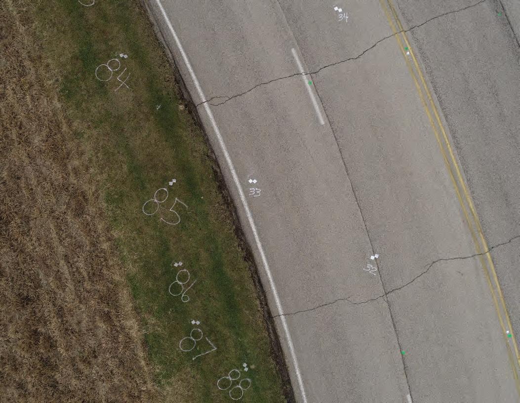
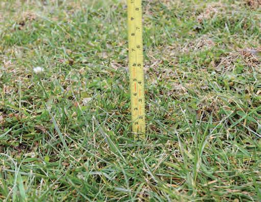
The testing took place at the Emergency Vehicle Operations Course (EVOC) of the Missouri State Highway Patrol, located in Jefferson City, Missouri. We selected four sites along the course, which provided varying degrees of grade and super-elevation. Additionally, the sites were composed of a variety of surfaces. After the sites were identified, a total of 100 test points were painted on the different surfaces at each site. Test points were painted using a template comprised of offset 0.3-foot squares, which touched only at one corner. White paint was used to paint most test points and all points were numbered. Figure 1: Test Points shows a sample of the test points painted on asphalt and grass.

Site one was exclusively asphalt. It was a large, banked curve with extreme super-elevation. The site was approximately 900 feet long. Site two was in an “S” shaped curve, had a change in grade, and incorporated a negative super-elevation. It was approximately 550 feet long. Of the 100 test points at site two, 64 were on asphalt and 36 were on grass. The grass was approximately 0.2-0.3 feet tall. Site three was mostly level and was approximately 450 feet long. There was a 0.35-foot curb on the asphalt that paralleled the roadway. At site three, 70 points were painted on asphalt and 30 points were painted on the varying height grass surface. The grass ranged from 0.2 feet tall to over 2.5 feet tall. Furrows were created in the taller grass using a string trimmer(weed-eater) and test points were painted on the ground in the furrows. Site four was approximately 700 feet long and consisted of both asphalt and gravel roadway. The asphalt road was

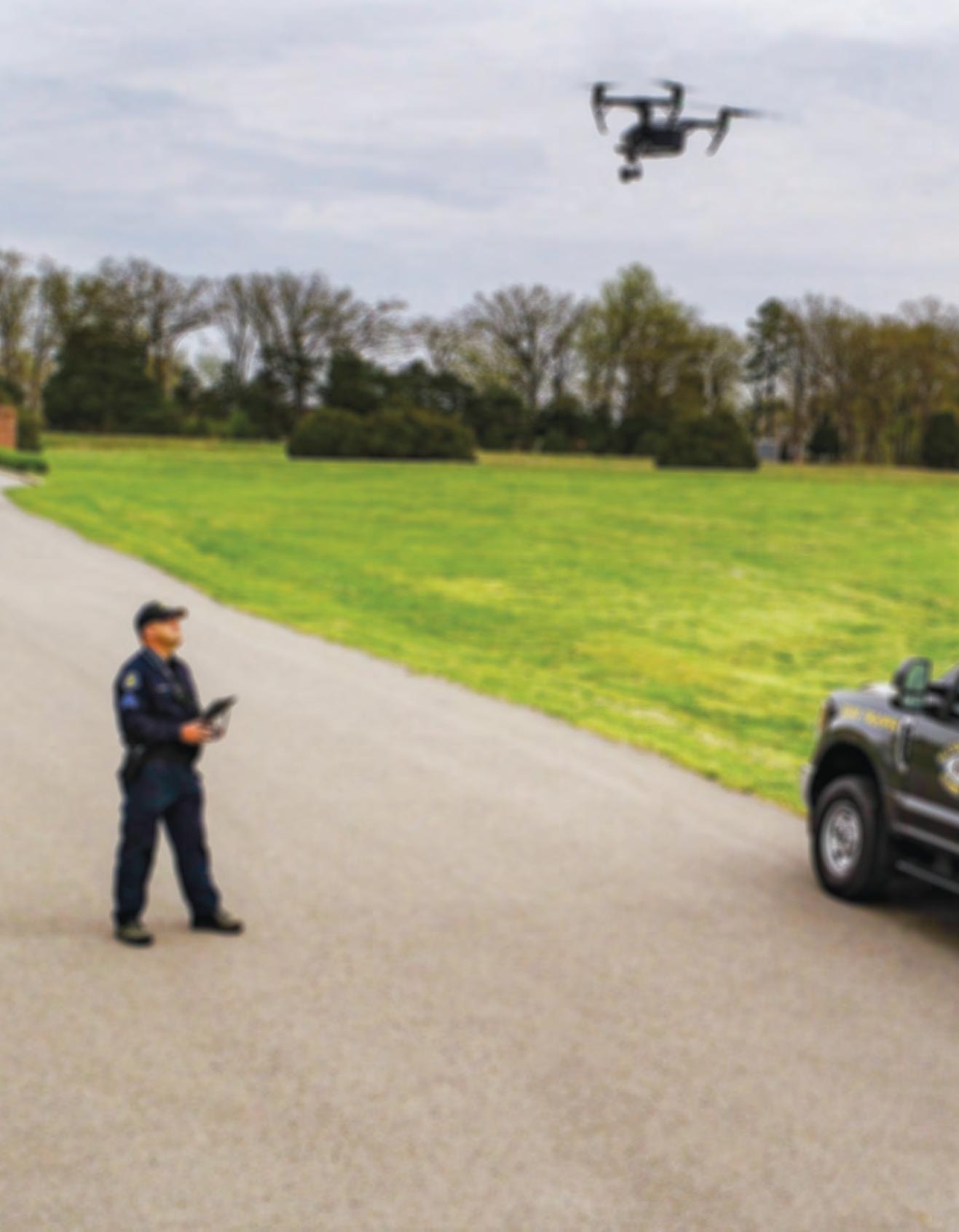
The sUAS used for this testing was a DJI Inspire 2 with a Zenmuse X4S camera. Each site was photographed in two separate ways. The first photographs were taken with the camera looking straight down at a 90-degree angle to the surface (ortho mode). The second group of photos were taken with the camera gimbal slightly angled (oblique mode). The oblique mode angle varied site to site but was between approximately 75 degrees and 90 degrees. This simulated flying a crash scene with moving traffic on the road without flying directly over the traffic. Existing federal regulations prohibit flying a sUAS above moving traffic.

For each mode used, the following guidelines were adopted. One pass was flown at approximately 100 feet above ground level (AGL). During this pass, photographs were taken with an overlap of approximately 80 percent. During this pass, each point along the test site should have shown up in mostly level. The gravel sloped down away from the asphalt. The gravel area was approximately the width of a one lane road. At site four, 80 test points were painted on the asphalt surface and 20 points were painted on the gravel. approximately five photographs. The second pass was flown at approximately 50 feet AGL. During this pass photographs were taken with an overlap of approximately 75 percent. This means each point should have shown up in approximately four photographs. During this pass if the entire width of the test area was not able to be seen, then two passes were flown at 50 feet and they overlapped in the center of the test area. The last pass was flown at approximately 25 feet AGL. During this pass there should have been 50 percent overlap of each photograph. This means each point should have shown up in approximately two photographs. Again, if the width of the test site cannot be seen in each photograph, then the photographs were overlapped near the center of the test site and two or more passes were flown. The only difference in the oblique passes was the sUAS was not flown over the “lanes of travel.”

In addition to the test points, ground control points (GCPs) were painted at each site. The ground control points were painted at each end of the test points and throughout the center. Site three, which had the “furrows” in the tall grass, had ground control points painted in the furrows and grass. Each site was mapped with a Sokkia iX robotic total station, using Magnet Field as the data collection software. To mitigate pole sway, the range pole was held by one person and the data collector was held by another. When the test points were documented, the total station averaged three shots to improve its accuracy. After the 100 test points were documented, the ground control points were documented. After documenting each site with the total station, it was flown and photographed with a sUAS.

After the test sites were documented with the total station and the sUAS, the photographs were loaded into PIX4D. PIX4D was the photogrammetry software used to process the scenes. Each site was processed separately with the ortho mode photographs and the oblique mode photographs. Each mode was developed with 5 or 6 ground control points and again with 10 or 12 ground control points.

Once the software finished processing the scene, the point clouds were turned off and test points were marked on the 3D mesh in PIX4D. The marked points were then exported in a comma separated value list. After this data was exported, each point was adjusted using the raw photographs in PIX4D. The data was again exported in a comma separated value list. Both lists were compared to the data collected with the total station.

The data was compared in the simplest form. The x,y,z coordinates documented with the total station, were compared to the x,y,z coordinates of each point documented with PIX4D. Then the straight-line difference was calculated between the two points. This distance was called the slope distance (SD). The following formula was used.

This yielded a real-world difference that was easily explained.

Results

When comparing the data sets, there was no appreciable difference identified between the orthogonal and oblique photography methods. There also appeared to be little difference between marking the test points only on the triangle mesh and using raw photographs to mark the location of each test point. The exception to this was in the grass and likely any other object that was not at ground level. When the test point was in the grass it had slightly less difference after it was marked on raw photographs. (This is also likely true for three dimensional objects like signs, vehicles, etc. but that was not tested).

Site One

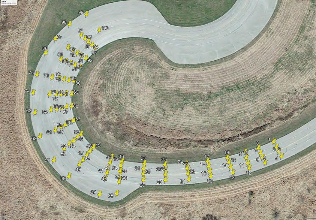
Site one was first processed with 5 ground control points. The location of the ground control points can be seen in Figure 4: Site 1-5 GCP X,Y. Notice the ground control points were placed in a colinear fashion. Site one is shown in Google Earth image Figure 2: Site one. The numbered push pins were also the location of the test points and correspond to the point number.

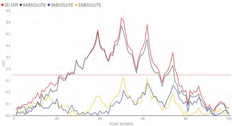
The data collected with the total station was compared to the data developed and documented in the 3D model using Pix4D. The results of that comparison are shown in the line graph Figure 3: Site 1-5 GCP. Looking at this data, the points near ground control points were more accurate. However, near the center of the curve, the difference grew to over 0.8 feet. When this site was initially processed, the PIX4D 3D model appeared accurate. There was no indication the test points near the center of the curve were off by nearly a foot.

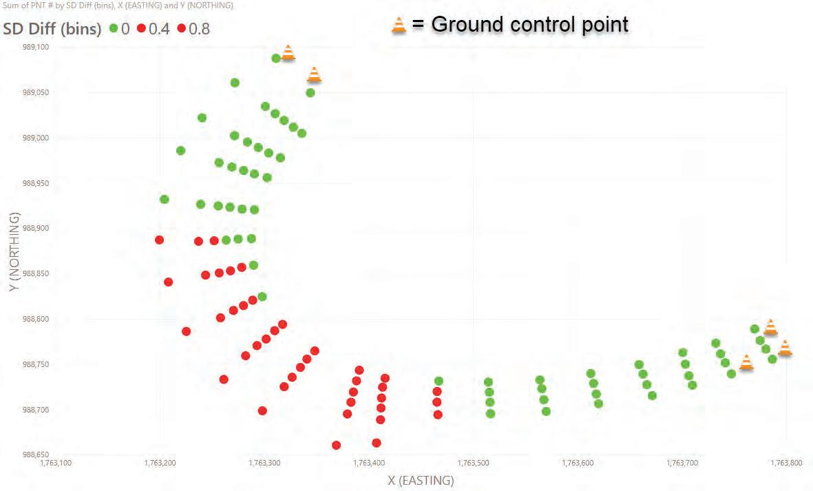
The data sets were also shown in a X,Y scatter chart with the test points plotted according to their X and Y coordinates (Figure 4: Site 1-5 GCP X,Y). Since the location of the test points was located with the total station in an X,Y,Z configuration it matched the shape of the test site. The test points in the scatter chart are color coded according to the length of the slope distance difference. The color code is shown at the top of the chart. This is useful because you can see how ground control points affected the accuracy of surrounding points.

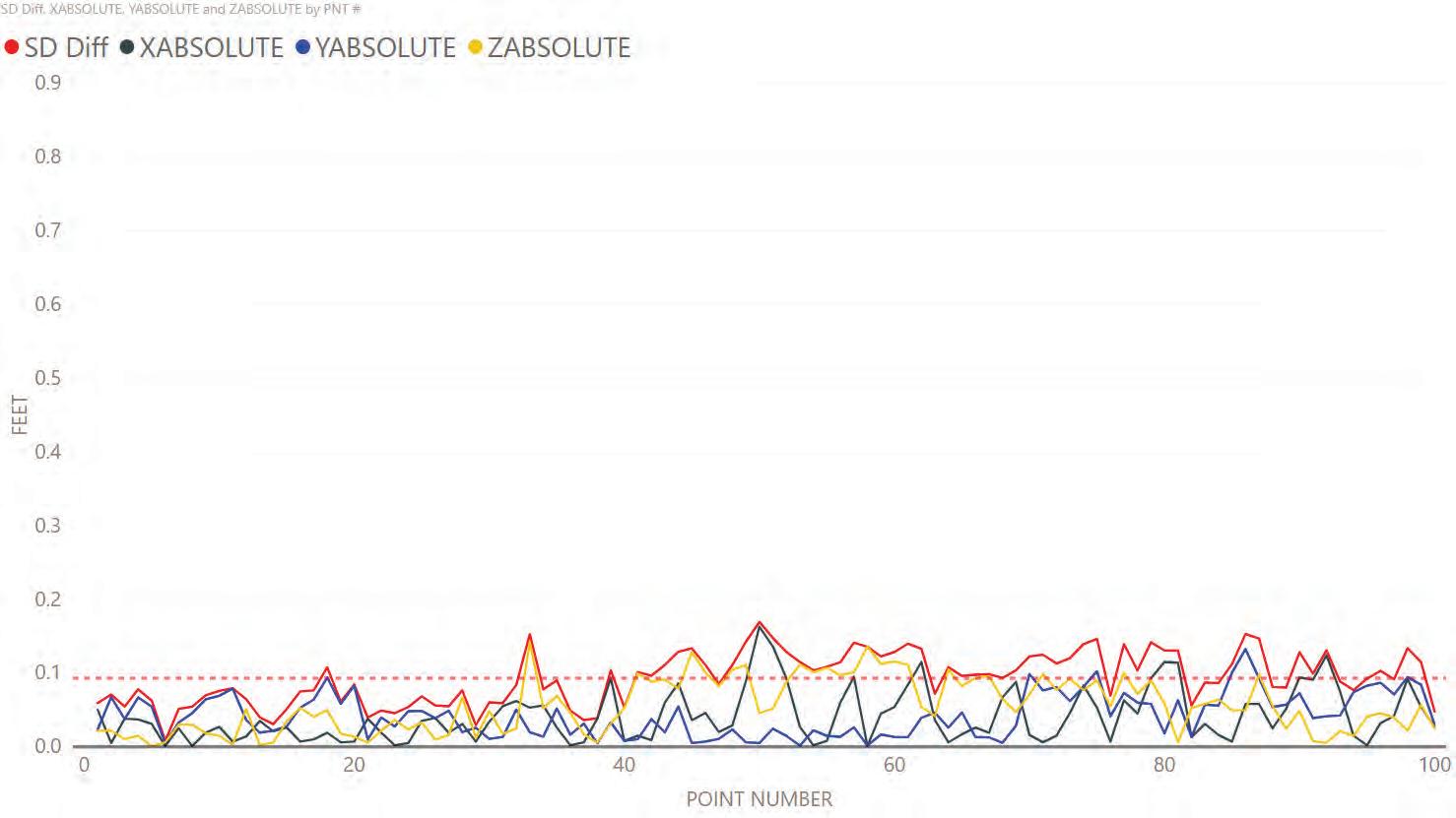
Site one was processed again with 10 ground control points. This time more widely spaced and non-colinear. The same method was used to compare the data. These results are shown in Figure 5: Site 1-10 GCP. The location of the ground control points can be seen in scatter chart Figure 6: Site 1-10 GCP X,Y.

The largest slope distance difference was less than 0.2 feet. The data was again plotted in a X,Y scatter chart with points color coded to indicate the slope distance difference. The color code is shown at the top of the chart. This was shown in chart Figure 6: Site 1-10 GCP X,Y.

The average final data for site one is shown in Table 1.

Site One

# of Photographs 2185 GCP10 GCP

Average 0.350.09

Minimum SD Difference0.040.01

Median SD Difference0.350.09

Largest SD Difference0.830.17

Table 1: Site 1 average final data

Site Two

Site two was comprised of points on asphalt and grass. It had gradual elevation and super-elevation changes. It was shown in Google Earth Image Figure 7: Site 2. The numbered push pins were also the location of the test points and corresponded to the test point number.

Site two data points one through 64 were painted on asphalt. Data points 65 through 100 were painted in the grass off the edge of the roadway. The height of the grass at site two was approximately 0.2-0.3 feet (as shown in Figure 8).

Site two was processed using 5 ground control points and again with 12 ground control points. The location of the ground control points can be seen in their respective scatter charts.

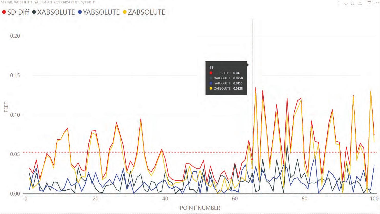
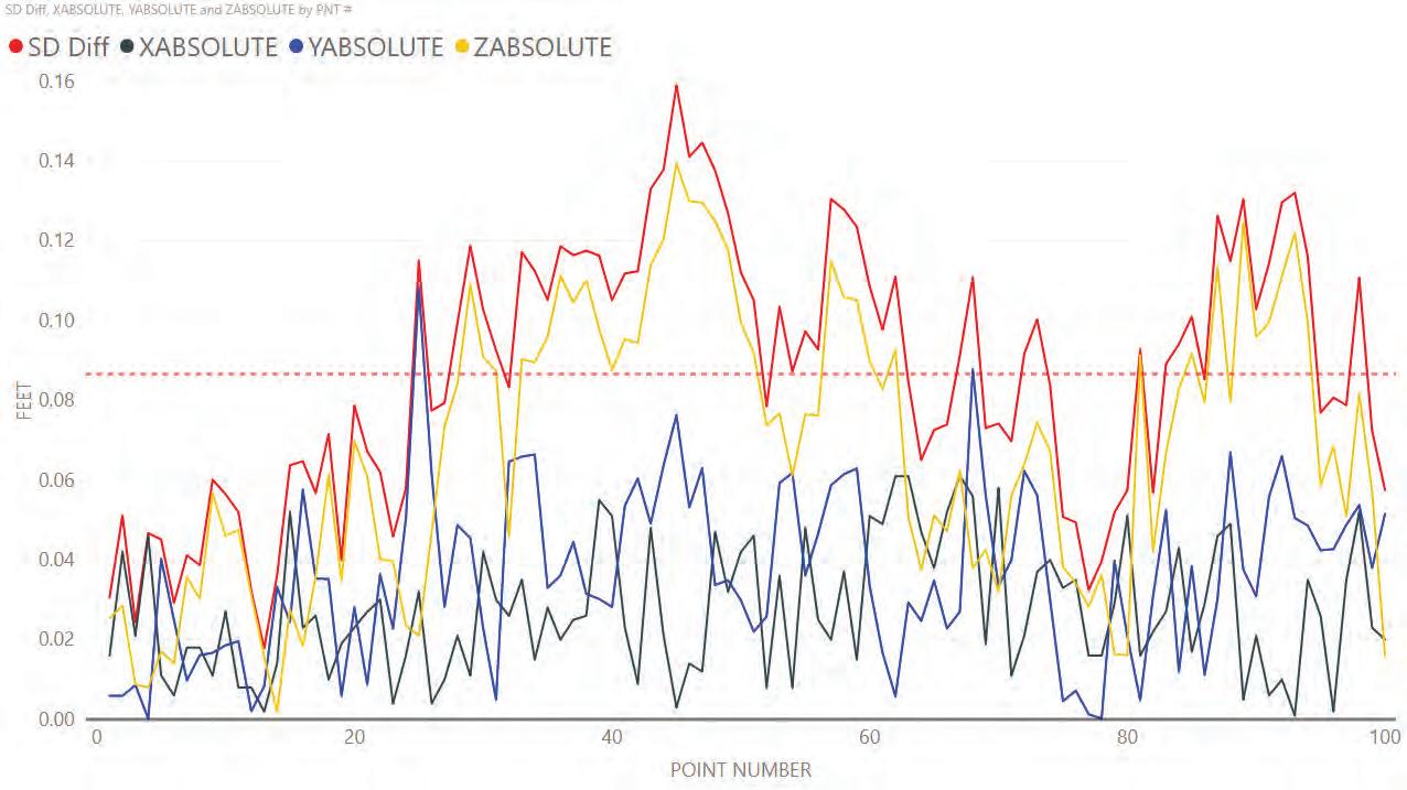
The data in Figure 9: Site 2-5 GCP shows the slope distance difference near point one and near point 63 (near the ground control points) is smaller. This illustrated the effectiveness of ground control points.

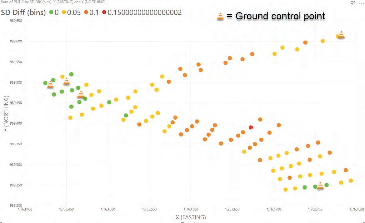
Figure 10: 2-5 GCP X,Y shows the test points plotted on an X,Y scatter chart. The same analysis performed in the site one scatter chart, was performed in this chart. The points were color coded according to the size of the slope distance difference. The color code is shown at the top of the chart. This graph helped illustrate the grass accounts for most of the error. However, there was a small section near the center of the test points that has a slightly larger difference when compared to each end of the site. It was here the ground control points were painted adjacent to the test points and not close enough to the super-elevation change to help build the model. Granted, the difference was small. Grass and soft soil present a few unique challenges when comparing total station data to the 3D model built using photogrammetry. The first problem involved the range pole and its tendency to sink into soft soil. That could not be accounted for using photogrammetry. The second issue we identified involved the depth and density of the grass. Photogrammetry cannot see into the grass to determine where the ground was or how deep the grass was. Therefore, what the photogrammetry software determined was the “surface” was influenced by the height of the grass and its density. Photogrammetry could only build a model to what it perceived was the “surface.” This was most likely the top of the grass. The third challenge was being able to consistently pick the exact same spot painted on grass with the range pole and in the photographs.

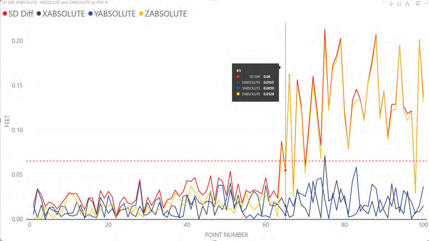
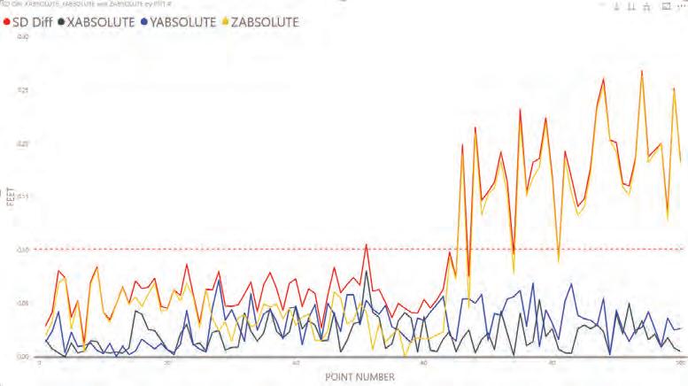
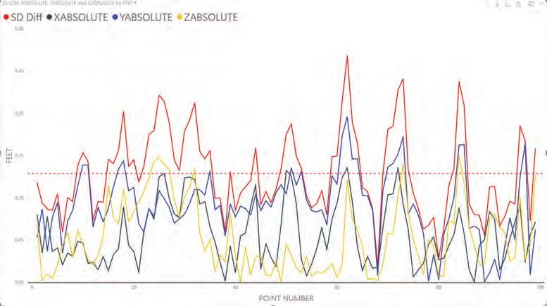
The data from site two with 12 ground control points is shown in Figure 11: Site 2-12 GCP. First, notice the scale was the same for both line graphs.

Like the data from site one, the average asphalt difference was lower on the model with 12 ground control points. This was because of the placement of ground control points near the center of the test site. However, notice the average difference in the grass, which starts at point 65 on both line graphs is larger.

The model with 12 ground control points had a larger slope distance difference in the grass when compared to the total station data than the model built with five ground control points. The larger difference is shown on the line graph. It appeared to be largely caused by the elevation difference. The slope distance difference almost mirrored the elevation difference. X and Y values remained very accurate.

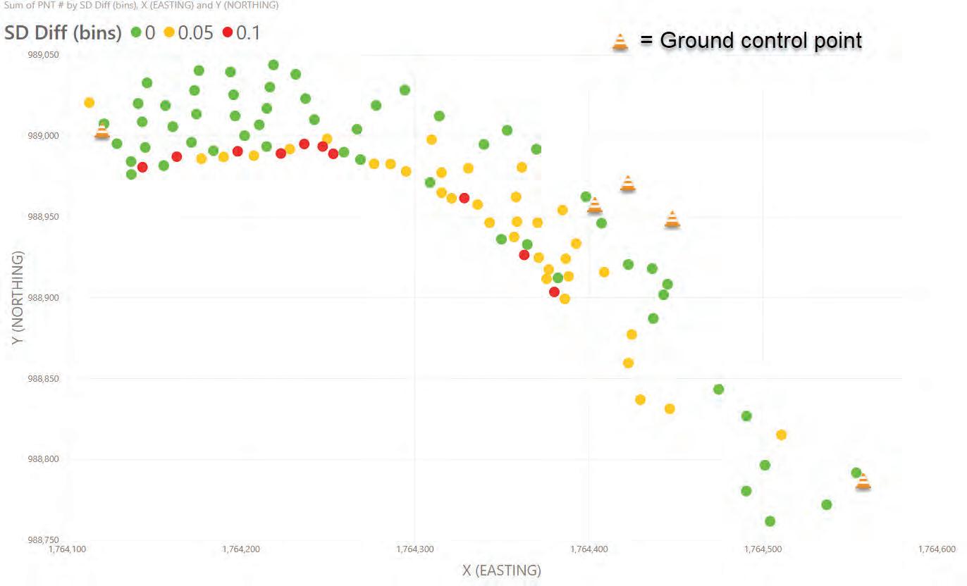
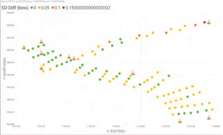
Notice when comparing the two “X,Y” scatter charts for site two, the area near the center no longer has the difference. The difference was negligible; however, ground control points made the model more accurate. The only area that had a slope distance consistently above 0.05 feet was grass.

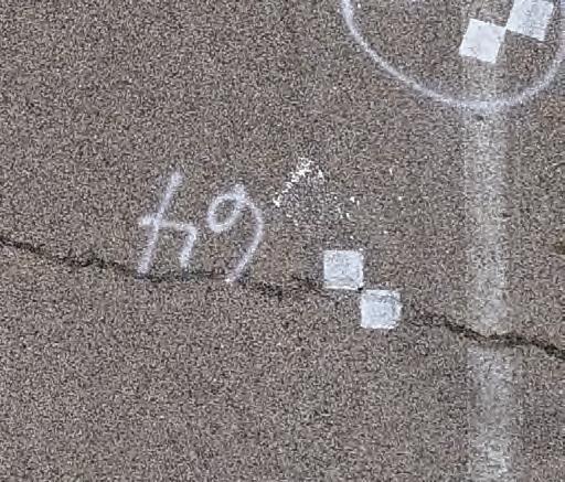
Another item worth noting, which highlighted the capabilities of photogrammetry, was found at point 64. In line graph Figure 11: Site 2-12 GCP, you can see point 64 was an asphalt point, yet its “Z” difference appears larger than the other asphalt points. While laying out the test site, point 64 fell on a crack in the asphalt. This is shown in Figure 13. While mapping this point with the total station the tip of the range pole went into the crack approximately 0.05 feet. The PIX4D software could not see this small hole in the asphalt and developed the triangle mesh at the surface of the asphalt. The larger slope distance difference for point 64 can be accounted for because the range pole went into this crack.

The data gathered from site two with 12 ground control points was shown in Table 2: Site 2 average final data.

Site 2

# of Photographs 421GrassAsphaltOverall

Average 0.130.030.07

Minimum SD Difference0.030.000.00

Median SD Difference0.130.030.03

Largest SD Difference0.210.090.21

Table 2: Site 2 average final data

Site Three

Site three lay in a relatively level area. The points numbered 1-70 were on the asphalt and the points numbered 71-100 were in the grass. Site three is shown in Google Earth im age Figure 14: Site 3. The numbered push pins were also the location of the test points and correspond to the point numbers.

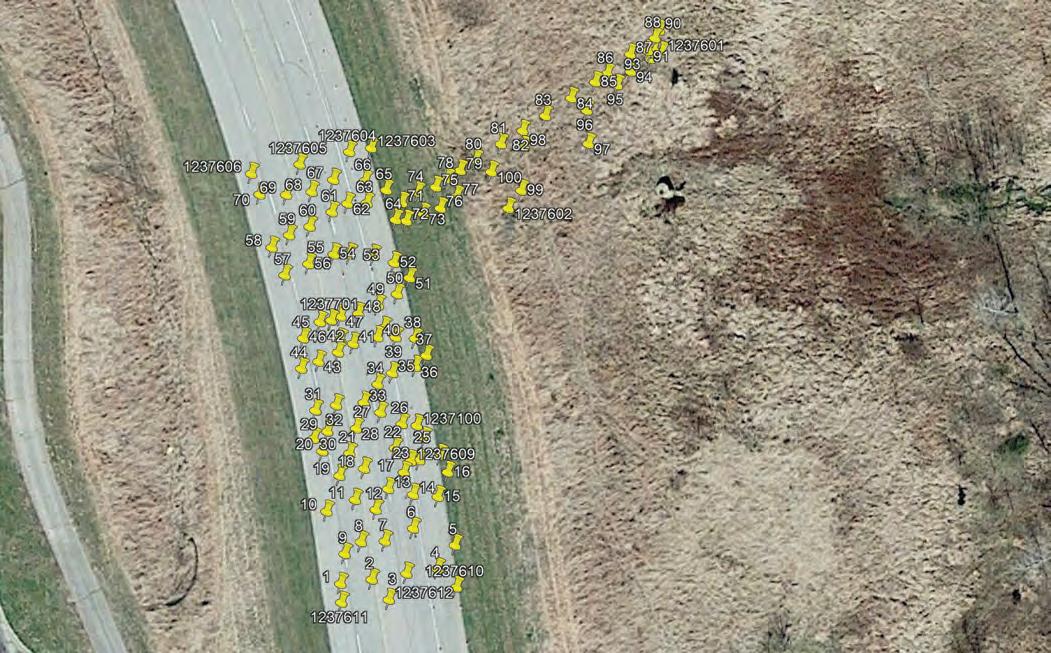
Approximately 12 feet from the east edge of the pavement there was a curb. The 12-foot shoulder was lower than the rest of the road. This curb was approximately 0.35 feet tall and was shown in Figure 15.

The grass ranged from 0.2 feet tall to approximately three feet tall. Grass taller than 0.2 feet had mock furrows cut into it with a string trimmer. The “furrows” were cut down to the soil. This did not replicate tires rolling across grass. Like the other scenes, the 3D model of this scene was first developed with five ground control points and then a second time with 12 ground control points.

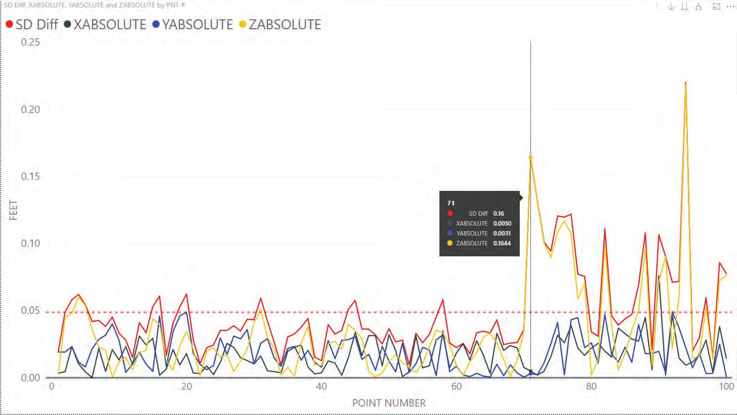
In the model built with five ground control points four of those points were painted on the asphalt and one was painted at the far-east end of the grassy area, on bare soil, in one of the simulated furrows. The location of the ground control points can be seen on the respective scatter charts. The scene was processed through PIX4D. Figure 16: Site 3-5 GCP shows the results of that data compared to the total station data. Note the scale of this graph is slightly different than the previous graphs.

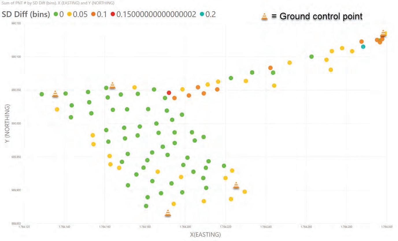
Examining the data revealed the slope distance difference on the asphalt surface was less than 0.1 feet. However, the points in the grass had a larger slope distance difference. That difference remained less than 0.25 feet. The points in the grass started at number 71. In Figure 17: Site 3-5 GCP X, Y, the test points were plotted on a X-Y chart. The points were color coded according to the difference in slope distance. The color code is shown at the top of the chart.

The data looked very similar to the data from site two. There was very little difference in the slope distance difference on the asphalt. The difference in the slope distance in the grass was mainly introduced by the elevation difference.

Site three was processed again with 12 ground control points. The results of that are shown in Figure 18: Site 3-12 GCP.

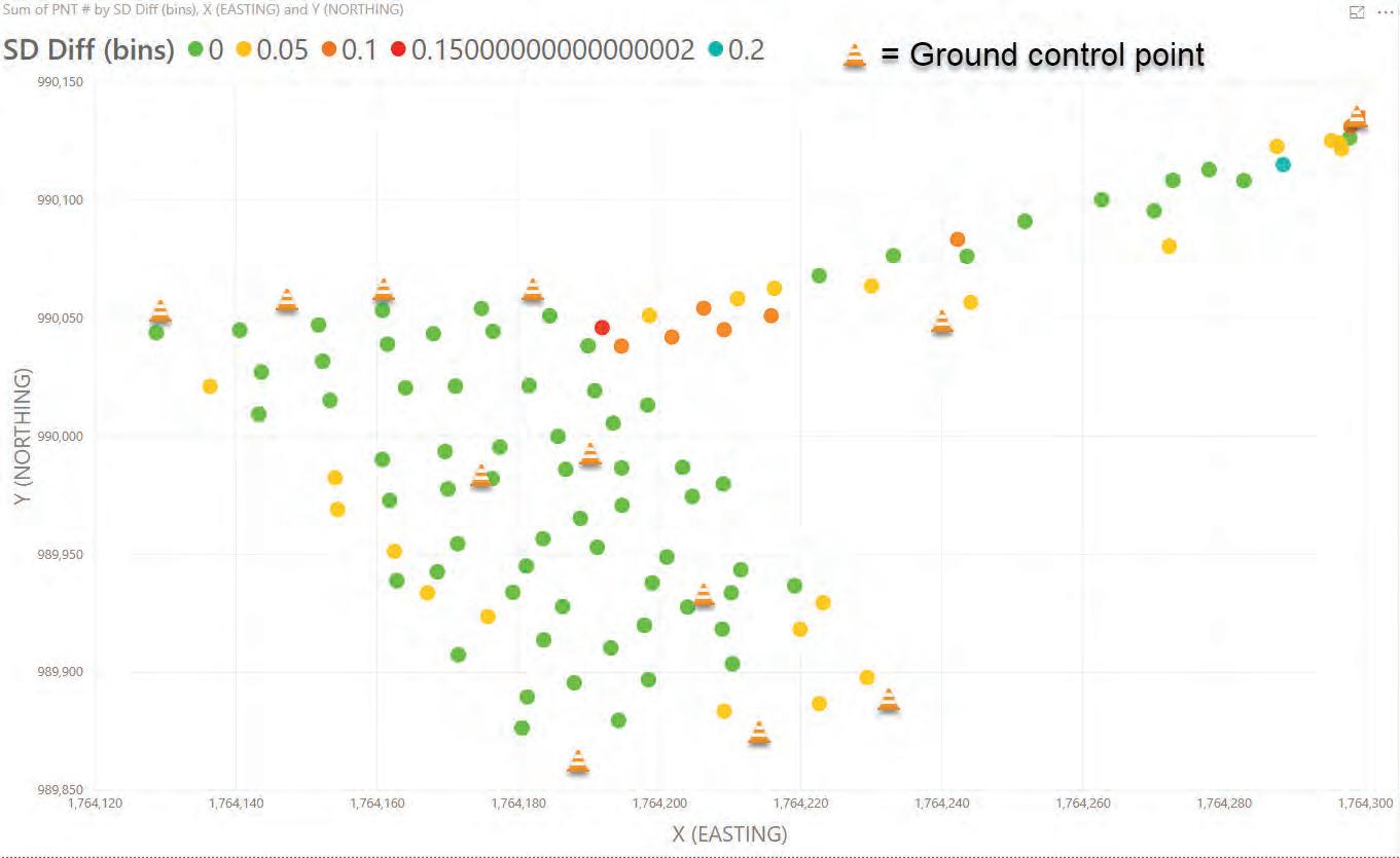
In Figure 19: Site 3-12 GCP X, Y, the points were plotted on an X-Y scatter chart color coded according to the difference in slope distance. The color code is shown at the top of the chart.

The additional ground control points on the asphalt slightly increased the accuracy. It was however, minimal. Looking at the data from the two 3D models generated by Pix4D there was not a significant difference. The data for site three with 12 ground control points is shown in table three.

Site 3

# of Photographs 261GrassAsphaltOverall Average 0.080.040.05

Minimum SD Difference0.010.010.01

Median SD Difference0.080.030.04

Largest SD Difference0.220.060.22

Table 3: Site 3 average final data

Site Four

Site four consisted of asphalt and gravel. The gravel was the approximate width of a one lane road. The asphalt was nearly level and the gravel road sloped down away from the asphalt. Site four can be seen in Google Earth image Figure 20: Site 4 The test points at site four started at the north end on the asphalt and continue toward the south on the asphalt to point 80. Point 81 was painted on the gravel at the edge of the asphalt and continued east to point 100. I used the data gathered using the “oblique” mode for this site. The 3D model was processed using five ground control points and a second time using ten ground control points.

A comparison of the data gathered with the total station and the 3D model developed using only five ground control points is shown in Figure 21: Site 4-5GCP. Ground control points were painted near point 1, point 80, and point 100. The location of the ground control points can be seen on the respective scatter charts. While the overall difference between the 3D model and the total station data was small, you can see ground control points appear to make the difference even smaller. Examining the line graph, it was evident the difference in slope distance was smallest near points 1, 80 and 100.

In Figure 22: Site 4-5 GCP X,Y, the points were plotted on an X-Y table and color coded according to the difference in slope distance when compared to the total station data. Again, the difference at each end of the asphalt near the GCPs is smaller. The color code is at the top of the chart.

The 3D model developed with 10 ground control points and compared to the data gathered with the total station is shown in Figure 23: Site 4-10 GCP.

This data showed the difference decreased slightly. This is negligible for most crash reconstruction applications. However, it illustrates the importance of ground control points. This can also be seen in Figure 24, Site 4-10 GCP X,Y. The points were plotted on an X-Y chart and color coded according to the difference in slope distance when compared to total station data. The color code is located at the top of the chart.

Site 4

# of Photographs 761GravelAsphaltOverall Average 0.080.060.06

Minimum SD Difference0.030.020.02

Median SD Difference0.070.060.06

Largest SD Difference0.150.090.15

Table 4: Site 4 average final data

Table 5 displays the overall averages for all sites. They were calculated using weighted averages for each surface. There may be slight differences because of rounding.

All site averages

GrassGravelAsphaltOverall Average0.1070.060.050.06

Table 5: All site average data

After the initial processing and comparison of the data, sites one and two were reprocessed using only the photographs taken at 100 feet AGL. Site one used 54 photographs and 10 ground control points. Site two used 38 photographs and 12 ground control points. The line graphs from those tests were shown in Figure 25: Site 1-100AGL and Figure 26: Site 2-100AGL. You can see the average slope distance difference increased for both 3D models. This could be because the 3D model was not as clear with only the 100- foot altitude photographs and was more difficult to mark. It was also a much smaller number of photographs.

The data from the model made with photographs taken at 100 feet AGL was compared to the data from the model using the “three-pass” method. When the “three-pass” method was used it increased the accuracy slightly and produced a much more detailed 3D model.

Conclusions

Employing the methods described above, the use of small unmanned aircraft systems, in conjunction with modern photogrammetry software, is a cost-effective option for documenting crash scenes. However, the placement of ground control points is paramount to the development of an accurate 3D model. Through this testing, it was discovered ground control points shouldbe placed in a non-colinear fashion and widely dispersed throughout the scene. If increased accuracy is desired these six locations should be considered:

• Each end of the scene

• Near the center of the crash scene

• At significant elevation changes critical to the crash investigation

• Along significant curves

• Near areas of crucial evidence

• When evidence is in the grass, in furrows or large gouges

Using the data from site one it was discovered without a way to check the 3D model it could be inaccurate in some areas. To combat this, we placed “check points” in a few areas between ground control points. The location of these “check points” was recorded, but not used to build the 3D model like a ground control point. After the model was built, the location previously recorded was compared to the location of the “check point” in the 3D model. This method worked well for validating the 3D model.

The data demonstrated the proximity to ground control points increased the accuracy of points within the 3D model. Of note regarding the testing was the problem posed by grass. The tests conducted involved grass, that ranged from approximately 0.2 feet to approximately three feet. Grass taller than approximately 0.2 feet was trimmed to the soil to simulate furrows. The surrounding grass was not trimmed or laid down. When processing a 3D model with tall grass it must be understood it will most likely have larger errors than demonstrated here unless the soil is visible and ground control points can be placed on the soil directly. The photography and modeling process used in this testing was in accordance with the training received by the Missouri State Highway Patrol Major Crash Investigation Unit. I have not used any other method or attempted to validate any other method of photogrammetry.

About the author: Master Sergeant Joseph Weadon, III is a 22-year veteran of the Missouri State Highway Patrol. He is currently assigned to the Major Crash Investigation Unit and is the Team Leader of Team #4.

Acknowledgements: Aerial Metrics, Stan Taylor and Iain Lopata. Sergeants Paul Meyers, and Glen Ward; and Trooper Dan Yingling.