Mark your calendar!

March 9-11, 2020 - Houston, Texas www.crashdatagroup.com/edr-summit

The EDR Summit will deliver the next steps in advanced EDR technology for vehicle crash analysis. Most importantly, this summit brings together industry experts from around the world to present on timely topics and case studies.

The presentations will focus on EDR data found in light trucks, passenger cars, SUVs, motorcycles, heavy commercial vehicles, active safety systems, autonomous driving, and vehicle infotainment systems.

The EDR Summit is open anyone who has an interest in learning more about event data recorders and how they are used in vehicle safety and crash investigation. As a result, typical attendees of this Summit include law enforcement, insurance (SIU and claims), government, legal and collision reconstructionists. Therefore, if you are involved with the collection and/or analysis of EDR data from vehicle crashes or forensics you won’t want to miss the EDR Summit!

Extant closed-form analytic solutions for quantifying residual damage based model parameters, equivalent barrier speed (EBS) and internal work absorbed (IWA) that use the residual damage profile present after a collision are predicated upon the employment of global or piecewise linear interpolation at the level of the residual damage profile. The subject work focuses, primarily, on the theoretical evaluation of this predicate. This evaluation is approached first by defining the residual damage depth function as the difference between the reference and damaged boundary geometry functions. It is shown that the extant formulation is reproducible when both boundary geometry functions are separately linear (interpolated or otherwise) over a mutual domain. It is also shown that the presence of non-linearity in either boundary geometry function also appears in the residual damage depth function and thereby changes the form of the equations that are currently employed for determining the relevant parameters. The case in which the interpolation function for the reference boundary geometry consists of a general polynomial function is detailed in depth. A worked example is provided in which other forms of interpolation functions are considered for both the reference and damaged boundary geometries.

Introduction

Equations (1-2) are the most commonly employed mathematical relationships that serve as foundational for the determination of collision severity as a function of the residual damage present to a motor vehicle following involvement in an impact (Sharma et al., 2007). The first of these equations, proposed by Campbell (1972, 1974), is an empirical relationship between the depth of residual damage (c) and the equivalent barrier speed (EBS). The second equation, proposed by McHenry (1976), relates the residual damage depth to the peak collision force magnitude, |F|, normalized to the reference configuration direct damage contact width (L) and is one of the critical relationships in the third iteration of the Calspan Reconstruction of Accident Speeds on the Highway (CRASH3) damage analysis algorithm. This relationship is analytic for the closure phase of a coaxial collision when the structural response characteristics of the collision partners are modeled as linear elastic (Noga and Oppenheim, 1983) but becomes empirical in consider- ation of collisions with a separation phase for which the coefficient of restitution is not zero-valued.

The internal work absorbed (IWA) during a collision can be directly related to the EBS and the mass of the collision partner (m) as shown by equation (3).

The relationship shown by equation (2) is not a timeparametric force-deflection response nor does it represent a time-parametric force-deflection response shifted along the abscissa. The force-deflection data generated from any singular collision test, for example, maps to a single point along the response curve. In practice, however, this relationship is treated as being equivalent to a time-parametric force-deflection response in regards to the determination of the IWA.

Traditional solution for IWA for uneven damage profiles

In the consideration of residual damage profiles for which the depth of residual damage varies as a function of location along the width of the direct damage portion of the profile, the traditional approach has been that of using a discretization scheme consisting of the piecewise employment of the trapezoidal rule using two, four or six equally spaced nodal points. This was extended to the use of any N number of equally spaced nodal points (Singh et al., 2003) and then for the use of any N number of unequally spaced nodal points (Singh, 2005a). The latter presentation, being the most general, is considered herein. In this regard, the independent variable, l {l: 0 ≤ l ≤ L}, denoting the location along the width of the direct damage portion of the residual damage profile, in the plan view and mapped to the reference configuration, is introduced. The residual damage depth function may then be stated as c(l). The ith {i: 1 ≤ i ≤ N} nodal value of the residual damage depth, located at li, is denoted as ci. The linear interpolation function between successive nodal values derives from the simple definition of a two-dimensional line.

Following the traditional approach to determining the IWA, equation (2) is integrated over the residual damage domain.

Traditional solutions for the model coefficients

Substitution of equation (4) into equation (5) followed by evaluation of the final integral yields the following result:

The traditional solution for the model parameters proceeds by equating the IWA based on equation (3), following substitution for the EBS from equation (1), to the solution for the IWA from equation (8). Both equations are second order polynomial equations with respect to the residual damage depth and are only equal when the coefficients, from each equation, for each order of the polynomial, are equal. This approach allows for the development of the following relationship between the coefficients of the two models.

Unlike a time-parametric force-deflection relationship, the ordinate intercept of the response function, shown by equation (2), does not fall at the origin. A consequence of this result is that the abscissa intercept occurs at a value of c o=-AB-1. The area bounded to the left of the ordinate, above the abscissa and below the response curve can be determined by integration.

Substitution of these equivalencies into equation (8), followed by algebraic rearrangement, results in the following quadratic form for the Campbell b1 model coefficient.

(7)

The traditional solution for the IWA for each zone (i.e. the region between successive nodal points) is obtained by adding equations (6) and (7). Summation of the result over all zones from i = 1 to i = N-1 yields the IWA for the entire residual damage profile. AB IWA GL 26 =α+β+ (8) Where:

In practice, the Campbell b0 model coefficient, representing the maximum EBS at which no residual damage depth is produced, is estimated and the IWA is written in terms of the EBS.

The positive valued solution for equation (13) fits the physical nature of the modeling problem under consideration.

The traditional approach when considering a collision force vector that acts at an angle θ, with respect to the relevant vehicle principle axis, is to employ trigonometric relationships such that the force considered is F sec(θ) and the residual damage is c sec(θ). The resultant form of equation (8), as a result, contains the multiplicative term sec2(θ), which is equal to 1 + tan2(θ).

When θ is not zero-valued, this solution becomes:

Back-substitution of equation (15) into the three relationships listed under equation (11) allows for the determination of the CRASH3 model coefficients. This approach is typically employed in the case in which one seeks to quantify the model parameters, on a vehicle platform-specific basis, from controlled collision testing in which the testing configuration consists of a colinear full-width engagement impact between a test vehicle and a fixed, rigid, massive barrier (FRMB). For testing in which both collision partners are deformable (Neptune et al., 1992; Neptune and Flynn, 1998; Singh, 2005b) or for field studies for which the model coefficients of only one collision partner are known (Hull and Newton, 1993; Neptune and Flynn, 1994; Long, 1999; Chen et al., 2005), the solution procedure is based on implementing Newton’s Third Law, with the procedure referenced in the previous literature as the force balance method. Using the subscript A to denote the collision partner for which the model coefficients are known, the zonal force is expressed as:

The structural response approaches detailed above and considered herein are uniaxial compressive. The models do not contain an explicit mechanism for the inclusion of deformation and residual damage due to transverse shear or out of plane bending. In theory, the uniaxial compressive response can be taken with respect to an arbitrary, inplane, orientation with respect to the principle axes of a vehicle when considered with respect to the plan projection (i.e. with respect to the plane based upon the longitudinal and lateral axes). In practice, however, the vast majority of controlled collision test data is reported with the residual damage depth information taken along the relevant principle axis and with respect to the reference configuration. While this is a limitation, it does provide for simplifications in regards to the focus of the subject work, which is detailed as follows.

Objectives

The zonal force equation for the opposing collision partner, referenced using the subscript B, can be expressed as:

When the model coefficients are constant across all of the zones of direct damage, the zonal indication associated with the model coefficients in equation (17) can be dropped. The total force is obtained by summing equation (17) over all zones.

The value of the collision force, in equation (18), however, must be equal to the value of collision force obtained by summing equation (16) over all zones of direct damage. Substitution from the relationships under equation (11) into equation (18) followed by algebraic rearrangement results in the following quadratic equation:

The residual damage present to a vehicle, following a collision, clearly represents the difference between the reference geometry of a vehicle and the deformed (i.e. damaged) geometry of the same. Equations (1-2) are clearly linear functions of the residual damage depth and the subsequent derived quantities are clearly predicated upon this linear presumption. The extant literature includes a number of alternative linear static models such as the constant force model, the saturation force model, the bilinear stiffness model (Strother et al., 1986; Kerkhoff et al., 1993) and the multilinear stiffness model (Singh and Perry, 2008) as well as the nonlinear static power law model (Nilsson-Ehle et al., 1982; Woolley, 2001; Singh and Perry, 2008). One area that has not been explored, however, and represents the objective of the subject work, is the evaluation of the relationship between the reference and deformed geometries and the assumption of linearity in regards to their difference, defining the residual damage profile, and the derived quantities that are based upon the difference.

Theory

Axes mapping and generalized coordinates

The solution for the Campbell b1 model coefficient is again the positive valued solution for the quadratic and with the A, B and G model coefficients determined by back-substitution.

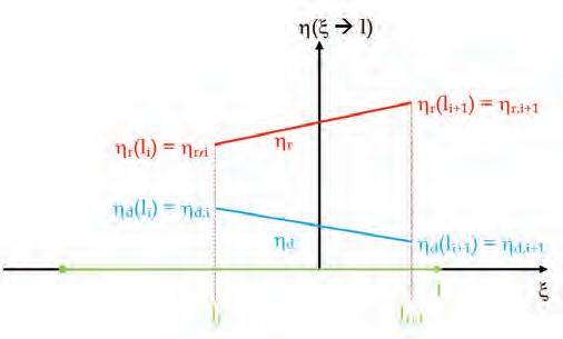
For the plan-projected view the relevant vehicle principle axes are the longitudinal axis (x) and the lateral axis (y). The mathematical expressions for the front and rear aspects of the geometry boundary models may be expressed as x = f(y) whereas the left and right sides of the geometry boundary models may be expressed as y = f(x). Both cases can be expressed in a singular compact form by denoting the independent variable as ξ (where ξ = y for the end case and ξ = x for the side case) and the dependent variable as η = f(ξ). There are two important consequences that arise from the assumed uniaxial compressive structural response model. The first is that the vehicle axes in the reference and deformed configurations remain coincident. The second is that the mapping of l ↔ ξ and c(l) ↔η(ξ) can readily be related to the reference configuration. Denoting the reference boundary geometry as ηr(ξ) and the deformed boundary geometry as ηd(ξ), the residual damage depth function can readily be written as:

Linear boundary geometr y functions

The simplest plan-view boundary geometry model is that of the rectangular approximated boundary geometry model for the reference geometry. This model is parameterized by the maximum overall width and length of a vehicle and is geometrically represented by a rectangle. Any boundary region of the model is therefore defined by a zero-valued slope with respect to the relevant principle axis. One may readily consider the more general form of this model (i.e. for non zero-valued slopes). Using the axis mapping discussed above, for the case in which both the reference and damaged geometry boundaries are linear functions over a mutual domain {l: li ≤ l ≤ li+1}, the equations for the segments are:

The nodal values of the residual damage depths are:

Substitution of these definitions from equation (24) into equation (23) results in the following:

As expected, equation (25) exactly matches equation (4). It therefore follows, again, as expected, that the case of the linearly modeled boundary geometry functions for both the reference and damaged geometries, over a mutual domain, produce the linear interpolation function for l-c(l) that is employed in the extant formulation. This will clearly have a direct impact on the IWA formulations for which c(l) is a limit of integration. It can also be shown that the form of c(l) impacts the relationship between collision force and the depth of residual damage.

The boundary geometry functions are shown schematically in Figure 1.

Substitution of equation (25), which again derives from the case in which both the reference and damaged boundary geometries are linear functions over the mutual domain, into equation (26) followed by evaluation of the integral results in the following solution.

Non-linear boundar y geometry functions

Figure 1: Reference and damaged linear boundary geometry functions over a mutual domain.

Substitution of the two equations under (22) into equation (21) results in the following solution for the residual damage depth function:

The number of potential forms and formulations for alternative functions for modeling the boundary geometries is legion and the exploration of all such cases is beyond the scope of this work. The argument, however, can be made that nonlinearity in either boundary geometry function, that is not removed by the subtraction operation of equation (21), becomes manifest in the residual damage function and therefore in the collision force and IWA relationships. If ηr(l) = f(λr1, λr2) and ηd(l) = f(λd1, λd2) where λr1 and λd1 are linear terms and λr2 and λd2 are nonlinear terms then the following holds:

The functional dependencies shown for c(l), in the relationships shown under equation (28), hold to the extent that λr1 ≠ λd1 and λd1 ≠ λd2. The presence of the same category of terms (i.e. linear or nonlinear) in both boundary geometry models would generally be expected to result in the same category of terms appearing in the difference given that the points used to generate each boundary geometry model are not mutually inclusive. The theoretical development for one family of functions is considered below.

The linear functions considered thus far are simply first order polynomial expressions. A simple approach, first, for consideration of the impact of nonlinearity, is by increasing the order of the polynomial function used to model one of the boundary geometries by a single order. Either one or both of the boundary geometry functions may be modeled in this way. For this presentation, the damaged boundary geometry function is left unchanged and the resulting functions over the mutual domain may be written as: relationship between the collision force and the depth of residual damage becomes:

Equation (31), either for a single zone of direct damage or for the entire width of direct damage, would result in a differing quantified value not only for the total collision force magnitude, but also for the downstream quantified model coefficients for the cases when the force balance approach is employed. For the sake of comparison, rewriting equation (25) in an equivalent first order polynomial form and rewriting equation (27) leads to the following form:

The zonal form of equation (10), for the IWA, for the first order polynomial for c(l), can be rewritten as:

In equation (29), the terms associated with l and l2 are presented without an offset term (i.e. in the form of l – li). For the case in which a polynomial is used, the function becomes interpolating rather than approximating when the number of nodal points used in generating the polynomial is one greater than the order of the polynomial. Therefore, the functional domain of the second equation under (29) can fully be defined by the nodal points located at l = li and l = li+1, whereas the functional domain for the first equation, in the interpolation sense, would have the two nodal points within its domain. The residual damage function is obtained as before.

For the second order polynomial form for c(l), the zonal IWA becomes:

The polynomial coefficients in equation (30) encode the nodal values for both the reference and damaged boundary geometries as well as the residual damage depths, which can be retrieved by solving c(l) at l = li and at l = li+1. The

The use of polynomial functions of arbitrary order further supports the view that uncancelled nonlinearity in the difference between the reference and damaged geometries becomes manifest in the residual damage function and the terms that derive from it. If the order of the polynomial function for the reference boundary geometry is denoted as p and that of the damaged boundary geometry is denoted as q then the maximum polynomial order under consideration is n = Max(p, q). Both boundary geometry functions can be expanded to this maximum order by setting the coefficient terms associated with each order beyond the normative order equal to zero. The boundary geometry functions may then be written as:

The residual damage function may then be written as:

There does not appear to be a simple method for expressing the integral in equation (42) in an evaluated form as it relates to the product operator in the integrand. The zonal IWA, for this case, is:

The peak collision force magnitude, in closed form, for this case, becomes:

Worked Example

A closed form solution for the IWA, for this case is only partially determinable. The term associated with the A coefficient is:

The solution for the term associated with the B coefficient proceeds by employment of the multinomial theorem, which can be written

The term to the right of the equality in equation (39) can alternatively be expressed as:

In equation (40), the kt terms are the coefficients associated with the terms in the polynomial expansion. For example, for a third order polynomial raised to the second power, the expansion would consist of six terms, each of which would involve k1, k2 and k3 being set to zero, or two with the sum of the k t values for each term being equal to two. For the subject case:

The term associated with the B model coefficient is only partially reducible, in a closed form sense, for this case, as:

The Vehicle Crash Test Database (VCTB) of the National Highway Traffic Safety Administration (NHTSA) was queried in a semi-random manner for a Federal Motor Vehicle Safety Standard (FMVSS) 208 or high-speed frontal New Car Assessment Program (NCAP) test conducted for vehicles falling within the last decade of model years. Test No. v08781 (NCAP test for a 2015 Hyundai Genesis four door all wheel drive sedan) was selected from the resulting set of tests. The as-tested vehicle mass (2192.5 kg) and test vehicle speed at the start of closure (56.3 KPH) were taken directly from the contractor’s report for the collision test. Residual damage profile information for collision testing of this type follows one of two formats. The first is reporting the distance aft from the reference centerline location. The second is reporting the distance from a datum reference at the rear surface of the vehicle. In regards to the second method, it is assumed that the datum reference plane is tangent to the rear surface of the vehicle at the centerline. The second method was used in regards to the reporting of the longitudinal dimensional data at the damage profile distance six (DPD6) locations. This dimensional data was converted into x-axis coordinate data by subtracting the reference configuration values for the rear overhang (Expert AutoStats v.5.5.1; 4N6XPRT Systems; La Mesa, California), the reported wheelbase and adding the reported longitudinal distance of the as-tested center of mass aft of the front wheels center. The y-axis coordinate data for the same six points was determined by noting that the location of the direct damage width midpoint was at the centerline of the test vehicle in its reference configuration and that the spacing between consecutive nodal locations was at a distance of 0.2 L (L = 1.520 m). A seventh point, that which was located at the reference centerline of the test vehicle, was also considered for inclusion. The inclusion of this point, however, proved problematic in that the resultant plan-view projected boundary geometry of the front of the test vehicle was pointed, in an exaggerated manner, at the centerline, and inconsistently so with respect to the observable frontal geometry boundary shape as per qualitative examination of the pre-test photographs. As a consequence, only the DPD6 locations were considered for both the reference and damaged boundary geometry modeling tasks. The reference coordinate data points, in units of meters, were determined to be (-0.760, 2.162), (-0.456, 2.273), (-0.152, 2.315) and with symmetry about the test vehicle centerline, in the reference configuration, for the remaining three data points. The damaged coordinate data points, in units of meters, were determined to be (-0.760, 1.833), (-0.456, 1.831), (-0.152, 1.858), (0.152, 1.806), (0.456, 1.814) and (0.760, 1.801).

The following tasks were undertaken (all evaluations were conducted using Mathematica v.11.2; Wolfram Corporation; Champaign, Illinois):

1. Comparing the extant methodology, as per equation (14), for which the use of piecewise linear interpolation is employed for the residual damage function, against the formulation, based on the use of equations (21) and (22), which employs piecewise linear interpolation at the level of the reference and damaged boundary geometries. Showing an equivalency of the b1 model coefficient is sufficient for showing equivalency for the A and B model coefficients when the damage onset EBS (b0), the width of direct damage (L) and the mass of the vehicle (m) are held constant.

2. Comparing the results of the extant methodology against that based on the employment of the use of simple polynomial interpolation for both the reference and damaged geometries.

3. Comparing the results of the extant methodology against the results based upon the use of other interpolation methodologies (spline interpolation and Hermite interpolation).

For the first task, the use of the as-reported nodal residual damage depths resulted in α = 1.3449 m2 and β = 9.01624∙10-1 m3. The solution for the b1 model coefficient, for both the extant method and the use of piecewise linear interpolation at the level of the reference and damaged boundary geometries resulted in the following solution (with b0 expressed in units of m/sec and b1 expressed in units of sec-1):

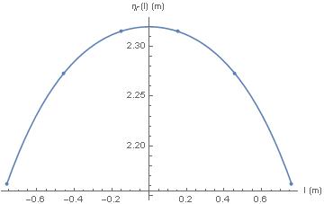
The resultant reference boundary geometry model for this case is shown in Figure 2.

The use of polynomial interpolation for the reference data resulted in the generation of an exact fit (adjusted R2 = 1), using a fourth order polynomial function, and with no exhibition of Runge’s phenomenon. The interpolation equation was:

Figure 2: Reference boundary data points and the resultant fourth order polynomial interpolation fit through the data. Note that the origin shown is not at a zero-value along the ordinate

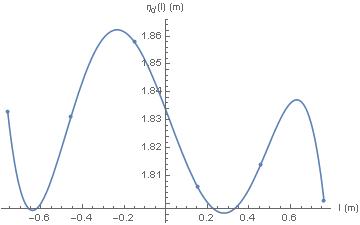
Fitting of the damaged boundary data points with a singular polynomial function proved to be highly problematic. The adjusted R2 values for fits from the first through fourth order were, 0.301698, 0.221018, 4.53928∙10-3 , and -0.932776, respectively. The fifth order polynomial interpolation, through this data, exhibited the undulations between the data points that are characteristic of Runge’s phenomenon. This is shown in Figure 3.

Figure 3: Data points for the damaged boundary geometry and the fifth order polynomial interpolation function for fitting the data

Polynomial interpolation for the second task, due to the problematic nature of the fit, was not used. Instead, for the second task, the damaged boundary geometry was modeled in a piecewise linear manner while the fourth order polynomial function shown by equation (45) was used for the reference boundary geometry model. The residual damage function that was generated consisted of five piecewise fourth order polynomial functions. The resultant solution for the b1 model coefficient is:

For the case of spline and Hermite interpolation, the inbuilt Interpolation function was used for both the reference and damaged boundary geometries. The interpolation method was specified within the function call as was the interpolation order. Visual inspection of the resultant, for the spline function, revealed no significant change in the visual appearance of the resultant beyond an interpolation order of two for both the reference and boundary geometries. A similar approach for the Hermite interpolation function revealed an interpolation order of three for the reference boundary geometry and two for the damaged boundary geometry. In the latter case, a higher order interpolation resulted in the exhibition of Runge’s phenomenon. The residual damage function was then determined for each pairwise case for the reference (piecewise linear, polynomial, spline and Hermitian) and damaged (piecewise linear, spline and Hermitian) boundary geometry models. The use of the inbuilt interpolation function resulted in the generation of Interpolation Objects for c(l). The Interpolation Objects for both c(l) and (c(l))2 were numerically integrated and with the numerical results serving as a portion of the coefficient values in the quadratic form of the Campbell b1 model coefficient equation. That being:

Figure 4: Residual damage functions based upon the use of piecewise linear (left), spline(center) and Hermite (right) modeling of the damaged boundary geometry. For each plot, piecewise linear (blue), polynomial (red), spline (green) and Hermite (orange) models were used for the reference boundary geometry

Table 1: Constant terms for the form of the Campbell b1 model coefficient based upon the form of equation (48) and as a function of the type of boundary geometry models used for the reference and damaged boundary geometries

The form of equations (44) and (46) serve as examples of a convenient generalized form for expressing the solutions for the Campbell b1 model coefficient. This form is given by equation (48), in which the terms a1 through a4 are constants that are expected to differ based upon the forms of the reference and damaged boundary geometry models that are used to generate the residual damage function. 2 1102340 b abaaab

The residual damage functions are shown in Figure 4 and the constant coefficients are shown in Table 1.

The response shown by equation (48) is that of a linear response of the Campbell b1 model coefficient in regards to the Campbell b0 model coefficient. This linear response was shown by plotting each function, as shown in Figure 5, over a reasonable domain of b0 values.

For a nominal b0 value of 1.1176 m/sec (2.5 MPH), the minimum b1 value was 32.2930 sec-1 (polynomial reference boundary geometry and linear damaged boundary geometry) and the maximum value was 32.7063 sec-1 (linear reference boundary geometry and Hermite damaged boundary geometry). For the same nominal b0 value, the minimum and maximum A model coefficient values occurred, as expected, for the same cases as for the Campbell b1 model coefficient, and with respective values of 5.20584 . 104 N/m (297.261 lb/in) and 5.27246 104 N/m (301.066 lb/in). The graphical results are shown in Figure 6. The same models provided, again, as expected, the minimum and maximum values for the B model coefficient. For the same nominal b0 value, the minimum and maximum values, respectively, were 1.50423 . 106 N/m2 (218.17 lb/in2) and 1.54297 . 106 N/m2 (223.789 lb/in2). The graphical results are shown in Figure 7.

Figure 5: Campbell b1 model coefficient for the cases of piecewise linear (left), spline (center) and Hermite (right) modeling of the deformed boundary geometry. For each plot, piecewise linear (blue), polynomial (red), spline (green) and Hermite (orange) models were used for the reference boundary geometry

Figure 6: CRASH3 model A coefficient values for the case of piecewise linear (left), spline (center) and Hermite (right) modeling of the deformed boundary geometry. The color coding for each plot follows that of Figure 5

Figure 7: CRASH3 model B coefficient values for the case of piecewise linear (left), spline (center) and Hermite (right) modeling of the deformed boundary geometry. The color coding for each plot follows that of Figure 5

The percent relative difference in the EBS as well as the IWA, between each of the residual damage depth functions and the extant model were calculated over the domain of b0 {b0: 0 m/sec ≤ b0 ≤ 2.2352 m/sec} and c {c: 0 m ≤ c ≤ 0.508 m (20 in)}. For every case under consideration, the maximum percent relative difference for the EBS as well as the IWA was found at b0 = 0 m/sec and c = 0.508 m. The results are shown in Table 2 and the surface plots, over the domain, are shown in Figures 8-9.

Discussion

The rectangular approximation of the plan projected reference boundary geometry is oft present, at least implicitly by means of depiction in figures and diagrams, in the pioneering scientific literature. The linear nature of the regional boundary geometry functions, that being straight lines, is quite apparent. When coupled with a piecewise linear model for the plan projected deformed boundary geometry, the resulting residual damage function is itself piecewise linear. Both by expectation and as shown by the subject work, the residual damage depth function is linear when both the reference and damaged boundary geometry functions are linear over a mutual domain. Piecewise linearity holds when both boundary geometry functions are linear over all subdomains of the direct contact length. For these cases, the use of the residual damage depth function as an antecedent step reproduces the extant approach, which is predicated

ReferenceDamaged% RD EBS% RD IWA

PolynomialLinear-1.15 %-2.23 %

SplineLinear-1.07 %-2.13 %

HermiteLinear-1.12 %-2.24 %

LinearSpline1.79 . 10-2 % 3.57 . 10-2 %

PolynomialSpline-1.13%-2.25%

SplineSpline-1.05 %-2.10%

HermiteSpline-1.11 %-2.20%

LinearHermite1.11 . 10-2 %2.29 . 10-1 %

PolynomialHermite-1.03%-2.06 %

SplineHermite-9.59. 10-1 % -1.91 %

HermiteHermite-1.01%-2.01 %

Table 2: Maximum EBS and IWA percent relative difference values for each residual depth function formulation (the reference geometry boundary function is shown in the first column and the damaged boundary geometry function is shown in the second column) when compared to the extant formulation upon the application of linear or piecewise linear interpolation to the residual damage profile, itself.

Plan projected vehicle reference boundary geometries, however, are rarely linear to the extent that a single constant valued function suffices for accurately modeling an entire region of the same. Instead, the curvature of the relevant vehicle structures in ℜ3 maps into curved planar functions in ℜ2. These curved shapes are inherently nonlinear and the introduction of nonlinearity in regards to the reference boundary geometry introduces nonlinearity into the residual damage depth function. The same argument holds when the deformed boundary geometry is modeled using nonlinear functions. The presence of nonlinearity in the residual damage depth function produces a deterministic inaccuracy when the extant closed form solutions are employed for quantifying the collision force magnitude and the IWA in that both are predicated upon the use of linear interpolation of the residual damage depth function, itself. There exist a vast number of interpolation approaches that can reasonably be considered as having utility when it comes to modeling either the reference or the deformed boundary geometries or both. The development of compact, closed-form, analytic solutions for quantifying the model coefficients, the collision force magnitude and the IWA may or may not be readily achievable depending on the nature of the nonlinear functions that are employed. This was readily evidenced in the subject work for the case of a piecewise quadratic model for the reference boundary geometry coupled with the case of a piecewise linear model for the damaged boundary geometry, which produced a piecewise quadratic model for the residual damage depth function. Closed-form analytic solutions were readily derived for the collision force magnitude and the IWA. When the model was extended an arbitrary order polynomial for both boundary geometry functions, the compact, closed-form analytic solution for the IWA, specifically involving the CRASH3 B model coefficient, could not be fully elucidated.

The presence of a deterministic inaccuracy and the inaccuracy being significant are not mutually inclusive. The example that was developed is constructive in this regard. The use of piecewise linear, fourth order polynomial, second order spline, or third order Hermite interpolation functions for the reference boundary geometry and piecewise linear, second order spline or second order Hermite interpolation functions for the deformed boundary geometry produced minimal differences in the minimum and maximum values of the resultant Campbell b1, CRASH3 A and CRASH3 B model coefficients. The resultant maximum relative percent differences, when compared with the extant methodology, over a reasonable domain of Camp- bell b0 vales and residual damage depths, was -1.15% for the EBS and -2.25% for the IWA. The minimum nature of these differences, for the example case, can readily be explained, first, by the fact that the measurement protocol for the collision test that was used as the example, accounts for the backset at the nodal locations that were lateral of the test vehicle centerline. In turn, the use of piecewise linear interpolation at the level of the residual damage depth not only did not overestimate the nodal damage depths but also produced the same result as that which was determined by employing piecewise linear interpolation, separately, for the reference and damaged geometry boundaries and then taking their difference for the development of the residual damage depth function. The second reason that can be cited for the small relative percent errors is that the set of pairs for the two boundary geometry functions produced very similar residual damage depth functions. One may reasonably say that the values for the percent relative errors would have been greater if the rectangular approximation was used for the reference boundary geometry (i.e. all points on the front of the reference boundary geometry being located at a constant longitudinal distance from the center of mass of the test vehicle and with this distance being equal to the centerline distance) secondary to an overestimation of the residual damage depth lateral to the centerline.

Figure 8: Percent relative difference in the EBS for the cases of the deformed geometry boundary component of the residual damage depth function being generated from the piecewise linear (left), spline interpolated(center) and Hermite interpolated (right). The extant model serves as the reference case for the percent relative difference comparison. For each graph, the reference geometry boundary component of the residual damage depth function are linear (orange), polynomial (red), spline (blue) and Hermite (green) generated.

Figure 9: Percent relative difference in the EBS for the cases of the deformed geometry boundary component of the residual damage depth function being generated from the piecewise linear (left), spline interpolated(center) and Hermite interpolated (right). The extant model serves as the reference case for the percent relative difference comparison. For each graph, the reference geometry boundary component of the residual damage depth function are linear (orange), polynomial (red), spline (blue) and Hermite (green) generated.

The findings determined for the single case shown in the example are for the single example itself and are limited to the scope of the geometry boundary models that were considered. It would be grossly inappropriate to say that they are representative or not representative of a broader norm simply due to the fact that the broader norm, itself, has neither been established nor developed in the subject work. Furthermore, there are a number of other interpolation modeling approaches that were not considered and that could in theory lead to different results for the single test case that was provided. While the theory was developed for the cases in which a balance of forces is employed, the impact of the theory was not shown by example. A final point of consideration for future work is the mapping of the location of the centroid of the damaged area from the l-c(l) space into the local coordinate system of the vehicle itself. In this regard, the extant methodology does employ the rectangular approximation for the placement of the l-axis.

References

1. Campbell K (1972) Energy as a basis for accident severity – a preliminary study. Dissertation: University of Wisconsin, Automotive Engineering.

2. Campbell K (1974) Energy basis for collision severity. Society of Automotive Engineers Technical Paper No. 740565.

3. Chen F, C Tanner, P Cheng and D Guenther (2005) Application of force balance method in accident reconstruction. Society of Automotive Engineers Technical Paper No. 2005-01-1188.

4. Hull W and B Newton (1993) Estimating crush stiffness when reconstructing vehicle accidents. Society of Automotive Engineers Technical Paper No. 930898.

5. Kerkhoff J, S Husher, M Varat, A Busenga and K Hamilton (1993) An investigation into vehicle frontal impact stiffness, BEV and repeated testing for reconstruction. Society of Automotive Engineers Technical Paper No. 930899.

6. Long T (1999) A validation study for the force balance method in determination of stiffness coefficients. Society of Automotive Engineers Technical Paper No. 1999-01-0079.

7. McHenry, RR (1976) Extensions and refinements of the CRASH computer program, part II, user’s manual for the Crash computer. US Department of Transportation, National Highway Traffic Safety Administration (DOT HS 801 838).

8. Neptune J, G Blair and J Flynn (1992) A method for quantifying vehicle crush stiffness coefficients. Society of Automotive Engineers Technical Paper No. 920607.

9. Neptune J and J Flynn (1994) A method for determining accident specific crush stiffness coefficients. Society of Automotive Engineers Technical Paper No. 940913.

10. Neptune J and J Flynn (1998) A method for determining crush stiffness coefficients from offset frontal and side crash tests. Society of Automotive Engineers Technical Paper No. 980024.

11. Nilsson-Ehle A, H Norin and C Gustafsson (1982) Evaluation of a method for determining the velocity change in traffic accidents. Society of Automotive Engineers Technical Paper No. 826081.

12. Noga T and T Oppenheim (1981) CRASH3 user’s guide and technical manual. US Department of Transportation, National Highway Traffic Safety Administration (DOT HS 805 732).

13. Sharma D, S Sterns, J Brophy and E Choi (2007) An overview of NHTSA’s crash reconstruction software WinSMASH. Proceedings: 20th International Conference on the Enhanced Safety of Vehicles, Lyon, France. Paper No. 07-0211.

14. Singh J, J Welcher and J Perry (2003) N-point linear interpolation of motor vehicle crush profiles applied to various force-shortening models. International Journal of Crashworthiness 8(4), 321-328.

15. Singh J (2005a) Closed form implementation of an N-point unequally spaced approximation of vehicle shortening applied to various force-shortening models. International Journal of Impact Engineering 31(10), 1235-1252.

16. Singh J (2005b) The effect of residual damage interpolation mesh fineness of calculated side impact stiffness coefficients. Society of Automotive Engineers Technical Paper No. 2005-01-1205.

17. Singh J and J Perry (2008) Multilinear and nonlinear power law modeling of motor vehicle force-deflection response for uniaxial front impacts. Accident Reconstruction Journal 18(6), 30-38, 62.

18. Strother C, R Woolley, M James and Y Warner (1986) Crush energy in accident reconstruction. Society of Automotive Engineers Technical Paper No. 860371.

19. Woolley R (2001) Non-linear damage analysis in accident reconstruction. Society of Automotive Engineers Technical Paper No. 2001-01-0504.