DASH CAMERA VIDEO VELOCITY ANALYSIS

Adam Cybanski

Gyro Flight & Safety Analysis Inc.

Overview

On 20 June 2018, a vehicle performance engineer from the Office of Research and Engineering at the National Transportation Safety Board (NTSB) met with the founder of Gyro Flight & Safety Analysis in Ottawa, Canada. Dash camera refresher training was conducted and covered a variety of topics including frame extraction, frame rate calculation, lens distortion, focal length estimation, tracking, geoidentification and solving camera motion.

The author (Adam Cybanski) carried out live testing in the area. As part of a practical exercise, he drove down a stretch of road for speed testing. This was captured using a dash camera, and a racing quality GPS. An initial analysis of the dash camera footage was conducted during the refresher training. Comprehensive camera analysis followed over several months, and is now provided below in order to compare the velocities extracted from dash camera video, with the high-performance GPS data.

Background

As an aircraft accident investigator, Adam Cybanski has been extracting velocity information from witness video since 2008. Cockpit cameras, similar to dash cameras, ramp cameras similar to traffic cameras, and handheld witness video were photogrammetrically analyzed in order to derive the velocities of the cameras, and the vehicles seen in the field of view as part of aircraft accident investigations. In 2015 the author also started assisting the local police with investigations of traffic accidents that were caught on video. The techniques developed for analyzing video of aircraft accidents are now employed for traffic accident reconstruction.

Velocity analysis from witness video is based on three workflows: matchmoving, geoidentification and time-distance. Matchmoving is the calculation of camera and object position from video. Geoidentification involves identifying references from a video in real world coordinates (lat/long, UTM grid). Time-distance requires analysis of video frame timings and consolidation with distances to calculate speed.

Matchmoving is a process in film making which aims to insert computer graphics into live-action footage, with correct position, scale, orientation and motion relative to the background image. This has the effect of making the CGI content blend seamlessly into the live footage, but requires careful photogrammetric analysis of the video using special software. Analysis is used to determine exactly where the camera was in 3D space, what its orientation was, and the 3D location of any objects of interest.

Geoidentification involves the designation of identifiable features in video, and determining measured coordinates for them based on their real-world location. Sources for this data are typically surveys made onsite, but resources such as Google Earth can be used in their place. The aim of this information is to help the software determine the scale of the scene under analysis, and the relative location of the identifiable features so that it can orient a virtual camera correctly to match the actual camera that captured the original imagery.

The end result of geoidentification and matchmoving is typically position and distance information. Analysis of video can yield up to 30 measurements per second, and the timing between each measurement is not always constant. Using detailed analysis, a precise estimation on each image's time must be calculated, then combined with distance estimates to yield velocities. The resulting data then undergoes statistical techniques in order to produce derived plots of the velocities over time.

Speed Testing

Speed testing was conducted in Ottawa. A vehicle was fitted with two GPS receivers and a dash camera. The author drove down a nearby road at different speeds. The intent was to compare speeds derived from video velocity analysis of the dash cameras with truth data from the GPS receivers.

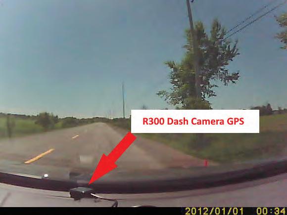
A high-performance racing GPS, the Qstarz BT-Q1000eX GPS lap timer recorded the vehicle movement, as did a R300 dash camera GPS module. After testing, the data from both devices were recovered and position information was imported into Google Earth to review the ground traces. Testing was captured by both GPS units, but it was evident that the BT-Q1000eX was higher resolution and precision. Speed information was exported to Excel for further analysis and comparison.

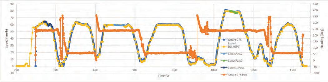
Although it was understood that the capabilities of the R300 dash camera GPS would be limited, it served to validate the data collected by the BT-Q1000eX. With the velocity plots aligned, the accelerations and decelerations showed a high degree of correlation. Both GPS units showed similar velocity ranges over the testing timeframe.

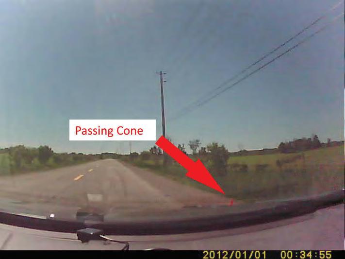
Traffic cones were placed at 20m intervals down the right side of the roadway. Velocity was calculated using the timing that each cone passed by the vehicle in the dash camera video. These speeds validated the speeds from both GPS receivers in an independent manner.

Video Velocity Analysis

A dash camera attached to the center of the windshield successfully recorded all the testing. Several passes down the road were chosen for video velocity analysis.

Accurate times were needed for each frame before velocities could be calculated. The data embedded in the video suggested it had a frame rate of 30.00030 frames per second. Duplicate frames were found and deleted. Once the duplicates were removed and the frames renumbered consecutively, frame rate analysis was conducted. A unique frame rate of 24.95 frames per second was calculated. With this value, each frame represented a time interval of 1/24.95 = 0.04 seconds. Similar frame rate measurements were conducted on the second and third pass clips. The results were 24.98 and 24.97 frames per second respectively.

In order to compare methods, lens distortion was estimated in two different ways. For the first pass, a multiple reference straight line adjustment was made. For the second and third passes, a calibration grid was filmed and detailed distortion analysis was conducted on the footage.

Identifiable features in the imagery were designated and tracked for as long as possible. These trackers were also identified in Google Earth, and corresponding UTM coordinates were transcribed. The location information was imported back into video analysis software so that it could determine where the dash camera was located and how it was oriented for each frame of video.

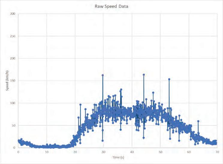
The dash camera position information was matched with estimated timings for the corresponding frames, and velocities were calculated in the X (N-S) and Y (E-W) directions. These velocities were added together in order to estimate speeds down the road. The results were plotted against time to show the acceleration profile.

Cubic spline interpolation was used to smooth the unrealistically noisy data. This method employs an elastic coefficient that strikes a balance between keeping the curve shape and reducing spurious data. Goodness of fit statistics can be calculated on the curve, and reasonable values sampled for the required range. The spline interpolation has the effect of improving the data to reflect real constraints such as vehicle limitations on vertical and lateral movement.

The combined X and Y data for the first speed pass were imported into mathematical analysis software. Fitting a spline onto the data with a smoothing parameter of 0.08 produced a plot that clearly kept the curve shape but eliminated spurious fluctuations. Spline fits were also produced for the other two passes.

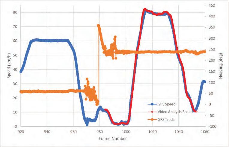
Plotting the velocity data from the primary sources, there appeared to be very strong agreement between the analysis and truth data. Minor fluctuations were visible in the dash velocity plots.

Examining all three passes together, the velocity analysis very closely matched the underlying 10Hz GPS data, both at 60 km/h and 80 km/h. The acceleration and deceleration were captured each time, and only minor variations were noted. The overall analysis suggested that the dash camera video analysis process described in this report produced speeds within 2 km/h of the true speeds.

Findings

Over the course of the video analysis, several things were found based on the dash camera video footage from Leitrim Road: a. Analysis of the test vehicle dash camera video suggested that it accelerated to a maximum of 60 km/h on the first pass, 60 km/h on the second pass, and 80 km/h on the third pass. b. Vehicle deceleration was accurately captured on all three passes, and acceleration was also captured on the third pass analysis. c. The velocities produced through dash camera analysis were commensurate with truth data captured by a high-performance GPS speed logger, generally within 2 km/h.

Conclusions

The dash camera analysis yielded velocity data that was very much in agreement with the high-performance GPS data. This suggests that accurate and useful speed information can be extracted from video, even if an onsite survey is unavailable. Analysis is not limited to investigators in the vicinity of the accident site, but can be conducted by experts from around the globe.

Video has typically been seen as qualitative evidence for traffic accident collision reconstruction. This and previous testing has shown that when properly analyzed, video can reveal accurate quantitative data as well. Despite being a relatively new capability, video velocity analysis has been used in several court cases and at this point in time has not been contested.

Video Forensic Examiner

The video forensic examiner and author of this report is Mr Adam Cybanski, a qualified accident investigator and video velocity specialist that has been leading the industry in analysis of video for velocity. Mr Cybanski holds a BSc in Computer Mathematics and gained his Investigator In Charge level 3 in 2012 at the Directorate of Flight Safety in Ottawa, Canada. Mr Cybanski has also studied photogrammetry and traffic accident reconstruction. Throughout his years of experience Mr Cybanski worked on velocity and motion extraction from video on a professional level within the aircraft and traffic accident investigation communities domestically and internationally. As founder of Gyro Flight and Safety Analysis Inc., his key responsibilities over the past five years included: audio analysis, video analysis, velocity extraction, accident reconstruction, accident visualization, accident site 3D modeling and employment of UAVs to support accident investigation. Mr. Cybanski has been recognized in court as an expert in the field of Video Velocity Analysis.

Gyro Flight and Safety Analysis Inc. provides expert video analysis and accident reconstruction services in the areas of video forensics and velocity extraction from video. Based in Ottawa, Canada, it offers an impartial, independent and specialised service to police, military and civilian prosecution and defence. The company adheres to a strict nondisclosure policy in relation to all case files worked on and abide by the APCO guidelines and the Data Protection Act 1998.

A. Cybanski BSc, IIC3 CEO Gyro Flight & Safety Analysis Inc. cybanski@gyrosafety.com

The above person – hereinafter to be referred to as ‘the person concerned’ – maintained strict confidentiality of all of the information and insights he had obtained in respect of the investigation referred to above until it was cleared for release.

Annex A Velocity Reference Data Overview

The author drove a sedan down a nearby roadway at different speeds. Their passes were recorded with an onboard dash camera. In order to assess the accuracy of derived dash camera video velocity analysis, GPS data was also collected from two onboard receivers.

A standalone Qstarz BT-Q1000eX GPS lap timer, and a R300 dash camera GPS both recorded the speed testing. After the testing, the data was downloaded from both devices and reviewed in the associated software applications. The data was subsequently exported to Google Earth, where the track could be overlaid on the actual roadways to verify the validity of the data. Qstarz data including speed could be exported into Excel for subsequent review, but the dash camera GPS speed information had to be transcribed from the dash camera playback, as the application could not export anything other than position information. Velocity data from both GPS units on the analyzed speed run was compared.

Traffic cones were placed at 20m intervals down the right side of the roadway. Velocity was calculated using the timing that each cone passed by the vehicle in the dash camera video. These speeds were employed to validate the speeds from both GPS receivers in an independent manner.

Speed Passes

Once cones were placed on the roadway, the test vehicle (a 2013 Hyundai Sonata) was positioned on the north side of the road heading southwest. The GPS and dash camera were confirmed on and running, then the vehicle accelerated to 60 km/h with reference to the automobile speedometer. The goal was to attain this reference speed prior to reaching the traffic cones, and maintain the speed until the cones were no longer visible.

After the first pass, the test vehicle was driven back to the starting position, the equipment checked, then a second test pass was conducted, again to 60 km/h with reference to the speedometer. The automobile returned for a third and final pass, this time at 80 km/h. Once the passes were completed, the GPS and dash camera were switched off, and the cones were retrieved.

Qstarz BT-Q1000eX GPS

The primary GPS reference was the BT-Q1000eX made by Qstarz. It is designed for logging speeds for extreme sports, specifically super moto, road course motorcycles, oval or road course autos. It is easy to use with a simple on-off activation switch. The GPS is a powerful 10Hz data logger with 8MB memory size able to log up to 400,000 waypoints with a 42-hour battery life.

The BT-Q1000eX employs the MTK II chipset with high sensitivity -165dBm and 66 channel tracking. It has a built-in patch antenna with LNA an L1 frequency of 1575.42MHz and C/A Code 1.023MHz chip rate. The stated accuracy is 3.0m 2D-RMS <3m CEP(50%) without SA (horizontal) and a velocity accuracy of 0.1m/s without DGPS aid.

Once testing was completed, data was downloaded from the GPS into the supporting software, Qstarz – QRacing Version 3.60.000 Build Date 8 June 2016. The track was subsequently exported as gpx, Excel csv and Google kml files. The Excel file was comprehensive, providing an index, UTC and local times to the second, time in milliseconds, latitude, longitude, altitude, speed and heading information every one tenth of a second. The track started at 17:37:51 UTC on 19 June 2018, and ended at 18:04:16

UTC on the same day. In total, 15,403 samples were recorded during the testing period.

QRacing saved the gpx data into a 6.7MB kml file employing gpx2kml.com conversion. The track captured by the BT-Q1000eX matched the Google Earth imagery nicely, and exhibited significant resolution that clearly discerned the individual passes down Leitrim Road.

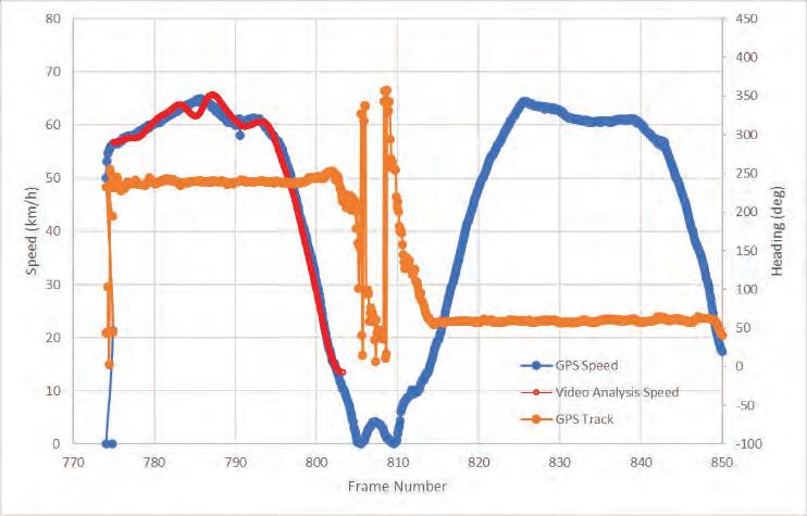
The testing runs needed to be identified in the data. Although the GPS recorded 26 minutes of data, the three passes took less than 15 seconds each. The relevant passes were identified by the speed and track plots. Plotting the speed showed a smooth, high resolution (10 Hz) graph that depicted six peaks in speed. These peaks represented the three logged East to West speed passes, along with the return route back to the starting point. This was verified by the alternating GPS tracks of 60 and 240 degrees. Time was measured in seconds from the point where the vehicle first started moving. The GPS-calculated speed was in km/h.

R300 Dash Camera GPS

The back-up GPS reference was the R300 external GPS unit for the dash camera. It is an add-on for a low-cost dash camera, and very little information about it was available. The unit attaches to the camera with a long cord. Once plugged in, position data is encoded into the dash camera video, and can be extracted using the supporting software.

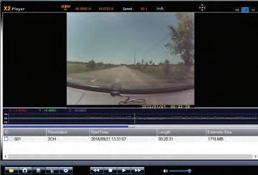
Testing was conducted with the R300 dash camera attached to the windshield, and the GPS attachment tethered to the camera. The resulting video was called G2012-01-01-0024-57.avi. In order to access the embedded GPS data, the file had to be opened in the software application X2Player. exe, version 2.5.6.0 dated 2014-07-04 12:14 PM. The software allows the user to review the forward and backward camera footage with typical VCR controls. If the GPS module was attached during recording, the software will also display the instantaneous latitude, longitude, and speed in orange at the top of the screen.

measurement devices, the BT-Q1000eX could be used as velocity truth data with confidence.

Visual Measured Reference Speed Analysis

To provide a non-GPS confirmation of reference speeds, eleven orange cones were placed down the right side of the roadway at 20m intervals. On the shoulder of the road, they could be seen passing by the front of the vehicle in the dash camera footage.

The velocity information could not be directly exported from the application. In order to extract this information, the sequence was played back in the interface software and recorded onto video. On review, all distinct changes in velocity were transcribed, along with the corresponding dash camera time stamp. This produced a course plot very similar to the BT-Q1000eX.

Although it was understood that the capabilities of the R300 dash camera GPS would be limited, it served to validate the data collected by the BT-Q1000eX. Once the velocity plots were aligned they showed a high degree of correlation in both acceleration and deceleration. Both GPS units showed similar velocity ranges, over the testing timeframe. With two independent agreeing velocity

By noting the frame number and timestamp as each cone left the view over the vehicle dash, and knowing the distance between each cone, the speed of the vehicle could be calculated using cubic spline interpolation. Speeds near 60 km/h for the first pass, 60 km/h for the second pass, and 80 km/h for the third resulted. The speeds at each cone passage were plotted along with the previous GPS data, and matched well, supporting the BT-Q1000ex speeds.

Speed Comparison

The 10Hz data logger GPS provided the highest resolution data, and appeared very accurate. It did not provide any data during the first pass acceleration, perhaps because it had not yet locked enough satellites, but worked well for the remainder of the testing. The dash camera GPS produced speeds at a relatively low 1 Hz, but closely aligned with the 10Hz GPS speeds. The calculations from the cone passing were of a very short duration, but again reflected the same speeds obtained from the GPS units. Comparing the data from the two GPS units and the speeds obtained through passage of the reference cones, a very high confidence was placed in the 10Hz GPS data for the purposes of this testing.

Summary

Speed data was collected from two independent GPS sources and by timing the passage of cones placed at measured distances. All three sources agreed, although the BT-Q1000eX provided much better temporal resolution at 10 position readings per second. The associated speed calculations were employed as truth values for comparison with dash camera video velocity analysis.

Annex B Dash Camera Analysis Overview

An inexpensive dash camera was affixed to the test vehicle windshield in order to record the testing. The resulting video was subsequently downloaded off the camera. Three passes down the road were chosen for velocity analysis. The sequence was broken down into individual images which were sequentially numbered and documented. Duplicate frames were noted and removed.

The imagery underwent geoidentification. Identifiable features were designated and tracked. These features were also identified in Google Earth, and corresponding UTM coordinates were noted for each. Other distinct features were also manually tracked.

The video sequences were matchmoved to derive camera/ vehicle position. The On Screen Display (OSD) time information from each frame was transcribed, and compared to the frame rate timing. Distinct time values were calculated for each frame. The derived position and time information were matched and used to calculate velocity for each frame of the test passes.

R300 Dash Camera

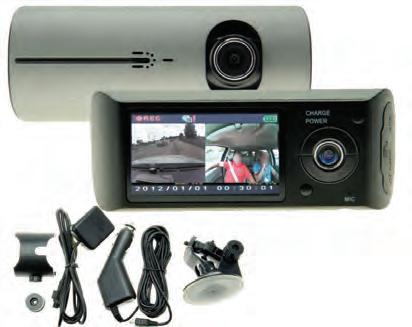
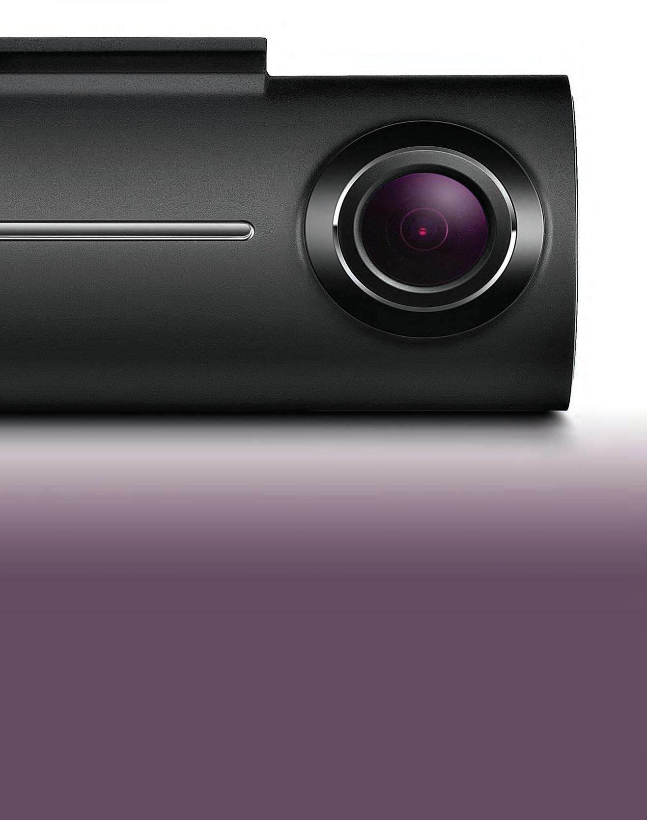
The R300 is an inexpensive and widely available Dash Camera that was purchased off of eBay. It was bought on February 2016 for $50USD, and as of the time of this article is still available for purchase. Although it cannot be considered high quality, its output was seen as being representative of the type of dash camera footage that could be available from an accident.

The dash camera has a 2.7” LCD screen on the back, a G-Sensor, a microphone to capture cabin audio, and an external tethered GPS module. A front 140-degree wide angle lens captures video at 640x480 resolution, while a rear-facing 120-degree lens can also capture video at the same resolution. The camera includes a 12V adapter to power the unit, and a windshield mount.

The dash camera was mounted in the center of the windshield for testing. Power was applied, and the unit continuously recorded video until the vehicle returned and the dash camera was shut off. The result was an avi video file, titled G2012-01-01-00-24-57. The video ran for 15 minutes and 40 seconds. The associated file size was 1.17GB, recorded on a 32GB microSD card.

The videos were opened in VLC media player in order to view the codec information. The video codec was Motion JPEG Video (MJPG) with a resolution of 1280x480. The front camera imagery was on the left side of the frame, 640 pixels wide, while the rear camera view was shown on the right. The indicated frame rate was 30.000300, and the decoded format was Planar 4:2:2 YUV full scale. Audio was mono PCM S16 LE (araw) with a sample rate of 16160 Hz and 16 bits per sample.

The footage was reviewed. The first suitable sequence for video velocity analysis was at dash camera time 00:30:45. This segment started with the vehicle accelerating from the right side of the road, moving left into the traffic lane, going by the orange test cones, then decelerating. It fit well with the type of dash camera video that might be collected from an accident, and also captured significant acceleration which can be more difficult to derive speeds for.

An additional two sequences were selected for dash camera video analysis, all starting from the same general area. The second sequence started at 00:32:05, and the third started at 00:34:15.

Individual png frames were extracted from G2012-01-0100-24-57 starting at 00:24:57 and they were sequentially named frame0000.png to frame28168.png. The images were cropped on the left, to only show the front camera view and not the back camera. Three subsets of the images were set aside, representing the three test passes. The new sequences were reviewed frame by frame, and any duplicates (identified by a lack of movement), were deleted. The OSD time for each frame, along with its unique frame number were transcribed into Excel for subsequent temporal analysis. The frames were then renumbered so that the sequence again began at Frame0000.png, but this time at dash camera times 00:30:45, 00:32:05 and 00:34:15. The result was continuously numbered sequences of unique images covering the three test runs.

Temporal Analysis

Accurate times were needed for each frame before velocities could be calculated. The data embedded into the video suggested it had a frame rate of 30.00030 frames per second. By closely examining the OSD timings, this could be verified. The OSD time changed from 00:24:57 to 00:24:58 at frame00032. It changed from 00:40:33 to 00:40:34 at frame28110. Over the 936 second period, there were 28078 frames, resulting in a calculated frame rate of 28078/936= 30.0 frames per second

The calculated 30 frames per second does not tell the whole story, as duplicate frames were found and deleted prior to analysis. Once the duplicates were removed and the frames renumbered consecutively, the same sort of frame rate analysis was conducted. The OSD transitioned to 00:30:46 at frame 25, then transitioned later to 00:31:06 at frame 524. This was found to represent a rate of (52425)/20=24.95 frames per second, the unique frame rate. With this value, each frame represented a time interval of 1/24.95 = 0.04 seconds.

The final frame timings were not yet complete. As stated, there were duplicate frames which had to be removed before analysis could be carried out. With five duplicate frames per second, the question was whether the duplicates were evenly spaced and each image recorded with a 1/25 second interval, or if the images were recorded with a 1/30 second interval, followed by an extra interval after every 5th image. Previous testing had confirmed that the initial scenario, with a constant frame rate of 24.95 frames per second was correct.

Similar frame rate measurements were conducted on the second and third pass clips. The results were 24.98 and 24.97 frames per second respectively.

Lens distortion analysis

In order to compare methods, lens distortion was estimated in two different ways. For the first pass, a multiple reference straight line adjustment was made. For the second and third passes, a calibration grid was filmed and detailed distortion calculated from the result.

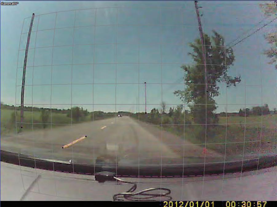
For the first pass, a frame showing three telephone poles and the bottom dash line were selected at a point just prior to pole passage by the vehicle. The frame exhibited significant curvature for the nearby poles and the dashboard. A straight line was drawn from the bottom to the top of each pole, and the quadratic lens distortion coefficient was adjusted until the lines showed approximately the same amount of curvature as the poles and dash. This yielded a quadratic distortion of -0.06300, and was employed for subsequent analysis of the first pass.

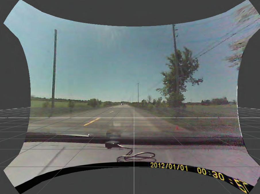
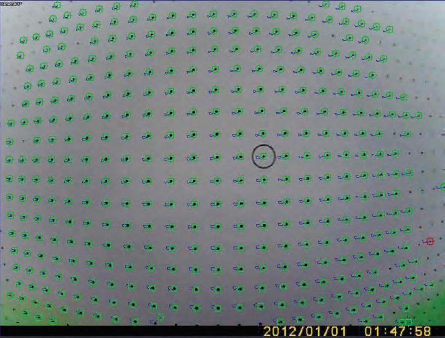
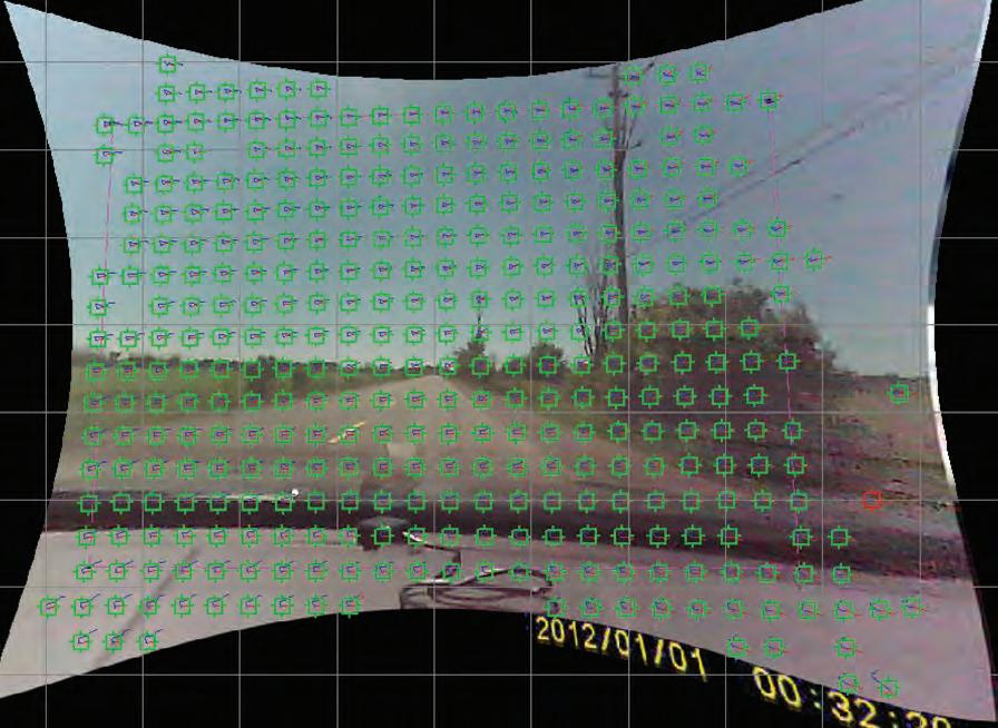
For the second and third passes, a calibration grid was printed, filmed, then employed for more accurate lens distortion analysis. The 8” x 10” sheet of equally-spaced dots were filmed on the dash camera for two seconds. This footage was extracted from the camera and imported into SynthEyes. Lens grid trackers were created, tracked through the duration of the video, corrected if they ran off, then processed. The resulting distortion map was saved and employed in the analysis of passes two and three. While the straight-line adjustment lens distortion analysis showed unrealistic square corners in the perspective view, the auto-calibration showed more realistic curved distortion, likely indicative of a more accurate lens distortion analysis.

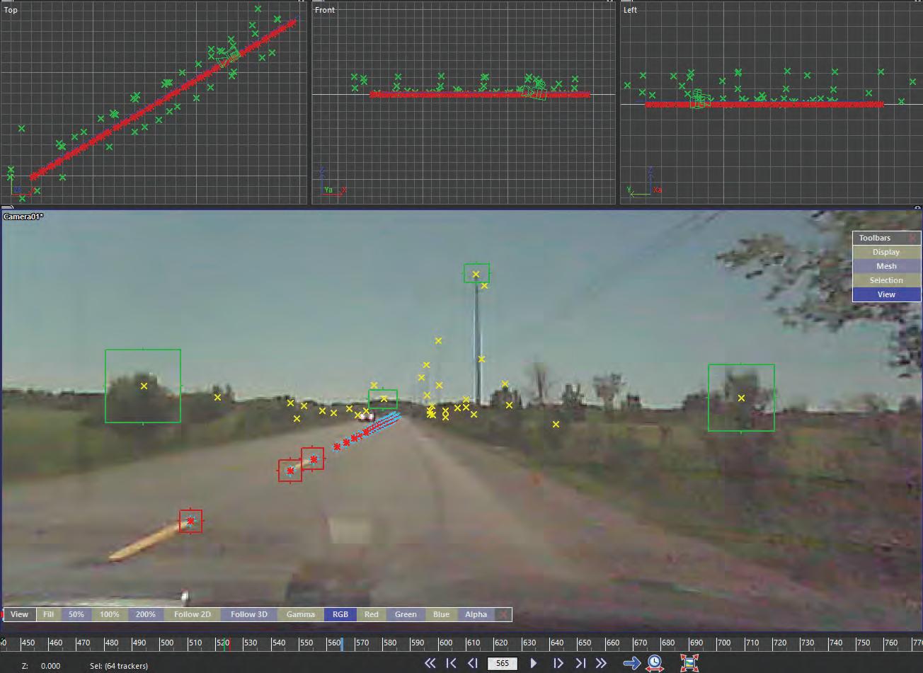
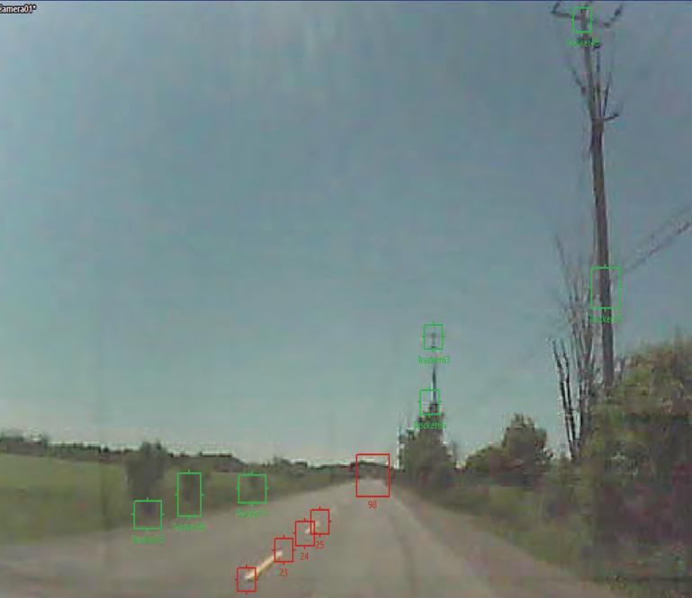
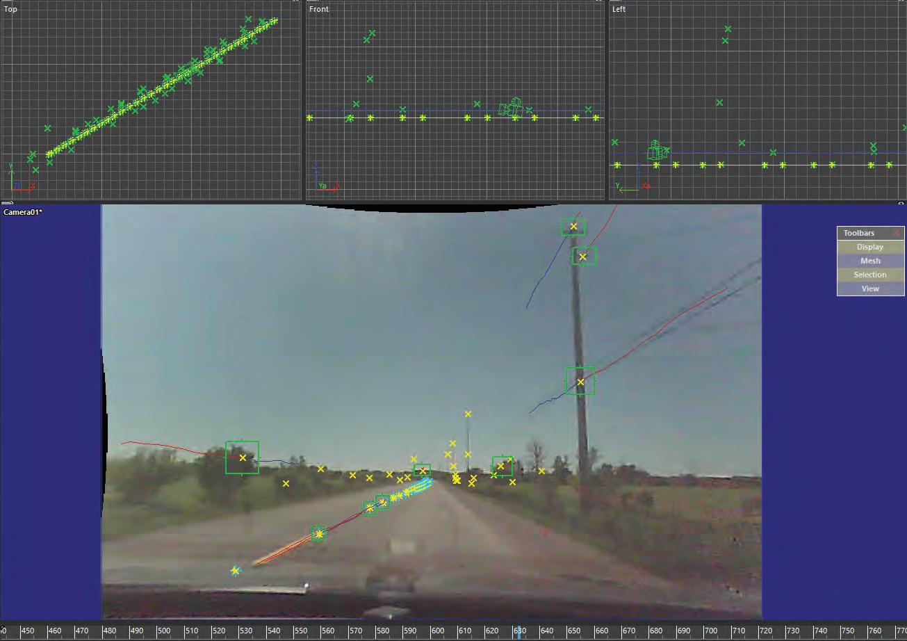
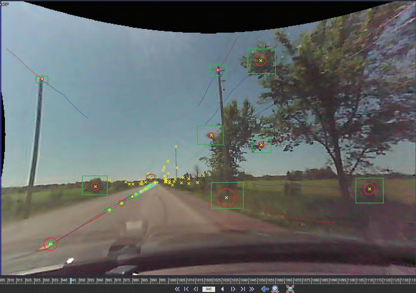
The first image sequence was loaded into SynthEyes and the video reviewed for suitable ground tracking references. A total of 100 distinct features on the ground were designated, that could also be positively identified in Google Earth. They were labelled sequentially starting at Tracker 1. Each feature was manually tracked in the reverse direction so that they could be followed as long as possible. Road trackers consisted predominantly of dashed roadway lines, along with a couple of other lines and poles. These trackers would be used as references to geolocate the camera.

The road trackers were augmented by 22 other distinct objects visible in the video, such as telephone poles tree branches and bushes. Although they could not be used to geolocate the camera because precise 3D coordinates were not available, they were useful as stationary visual references and helped the software distinguish the movement of the camera. All the feature tracking was reviewed with trackers trails and in graph view in order to identify and correct any tracking mistakes or inaccuracies. The end result was a cloud of trackers that were consistent with the dash camera motion.

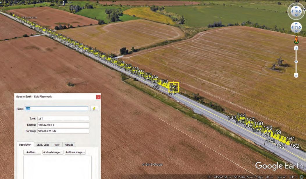
Each tracked road feature was identified in Google Earth, and a placemark carefully positioned on the surface of the roadway. Although it varied with the type and clarity of the feature, the horizontal position of each feature could be discerned to a few centimetres, more than accurate enough for vehicle velocity calculations. The UTM coordinates for each were obtained and transcribed. These georeferenced road features were collected into a file that could be imported into SynthEyes as known lock points.

Once the road tracker locations were designated in SynthEyes, they were viewed in a top-down perspective. The dispersion of the trackers in SynthEyes matched those in

Google Earth with no outliers. With a verified group of reference trackers, matchmoving could start. In this case, the roadway was relatively flat, and an estimated height of zero was used for all road tracker heights.

For the first pass, which employed a simple curved line adjustment for camera distortion, the camera solve resulted in an error of just over 5 pixels. Error cannot be measured in physical units such as metres or centimetres in matchmoving, because an object that is 2 pixels wide could be very small if it is near the camera (such as a crack in the roadway), or very large if it is far away (like a tree in the distance). From experience, the error should be less than 1 pixel if the matchmoving is being done for filmmaking, but can be between much higher (5 or greater) for velocity analysis purposes.

For each sequence, the software was able to figure out where the camera had to be in relation to the ground trackers, how far above the ground, and where the camera was pointed (pitch, roll, and heading) in order for the solved camera to match what was seen in the video. The software also estimated what the camera focal length was, and for this project the calculated value was approximately 7 mm. Once solved, the application was able to show exactly where the camera was and how it was oriented for each frame of video, both graphically from different perspectives (top, front, left), and numerically.

The camera position information was carefully reviewed to make sure it made sense. It showed the camera as travelling to the right of the roadway line. The calculated height above ground was approximately 1m, which is reasonable for a dash camera mounted on the windshield of a sedan. The orientation information indicated that the camera was mounted level, pointed on an upward angle of 4 degrees, and oriented towards a heading of 243 degrees as it travelled down the road initially. A quick check in Google Earth showed that the orientation of that section of the road was 239 degrees, so with the camera oriented forwards in the sedan, it could certainly have been pointed 4 degrees right of centre, resulting in the 243-degree heading. The camera solves appeared reasonable.

The next step was to combine the timing and distance data in order to derive velocity. The camera X and Y positions from the solve were exported into Excel, and matched with the corresponding time data. Prior to additional data analysis, a rough velocity plot was assembled.

At 60 km/h, the vehicle moves approximately 0.7m per frame (0.04s). At slower speeds, it moves less. Over the time range 0-20 seconds, when the test vehicle was travelling at approximately 60 km/h, the matchmoving process calculated that the vehicle moved an average of 0.702m. Over this range, the minimum was 0.12m and the maximum was 6.5m. The variation is due to a number of rea- sons including the low resolution of the video, changing trackers in different positions, and dispersion of the trackers. Calculating the instantaneous speed from these values showed large fluctuations, but a very discernable trend.

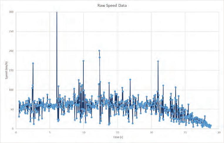
This variation in distance travelled results in significant variations in calculated velocity, when the distance is measured over just 0.04s. One way to improve the velocity precision is to increase the sample size, or measure distance travelled over a longer time such as a quarter, half, or even one second. The disadvantage of this is that useful data is being thrown away. When a one-second interval is used, 24 other measurements between the first and last value are ignored. The result is a single velocity value, and no acceleration/deceleration data during that one second period. In addition, if the one distance value used for measurement happens to be an outlier, the velocity at that point will be skewed.

A better way to employ the data is to use cubic spline interpolation. This method employs a virtual elastic ruler to join the sample points. The ruler is attached to the first point, then stretched through each point to the last, making a cohesive curve. The tightness of the elastic can be decreased or increased, taking it from the raw data through different levels of smoothness, all the way to a straight line. Once an elastic coefficient is chosen that strikes a balance between keeping the curve shape and reducing spurious data, goodness of fit statistics can be calculated on the curve, and reasonable values sampled for the required range.

The spline interpolation has the effect of improving the data to reflect real constraints. SynthEyes solves the camera location and orientation separately for each frame of video. As a result, the camera (and vehicle) varies in position as a result of error. The actual vehicle cannot jump laterally, because of the friction of the tires on the road. Any changes in lateral position will be smooth as the vehicle drives forward. Similarly, the vehicle cannot jump in the longitudinal axis, because of tire friction and inertia. As a result, the true vehicle track in the lateral and longitudinal axis would be smooth, similar to a cubic spline, and not noisy like the raw data.

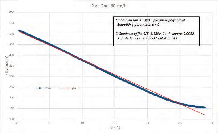
The combined X and Y data were imported into mathematical analysis software. With a smoothing parameter of zero, the fit is a straight line. The resulting Sum of the Squares Error (SSE) is very high at 6.189 e+04, and the R-square error is below 1 at 0.9932. The R-Square error is still relatively close to one because the data curve itself is quite straight. This value would decrease if there was a much greater change in velocity over the time.

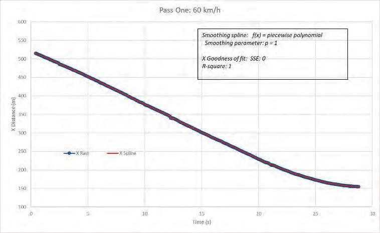
Once the smoothing parameter is increased to the maximum of 1, the fit exactly reflects the data, with every bump and variation. The Sum of the Squares Error decreases to zero, and the R-Square increases to 1. This is a perfect fit of the data, but the variation/noise in the graph does not reflect the actual vehicle motion. A lower smoothing value is needed.

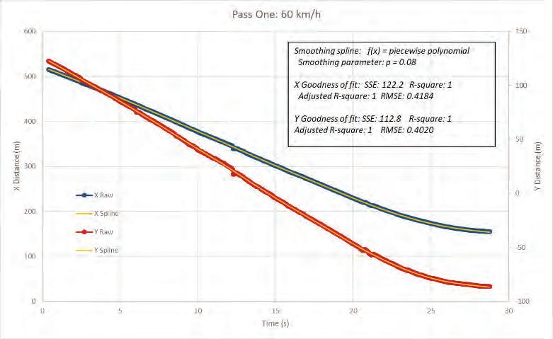
A data set was produced with time on the horizontal axis and both X and Y distances on the vertical. Fitting a spline onto the data with a smoothing parameter of 0.08 produced a plot that clearly kept the curve shape, but eliminated spurious fluctuations. The calculated RMSE were 0.4184 and 0.4020, while the R-square was one, suggesting good fits.

The 1st derivative of distance (in metres) and time (in seconds) produced velocity data in m/s for each frame of video. With the X (or N/S) and Y (E/W) velocity informa- tion, the speed down the road could be calculated by the square root sum of the squares of each X and Y velocity component. These instantaneous velocities were multiplied by 3600 and divided by 1000 to change the units from m/s to km/h. The resulting data was aligned with the previously calculated speed truth data and plotted.

The derived video analysis speed data reflected the underlying GPS speed data well. The speed climbed from 57 km/h to a maximum near 65, then fell to 60, stabilized for a short period, then bled off to 15 km/h. The derived speeds did not vary from the truth data by more than 3 km/h, and was for the most part within 1 km/h. It captured both the acceleration and deceleration well. The slight inconsistency just prior to the maximum speed could have been the result of the relatively high camera solve error. Better lens distortion analysis would have helped address this.

Second Test Pass

For the second pass which employed the lens grid autocalibration for camera distortion, the camera solve resulted in an error of 1.06 pixels, a very low and accurate value. The camera movement looked smooth in playback, again travelling to the right of the roadway line. The software estimated the camera focal length at 22mm, a narrower field of view than the previous pass due to the cropping of the lens distortion correction. The calculated height above ground was approximately 1.1 m, and the orientation information indicated that the camera was tilted 6 degrees to the left, pointed on an upward angle of 5 degrees, and oriented towards a heading of 238 degrees as it travelled down the road initially.

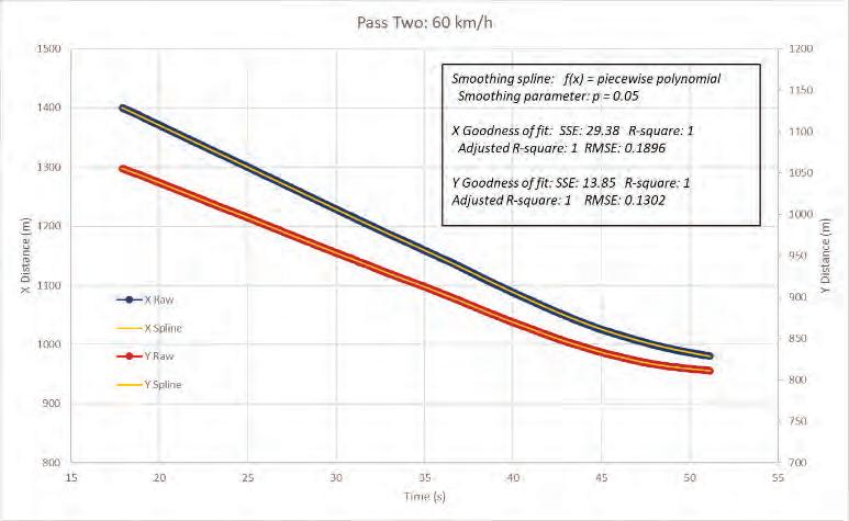
A data set was produced with time on the horizontal axis and both X and Y distances on the vertical. Fitting a spline onto the data with a smoothing parameter of 0.05 produced a plot that clearly kept the curve shape, but eliminated spurious fluctuations. The calculated RMSE were 0.1896 and 0.1302, while the R-square was one, suggesting very good fits.

The 1st derivative of distance (in metres) and time (in seconds) produced velocity data in m/s for each frame of video. With the X (or N/S) and Y (E/W) velocity information, the speed down the road could be calculated by the square root sum of the squares of each X and Y velocity component. These instantaneous velocities were multiplied by 3600 and divided by 1000 to change the units from m/s to km/h. The resulting data was aligned with the previously calculated speed truth data and plotted.

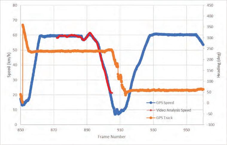
The second pass speed data again reflected the underlying GPS speed data well. The speed measurement started near 60 km/h, was relatively stable with the exception of a short decrease then increase near the end of the pass, then bled off to 20 km/h. The derived speeds did not vary from the truth data by more than 2 km/h. It captured the speed bump and deceleration.

For the third pass which also employed the lens grid autocalibration for camera distortion, the camera solve resulted in an error of 1.01 pixels, a very low and accurate value. The camera movement looked smooth in playback, again travelling to the right of the roadway line. The software estimated the camera focal length at 7mm, similar to the first pass. The calculated height above ground was approximately 1.1m, and the orientation information indicated that the camera was tilted 4 degrees to the right, pointed on an upward angle of 13 degrees, and oriented towards a heading of 255 degrees as it travelled down the road.

Once again, the raw speed values were calculated and plotted. Employing the more accurate lens distortion, and resulting low solve error, the variation in raw speed seemed lower than the previous calculated for the first pass. While there were a few outliers, the data was very close to a solid line when speed was low, and varied by approximately 20 km/h at higher speeds. The first pass showed similar variation at 60 km/h, but with significantly more outliers.

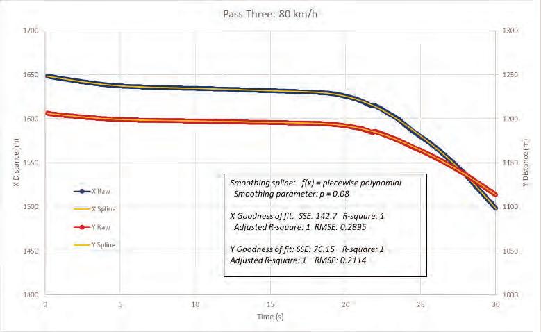
A data set was produced with time on the horizontal axis and both X and Y distances on the vertical. Fitting a spline onto the data with a smoothing parameter of 0.08 produced a plot that clearly kept the curve shape, but eliminated spurious fluctuations. The calculated RMSE were very low values of 0.2895 and 0.2114, while the R-square was one, suggesting good fits.

The 1st derivative of distance (in metres) and time (in seconds) produced velocity data in m/s for each frame of video. With the X (or N/S) and Y (E/W) velocity information, the speed down the road could be calculated by the square root sum of the squares of each X and Y velocity component. These instantaneous velocities were multiplied by 3600 and divided by 1000 to change the units from m/s to km/h. The resulting data was aligned with the previously calculated speed truth data and plotted.

The derived video analysis speed data reflected the underlying GPS speed data very well. The speed started near 10 km/h, fell to near zero, then accelerated quickly to a maximum near 80 km/h. After a short period with slight deceleration, the derived speed fell to 10 km/h. The derived speeds did not vary from the truth data by more than 2 km/h, and was for the most part within 1 km/h. It captured both acceleration and deceleration well.

Examining all three passes together, the velocity analysis very closely matched the underlying 10Hz GPS data, both at 60 km/h and 80 km/h. The acceleration and deceleration were captured each time, and only minor variations were noted. The overall analysis suggested that the dash camera video analysis process described in this report produced speeds within 2 km/h of the true speeds.

Summary

The dash camera is a low-cost imaging device easily accessible to the general public, not a high-precision instrument. The limited resolution of 640x480 on the video hampered the analysis and results. Even with this limitation, dash camera video velocity analysis was able to extract precise high-resolution velocity data from the image sequence. This data was compared to a high sample rate GPS designed to accurately measure speeds for racing, and found to be comparable. Dash camera video velocity analysis has proven to be a precise and useful capability for the modern accident investigator.

POWER LOSS ISSUES RELATED TO EDR DATA IN 2013-2017 KAWASAKI NINJA 300 AND ZX-6R MOTORCYCLES

Starting in 2013 Kawasaki Heavy Industries, Ltd. (KHI) has installed Event Data Recorders (EDR) on select US sold motorcycles. The two motorcycles covered in 2013 are the Ninja 300 and the ZX-6R. On both these models an EDR event is triggered when the motorcycle is tipped over and goes into an emergency shutdown (ES). The emergency shutdown is a safety feature that involves shutting off the fuel pump relay, fuel injectors, and ignition system when the motorcycle senses it has fallen. The rest of the electronics will remain active. Additionally, to trigger an EDR event the rear wheel must be in motion or gone through a sudden deceleration in the several seconds prior to ES. On the Ninja 300 and ZX-6R the time between tip-over and ES is approximately 1.3 seconds. However, as studies have shown this time can be significantly increased if the motorcycle is still sliding/bouncing creating considerable “noise” in the tip-over sensor. The data parameters captured in an EDR event can be seen in Table 1. In addition to the data parameters, the EDR will capture the ECU runtime and key cycles at the event, as well as the elapsed ECU runtime and key cycles since the event. 1,2

2 Hz data

Front wheel speed*

Rear wheel speed

Gear Position

Inlet Air Temperature

Coolant Temperature

Battery Voltage

DTC’s

Power (P-Mode)*

KTRC Mode*

10 Hz data

Throttle Position

Engine RPM

Clutch In/Out

Fuel Injector Pulse

Timing BTDC

Fuel Cutout

*ZX-6R only

Table 1: EDR data parameters for Ninja 300 and ZX-6R

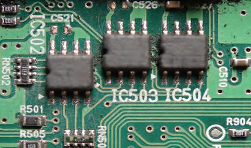
The EDR data is stored in the Engine Control Unit (ECU) on three non-volatile memory chips (EEPROMs). An image of the three EEPROMs on the Ninja 300 can be seen in Figure 1. The power supply critical to triggering and subsequently writing an EDR event to the ECU comes in two forms; switched and unswitched. The switched power comes from the ECU relay and the unswitched power comes straight from the battery. Similar to your typical automotive radio, there is a constant power feed (unswitched) which stores the clock, presets, and other user data on the radio, and a switched power feed that generally powers up the radio. The ECUs in the Ninja 300 and ZX-6R work in a very similar fashion. Both the switched and unswitched power to the ECU is necessary for the motorcycle to go into ES and trigger an EDR event. Once in ES and the EDR event is triggered, only the unswitched power is necessary to save the data to the EEPROMs.

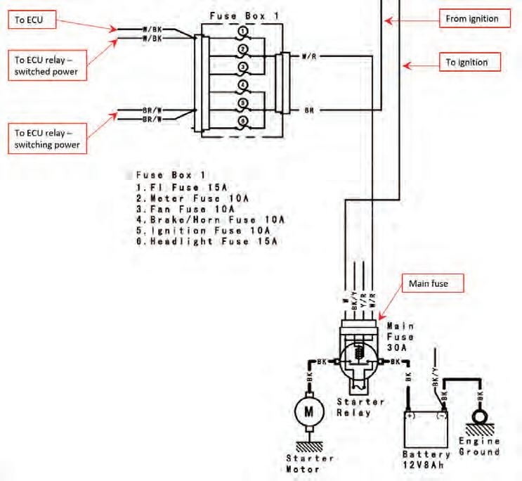
On the Ninja 300, all the motorcycle power comes through the main fuse located on the starter relay assembly (see Figure 2). From the main fuse, unswitched power is fed directly to the ECU through the fuel injection fuse. Additionally, power is fed directly to the ignition switch from the main fuse. When energized, the ignition switch powers the switched side of the fuse block. This switched side of the fuse block is responsible for energizing the ECU relay. Unfortunately, if the main fuse of the Ninja 300 is compromised, the ECU will lose both the switched and unswitched power assuming the engine has stalled. However, if the main fuse is blown or there is a sudden battery loss and the engine has not stalled, the motorcycle’s alternator power will keep the engine running and supply the switched and unswitched power to the ECU.

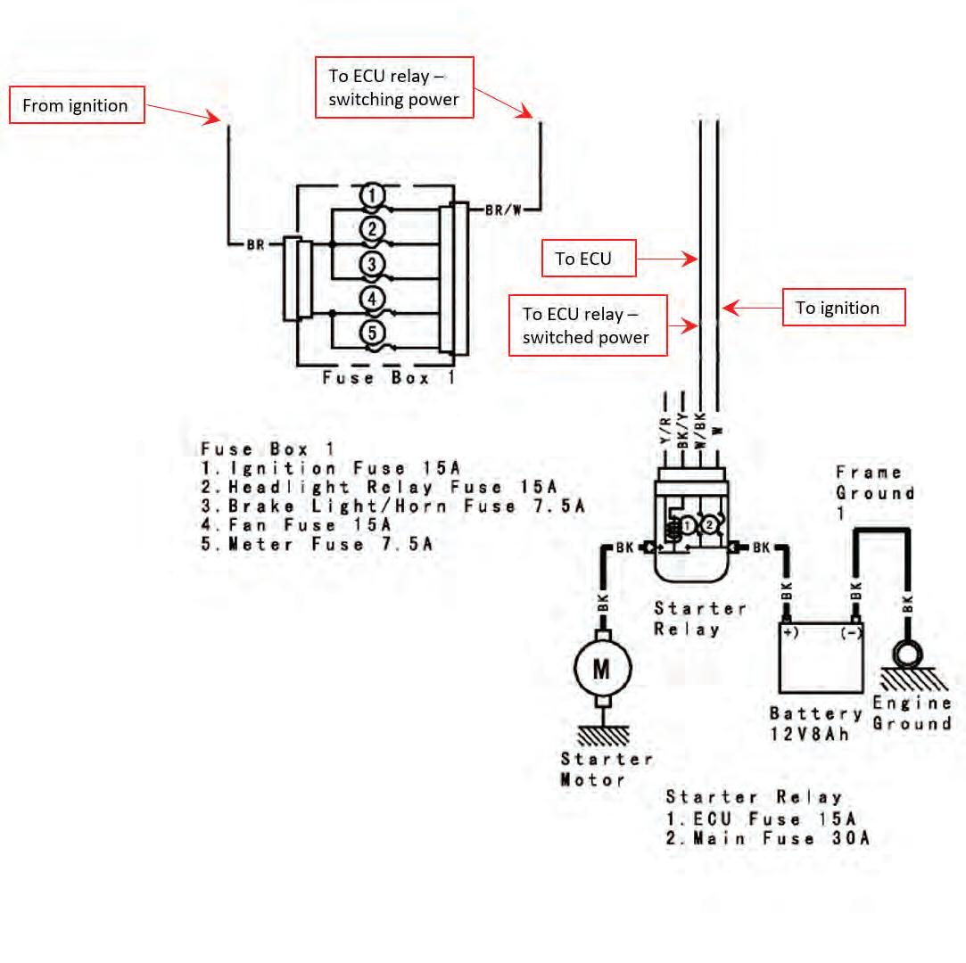
This is not entirely the case on the ZX-6R. The switched and unswitched power to the ECU is provided in a slightly different manner (see Figure 3). The ZX-6R contains two fuses incorporated into the starter relay circuit, the main fuse and the ECU fuse. A simple way of looking at it would be that the motorcycle operates using two “main” fuses. One fuse supplies power to the motorcycle and the other fuse supplies power only to the ECU. The ECU fuse is the same as the fuel injection fuse on the Ninja 300, but due to relocating it to the starter relay, it is now not reliant on the main fuse. In this case, if the main fuse blows for whatever reason, the ECU will still have its unswitched power. Similar to the Ninja 300, if the main fuse is blown or there is a sudden battery loss and the engine has not stalled, the motorcycle’s alternator power will keep the engine running. The alternator will still supply the switched and unswitched power to the ECU. However, if the ECU fuse is compromised regardless of alternator or battery power, the engine will immediately shut down.

On both the Ninja 300 and ZX-6R, if for any reason the switched or unswitched power is lost prior to ES (and assuming engine stall), no EDR event will be saved. This power loss would keep the bike from going into ES, which is necessary for an EDR even to be saved. A classic example of this would be a motorcycle colliding into another vehicle and fracturing the ignition switch or the ignition switch wiring prior to the motorcycle falling and going into ES. This is not necessarily the case if there is an unswitched power loss that occurs after the ES. Additionally, the engine stop switch (kill switch) on the handlebar has no effect on the switch or unswitched power to the ECU. The ECU can still command an ES and trigger and EDR event regardless of the stop switch position.

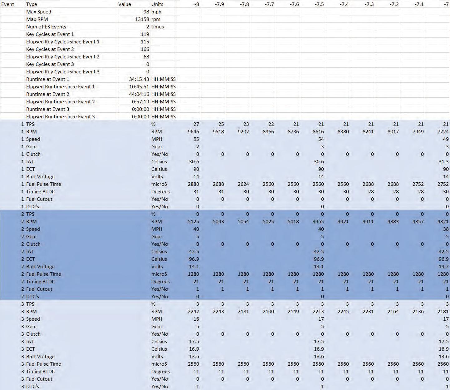
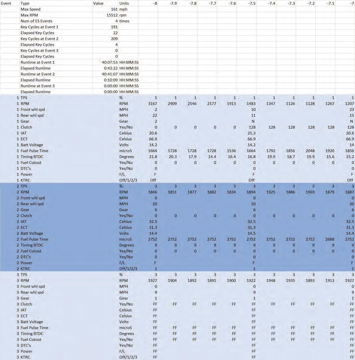
In a normal/non-power loss situation, once the motorcycle goes into ES, the ECU will write the EDR data to the nonvolatile memory. The ECU will then “wait” for the key cycle to end in order to write the appropriate ECU runtime and key cycles for that event. An example of this can be seen in Tables 2-3. Table 2 depicts a baseline download of a Ninja 300 ECU which contains two events. Table 3 depicts a test with the same ECU where the motorcycle rear wheel was elevated on a wheel stand with the motorcycle idling in 5th gear. The tip-over sensor was tilted, and the ES was commanded. Several seconds after ES with the ignition switch still on, the main fuse was pulled. As shown, the data wrote to the non-volatile memory just fine, but the ECU runtime, key cycles, and number of ES events parameters did not update. This was due to the ECU “waiting” for the key cycle to end, but it never did due to the total power loss before the key was turned off. An example of this situation occurring would be where the motorcycle falls in a low-side-type accident and slides long enough to go into ES. Subsequently, the motorcycle collides with another object severing the main fuse, fuel injection fuse or battery power (all of which provide an unswitched power loss). Similarly, if a motorcycle fell, went into ES, and was subsequently struck by another vehicle severing the main fuse, fuel injection fuse or battery power.

It is unclear as to what Kawasaki will do if this situation is present when they perform an ECU download. The author has seen in the past where KHI only provides data plots for two events. When data for only two events is supplied, it is presumed a third event never occurred. The question becomes how does KHI determine if there are only two events? If they are looking solely at the ECU runtimes and key cycles, they could overlook data present from a power loss after ES. Of note in the previous Ninja 300 example, the third event that occurred during power loss is an “unlocked” event. If the criteria are met for another EDR event, all the data in the third event will get overwritten and the ECU runtime and key cycles will populate as normal assuming no power loss issues.

This anomaly is also present on the ZX-6R. Similar to the Ninja 300, if there is unswitched power loss after ES, the event will likely be an “unlocked” event with no ECU runtime or key cycle information. On the ZX-6R the unswitched power loss would come from a blown ECU fuse or severed battery power. Remember on the ZX-6R, the unswitched power does not go through the main fuse, so compromising the main fuse would essentially yield the same result as switching the ignition off and saving an EDR event normally.

Another anomaly resulting from power loss after ES is a partial recording. As mentioned previously, once the motorcycle goes into ES, if the EDR recording criteria is met, the data will begin writing to the non-volatile memory immediately after ES. However, if the unswitched power is lost during the writing process, only part of the EDR data

When inspecting a Kawasaki motorcycle with possible EDR recording capability, be certain to inspect the ignition switch and wiring in detail

Table 3: Ninja 300 Power Loss After ES Occurrence

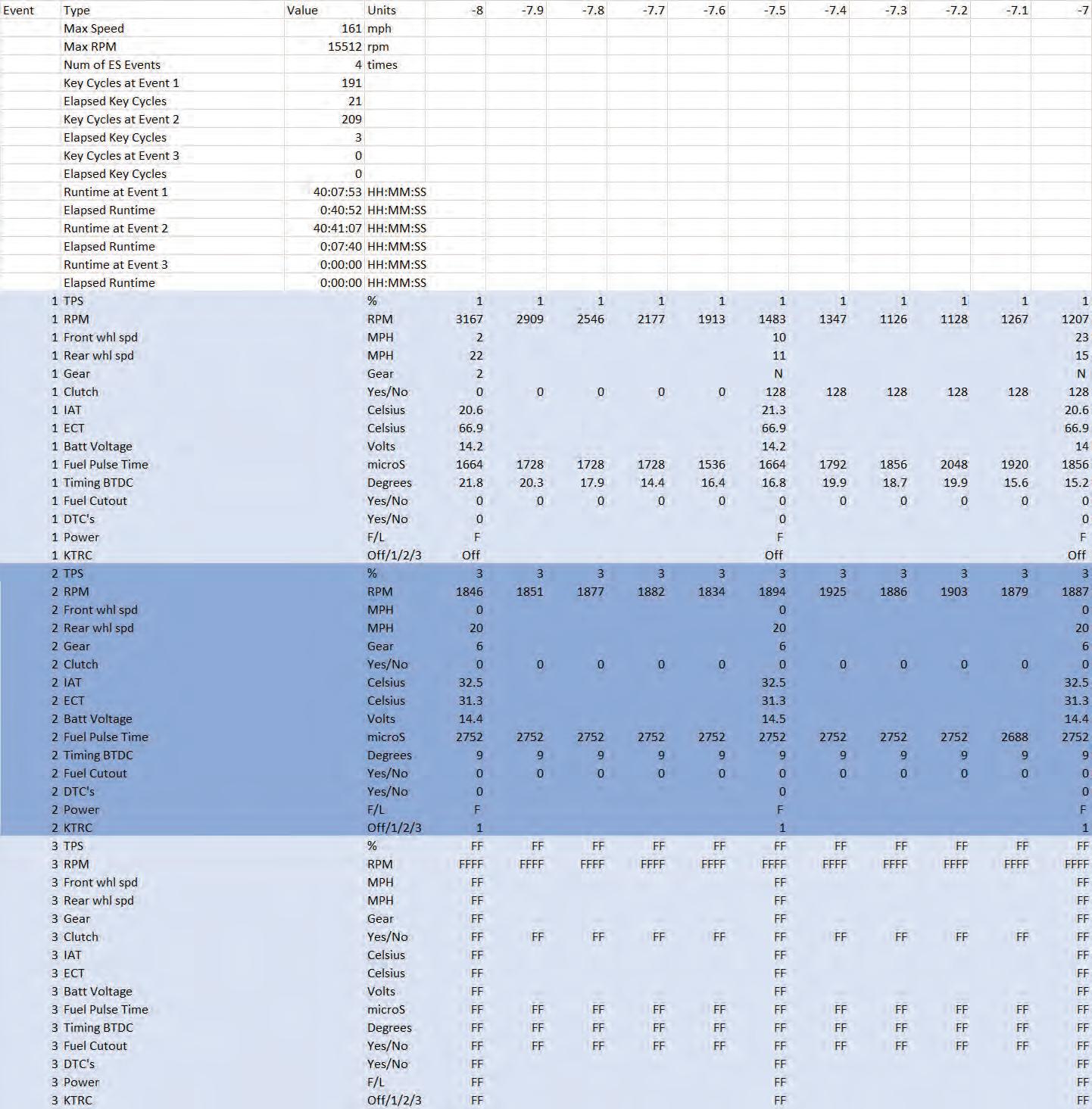
will be saved. An example of this can be seen in Tables 4-5. Table 4 depicts a baseline download of a ZX-6R ECU with two events. Table 5 depicts a test with the same ECU where the motorcycle rear wheel was elevated on a wheel stand with the motorcycle idling in 1st gear. The tip-over sensor was tilted, and the ECU fuse was pulled approximately 1.5 seconds after ES. As can be seen in the table for Event #3, the data was saved up to and including gear position. Similar to the Ninja 300 example, the ECU runtime, key cycles, and number of ES events parameters did not update, and this event is “unlocked”. It was found on several other tests performed, that nearly 4 seconds was required to save a complete EDR event.

In the unlikely event the main fuse is compromised, or the battery power becomes severed, but the motorcycle still runs up to ES, an event may still be recorded. Both the

Ninja 300 and ZX-6R will continue to run under their own power via the alternator after the main fuse or the battery power becomes severed. For example, if the main fuse on the ZX-6R is compromised and the motorcycle continues to run, the ECU will still have switched and unswitched power. Upon ES, the switched power will cease, effectively turning the ignition switch off and the ECU will save the EDR data due to the unswitched power still being supplied through the ECU fuse. Likewise, if the battery power becomes severed and the motorcycle continues to run, upon shutdown both the switched power (from the main fuse side) and the unswitched power to the ECU (through the ECU fuse) will cease. This will likely lead to not recording an EDR event or an “unlocked” event may be recorded with minimal data. If the ignition switch becomes disabled, ignition fuse is compromised or ECU fuse is compromised prior to ES, the motor will immedi- ately shut off and no EDR event will be recorded. Since the Ninja 300 does not have an ECU fuse, if the main fuse is compromised or the battery power becomes severed prior to ES with the motor continuing to run up to ES, both the switched and unswitched power to the ECU will cease after the motor stalls and an EDR event will unlikely be recorded or an “unlocked’ event may be recorded with minimal data.

When inspecting a Kawasaki motorcycle with possible EDR recording capability, be certain to inspect the igni- tion switch and wiring in detail. Also, be familiar with where the fuse block(s) are and make note of any open or compromised fuses. Inspect the battery and cables to make sure they are intact. Make note of the key position, whether it’s in the “on” or “run” position. Is the key broken off inside the switch? If the key is broken and the ignition was never switched off, there is a high probability the battery will fully discharge. This would be comparable to the battery power being severed after ES and likely lead to an “unlocked” event. If you suspect a possible power loss after ES, be sure to get all three data plots from KHI to ensure you have all available data. Again, it is unknown how Kawasaki Heavy Industries, Ltd. handles the data of an “unlocked” or partial event.

References

1. Fatzinger, Edward, Landerville, Jon, “An Analysis of EDR Data in Kawasaki Ninja 300 (EX300) Motorcycles,” SAE Technical Paper 2017-01-1436, 2017.

2. Fatzinger, Edward, Landerville, Jon, “An Analysis of EDR Data in Kawasaki Ninja ZX-6R and ZX-10R

Motorcycles Equipped with ABS (KIBS) and Traction Control (KTRC),” SAE Technical Paper 2018-011443, 2018.

3. Kawasaki Heavy Industries, Inc., “Ninja 300, Ninja 300 ABS Motorcycle Service Manual,” Part No. 99924-1460-05.

4. Kawasaki Heavy Industries, Inc., “Ninja ZX-6R, Ninja ZX-6R ABS Motorcycle Service Manual,” Part No. 99924-1462-04.

Online Class: How To Use the Bosch CDR Tool

The “How To Use the Bosch CDR Tool” is an online course offered at our elearning portal website. Once registered, you will have 14 days to complete the class. From start to finish, this class typically takes 4 hours to complete, giving you plenty of time to review the material and take the course at your leisure.

After each learning module, you will take a short quiz to advance to the next learning module. Don’t worry, you can take the quizzes as many times as needed. Once you have completed all 9 learning modules, you will take the final exam. You can take the final exam a maximum of two times. A passing grade on the final exam generates a certificate that you can download.

Once logged in to the course, you can download the course material as a guide while you take the course. The course material is yours to keep as a reference.

Course Outline

1. Introduction Video

2. Module 1: CDR Introduction and History + Quiz

3. Module 2: CDR Hardware Components + Quiz

4. Module 3: CDR Software Installation and Activation + Quiz

5. Module 4: CDR Software Operation + Quiz

6. Module 5: CDR Help File and Vehicle/Cable Lookup + Quiz

7. Module 6: Regulation and Privacy (USA) + Quiz

8. Safety Video (no quiz)

9. Module 7: Performing a DLC In-car download + Quiz

10. Module 8: Performing a Direct-tomodule download + Quiz

11. Module 9: Troubleshooting + Quiz

12. NEW! Module 10: CDR 900 + Quiz

13. Final Exam www.crashdatagroup.com/bosch-cdr-class-online/