Preparing the Data with Weka
Reducing the size of the dataset
Many
in
I will present a group
Wrapper
of
information. This is especially true for multi-element geochemical
dataset below. Follow the numbered instructions.
1
of the parameters
your data set contain useless or redundant
analysis.
of techniques to reduce the size
the
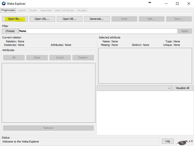
1. Run Weka. 2. Select Explorer from the Weka interface. 3. Open file (Fig. 1). Figure 1. Open file from Explorer in Weka. 4. Go to Select attributes. 5. Attribute evaluator WrapperSubsetEval (Fig. 26).
Figure 2. Select the attribute evaluator.
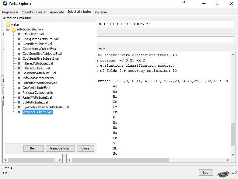
6. Left click (LC) on wrapper.
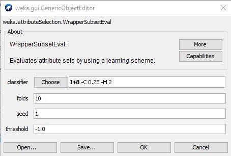
7. Classifier - select J48/Folds=10/Seed=1/Threshold= -1 (Fig 27).
Figure 3. Parameters of the wrapper.
2
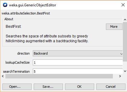
8. Search method- BestFirst/LC/direction: backwards, OK (Fig. 28).
Figure 4. Parameters of the BestFirst.
9. Use full training set. In a second pass, you can also try Cross validation 10. 10. Start.
This is a good but slow method. For the analyzed data set, Weka selected 18 elements of 35 as the most informative elements with a confidence of 92%, as shown in the line “Merit of best subset” (Fig. 5).
3
Faster Method
1. Open file.
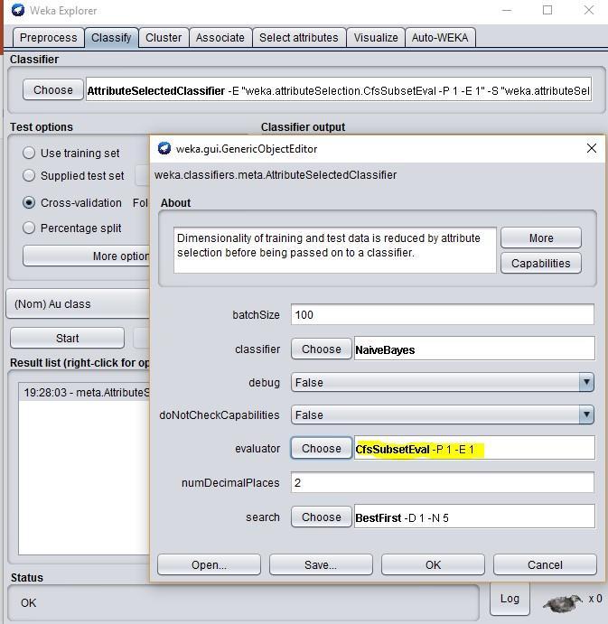
2. Classify/Meta/AttributeSelectedClassifier/ LC.

3. Classifier: NB (or J48).
4. Evaluator: CfsSubsetEval or wrapper/OK (Fig. 6).
4 Figure 5. The wrapper method selected the 16 most informative elements of the data set.
Figure 6.
method for
the most informative elements.
This method is fast and suggests the following elements as the best with a 92% of confidence: As, Bi, Cu, Ga, Ti. When using instead J48 as the classifier and the wrapper as the evaluator, Weka would suggest the same elements with a 92% accuracy but it will be much slower.
Even Faster Method
This method ranks each parameter in order to selects relevant elements, but it fails to detect redundant ones.
5
Faster
selecting
5. Start.
1. Open file. 2. Classify/Meta/AttributeselectedClaassifier/LC. 3. Classifier: NB.
4. Evaluate: GainRatioAttributeEval.
5. Search: Ranker.
6. The number to select: -1 will rank all elements, but you can specify the number of elements, e.g. 7 will rank the first seven elements.
Weka, with a confidence of 86.8% selected: Bi, Cu, Mn, Ag, As, S, Fe, and Ca as the most relevant. If you use the test set, Weka identifies the same elements but with a confidence of 93.1%.
You can also try other types of algorithms. Table 1 shows the results for the different types I tested.
Table 1. Results using different evaluators.
Relief and OneRAttribute Eval are less recommended.
6
Exploratory data analysis with Weka
7
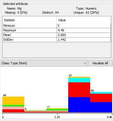
By opening a dataset, you can see the basic statistics on the right side of the panel (Fig. 7). Figure
7. Statistical parameters of an attribute.
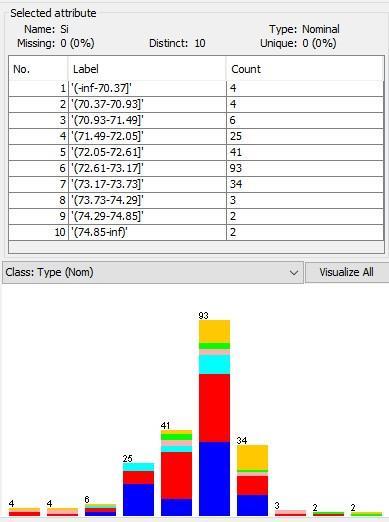
Histograms A more useful method is to see the histograms of each attribute. To obtain these histograms: 1. Open file. 2. Choose Filter/Unsupervised/Attribute/Discretize. 3. LC/ Set the number of bins between 10 15/OK/Apply (Fig. 8).
Figure 8. Histograms and bins for the selected attribute.
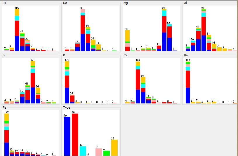
You can see all histograms at the same time by selecting Visualize All (Fig. 9).
Figure 9. All histograms of the studied dataset.
8
Some classifiers, like Naïve Bayes, work better with discretized data. For the rest, click on Undo after you obtained the histograms.
Removal of statistical outliers
1. Open file.
2. Filter/Unsupervised/Attribute/InterQuartileRange/Apply.
3. Filter/Unsupervised/Instance/RemoveWithValues/LC.
4. Nominal index last/OK/Apply.
5. Save your new table without outliers.
Clustering
Define number of clusters
EM also determines the number of clusters, and you can use the class if it is categorical, but it is slow.
1. Open file (reduced).
2. Cluster tab.
3. Select EM.
4. Select training set reduced/Close.
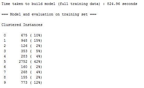
5. Start (Fig. 11).
Figure 10. Clusters determined by the EM method.
Clusters 5, 1, 9, and 0 are the most significant. So, we also obtained 4 clusters by this method.
9
Only two clusters
A useful technique to quickly explore your data is to force a cluster analysis with two groups. Accepting the concept that you have a mineralized zone in the limits of your license and that such mineralized zone will be different from the barren areas, a 2 component cluster should divide your data in a large group (barren) and a smaller group (potentially mineralized).
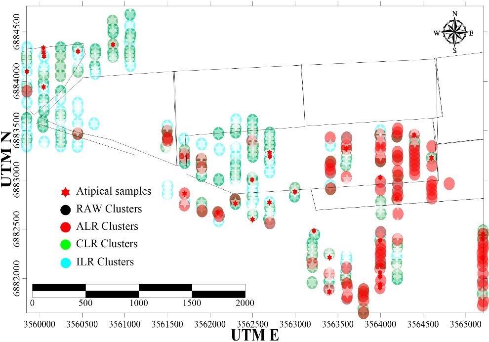
Plotting the coordinates of the smaller group on a map will give you an idea of the ore potential of your target (Fig. 12).
Figure 11. An example of the use of 2-component clusters to identify potential ore zones.
Based on these results, the Client arranged the limits of its claims to include the newly identified targets to the south of their current licenses.
To obtain the actual clusters, I recommend using this Excel macro (http://ow.ly/lopq30dBkkj) or CoDaPack.
10
Using the experimenter in Weka
While I believe that the Experimenter should be run as a first pass to test different classification models, I decided to explain the individual methods first. The Experimenter will tell you the general effectiveness of the different methods you want to test, so later you can do more detailed modeling in the Explorer mode.
11
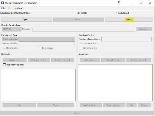
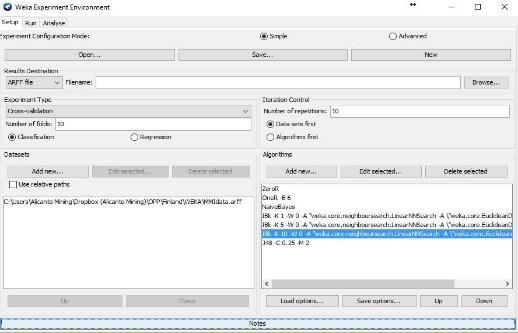
To use the Experimenter: 1. Run Weka. 2. Select the Experimenter. 3. Select New (Fig. 13). Figure 12. Select a new experiment option. 4. Left side add new folder. 5. Right side add new classifiers (Fig. 14).
Figure 13. The menu of the Weka Experiment Environment.
I suggest you test the following classifiers:
5a. ZeroR to establish the baseline. Any classifier must be higher than this value.
5b. OneR if you have a single classifier in your data, this will give you the best value.
5c. Naïve Bayes if the samples are truly independent and all are equal, Naïve Bayes will give you the best result.
5d. Lazy iBk Test for different K values (e.g. 1, 5, 10, etc). If all attributes are equal, this will give you the best result.
5e. J48 is the most efficient classifier and has the choice to create classification trees.
6. Go to the Run tab and click Start.
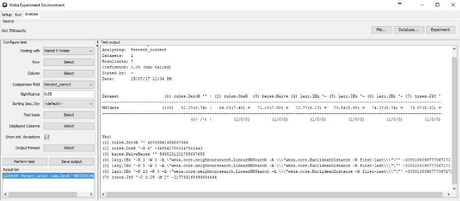
7. Go to the Analyze tab, click Experiment, click Show standard deviation and click Perform test (Fig. 15).
12
8.
Figure 14. Results of the different classifiers.
You can see that all the classifiers performed significantly better than ZeroR and OneR, so J48 is the recommended classifier.
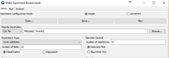
If you want to save the details of the experiment, go back to Setup and select a type of file, a name and a place where to save, click on the Run tab, and click on Start (Fig. 16).
13
Figure 15. Saving the results of your experiment.
14
