
PROEFMATERIAAL©VANIN
Chapter 1
The Unit Circle
PROEFMATERIAAL©VANIN
1.1 Purpose
The unit circle is a basic building block of trigonometry. The unit circle will be the starting point to explain the concepts of:
• angle: what is an angle and how can you measure an angle?
• sine, cosine and tangent of an angle
• The arc functions, which are the inverse of the sine, cosine, and tangent functions.
In this course, you will use the sine and cosine to create timed animations, lighting calculations, and transformations. Sine and cosine also play an important role when solving right triangles (a triangle where one of the internal angles is 90°). We end the chapter with the conversion between radians and degrees and vice versa, and the general formula to convert a value from one range to another.
1.2 The Unit Circle
In this first part of the chapter, you will explore all the concepts related to the unit circle. You will start by learning about angles in radians and degrees and understand how they connect to the unit circle.
A circle
The unit circle is defined a s the collection of points that are at unit distance from a central point ( M1 in the figure below). As you move the point P1 along the circumference of this unit circle, the distance between P1 and M1 is always exactly one unit, which is the definition of the radius of a circle.
-1 0 1 -1 1 1 1 Chapter 1 The Unit Circle 11
An arc on the unit circle
An arc is defined as a part of a curve, and more specifically a part of a circle. The following figure demonstrates an arc on the unit circle:
PROEFMATERIAAL©VANIN
Think of an arc as a flexible piece of string lying along the curve of the circle. If you straighten this string, its length can be measured. This length, when compared to the circle’s radius, is an important element when measuring angles.
A chord on the unit circle
A chord is defined as a segment that connects two points on the circumference of a circle. The following figure shows a few of examples of chords:
Chords that are horizontal or vertical will have a relationship with the sine and cosine functions we will see later on.
-1 0 1 -1 1
Chapter 1 The Unit Circle 12
1.3 Cartesian axis system
A two-dimensional (2D) axis system is used to locate points and vectors in space. Typically, the horizontal axis is called the X-axis, and the vertical axis is called the Y-axis.
A cartesisan axis system with the axises X and Y and two points.
PROEFMATERIAAL©VANIN
A point in 2D is written as (x y) and you can write the location of point A and B as follows:
• A = (3 1)
• B = (–2 –3)
Other examples are some points on the unit circle with the following coordinates:
• P1 = (1 0)
• P2 = (0 1)
• P 3 = (–1 0)
• P 4 = (0 –1)
You will use this notation extensively in the chapters about vectors and transformations.
-6 -5 -4-3 -2 -1 0 1 2 34 5 -6 -5 -4 -3 -2 -1 1 2 3 4 5 ⃗ ⃗
⃗ ⃗ 1 2 3 4
13 Chapter 1 The Unit Circle
1.4 Angles
An angle is formed by two lines that start at the same point, also called the vertex.
A segment is defined as the part of the line between two points that are on that line. The notation of a segment typically uses the names of these two points with a line on top, e.g. A1B1 is the segment from point A1 to B1
In the following figure, the two lines are the segments A1B1 and A1C1, and the vertex is the point A1.
PROEFMATERIAAL©VANIN
An angle is defined by how much you need to turn or rotate one segment around the vertex to align it with the other segment. In the figure that angle α equals 45.5°, which means that if you turn the segment A1B1 with A1 as centre of rotation over 45.5°, the segment A1B1 will be perfectly aligned with the segment A1C1.
1 1 1
Chapter 1 The Unit Circle 14
Most students learn to work with a protractor in high school, which allows them to measure angles in 2D figures. In the figure the angle β equals 36° which is the value you will also find when aligning the protractor with one of the two segments.
When developing games, however, you need to use mathematical tools to measure angles. For this calculation you first need the trigonometric formulas within a right triangle. As not all triangles are right triangles, it is also important to discuss the law of cosines. Finally, the concept of vectors will offer a generalised way to calculate angles with the dot product formula.
10 20 30 40 50 60 70 80 90 100 110 120 130 140 150 160 170 2 2 2
Chapter 1 The Unit Circle 15
PROEFMATERIAAL©VANIN
1.5 Angles - Icosahedron
An interesting shape is the icosahedron. This shape is used in Dungeons & Dragons games, which is a popular pastime for students and teachers alike. An icosahedron is made out of equilateral triangles (which are triangles where all the sides have equal length). The interior angles of such triangles are necessarily 60°. You can create an icosahedron by cutting out the following shape. Fold the dotted lines and glue the triangles together:
PROEFMATERIAAL©VANIN
The scientific term for an arrangement of triangles that can be folded into a 3D shape is a net After glueing everything together you should get the following icosahedron. If you use cardboard you could even use it as 20 sided die:
Chapter 1 The Unit Circle 16
This shape is used a lot in 3D editors such as Maya, Blender, 3 ds Max, Houdini, ... because it has nice properties with regards to rendering and texturing. There are also interesting mathematical questions to ask about this shape:
• If we construct this shape, will all the vertices (corner points) lie on a sphere ?
• Will this be a fair die? In other words, does every side have an equal chance to be thrown?
The answers to these questions will probably still be elusive for you right now. With the introduction of the concept of vectors we will revisit these problems.
1.6 The Unit Circle
Angles
Within the unit circle we can now define an angle α which is formed by the points M1, P1, and U x. Within the unit circle the point M1 will always be the vertex and the segments OP1 and OU x form the two lines that define the angle α.
U x is a reference point in the unit circle. This point is located on the X-axis and all the angles within a unit circle are relative to this point.
In the following figure the point P1 together with the reference point U x defines an angle α equal to 45°. Note that a positive angle indicates a counter clockwise direction.
PROEFMATERIAAL©VANIN
Another example is the angle β which is defined by the segments M1P2 and M1Ux and again the vertex M1. This angle is again defined in a counter clockwise direction and is equal to 113°
1 1
Chapter 1 The Unit Circle 17
PROEFMATERIAAL©VANIN
1.7 Unit Circle Quadrants
The unit circle can be divided into four quadrants, again number in counter clockwise fashion. Usually these quadrants are indicated with roman numerals.
The first quadrant (Q I) contains angles in the range of [0°, 90°].
The second quadrant (Q II) defines angles in the range of [90°, 180°].
The third quadrant (Q III) defines angles in the range of [180°, 270°].
The fourth and last quadrant (Q IV) defines angles in the range of [270°, 360°].
1 2
Chapter 1 The Unit Circle 18
1.8 Radians
So far all the angles were expressed in degrees, which is a unit that is easy to understand. You can also define angles in the radians unit which corresponds to the arclength on the unit circle. To illustrate what this means you can take a look at the following figure where we imagine what would happen if you straighten out a part of the unit circle. Try to predict or devine from the figure how long a piece of rope would need to be if you wrap it around the unit circle for a given angle.
Radians expressed with π
The figure now shows various multiples and parts of π on the Y-axis
The radians value is a physical value that corresponds to the length of the arc on the unit circle
The angle that is shown on the figure corresponds to 180° or π rad. The radians value of π or 3.14159 is also the length of a piece of string that you need to make half a circle with a radius of 1
-1.5 -1 -0.5 0 0.5 1 1.5 2 2.5 3 3.5 4 4.5 5 5.5 6 1 (a) = 0 -1.5 -1 -0.5 0 0.5 1 1.5 2 2.5 3 3.5 4 4.5 5 5.5 6 1 (b) = 40 -1.5 -1 -0.5 0 0.5 1 1.5 2 2.5 3 3.5 4 4.5 5 5.5 6 1 (c) = 80 -1.5 -1 -0.5 0 0.5 1 1.5 2 2.5 3 3.5 4 4.5 5 5.5 6 1 (d) = 120 -1.5 -1 -0.5 0 0.5 1 1.5 2 2.5 3 3.5 4 4.5 5 5.5 6 1 (e) = 160
-1/2 -1/4 0 1/4 1/2 3/4 5/4 3/2 7/4 1 1 (a) = 1 -1/2 -1/4 0 1/4 1/2 3/4 5/4 3/2 7/4 1 1 (b) = 21 -1/2 -1/4 0 1/4 1/2 3/4 5/4 3/2 7/4 1 1 (c) = 41 -1/2 -1/4 0 1/4 1/2 3/4 5/4 3/2 7/4 1 1 (d) = 61 -1/2 -1/4 0 1/4 1/2 3/4 5/4 3/2 7/4 1 1 (e) = 81 Chapter 1 The Unit Circle 19 PROEFMATERIAAL©VANIN
Radians as angle unit
A full rotation around the unit circle corresponds to an angle of 2π in radians
An angle α can be any value, even a negative one. For example, an angle with a value of 3π would be described as 2π + π and results in a angle of π.
Similarly, an angle of – π/3 corresponds to a positive angle of –5π/3. A negative angle on the unit circle means that the angle is defined in a clockwise direction. On the following figure you can see this negative angle.
PROEFMATERIAAL©VANIN
The maximum value of the angle in radians is 2π. The radians value corresponds to the arc length of the arc on the unit circle.
For a full circle, this arc corresponds to the circumference of the circle which is given by the following formula:
2π * radius
For the unit circle the radius equals 1.
This leads to a maximum value for the radians of 2π.
1
Chapter 1 The Unit Circle 20
1.9 Projection
A projection is a transformation which projects a point on another geometric object, typically a line. This projection is typically perpendicular, which means that the projection line needs to make an angle of 90° with the second line.
PROEFMATERIAAL©VANIN
In the figure, the point A will be projected onto the line which goes through L.
The point B is the projection of A onto the line.
Notice that the projection line is perpendicular to the line through L, and the angle is indeed:
90°
=
90∘
Chapter 1 The Unit Circle 21
α =
1.10 The Cosine Function
The cosine function is the first mathematical and trigonometric function that we discuss. You should understand what the process is to construct the cosine of an angle. The following sets of figures demonstrate this relationship.
We start with a point P1 which defines an angle α on the unit circle.
PROEFMATERIAAL©VANIN
The cosine of α is the value of the projection of the point P1 on the X-axis, in other words, a projection in the vertical direction on the X-axis. The cos(α) is now the signed length of this segment.
For an angle 0.785 in radians or 45°, the value of cos(α) = 0.707
= 45∘ 1 = 45∘ 1 = 45∘ 1
Chapter 1 The Unit Circle 22
1.11 The Sine Function
The sine of α is the value of the projection of the point P1 on the Y-axis, in other words, a projection in the horizontal direction.
We start again with a point P1 which defines an angle α on the unit circle.
PROEFMATERIAAL©VANIN
The sine of α is the value of the projection of the point P1 on the Y-axis, in other words, a projection in the horizontal direction on the Y-axis.
The sin(α) is now the signed length of this projection.
For an angle 0.7854 in radians or 45°, the value of sin(α) = 0.7071
= 45∘ 1 = 45∘ 1 = 45∘ 1
Chapter 1 The Unit Circle 23
1.12 Geometric Interpretation of the Tangent
The tangent of an angle is found by extending the segment OP to where it intersects with the tangent line. The tangent of an angle can be negative. The tangent of α is the result of the division of the sin(α) and cos(α) The formula to calculate the tangent therefore is:
PROEFMATERIAAL©VANIN
For an angle 0.7854 in radians or 45°, the value of tan(α) = 1
= 45∘ ′
=
.
Chapter 1 The Unit Circle 24
1.13 Tangent - Derivation
A first triangle has sides with lengths sin(α), cos(α) and 1, and an angle α.
PROEFMATERIAAL©VANIN
The second triangle has sides with lengths x, 1, and also an angle α
The two triangles are similar because they share the angle α, and both triangles have an angle of 90°. If two angles are the same, then by definition, the third angle is also the same.
1 1 1 1 1
Chapter 1 The Unit Circle 25
If two triangles are similar, the only differences between the triangles is the scale
PROEFMATERIAAL©VANIN
We can write:
1 1 1 1
1 = or: = =tan(
Chapter 1 The Unit Circle 26
)
1.14 Conversions as Interpolation
How to convert values from one unit to another
A common problem in computer graphics is the need to convert one unit of measurement to another unit of measurement. Examples are:
• Conversion from degrees to radians
• Conversion from radians to degrees
• Conversions from a color in the range of [0,1] to a range of [0,255]
The following figure shows you how to interpret this conversion graphically. The top segment has a range defined as [2, 3], while the bottom segment has a range defined as [0.5, 4].
PROEFMATERIAAL©VANIN
The problem is then to start with the value of s which is equal to 1.5 and project s on the second segment to calculate the value of d which will be 2.25
Example: Converting from radians to degrees
A typical application of this concept is the conversion between radians and degrees. The radians value is shown in the picture below. The range of an angle in radians is [0, 2π] and the range in degrees is [0°, 360°]. This makes the conversion process easier as both ranges start with 0.
-1 0 1 2 34 5 = 1.5 = 2.25
Chapter 1 The Unit Circle 27
The radians value shown above is converted to the degrees value in the picture below. We do this in two steps. First we divide the value in radians by the maximum value of the radians unit (which is 2π ):
PROEFMATERIAAL©VANIN
The next step is to multiply this t value with the maximum value of the degrees unit:
Remember that this process only works if both ranges have a minimum value of 0. You will discover the full formula for any conversion in the next sections.
Graphical interpretation
The t value can be understood as a normalized value in the range [0, 1].
-1/4 0 1/4 1/2 3/4 5/4 3/2 7/4 2 9/4 5/2 =
= 2 ∗ = 1.047 2 ∗ = 0.167
α = t*360° = 60° 0∘ 45∘ 90∘ 135∘ 180∘ 225∘ 270∘ 315∘ 360∘ 405∘ =60∘
0 1/4 1/2 3/4 5/4 3/2 7/4 2 =1 Chapter 1 The Unit Circle 28
The formula to calculate t is:
PROEFMATERIAAL©VANIN
From the t-value you can now calculate the new value in radians: αdeg = t *360° = 57°
When converting from one range to another you always convert the first range to a normalised range of [0, 1] and as a final step convert this range to the new desired range:
1. Check the range of the value you want to convert. [0,2π]
2. Convert this range to a range of [0,1]. In this case this means dividing by 2π.
3. Convert this new range to the desired range of [0,360°], which means you need to multiply by 360°.
Finally, you can combine this into one formula:
= 2 ∗ = 0.16 00.10.20.30.40.50.60.70.80.9 1 1.1
=0.16
0∘ 45∘ 90∘ 135∘ 180∘ 225∘ 270∘ 315∘ 360∘ 405∘ =57∘
= ∗ 360 2 ∗ = ∗ 180 Chapter 1 The Unit Circle 29
1.15 General conversion
A more general example is shown below. The values for the old range are: oldmin = 100 and oldmax = 300
The t value is 0.25 and the formula to calculate t is:
A value in this range is converted into a value in a new range with the following parameters: newmin = 50 and newmax = 100
The new value can then be calculated:
The radians value shown above is converted to the new range value in the picture below:
= = 0.25
result = newmin + t * ( newmax – newmin) = 62.5 result = newmin + 0.25 * ( newmax – newmin) = 62.5 Old range 50 100150200250300 350 = 150 New range
40 5060708090100 110 = 62.5 Chapter 1 The Unit Circle 30
PROEFMATERIAAL©VANIN
Chapter 2 Trigonometry
PROEFMATERIAAL©VANIN
Trigonometry deals with the calculation of angles and distances within triangles.
Most of the concepts are derived from the definitions of sine, cosine and tangent in the unit circle. It is, therefore, very important to see the link between the trigonometry concepts and the concepts of the unit circle.
We will start with the definition of a right triangle and continue with the relationship between any right triangle and a triangle within the unit circle.
2.1 Trigonometry
Given a right triangle defined by points A, B, and C. An important point to make is that you will label the sides as seen from point A. As visualised by the protractor, the angle at point C in this triangle equals 90°.
• hypotenuse: this is the longest side in a right triangle. The angles that are connected to this side are always smaller than 90°.
• opposite: this side is opposite to point A.
• adjacent: this side is adjacent to point A
A right triangle is defined as a triangle where one of the angles is 90°, as shown in the picture where the angle ɣ is 90°. The sum of angles in a triangle is always 180°.
△ 40 50 60 70 80 90 100 110 120 130 140 150 160 170 opposite hypotenuse adjacent △ opposite hypotenusa adjacent △
Chapter 2 Trigonometry 31
2.2 Sum of Angles
It is easy to claim that the sum of angles in any triangle is 180°. However, you can create visual proof of this statement:
The triangle shown here does not have a right angle.
PROEFMATERIAAL©VANIN
As a first step you extend the segment AC, because the trick is to try to move all the angles around point A
△ △
Chapter 2 Trigonometry 32
Next, you create a line parallel to segment BC and paste it onto point A Thus, you get a new segment B’A
PROEFMATERIAAL©VANIN
As a final step, we can find the angle β between the new angle ɣ and the original angle α. You can now see that the sum of these angles equals 180° .
△ ′ △ ′
Chapter 2 Trigonometry 33
2.3 Pythagoras
The Pythagorean formula in a right triangle is the well known formula:
PROEFMATERIAAL©VANIN
a 2 + b 2 = c 2
Where
• c is the hypotenuse or the longest side in a right triangle.
• a and b are the short sides of the triangle.
This formula is frequently used in game development to calculate distances between points and to calculate the length of a vector.
c b a △
Chapter 2 Trigonometry 34
2.4 Pythagoras Proof
Proof
There is a nice visual proof of the Pythagorean formula. You start again with a right triangle with sides a, b, and c
PROEFMATERIAAL©VANIN
The hypotenuse is c and the angle ɣ equals 90° .
You can now create a square where all the lengths are equal to a + b
As a next step you create four copies of this triangle. Because of the way the triangles are arranged there is an empty spot in the centre with an area of exactly c 2 .
a b c △ a b c △ a b c △ △ △ △ △
Chapter 2 Trigonometry 35
You can now rearrange two of the triangles and the segments above to show another way to calculate the empty area which is: a 2 + b 2
PROEFMATERIAAL©VANIN
Since you did not create an additional empty area, the two empty areas must be equal and you have now proven the Pythagorean formula: a 2 + b 2 = c 2
a b c △ △ △ △ △ a b c △ △ △ △ △
.
Chapter 2 Trigonometry 36
2.5 Right Triangle Formulas
To derive the formulas for a right triangle we take another look at the unit circle:
You start with a point P on the unit circle, which defines an angle on the unit circle. The segment c has a length of 1 because P is a point on the unit circle.
PROEFMATERIAAL©VANIN
Next you project downwards from point P to find the cosine of the angle α . This projection makes a right angle with the horizontal axis, visualised by angle ɣ
=
)
Chapter 2 Trigonometry 37
Next you project horizontally on the vertical axis to find the sine of the angle α
PROEFMATERIAAL©VANIN
Finally, you move this last segment to the right to create a triangle within the unit circle. Because the cosine and sine functions work with perpendicular projections, the lengths of side a and side b equals the cosine and sine of the angle α
In a right triangle where the hypotenuse has a length of 1 the sides of the triangle correspond to |cos (α)| and |sin(α)|. Within the unit circle it is easy to discern which one of the two sides is the cosine of the angle and which one is the sine of the angle. However, if the triangle is rotated, you need to carefully consider which side is the adjacent, and hence the cosine of the angle, and which side is opposite, and hence the sine of the angle.
= ) = ) △ = ) = )
Chapter 2 Trigonometry 38
2.6 Scaling up the Unit Circle
Compared to the unit circle in the previous section you can now apply a scaling transform on the triangle.
The scaling transform multiplies all the sides of the triangle with the same number. In game development this is typically referred to as a uniform scale. An important property of this transform is that the angles within the triangles will remain the same.
In the following figure the scale that you apply is the radius r which is equal to 3.
PROEFMATERIAAL©VANIN
=3
The segment c has a length of 3 because P is a point on a circle with radius = 3 The right triangle’s other two sides are also scaled up by a factor of r = 3 in this figure.
=3
3
)
)
Consider again that if you start from the centre of the circle in the figure, we can label the sides of the triangle as follows:
• a: adjacent side
• b: opposite side
• c: the hypotenuse. This side is also equal to the radius r in this circle.
In any right triangle we can then state:
△ =
=
=
=
= =
= ) = )
• a = c: cos (α) ⇒ cos (α) = • b = c: sin(α) ⇒ sin(α) = • = ) ) = ) ) = tan(α) Chapter 2 Trigonometry 39
2.7 Right Triangle Formulas
When confronted with a right triangle problem it is very important to label the sides of the triangle correctly. In the following figure we look at the problem from the perspective of point A. =hypotenuse = adjacent = opposite
You can use the following thought process to label the sides of the right triangle:
• Starting with the sides that are connected to point A the longest side will always be the hypotenuse or the segment c.
• The other side that is connected to point A can only be segment a or the adjacent side.
• Finally, the side that is not connected to point A must be segment b or the opposite side.
PROEFMATERIAAL©VANIN
The right triangle forααmulas for the sine, cosine and tangent of the angle α are:
) = ) = ) =
Chapter 2 Trigonometry 40
2.8 Polar Coordinates
An interesting application of sine and cosine is that they allow you to define a point with an angle and a radius.
PROEFMATERIAAL©VANIN
On the unit circle
The sine and cosine of an angle can now be used to calculate a 2D coordinate.
For an angle 0.7854 in radians or 45°, the value of P1 = (0.7071 0.7071).
1 1
Chapter 2 Trigonometry 41
1 1
You can calculate this point with the following formula:
P1 = (cos(α) sin(α)).
PROEFMATERIAAL©VANIN
With the actual value of α filled in, the formula is:
P1 = ( cos(0.7854) sin(0.7854) )
Note: in most programming languages the radians value is used for calculations, so you had better get used to this convention.
Chapter 2 Trigonometry 42
2.9 Breaking out of the Unit Circle
PROEFMATERIAAL©VANIN
Now we use the cosine and sine of an angle together with a radius to calculate a point on an arbitrary circle.
For an angle 1.0472 in radians or 60° , and a radius of 2.5, the value of P1 = (1.25 2.1651).
Polar
1 ) ) 1
coordinates
Chapter 2 Trigonometry 43
You can calculate this point with the following formula:
P1 = ( , {&yr} ).
PROEFMATERIAAL©VANIN
With the actual value of α filled in, the formula is:
P1 = (2.5 cos(1.0472), 2.5 sin(1.0472 ))
Note: in most programming languages the radians value is used for calculations, so you had better get used to this convention.
) ) 1 ) ) 1
Chapter 2 Trigonometry 44
2.10 Arc Sine
The inverse trigonometric formulas project a point from an axis back onto the circle. For the inverse sine formula (arcsin), a value is projected from the vertical axis.
PROEFMATERIAAL©VANIN
We start with a point A on the vertical axis. The y-position of point P has to lie within the unit circle on the vertical axis, which means that the maximum is 1 and the minimum is –1. The y -position is 0.5 in this example.
Point A is then projected to the right to find the intersection with the unit circle, resulting in the angle α1 with a value of 30° . Notice how this angle varies between 90° and –90°. There is still another way to project this point, do you know which?
If we can project to the right, we can also project to the left, resulting in the angle α 2 with a value of 150°
1 1 2
Chapter 2 Trigonometry 45
We can conclude that the formula arcsin( y) leads to two equally valid results, namely α1 and α 2. In this case: arcsin( y) = arcsin( y) = 30° or 150° .
PROEFMATERIAAL©VANIN
2.11 Arc Cosine
The inverse trigonometric formulas project a point from an axis back onto the circle. For the inverse cosine formula (arccos), a value is projected from the horizontal axis.
We start with a point B on the horizontal axis. The x-position of point P has to lie on the horizontal axis within the unit circle, which means that the maximum is 1 and the minimum is –1.
Point B is then projected upwards to find the intersection with the unit circle, giving the angle α1 with a value of 60°
Notice how this angle varies between 0° and 180°.
1 2
1
Chapter 2 Trigonometry 46
If we can project upwards, we can also project downwards, giving the angle α 2 with a value of – 60°
Notice how this angle is the negative value of α1.
PROEFMATERIAAL©VANIN
We can conclude that the formula arccos (x) leads to two equally valid results, namely α1 and α 2. In this case: arccos (x) = arccos (x) = 60° or – 60°
1 2 1 2
Chapter 2 Trigonometry 47
2.12 Arctangent
The arctangent is a frequently used function in game development, as it can be used to calculate an angle when you have a horizontal and a vertical distance. However, there is one important consideration: the formula is a ratio (division) of the two short sides of the triangle, with the adjacent side in the numerator: ) =
When the adjacent side is zero, the tan(α) is undefined and it is also not possible to calculate the arctangent
opposite
adjacent
You might wonder if a similar problem occurs for the sine and cosine functions. Indeed, there is, because the hypotenuse is in the numerator. This is only a problem if both the adjacent and opposite sides are equal to zero.
2.13 Inverse Formulas – Atan2
Most programming environments avoid the danger of the arctan function with a function called atan2 . This function is defined as follows:
α = atan2 (opposite, adjacent)
This function avoids the division and returns a correct value between –π and π or –180° and 180°.
Chapter 2 Trigonometry 48
PROEFMATERIAAL©VANIN
2.14 Non Right Triangles – Extra
The right triangle that we discussed so far is a special, because one of the angles in the triangle is 90°. You will encounter other triangles as well, so it is important to showcase how to solve acute or obtuse triangles.
PROEFMATERIAAL©VANIN
We start with an acute triangle defined by points A, B, and C, which are given. All of the angles in this triangle are smaller than 90° .
We divide the triangle into two right triangles by projecting point C on the horizontal axis, resulting in point D.
Chapter 2 Trigonometry 49
This results in two right triangles △ AC D and △ BC D, with a side h whose height is still unknown
PROEFMATERIAAL©VANIN
You can work out the solution by trying to find a formula for x . As a first step we write down the Pythagorean formula for both triangles:
△ ∶ 2 + ℎ2 = 2
△ ∶ ( )2 + ℎ2 = 2
Because h is unknown we try to get rid of this variable:
∶ ℎ2 = 2 2
Combining both formulas gives the following equation:
c 2 – x2 = b 2 – a 2 + 2 a x – x2
Both sides have –x2 so we can simplify to:
c 2 = b 2 – a 2 + 2 a x
Now we can isolate x because a, b and c are known: = 2 2 + 2 2
△ △ ℎ
△
△
∶ ℎ2 = 2 ( )2 = 2 2 + 2 2
Chapter 2 Trigonometry 50
Chapter 3 Introduction
PROEFMATERIAAL©VANIN
3.1 Animation
The trigonometric functions and formulas allow you to calculate angles, position points via polar coordinates, and solve trigonometric problems.
The sine and cosine functions can also be used to create simple animations which is the major topic for this chapter.
The chapter starts with an explanation of the concept of timeline and frame based animation. In games and 3D editors time is an important aspect of the development of animation and game play. Sometimes an absolute time is used, in other instances the time difference or delta time between two frames is sufficient to programme an animation.
The concept of using functions to control animations is the next topic, and the sine and cosine functions are used here to demonstrate how to control the timing with the help of mathematical functions.
3.2 Timeline
Games, animations and films are the digital world. As such it is common to hear concepts as frames per second (fps) or framerate. The framerate of a film or game is linked to the mathematical concepts of frequency and period which you will discover later on in this chapter.
For gamers the fps is an important metric when judging the quality of a game, i.e. a possible a potential for an fps drop can be detrimental to the fun of a game. For smooth motion and responsiveness the fps should strive to match the framerate of the monitor. Most game companies aim for at least 30 frames per second for games, while 60 frames per second is considered good. With the advent of modern monitors, the framerate for games can be even higher, for example 90 or even 144 frames per second. Although a high framerate is preferred in games it is also important to synchronise the frames to the framerate of the monitor. A typical problem is tearing where the lack of synchronisation results in a visible tear in the image.
For virtual reality applictions this is even more important as low framerates in these cases can induce dizzyness or even nausea. In cinematic settings a framerate of 24 frames per second is the gold standard. Most animation tools such as Houdini, Blender or Maya will use this setting as the default when you create character animations or film clips. The historical reasons for this framerate are varied. At the start of the film industry there was no generally accepted standard for film framerates, the only consensus was to keep the framerate low to reduce costs, which resulted in a framerate of about 16 frames per second. Cameras were handcranked, so this framerate was only by approximation.
There are different reasons for switching to 24 fps. The most important reason is that this framerate is an important threshold for visual perception. At 24 fps, a film appears to have continuous motion for most people. Another reason for the change is the introduction of
Chapter 3 Introduction 51
audio to films which necessitated a better framerate. Finally, for some the reason was mathematical as 24 has six dividers: 2,3,4,8,6,12. Whatever the reason, 24 fps is what people expect when they go see a film. Some films experiment with this setting, for example, “The Hobbit” was filmed at 48 fps. However, this was a change that was not received well by critics and audiences. Human perception remains subjective, so even though a framerate could be objectively better, people resist change. The following figure shows a time between 0 and 2 seconds with a framerate of 24 fps. Within this timeframe, 48 frames will be needed to create a cinematic animation.
PROEFMATERIAAL©VANIN
You can also calculate how much time passes between two subsequent frames. So if you have a timeframe of 2s and 48 frames the time between each frame can be calculated as:
The symbol Δt is commonly used to indicate a delta time, meaning a difference between two distinct moments in time.
3.3 Animation
If you want to create an animation, one of the important components will be the factor time. In a game or animation the time is the independent variable that dictates changes in an object’s position, rotation, and scale. If you want to animate a ball bouncing up and down, you need to calculate a new position for the ball for each frame.
0 2
= 48 =
Time Chapter 3 Introduction 52
In this chapter we will focus on using the sine and cosine functions to generate a new position. As the output of sine and cosine functions is limited to the range of [–1 1] it is necessary to add extra parameters if we want to achieve a specific movement.
PROEFMATERIAAL©VANIN
Time Sine parameters
A typical example is the motion of a platform in a game. The moving platform in the figure needs to move horizontally between the two points L and R
You can use the sine function for such a horizontal motion, and as you will see the sine function generates a simple but plausible animation for this moving platform. The first parameter of the sine function that will help achieve the desired result is the amplitude parameter, which allows you to modify the output range of the sine function.
The second parameter is the offset, that can move the centre of the sine function to the centre of the moving platform.
A third parameter is the frequency, which covers the speed of the moving platform animation. If you want the platform to move fast, a high frequency parameter will be required.
Finally, there is also a phase parameter, that allows you to change the starting position of the moving platform.
These four parameters and their influence on the shape of the sine function will be discussed in the following section.
Chapter 3 Introduction 53
3.4 The Sine Function
Sine function plot
We already covered the sine function in previous chapters. This week we discuss the sine function and plot out the relationship between the angle α and the sin(α) value.
Point P1 is traced along the circumference of the unit circle while the plot shows the value of angle α on the horizontal axis and the value of sin(α) on the vertical axis.
Notice some important characteristics of this shape. The maximum of the sine function is 1 and the minimum value is –1. The amplitude of the sine function is defined as the difference between the maximum and the minimum value, divided by 2. The amplitude is denoted with the letter a:
The sine function crosses the horizontal axis at α = π. Other important points are:
-2 -1 0 1 2 3 4 5 -1 1 1
= 2 = 1
⎧ ⎪ ⎪ ⎪ ⎨ ⎪ ⎪ ⎪ ⎩ ⇒ ( ) 0 ⇒ 0 3 ⇒ 1 ⇒ 0 3 2 ⇒−1 2 ⇒ 0 Chapter 3 Introduction 54 PROEFMATERIAAL©VANIN
3.5 Sine function shape
For clarity, we show the same sine function again, but now the horizontal axis shows a division that is based on multiples of π.
For an unmodified sine function, one full period takes 2π, and then the same shape is repeated again.
3.6 Parameters
The sine function is very interesting on its own, but you need extra parameters to make the sine function useful. The following parameters can be used:
• Amplitude – a: A sine function variates between –1 and 1, with the amplitude we can increase this minimum and maximum value.
• Frequency – f: One period has a duration of 2π, this can be changed with the pulsation parameter.
• Phase shift – Φ: This parameter can shift the sine function left and right (horizontal direction).
• Vertical shift – v: The vertical shift parameter shifts the centre of the sine function.
3.7 Sine function shape
The sine function without parameters has a minimum of –1 and a maximum of +1. One period of the sine function starts at 0 and ends at 2 π
-1/2 0 1/2 3/2 2 -1 1 1
-1/2 0 1/2 3/2 2
Chapter 3 Introduction 55
-1 1
PROEFMATERIAAL©VANIN
3.8 Amplitude parameter
The amplitude parameter determines the difference between the maximum and the minimum of the sine function. To implement this parameter you multiply the sine function with the parameter called a, which gives the following equation: a sin(t).
The amplitude a equals half the vertical distance from the maximum to the minimum of the sine function. This is visually represented by the distance 2a in the figure above. One way to determine the amplitude given the shape of the sine function is to divide this distance from top to top and divide by 2. An example of this calculation is as follows: = ( ) 2 = (1.5 −1.5) 2 = 1.5
As an exercise, take a look at the following figure:
Use the given formula to determine the amplitude of this sine function.
-1/2 0 1/2 3/2 2 -3 -2 -1 1 2 3 2
-1/2 0 1/2 3/2 2 -3 -2.5 -2 -1.5 -1 -0.5 0.5 1 1.5 2 2.5 3 2
Chapter 3 Introduction 56
PROEFMATERIAAL©VANIN
3.9 Frequency parameter
The frequency parameter determines how many periods there are within a range of [0s 1s] or one second. A period is defined as one full cycle of the sine function, which you can measure as the horizontal distance from top to top of the sine function. The unit of frequency is called Hertz and is abbreviated as Hz . The following figure demonstrates what a frequency of 1Hz looks like:
PROEFMATERIAAL©VANIN
There are three possibilities for this parameter:
• Frequency > 1Hz: There will be more than one period within one second.
• Frequency == 1Hz: There is exactly one period in one second.
• Frequency < 1Hz: There will be only part of a period within one second.
The formula for the sine function with only the frequency parameter is:
sin ( 2π f t )
Frequency > 1Hz
The following figure shows the result of a frequency of 2 Hz. Notice that there are more periods per second, and that by doubling the frequency the period has been halved.
The relationship between period and frequency is inverse. If the frequency increases by a factor of two, the period will decrease by a factor of two.
-2 -1 0 1 2 34 5 6 -2 -1 1 2 3 period= (2 )
-2 -1 0 1 2 34 5 6 -2 -1 1 2 3 period= (2 )
Chapter
57
3 Introduction
Frequency < 1Hz
The following figure shows the result of a frequency of 0.5Hz. Notice that there are less periods per second, and that by halving the frequency the period has been doubled
PROEFMATERIAAL©VANIN
3.10 Phase parameter Φ
The phase shift parameter determines a horizontal shift of the sine function. For a positive value of this parameter Φ, the sine function will be shifted to the left by an amount of Φ. In the figure below the value for Φ has been set to 1/3 π.
The original sine function with Φ set to zero sin(t) and the phase shift sine function with Φ set to 1/3 π which is + 3
The formula with only the Φ parameter is:
sin ( t + Φ )
The parameter Φ can be used to change the starting point of an animation. Without the phase, an animated object would by default always start at its centre position. The phase parameter allows you to pick a starting point anywhere within the range of motion of said object.
A positive Φ value will shift the sine function to the left
A negative Φ value will shift the sine function to the right.
-2 -1 0 1 2 34 5 6 -2 -1 1 2 3 period= (2 )
-1 0 1 2 =
Chapter 3 Introduction 58
3.11 Vertical shift parameter
The shift parameter generates a shift of the sine function in a direction perpendicular to its baseline (in this figure the horizontal axis).
Two examples of adding a shift parameter to the sine function with v1 = 1.5, and v2 = –2. The central line of the sine function is defined as the line that runs exactly through the centre of the sine function.
The shift parameter is added to the sine function as: = ( )+ 1
As pictured here, the output of the sine function is a coordinate y. In a 2D or 3D world you can use the output of the function and connect it to whatever variable you want. For example the sine function could modify the x or z-coordinate of an object.
3.12 Sine function shape
Finally, you can combine all the parameters for the sine function in one formula:
With the actual values for these parameters, the formula is:
-1/2 0 1/2 3/2 2 -3 -2 -1 1 2 1 = 1.5 2 = −2 baseline baseline t y
a 1 sin ( 2 πf 1t + Φ 1 ) + v1
0.5 sin ( 2 π2 t + 1/3 π ) + 2 Chapter 3 Introduction 59
PROEFMATERIAAL©VANIN
The period, amplitude and shift are relatively easy to read from this function plot. Period and frequency have an inverse relationship, which is given by:
PROEFMATERIAAL©VANIN
The phase Φ1 involves more work as it involves the useage of the arc sine and knowledge about the locations of the peaks or zero crossings of the function. The methodology to determine this parameter correctly will be discussed in the following section.
Application
You can already put the knowledge of the sine function into action. In the following figure we take another look at the platform problem from the beginning of the chapter. Remember that you wanted to make the platform move from left to right with a repeating cycle and a certain speed.
The first problem is that the platform has a width that you need to take into account and also a point P that is defined as the model centre of the platform. The first step you need to take is to think about the valid locations of this point P in this situation. P cannot be at the location L or R because then half of the platform would intersect with the boundaries of the world. The answer is then to restrict P to make sure it keeps a distance of half the width of the platform itself or 2 away from the boundary points L and R
By labeling the baseline and the amplitude we can determine the parameters a and v if the position of L and R are known.
-1/2 0 1/2 3/2 -0.5 0.5 1 1.5 2 2.5 3 3.5 4 1 1 = 2 period= t y
1
1 1
=
Chapter 3 Introduction 60
The x-coordinate of point L equals 1 and the x-coordinate of point R equals 6. Here you see the advantage of using the centre of the platform as model centre, because you can calculate the x-position of the baseline as the average between these two coordinates, which also corresponds to the parameter v:
PROEFMATERIAAL©VANIN
For the amplitude parameter you can calculate the distance of the left boundary to the baseline, which is calculated as the horizontal distance between the baseline and the left boundary:
3.13 Phase Control
By determining a and v you can already setup a sine function that will animate the platform within the defined boundaries:
= asin ( t ) + v = 2sin ( t ) + 3,5
Notice how the time t is used as argument in the sine function. The result of the sine function is then used as the x-coordinate for the point P. The clear message here is that you are free to use the output of the sine function wherever you want. The result might be stored in the x, y or z-coordinate of a point, but it is also possible to use the sine function to animate colours.
0 1 2 3 4 5 6 7 = 1 = 0.5 + = 1.5 baseline ! ! = 12 = 62 x
=
2 =
(1 + 6)
3.5
a = v – ( L x + w H ) = 3.5 – 1.5 = 2
x
Chapter 3 Introduction 61
The next problem you need to tackle is the starting position of the platform. You can first determine what the starting position would be of the platform at t = 0s:
PROEFMATERIAAL©VANIN
This corresponds to the x-position of the baseline and this indicates that at the start time of the game or simulation, the platform will be at the baseline position or the centre. It is possible to use the phase shift Φ to change this starting position. A common demand is for example to set the start position on the left boundary. This requires that at t = 0s, the point P must have the x-coordinate of : x = L x + wH = 1 + 0.5 = 1.5. You can now determine the phase by requiring that the sine function with an unknown phase must be equal to this coordinate x = 1.5 at time t = 0s:
The determination of the phase Φ will always involve setting a condition for the position of the animated object at a given time (usually at t = 0s). Determing the phase always involves an arc function. With the determination of Φ, the function is now:
When the condition is set at t = 0s, the frequency or period of the sine wave does not matter because the term in t will be zero. However, when the condition is set at a different time it will be necessary to take this frequency or period into account.
0 1 2 3 4 5 6 7 baseline ! ! = 62 x = 1.52
x
= asin ( t ) + v = asin ( 0 ) + v = 0 + 3.5 = 3.5
= ( + ) + ⇒ (0 + ) + 3.5 = 1.5 ⇒ 2 ( ) = 1.5 3.5 ⇒ ( ) = 1.5 3.5 2 ⇒ ( ) = 1 ⇒ = ( 1) = 3 2 1 2
= ( + ) + ⇒ 2
3 2 + 3.5
+
Chapter 3 Introduction 62
3.14 Cosine
The cosine function has similar characteristics to the sine function, but has been shifted over the horizontal axis.
The following picture shows the plot of the regular cosine function:
= cos ( α )
The cosine function starts with an initial value of 1. However if a bigger range of this function would be plotted, the function would look exactly the same as the sine function.
Sine and cosine are the result of the same operation, the only difference is that sine is projected on the vertical axis and cosine is projected on the horizontal axis. Therefore, the phase shift 2 , which is the result of the fact that the angle between these two axes is also 90° or 2 apart.
y
-1/2 0
3/2 2 y
1/2
-1/2 0 1/2 3/2 2 y 2
Chapter 3 Introduction 63
PROEFMATERIAAL©VANIN
3.15 Determining the Frequency
Control the timing of the sine function
PROEFMATERIAAL©VANIN
The period is the length of one full cycle of a sine wave and is typically expressed in the time unit seconds
The frequency is the number of full cycles per second
There is an inverse relationship between frequency and period: = 1 ⇒ = 1
When you want to control the timing of the sine function you need to express the timing either by frequency or by period. Hence, using the inverse relationship you can express the sine function in two ways: = (2 ) ⇒ = 2
For example, if f = 2Hz, then = 1 = 1 2 = , and both forms of the sine function (either with frequency or with period) would lead to the same sine function shape: = (2 2 ) = (4 ) = 2 0,5 = (4 )
The use of the period T in the sine function can be more practical than using the expression with frequency. It is sometimes easier to express how long the animation should take in seconds than to try and come up with a plausible frequency.
As an example, suppose we want the moving platform to complete one full cycle in 16s, and we call this period T 2. The frequency in this case would be f 2 = 1 2 = 0.0625Hz. When the period is bigger than 1s it seems to be easier to express the timing with the period instead of the frequency, and the expression for the sine function is also easier to read and understand: = 2 2 = 2 16 ⇒ 2 =
However, when the period is less than one second, it may be more practical to think in terms of frequency, particularly in scenarios where rapid oscillations are involved, such as in audio signals. Another example might be animations in games, such as those in the Steampunk genre, which feature rapidly rotating gears, wheels, ... with frequencies that are higher than 1Hz.
Chapter 3 Introduction 64
3.16 Period of Ordinary Sine
Why is factor 2π necessary?
The formulas for the sine function with frequency or period parameter were introduced without an explanation for factor 2π. For a better understanding of this factor we take a step back and revisit the sine function without parameters:
y = sin ( t )
You can make a table of important points of this sine function and calculate the values for t and y:
PROEFMATERIAAL©VANIN
The sin function in this case works with radians, and the period of the sine function without parameters is T = 2π = 6.2832s. The standard period of 2 π is cumbersome in practice, which is one reason why the factor 2π is included in the sine function. The frequency 2 = 0.1592Hz of the standard sine function is also impractical to work with.
In the next section you can further explore what the exact reason behind the factor 2π is. To understand this properly you need to rethink the section about conversions from one unit to another. This problem is similar in that we want to have a full cycle of the sine function in a period from 0s to 1s.
⇒ ( ) ⇒ 0 ⇒ 0 ⇒ 1 2 ⇒ 1 ⇒ 2 ⇒ 0 ⇒ 3 3 2 ⇒−1 ⇒ 4 2 ⇒ 0 ⇒ 5
0s 1s 2s3s 4s 5s 6s 7s -1 s 0 s 1 s t y 1 2 3 4 5
Chapter 3 Introduction 65
3.17 Sine function shape
Given the sine function:
PROEFMATERIAAL©VANIN
y = sin ( 2 πt )
You can now repeat the same process, but the range of t will be between 0s to 1s. Notice how this range between 0s and 1s in the first column is converted into a range of 0 to 2π radians in the second column. This effectively matches a period of 1s to a full cycle of the sine wave.
The figure shows that the effective period T of the sine wave is now 1s and the frequency = 1 = 1 = .
This formula results in a frequency of one Hz. How can we now control the frequencies of the sine wave?
⇒ 2 ⇒ (2 ) ⇒ 0 ⇒ 0 ⇒ 0 ⇒ 1 0.25 ⇒ 2 ⇒ 1 ⇒ 2 0.5 ⇒ ⇒ 0 ⇒ 3 0.75 ⇒ 3 2 ⇒−1 ⇒ 4 1 ⇒ 2 ⇒ 0 ⇒ 5
0 1 2 3 4 -1 1 t y = 1 2 3 4 5
Chapter 3 Introduction 66
3.18 Sine function shape
The final step in controlling the frequency or period of the sine function is to add the factor f or frequency in the formula or the alternative version with the parameter T. = 2 = (2 )
If you set the frequency f = 2, then the period = 1 = 1 2 = .
The function with the value of the frequency is:
You can now repeat the same process, but the range of t will be between 0s to 0.5s. Notice how this range between 0s to 0.5s in the first column is converted into a range of 0 to 2πradians in the second column. This effectively matches a period of 0.5s to a full cycle of the sine wave.
y = sin ( 2π 2Hz t ) = sin4πt
⇒ 4 ⇒ (4 ) ⇒ 0 ⇒ 0 ⇒ 0 ⇒ 1 0.125 ⇒ 1 2 ⇒ 1 ⇒ 2 0.25 ⇒ ⇒ 0 ⇒ 3 0.375 ⇒ 3 2 ⇒−1 ⇒ 4 0,5 ⇒ 2 ⇒ 0 ⇒ 5 0s 1s 2s 3s -1 1 t y = 1 2 3 4 5 Chapter 3 Introduction 67
PROEFMATERIAAL©VANIN
3.19 Applications – Extra
Animation
The exponential function is given as:
PROEFMATERIAAL©VANIN
This is a power function with e as its base, which is also called Euler’s number and this is a constant with a value of 2.71828
The exponential function decreases over time and reaches zero at +infinity. This makes it a good fit for animations that have to fade out over time. The λ value controls how fast the value of this function reaches zero. A value smaller than 1 for λ results in a slowly decaying function.
When the value of λ is bigger than 1, the function reaches 0 faster. The function below the orginal function has λ = 3 and almost reaches zero after 2 seconds. The function with the actual value for λ is then:
= e –3 t
y = e – λt
0
4 5 1 t y
1 2 3
0 1 2 3 4 5 1 t y
Chapter 3 Introduction 68
y
3.20 Applications – Extra
Animation
Previously, you used a constant (unchanging) amplitude for the sine function. However, you can use the previous section’s exponential function as slowly decaying amplitude and multiply it by the sine function to achieve a slowly decaying sine function. One example of where you can use this is a pendulum that slowly loses energy and stops swinging. The function is given by: e-λt sin ( 2 π f t )
If you set the value for λ to 1 and the value for f to 1Hz you get the following graph. The sine function is still detectable for the first 4 seconds, where you can see that the period T = 1s:
PROEFMATERIAAL©VANIN
3.21 Angular Velocity
You can now combine your knowledge about sine and cosine to create a variety of motion. The following figure illustrates what the possibilities are.
• Point P1 is defined as: ( cos ( t ) sin ( t ) ). This corresponds to a polar coordinate where the time t is used as angle for the cosine and sine functions. This coordinate moves along the unit circle over time.
• Point P2 is defined as: ( P2x sin ( t ) ). The x-coordinate of this point is constant, which results in a point that moves vertically.
• Point P 3 is defined as: ( cos ( t ) P 3y ). The y-coordinate of this point is constant, which results in a point that moves horizontally.
If we use time as input angle for the animation we can control the speed of this animation.
0
-1
1 2 3 4 5 6
1
2
1
3
Chapter 3 Introduction 69
3.22 Frequency
The formula for point P1 is:
PROEFMATERIAAL©VANIN
1 = (2 ) (2 )
With the value for the frequency given as: 0.25Hz, the actual formula for point P1 is now:
1 = (2 0.25 ) (2 0.25 )
The other two points are animated with the same frequency and are now:
• Point P1 is defined as: (P 2x sin ( 2 π f t ) ). The x-coordinate of this point is constant, which results in a point that moves vertically and with the frequency f = 0.25Hz.
• Point P 3 is defined as: ( cos ( 2 π f t ) P 3y ). The y-coordinate of this point is constant, which results in a point that moves horizontally and with the frequency f = 0.25Hz.
3
Chapter 3 Introduction 70
1 2
Chapter 4 Vectors
PROEFMATERIAAL©VANIN
Vectors are an important concept for creating games and animations. Vectors offer a framework where typical game development problems can be formulated in a mathematically sound but compact manner. The topics of this chapter include the following:
• Vectors versus points: In a game engine or 3D editor there is a difference between vectors and points. In this chapter this difference will be explained qualitatively, but as you will discover in the chapter about transformations, there is also a mathematically proper way to model vectors and points in the form of homogeneous coordinates. In general, points represent a location and time in space. Vectors on the other hand indicate a direction or movement of an object.
• Add and subtract points and vectors: Mathematical operations of adding points and vectors are important in the game world. For example, the remainder of two points results in a direction vector from the second point to the first point. The addition of two vectors can represent the combination of two forces acting upon an object.
• Length of a vector: When you use vectors to describe velocity, the length of this vector can be interpreted as the speed of the object. Another example is the calculation of the distance between two points, resulting in a vector with a length equal to the distance between the two points.
• Normalize a vector: It is sometimes necessary to modify the length of a vector. In such cases, reducing the vector to a length of 1 (defining it as a unit vector) is convenient. A normalized vector can then be thought of as representing only the direction of an object, which allows for precise control of the speed. Another use case for normalized vectors is the topic of lighting (or shading) where normalized vectors are required to correctly calculate the various elements of the lighting equation.
• Scale a vector: To implemenent movement you will model the velocity of an object with a vector. It is possible to decouple speed and direction with vectors to enable the control of these two elements.
• Coordinate systems: Vectors are used to describe coordinate systems, where for example a rotated coordinate system can be made by specifying rotated unit vectors.
A good understanding of the basic operations of vectors is necessary to further explore the concepts of the dot and cross product, which will be discussed in the following chapter. These two operations on vectors are crucial for implementing lighting, solving geometric problems and more advanced algorithms such as inverse kinematics. Vectors are also crucial in physics implementations within games or simulations, e.g. for object collisions or particle animations.
Chapter 4 Vectors 71
4.1 Vector
Definition
PROEFMATERIAAL©VANIN
A vector of dimension n is an ordered collection of n elements, which are called components:
• a 1D vector is typically referred to as a scalar or number
• a 2D vector is a vector of dimension 2 with 2 components, typically called x and y. Other names are possible, such as u and v for texture coordinates.
• a 3D vector is a vector of dimension 3 with 3 components, typically called x , y and z. Other names are for example r, g and b.
Notation
A vector is typically presented as a row of values in a specific order. A notation for a 2D vector where x equals 10 and y equals 5 is for example:
v 1 = (10 5)
For a 3D vector the same notation is used:
v 2 = (10 5 3)
Note: The names for vectors are typically lower case with a small arrow on top to indicate that this is indeed a vector.
It is useful to also have a way to name the components of a vector separately. The common way to do this is to add a subscript to the name of the vector, indicating the specific component. In a 2D example this can only be an x or a y-component:
v1x = 10
v1y = 5
The components of a vector are scalars (numbers), so it is not necessary to add an arrow on top of these components.
Vector in column format
Sometimes a vector is written as a column vector. This is the same concept, only with another notation.
The column notation for a 2D vector where x equals 10 and y equals 5 is for example:
⃗ 1 = 10 5
Chapter 4 Vectors 72
For a 3D vector the same notation is used, with the addition of a z-component that equals 3:
PROEFMATERIAAL©VANIN
The column format is typically used for matrix multiplications where a vector can be transformed (rotated or scaled) by multiplying with another matrix.
Graphical notation
A vector is drawn as an arrow to indicate its role in determining the direction. The start of the vector is also called the tail and the end of the vector is called the head
The components of a 2D vector indicate the horizontal and vertical difference between the tail and the head of the vector.
4.2 Vectors versus Points
Points
Points are used to define locations in a two dimensional or three dimensional space. Examples of the usage of points:
• Quest location: In games, quests can have important locations attached to them. One example is the location where a quest starts, or where a player can interact with a non player character (NPC), to start a quest.
• Particle location: The particle location is where a particle is currently visible.
• Vertex: A point inside a mesh is typically called a vertex
⃗ 2 = 10 5 3
= 10 =
head tail ⃗ 1
5
Chapter 4 Vectors 73
For points, the first coordinate describes the horizontal distance in a two dimensional cartesian axis system, while the second coordinate describes the vertical distance. Note also how the axis system is orthogonal, which means that the X and Y axis are 90° apart.
PROEFMATERIAAL©VANIN
Vectors
A vector is used to indicate a direction in two dimensional or three dimensional space. Examples for the usage of vectors:
• The direction a guard NPC is walking.
• The direction of a photon.
• The current direction of a particle. For example, for a smoke particle this could be an upwards direction.
In the figure two vectors, both called v are visualized. You should realise that a vector does not have a location, and drawing a vector at a certain location in a graph does not have a mathematical meaning. Drawing a vector at a certain location is purely for illustrative purposes; it is the direction of the vector and its length that carry the true meaning.
In this case, the vector v could describe the direction in which a guard at point G is moving.
x =
y = 6 X Y 1 = 5 6 2 2 3
5
x
y =
X Y ⃗ = 2 3 ⃗ 2 3 Chapter 4 Vectors 74
= 2
3
4.3 Example
The cars in the following figure show the concept of using points and vectors to model the behaviour of an object. The two cars on the right have the same direction vector:
1 = (–0.68 1.88)
PROEFMATERIAAL©VANIN
This is an important concept as it does not matter where a vector is displayed on a figure. It is just a matter of convenience to convey that v 1 is the direction vector of the first car, and v 2 is the direction vector of the second car.
The vector v 3 is different from the first two vectors as its components are different from the first two vectors:
The points P 1, P 2 and P 3 define the current locations of the three cars. In games and animations you give every object its own unique location.
v
v
2 = (– 0.68 1.88)
v 3 = (–1.73 1) ⃗ 1 1 ⃗ 2 2 3 ⃗ 3
Chapter 4 Vectors 75
4.4 Length of a Vector
The length of a vector is also called the magnitude, and is defined as the distance from tail to head of the vector. Calculating the magnitude of a vector is an operation that will be used to normalize vectors, to determine a distance between two points, or to calculate the speed at which an object is travelling.
PROEFMATERIAAL©VANIN
⃗ = 4 3 y = 3 = opposite x = 4 = adjacent
The length of a vector is an application of the pythagorean formula in a right triangle: 2 + 2 = 2 ⇒ = 2 + 2
As always, you need to correctly identify the sides of the triangle to apply the formula.
= 4 3
The cartesian grid is orthonormal, which means that there is an angle ɣ equal to 90°. The length of a vector is written symbolically with two vertical lines around the vector: |v |.
It is no coincidence that the same symbol is used for the absolute value of a scalar, because you can interpret a scalar as a one-dimensional vector. Thus, the absolute value of such a vector is its length. y = 3 = opposite
= 4 3
= 4 = adjacent | ⃗|=
The length of the vector is given as: | ⃗ | = = 2 + 2 = 42 + 32 = √25 = 5
X
|
Y ⃗
Y
⃗|= X
Y
x
X
⃗
Chapter 4 Vectors 76
Examples
The components of the three vectors are given by:
To calculate the lengths you apply the pythagorean formula:
A common error in vector calculations is incorrectly squaring the components when determining a vector’s magnitude. Remember that each component’s square contributes positively to the total magnitude, regardless of whether the original component is negative: ( 1)2 = 1
When you calculate the magnitude of a vector, you are taking the square of the components of a vector. These components can be negative but the square of them should be positive. Neglecting to square the components correctly will result in an inaccurate magnitude.
⃗ 1 ⃗
⃗
2
3
| ⃗
0.6752
| ⃗
2 + 2
(−2.462)2 + (−0.434)2
2.5 | ⃗
= 2 + 2 = (2.571)2 + (−3.064
1 | = 2 + 2 =
+ 2.9232 = 3
2 | =
=
=
3 |
)2 = 4
v 1 = (0.675 2.923
v 2 = (–2.462 –0.434) v 3 = (2.571 –3.064
Chapter 4 Vectors 77
)
)
PROEFMATERIAAL©VANIN
4.5 Unit Vectors
Vectors that have a length or magnitude of 1 are called unit vectors. Unit vectors play an important role in lighting and animation. In this chapter the hat notation is used to indicate that a vector has a magnitude of 1:
The construction of a unit vector is again an application of the concept of polar coordinates: = ( ) ( ) = (40∘ ) (40∘ )
To construct the unit vector correctly you need to set the radius value of this polar coordinate to 1
You can prove that the magnitude of the vector is 1 by applying the pythagorean formula in the right triangle formed by the cos (α) and sin (α): | | = ( )2 + ( )2 = √1 = 1
Note: In 2D, polar coordinates define a vector with a radius and an angle, while in 3D, spherical coordinates use a radius and two angles for definition.
⇒ | |
1 1 ( ) ( )
= 1
Chapter 4 Vectors 78
PROEFMATERIAAL©VANIN
4.6 Axis Unit Vector
A cartesian axis system is usually provided by 3D editors, grid paper or other means. There is, however, a mathematical underpinnig of the concept of such an axis system. For a 2D axis system, the cartesian grid typically consists of two orthogonal unit vectors, as demonstrated in the following figure:
A unit vector is a vector with length 1. In the following picture you can see that the unit vector u x has a length of one unit and has the following definition: u x = (1 0)
PROEFMATERIAAL©VANIN
An axis unit vector is a vector that defines an axis in a coordinate system. In a 2D coordinate system there are two basis vectors called u x and u y . In an orthogonal axis system the angle between vector u x and u y is 90°. Furthermore, when the two basis vectors both have length 1 we call the coordinate system orthonormal The second axis unit vector is defined as u y = (0 1).
Chapter 4 Vectors 79
4.7 Multiply with Scalar
A vector can be scaled by multiplying the vector with a scalar. As the name suggests the new vector will be a scaled version of the original vector. The scale is said to be uniform, because all the components of the original vector are multiplied by the same scale factor. This operation is written as follows, with s the scalar variable, v 1 the original vector and the result is v 2 which is the scaled vector.
or with the value of s:
PROEFMATERIAAL©VANIN
Definition
Multiplying with a scalar means multiplying all the components of the vector with that scalar:
Properties of the scale operation
The scale operation changes the magnitude of the vector but does not alter its direction. This means that you can use this operation to increase or decrease the speed of an object. In practice, you will typically use a unit vector to store the direction of a game object, and keep track of the speed in a separate variable. This makes it easier to alter the direction of a game object without changing its speed.
The speed itself is then the scalar that you can use to influence the speed of the game object.
Another interesting property is that if you scale a unit vector, the new length of the vector is the scale factor. You will apply this concept in the next section where you create polar coordinates.
v 2 = s * v 1
v 2 = 1.5 * v 1 ⃗ 2 ⃗ 1
⃗ 1 = 3 2 ⃗ 2 = ∗ ⃗ 1 = 1.5 3 2 = 1.5 ∗ 3 1.5 ∗ 2 = 4.5 3
Chapter 4 Vectors 80
4.8 Polar Coordinates
Polar coordinates are not only useful for defining unit vectors, they can also define vectors with a given magnitude and angle. You can use polar coordinates to give an object an initial speed and direction.
A vector can be defined with polar coordinates r and α. In this figure the following values have been set for these coordinates:
= 2
= 34.38°
PROEFMATERIAAL©VANIN
The coordinate of the vector is then:
We can again apply the Pythagorean formula to prove that the length of vector v 1 is indeed equal to r = 2:
You can isolate r2 to get the following equation:
⃗
∗
∗ (
⃗
1
( )
)
1
| ⃗ 1 | = ( ∗ ( ))2 + ( ∗ ( ))2 = 2 ∗ ( ( ))2 + 2 ∗ ( ( ))2
| ⃗ 1 | = 2 ∗ ( )2 + ( )2 = √ 2 =
r
α
v 1 = (r *
*
α
=
=
Chapter 4 Vectors 81
cos (α) r
sin (
))
(2 * cos (34.38°2 * sin 34.38°) )
(1.65 1.13)
Example
The following example is a typical application of randomly generating interactive elements in a game. Animals, non playing characters and other moving elements of a game or animations will sometimes spawn in different random directions (vectors) and speed.
PROEFMATERIAAL©VANIN
The goal is to create an ant game with ants spawning in different locations, directions and speeds. Some ants can walk really fast, but they are no match for a walking human. The data for the three ants are:
• ant1: speed of 0.8 m/s and angle 120°.
• ant2: speed of 0.7m/s and angle 220°
• ant3: speed of 0.5m/s and angle 70°.
You can calculate the direction vectors for the three ants as an application of polar coordinates:
1 = 0.8 (120∘ ) (120∘ ) = −0.4 0.69
2 = 0.7 (220∘ ) (220∘ ) = −0.54 −0.45
3 = 0.5 (220∘ ) (220∘ ) = 0.17 0.47
For the radius of the polar coordinate you use the initial speed of the ant, and the angle is set to angle in which the ant should start moving.
The polar coordinate itself is also an example of multiplying a unit vector by a scalar, as seen in the previous section.
1 ⃗ 1 2 ⃗ 2 3 ⃗ 3
⃗
⃗
⃗
Chapter 4 Vectors 82
4.9 Vector Operations – Add Vectors
Adding vectors is an operation that is used when dealing with physical forces or when calculating lighting equations for rendering in games or animations. The addition operation is performed on the separate components:
Adding up two vectors can be done in a graphical way by constructing a parallellogram. The tails of both vectors have to be at the same location.
PROEFMATERIAAL©VANIN
For the construction, add a helpline parallel to v 1 that starts at the the head of v 2 Create another helpline parallel to v 2 and start at the head of v 1.
The intersection of these two parallel helplines is the head of the resulting vector v 3 , and the tail is the same as the tail of the two vectors v1 and v 2.
⃗
⃗ 2 parallelto ⃗ 2 parallelto ⃗ 1 ⃗ 1 ⃗ 2 parallelto ⃗ 2 parallelto ⃗ 1 ⃗ 1 ⃗ 2 ⃗ 3
1
Chapter 4 Vectors 83
The graphical method to add two vectors is an educational tool to understand what the result of the addition would be. With game engines or 3D modelling software, this operation will be performed mathematically.
The addition operation is performed using components, meaning that you add all the x-components together to create the new x-component, and you add all the y-components together to calculate the new y-component.
PROEFMATERIAAL©VANIN
4.10 Linear Combination
A linear combination of vectors means that you scale and add up vectors. In a cartesian grid this concept is used to create a system in which every point is defined as the result of such a linear combination.
For affine transformations as well, a linear combination of vectors can be applied. In this case two new basis vectors create a new cartesian grid within the parent or world grid.
You can now use the scalar multiplication in combination with the vector addition to reach any point in 2D space, while only using the axis unit vectors. The scale factors for the linear combination are defined as s x and s y :
= ∗ = 3 0
= ∗ = 0 2
With s x set to to 3 and s y set to 2.
The formula for the resulting vector is the addition of the scaled vectors:
⃗ = ∗ + ∗ = ⃗ + ⃗ ⃗ = 3 0 + 0 2 ⃗ = 3 2
In practice, it is far easier to use coordinates in the form (3 2). It would indeed be tedious to always write down coordinates in a cartesian grid in this manner. It is, however, important to understand the basics of defining a new cartesian grid, as it will be important when you explore matrix transformations.
⃗
⃗ 2 == 0.5 3.5 ⃗ 3 = ⃗ 1 + ⃗ 2 = 3 + 0.5 1 + 3.5 = 3.5 4.5
1 == 3 1
⃗ ⃗ ⃗
⃗
⃗
⎧ ⎪ ⎨ ⎪ ⎩
Chapter 4 Vectors 84
4.11 Angle of a Vector
With polar coordinates, you discovered how to create a new vector, starting with a radius and an angle. Sometimes, it is also useful to do the inverse operations, and find what the angle is that a given vectors makes with the X-axis.
In games and animations, however, you must try to avoid these types of calculations, as they can be very expensive in terms of computing power.
Vector v 1 is defined as v 1 = (2.16 1.26) What angle does this vector make with the horizontal axis? The angle is defined as the angle between the vector itself and the horizontal line going through the tail of the vector.
PROEFMATERIAAL©VANIN
The angle can be determined by the following formula:
The arctan function, however, is limited as it only returns an angle in the interval (—π π). Furthermore, there is the potential for a division by zero (because we divide by x).
A better way is to use the atan2 function, which is also available in Houdini:
α = atan2 y , x = atan2 1.26 ,2.16 = 0.53
⃗
⃗
1 x y
1
( ) = = =
∘ Chapter 4 Vectors 85
30.37
4.12 Normalize a Vector
Normalizing a vector means to scale a vector so that its length becomes one. The direction of the vector remains the same.
The length of vector v with components (2 1):
If you divide vector v by its length, the resulting vecor is a unit vector. This is also an application of multiplication with a scalar, since you can also consider this operation as the multiplication with the inverse of the length:
It is always a good idea to verify the result, which you can do by calculating the length of vector v u , which should be 1 if your calculations are correct:
|⃗| ⃗
= | ⃗ | = 22
12
+
= 2.236
= ⃗ | ⃗ | = 2 1 2.236 = 0.894 0.447
|
= √1 = 1 Chapter 4 Vectors 86
| = 0.8942 + 0.4472
PROEFMATERIAAL©VANIN
4.13 Subtract Points
A vector can be defined as the subtraction of two points. To subtract two points you need to subtract the x-coordinates as well as the y-coordinates.
PROEFMATERIAAL©VANIN
This operation can be used to define velocity or displacement vectors. You can also use the resulting vector to calculate the distance between the two points.
4.14 Case Study
We conclude the chapter with a small case study of a simple top view 2D race car game that will enhance your knowledge about vectors.
How to model the data
The car model is a simple rectangle with a vector that indicates the direction of movement. Steering of the car can be done with four keys:
• A: turn left
• D: turn right
• W: speed up.
• S: slow down.
P
P
=
v = P 2
P 1 = (
2
7
=
2 = (3 4)
1
(2 7)
–
3 –
4 –
)
(1 –3)
| 2 1 | = | ⃗ | = 12 + ( 3)2 = 3.2 1 2 ⃗
Chapter 4 Vectors 87
This is an application of vector math, so you will need to model the car with the following properties:
• C: The current position of the car. This is a point in the 2D world space.
• α: The angle relative to the X-axis of the world that indicates the direction of the car. This angle will be modified by keys A and D
• speed: The speed of the car in world units per second. This speed is modified with keys W and S. The maximum value for the speed is determined by the scale of the world. If the standard unit of the world is meter, a speed of 25m/s corresponds with 90 km/h .
The combination of the speed variable and the angle α form a polar coordinate: v = (speed *cos (α) speed *sin (α))
PROEFMATERIAAL©VANIN
Animate the car
In the chapter about the sine function you learned about frames per second and how they relate to the concept of delta time: Δt = 0.067
If the game runs at a constant frame rate of 15fps (which is not always the case in games), you can use the value of Δt = 0.067s to calculate a new position for the car:
⃗
Chapter 4 Vectors 88
The following formula is the kinematic equation which relates position, velocity and time:
C’ = C + Δt *v
= C + Δt * (speed *cos (α) speed *sin (α)
PROEFMATERIAAL©VANIN
A prime character is used extensively in physics to indicate that the variable contains new information, calculated from previous (old) information.
4.15 Case Study 2
Control the angle
As mentioned at the start of the case study, two keys (‘A’ and ‘D’) will be used to control the steering angle of the car. Therefore, you will also want to define a speed for this angle change. If the angle changes too fast, it might be difficult to control the vehicle, on the other hand, if the angle changes too slowly, the game might be frustrating when trying to avoid obstacles.
As a good first attempt, it is worth considering how much angle difference you will allow in one second. For example, the allowed angle change might be 90° per second. You can again multiply with Δt to get the angle change in one frame. In this example, a framerate of 15fps is used, which results in a value Δt of 0.067s.
When the A key is pressed, the following positive update will be applied to the angle α , with the angle starting at 60°:
α’ = α Δt * 90°
= 60° + 0.067s * 90°
= 66°
When the D key is pressed, the following negative update will be applied to the angle α :
α’ = α + Δt * 90°
= 60° – 0.067s * 90°
= 54°
Turning to the left means turning counterclockwise, which is a positive angle change in the unit circle. Similarly, turning right is a clockwise turn, which results in a negative angle change in the unit circle.
⃗
′
Chapter 4 Vectors 89
Control the speed
The other two keys, ‘W’ and ‘S’, control the speed of the vehicle. To control the speed you need to set a maximum speed, for example 25m/s and a rate at which the car can accelerate. If you set the maximum acceleration to 5m/s, then it takes the car 5s to reach its top speed. The formulas to control the speed are quite similar to the formulas for the angle control, you need to use Δt again as the acceleration is defined per second. If the player presses the W key, the following positive update will be applied to the speed, that has a starting value of 6m/s :
speed’ = speed + Δt * 5m/s
= 6m/s + 0.067s * 5m/s
= 6.333 m/s
If the player presses the S key, the following negative update will be applied to the speed, that has a starting value of 6m/s :
speed’ = speed — Δt * 5m/s
= 6m/s — 0.067s * 5 m/s
= 5.667m/s
The formulas assume that Δt is a constant. In a simulation that might very well be the case, but in a game Δt might vary. Most game engines provide the Δt for each new frame, so you can accurately control the speed of objects.
PROEFMATERIAAL©VANIN
Chapter 4 Vectors 90
Chapter 5
Vector Dot and Cross Product
PROEFMATERIAAL©VANIN
The concept of vectors allows you to model movement and to calculate the distance between two points. In this chapter you extend your knowledge about vectors by two important operations: the dot and cross products. The dot product is also sometimes referred to as the scalar or inner product. While the dot product is defined for 2D and 3D space, the cross product is only defined in a 3D environment.
The dot and cross operations are supported by every game engine and 3D modelling software. The main reason behind the pervasive useage of these operations is the efficiency and performance of these two operations. As you will find out in this chapter, the dot and cross products can be calculated by a set of multiplications and additions, which is beneficial in terms of processor power.
The dot product can be used to calculate angles between vectors in a far more straightforward way than is possible with the triangle formulas. The dot product is also used as a mathematical tool to calculate lighting for games and rendering. There are so many problems that can be solved with the dot product that it can be described as the Swiss army knife of game development.
The cross product is used to calculate a vector perpendicular to a plane or triangle. You can then use this perpendicular vector to calculate heights relative to the plane or to calculate lighting on a triangle.
Together with an understanding of the vector concept, the dot and cross products are an essential part of game development.
Chapter 5 Vector Dot and Cross Product 91
5.1 A First Example
A first use case for the dot product is shown in the figure below. Given a triangle defined by points A, B and C, you can calculate the relative height of point P to this triangle. This relative height is not the distance from the point to any of the points of the triangle, or the vertical distance from the point P to the triangle. The relative height is defined as the perpendicular distance from the triangle to the point P. This distance can be obtained by calculating the dot product of normal n and vector d . The normal is defined as a vector that is perpendicular to the triangle and you can calculate this vector by the cross product .
PROEFMATERIAAL©VANIN
In this chapter it is important that you start thinking in vectors. The dot and cross products are operations that affect vec tors, so when tackling a problem you need to correctly identify the vectors that will be part of the solution.
5.2 A Second Example
The following example shows how the dot and cross products can be used to calculate lighting. In the scene, the familiar icosahedron is used and now we need to calculate the intensity of the light at point P.
In this example (and specifically for all lighting calculations) it is important to work with unit vectors, which allow you to efficiently calculate the required intensity at the requested point P. This point P is illuminated by the spotlight at position L
The examples of this chapter will always focus on a single point. This forms a good basis when you want to move on to shader programming, which calculates the lighting for all the pixels in a scene.
ℎ ⃗
Chapter 5 Vector Dot and Cross Product 92
Point L represents a spotlight which emits light in all directions. The intensity of this light decreases with distance, but in this example we omit the distance factor.
The vector lN is the unit vector from point P to light source L. The normal n is defined as a unit vector that is perpendicular to the triangle where P ….…..
PROEFMATERIAAL©VANIN
The diffuse intensity is the result of the dot product of lN and n:
I D = lN n = 0.9085
This intensity will be a multiplication factor for the intensity of the light emitted by spotlight L. In this instance, point P will receive 91% of the intensity of the spotlight.
As you will find out in this chapter, the dot product is proportional to the cosine of α. This means that the light intensity will increase as this angle decreases.
This is an important property of the dot product and also one of the reasons why it is used so frequently.
5 Vector Dot and Cross Product 93
Chapter
Hier mist tekst
5.3 2D Dot Product
The dot product is defined as the sum of the componentwise multiplication of two vectors
The symbol for the dot product multiplication is a dot, like the full stop at the end of a sentence. The dot product formula takes two vectors as operands and generates a scalar as result.
The dot product is an efficient way to calculate heights, lighting and even angles within a game or animation. It may seem daunting at first, but as you will find out in this chapter, the dot product offers a unified and fast way to solve the many trigonometric problems you will encounter while developing a game or animation.
Let us start the discussion of the dot product with the statement of the algebraic form of the dot product formula. In the following sections you will delve into the principles underlying this algebraic form.
Given are two vectors v1 and v2 :
PROEFMATERIAAL©VANIN
When the coordinates of the vectors are known, you can calculate the dot product by the following formula, which is the algebraic form of the dot product:
In other words, the dot product in 2D is the multiplication of x-components added to the multiplication of y-components. The result of the dot product for the vectors defined above is:
The result of the dot product is a single number, which has a trigonometric meaning. It may seem odd that a multiplication and addition of numbers might be proportional to an angle, but that is in fact a major reason for the popularity of the dot product in game development.
⃗ 1 = 1.19 0.17 ⃗ 2 = 0.85 0.84
v1 v2 = v1xv2x + v1yv2y
⃗ 1 ⋅ ⃗ 2 = 1.19 0.17 ⋅ 0.85 0.84 = 1.19 ∗ 0.85 + 0.17 ∗ 0.84 = 1.16
⃗ 1 = ⃗ 2 = ⃗ 1 = 1.19 0.17 ⃗ 2 = 0.85 0.84 Chapter 5 Vector Dot and Cross Product 94
Back to the unit circle
To create an intuition for the dot product, you can take a look at the following situation within the unit circle, in which a vector is defined on the horizontal axis, called v1 with coordinates (1 0). This vector is a unit vector.
A second vector v2 is defined as a polar coordinate with angle 34.38° and length 1, and is also a unit vector
PROEFMATERIAAL©VANIN
According to the definition you need to multiply the x-coordinates of the two vectors, then the y-coordinates and next, add them up:
As the y-coordinate of the first vector is 0 the term sin(α) is eliminated and the result is just cos(α
If you apply the dot product in this situation, the result is the cos(α) with α the shortest angle between the two vectors. This is already an important implication of the dot product, but we cannot be sure yet that this is always true.
v1 = (1 0) v2 = (cos(α) sin(α)) 1 2
:
1 ⋅ 2 = 1 0 ( ) ( ) 1 ⋅ 2 = ( ) ∗ 1 + ( ) ∗ 0 = ( )
).
Chapter
95
5 Vector Dot and Cross Product
Dot product with two unit vectors
Now you can take a look at the situation in which a vector v1 is defined as a polar coordinate with an angle β, and with coordinates:
v1 = (cos( β ) sin( β ))
A second vector v2, that also a unit vector, is defined as a polar coordinate with an angle ɣ and length 1: v2 = (cos(ɣ) sin (ɣ))
We apply the definition of the dot product again: v1 ⋅ v2 = cos ( β ) cos (ɣ) + sin ( β ) sin (ɣ)
The formula above is one of the known identities in the sum and difference formulas and is equal to: v1 ⋅ v2 = cos ( β – ɣ) = cos(ɣ – β )
PROEFMATERIAAL©VANIN
The angle between the two vectors is equal to ɣ – β, but it is equally valid to say that the angle is β – ɣ. Remember that the cosine of an angle is equal to the cosine of minus that angle: cos( β – ɣ) = cos( –( β – ɣ )) = cos(ɣ – β )
In other words, we cannot determine the sign of the angle using the dot product.
Again we find that the result of the dot product is the cos (ɣ – β ) with ɣ – β being the angle between the two vectors. The last step is to find out if this concept still holds if the two vectors are not unit vectors
1 2 1 2
Chapter 5 Vector Dot and Cross Product 96
Chapter 5 Vector Dot and Cross Product
Two non-unit vectors
The reasoning for the 2D dot product is now concluded by creating two vectors that are not defined on the unit circle, with v1 defined as a polar coordinate with length r1 and angle β, and v2 defined as a polar coordinate with length r 2 and angle ɣ :
v1 = (r1cos( β ) r1sin( β )) v2 = (r 2cos(ɣ) r 2sin(ɣ))
You apply the definition of the dot product again:
v1 v2 = r1cos( β ) r 2cos(ɣ) + r1sin( β ) r 2sin(ɣ)
r1 and r 2 are common in both terms, so you can isolate them:
v1 v2 = r1r 2 (cos( β )cos(ɣ) + sin( β )sin(ɣ)) = r1r 2cos(ɣ – β )
PROEFMATERIAAL©VANIN
As a conclusion for this case you can state: v1 ⋅ v2 = r1r 2cos( β – ɣ) = r1r 2cos(ɣ – β ) with r1 = |v1 | and also r 2 = |v2 | By convention we use the absolute value of the angle between the two vectors v 1 and v2
You can conclude that the equation for the dot product is an equality:
v1 v2 = v1xv2x + v1yv2y = |v1 | | v2 | cos (α)
With α the (shortest) angle between the two vectors. Note again that every element in this equation is a number (or scalar).
⃗
⃗
⃗
⃗
1
2 = | |
1
2
97
5.4 Angle between Vectors
A first use case for the dot product is the calculation of the angle between two vectors. This is possible when you know the coordinates of the two vectors, as you can calculate the lefthand side of the equation, as well as the length of both vectors, the only unknown is α :
PROEFMATERIAAL©VANIN
Given are two vectors v1 and v2 . We can use the lefthand side of the dot product:
The right-hand side of the dot product is
This is the multiplication of the lengths of the two vectors and the cosine of the smallest angle between these two vectors. The result must be equal to the value calculated for the left-hand side of the dot product:
First you need to calculate the length of the two vectors:
You can then use this formula to calculate the angle between two vectors:
v1xv2x + v1yv2y = |v1 ||v2 |cos(α) ⃗ 1 ⃗ 2 ⃗ 1 ⃗ 2
| ⃗ 1 | = 2 + 2 = 2 | ⃗ 2 | = 2 + 2 = 1.5
| ⃗ 1 || ⃗ 2 | ( ) = + ( ) = + | ⃗ 1 || ⃗ 2 | = 1.09 (2 ∗ 1.5) = 0.36
v1 = (1 .910 .59) v2 = (0 111 5) v1 ⋅ v2 = v1xv2x + v1yv2y = 1.09
v1 ⋅ v2 = |v1 |
v2
cos
|
|
(α)
1.09 = v1xv2x + v1yv2y = |v1 | |v2
cos(α
Chapter 5 Vector Dot and Cross Product 98
|
)
Chapter 5 Vector Dot and Cross Product
The angle α is then the arccos of this result:
) = 0.4 ⇒ = (0.36)
PROEFMATERIAAL©VANIN
Cosine function
As a reminder, the arccosine function means that you start with a value on the Y-axis that you project horizontally, then you determine the intersection with the cosine function. Projecting down again on the horizontal axis reveals value of the angle α
⇒
⇒
∘
(
=
= 68.75
-90∘ -45∘ 0∘ 45∘ 90∘ 135∘ 180∘ 225∘ = 68.75∘ ( ) = 0.36
99
5.5 Summary of the Dot Product
A problem that can be solved with a dot product always starts with two vectors that can be determined from the problem statement:
Formulas
The two identities of the dot product can be confusing at first. The algebraic identity is defined purely in terms of the x and y coordinates of the two vectors. This identity is the one that is typically used when programming shaders and lighting and distance calculations. The main appeal here is that this scalar identity can be calculated very fast by the processor of a typical pc or laptop.
The algebraic identity is very useful if one or both vectors are unit vectors, as you will discover in the next sections.
The trigonometric identity uses lengths and angles as part of the formula. In game development you will typically want to avoid the use of arc functions, as they can be very slow compared to addition and multiplication.
With the arccosine function you can calculate the (shortest) angle between the two vectors v1 and v2 . Note however that this will also involve the calculation of the length of both vectors. For calculating the length the square root function is necessary, which also takes a good amount of time for the processor to execute.
⃗ 1 ⃗ 2
v1 v2 = v1xv2x + v1y * v2y
v1 v2 = | v1 | | v2 | cos ( α )
Chapter 5 Vector Dot and Cross Product 100
PROEFMATERIAAL©VANIN
5 Vector Dot and Cross Product
5.6 Dot Product and the Triangle
We start with a random triangle. This is not a right triangle! The coordinates of the points are known and are:
A = (2 1)
B = (7 3)
C = (1 7)
PROEFMATERIAAL©VANIN
Let us say we want to calculate the angle at point A called α
The dot product can be used to solve this, but you need vectors to be able to apply the dot product. These vectors will be constructed by calculating the difference between points A and B for the first vector, and the difference between the vector between point A and C
The first vector is the vector from A to B, which is calculated as follows:
You can visually verify that the vector v1 is indeed 5 units to the right and 2 units up.
X Y X Y X Y ⃗ 1
⃗ 1
7
= =
3 2 1 = 5 2
101
Chapter
The second vector is the vector from A to C, which is calculated as follows:
PROEFMATERIAAL©VANIN
Now that v1 and v2 have been determined, you can establish the angle α by calculating the scalar identity and the lengths of the vectors first:
With these values, you can now calculate the value of cos(α):
Finally, with cos(α) known you can calculate α :
X Y ⃗ 1 ⃗ 2
| ⃗ 1 | = 52 + 22 ≈ 5.39 | ⃗ 2 | = (−1)2 + 62 ≈ 6.08 + = 5 ∗ −1 + 2 ∗ 6 = 7
( ) = + | ⃗ 1 || ⃗ 2 | ≈ 7 (5.39 ∗ 6.08) ≈ 0.21
( ) ≈ 0.21 ⇒ ≈ ⇒ ≈ 77.66∘
⃗ 2 = = 1 7 2 1 = −1 6 Chapter 5 Vector Dot and Cross Product 102
5.7 Height Calculation
Another use case for the dot product, and one that is used frequently in game development, is height calculation. When you want to calculate a height relative to a surface (such as a triangle), the calculation can be done very efficiently with the algebraic identity of the dot product.
In this first example you will see how you can determine when the female hero in the story lands on the platform. The height could be a factor in the animation of the hero character, or it could be part of a gameplay mechanic. The example is interesting because it involves many different trigonometric formulas and finally uses the dot product to calculate the height relative to the platform.
The coordinates of the points that you need to solve this problem are the following:
P = (- 0 5 2 6)
A = (0 1)
B = (3 2)
The variable that you need to calculate is h, which is the relative height of P to the platform defined by A and B
PROEFMATERIAAL©VANIN
The first step in the calculation is to determine the normal of the platform. The normal should be a vector that is perpendicular to the platform, so let’s start with the vector from A to B: p = B – A = (3 1)
You can calculate the angle α that this vector makes with the horizontal axis by applying the arctan function:
18.43∘
ℎ
Chapter 5 Vector Dot and Cross Product 103
= = 1 3 =
The next step is to create the normal n . Vector p is parallel to the platform, so the normal vector n is 90° further in counterclockwise direction:
β = α + 90° = 108.43°
The normal is then a polar coordinate with radius = 1 and angle equal to β: n = (cos( β ) sin( β )) ≈ (- 0 32 0 95)
PROEFMATERIAAL©VANIN
The final step is to calculate a vector from a point on the platform to the centre of the player:
vP = P – C = (-2 1 .1)
The trigonometric identity of the dot product of v P and n ^ is:
vP ⋅ n = |vP | |n| cos(δ)
As |n ^| == 1 by definition (it is a unit vector) the formula simplifies to:
vP n = |vP | cos(δ)
Surprisingly, the last step produces the requested height value h. Let us circle back and analyse the triangle that has been formed in this last step. This triangle is a right triangle due to the manner in which it was constructed. The length of vector vP is the hypotenuse of this right triangle, and h is the adjacent side if you look at the situation from point C and angle δ.
ℎ
ℎ ⃗
Chapter 5 Vector Dot and Cross Product 104
In this right triangle you can use the CAH formula:
Chapter 5 Vector Dot and Cross Product
PROEFMATERIAAL©VANIN
By isolating h you get the following formula:
To summarise, you get a formula from the dot product and a formula from looking at the problem as a right triangle:
Combining these two formulas allows you to get rid of cos(δ) and you get:
The last step is now to calculate the height h and this is where you can get confused. The main goal of using the dot product in game development is to get rid of trigonometric functions as much as you can. If you have the coordinates of the two vectors in the dot product you have to use the algebraic form of the dot product. In this case, the coordinates of n and vP are known, so you can use the algebraic identity directly:
This method only works because you created a normal n ^ which is a unit vector. Another remark is that you used the arctan function to calculate an angle which can be costly. However, this calculation can be done before your game or animation starts and if the platform is fixed in the world, you only have to calculate this normal once.
ℎ ⃗
( ) = = ℎ | ⃗ |
h
vP
cos
δ
= |
|
(
)
vP ⋅ n = |vP | cos(δ
h = |vP | cos(δ
)
)
h = vP n
ℎ = ⃗ ⋅ = −2 1.1 ⋅ −0.32 0.95 = −2 ∗ −0.316 + 1.1 ∗ 0.949 = 1.68
105
5.8 3D Vectors
In most cases a game or animation takes place in a 3D world. Therefore, it is necessary to define what vector operations mean in a 3D world.
As a reminder, a 3D vector has an additional z-component and can be written in row format or in column format:
PROEFMATERIAAL©VANIN
An example with values for the coordinates:
The operations that were defined for 2D vectors also work in exactly the same way for 3D vectors, but with taking the additional z-coordinate into account. For example, the addition of two 3D vectors means that you need to add the components of the two vectors with v1 and v2 given as:
The addition is:
The important operations on 3D vectors for game development and animation involve the length, dot product and cross product of 3D vectors. These are essential operations that you have to understand to apply correctly. The operations in more detail:
• Length of a 3D vector: The length of a 2D vector is given by 2 + 2 . As you will find out, the length of a 3D vector has the same concept of the square root of the sum of squares: 2 + 2 + 2 . The derivation of this formula is again an application of the Pythagorean theorem: a 2+b 2=c 2 .
⃗ 1 = ⃗ 1 =
⃗ 1 = 1 4 7 ⃗ 1 = 1 4 7
⃗ 1 = 1 4 7 ⃗ 2 = 3 −1 2
⃗ 1 + ⃗ 2 = 1 4 7 + 3 −1 2 = 4 3 9
Chapter 5 Vector Dot and Cross Product 106
Chapter 5 Vector Dot and Cross Product
• Dot product of a 3D vector: The formula of the dot product is defined by taking the additional z-component into account. This means that the algebraic identity of the dot product has the additional multiplication of the z-components, but the trigonometric identity remains the same as it is the multiplication of the lengths of both vectors with the cosine of the shortest angle between the two vectors.
• Cross product of a 3D vector: this is a new operation that creates a vector that is perpendicular to two other vectors.
Length of a 3D vector
PROEFMATERIAAL©VANIN
We start with vector v with coordinates (v x v y v z). u x, u y and u z are unit vectors that are perpendicular to one and another.
The most straightforward path is to calculate the length of vector vP which is the projection of vector v on the X Y-plane. Vector vP is then defined as:
vP = (v x v y 0)
which is the same as vector v but with the z-coordinate set to 0. You can consider a 3D vector with a z-coordinate set to 0 as a 2D vector and the length formula for such a vector is:
⃗ 2 + 2
⃗ ⃗ ⃗ 0
107
With the length of vP known you can now calculate the length of v by considering the right triangle formed by vP and v One of the short sides of this right triangle is vP , and the other short side is the z-coordinate of v , which is equal to v z . The length of is: | ⃗ | = ⃗ 2 + 2 = 2 + 2 + 2
PROEFMATERIAAL©VANIN
Example
What is the length of vector v = (2 . 2 2 .3 2.5)?
The length of vector v with components (2 . 2 2 .3 2.5) is: | ⃗ | = 2 + 2 + 2 = 2.22 + 2.32 + 2.52 ≈ 4.05
Dot product of 3D vectors
The dot product for 3D vectors is an extension of the concept in 2D. The trigonometric identity is exactly the same with the angle α defined as the shortest angle between the two vectors.
Given are two 3D vectors v1 and v2 which are defined as:
• v1 = (1 2 2)
1
• v2 = (3 1 1)
2
⃗ ⃗ 0
⃗
⃗
Chapter 5 Vector Dot and Cross Product 108
5 Vector Dot and Cross Product
The trigonometric identity is defined as: v1 ⋅ v2 = |v1 | |v2 | cos(α)
And the algebraic identity now has the following form:
PROEFMATERIAAL©VANIN
The vectors in the previous figure are defined as:
v1 = (1 2 2)
v2 = (3 1 1)
The result of the algebraic identity is: v1 ⋅ v2 = 1 * 3 +2 *1 + 2 * 1 = 7
If you are interested in the angle between the two vectors, there is some more work to do. The first task will be to calculate the lengths of the two vectors:
With the trigonometric identity you now have:
v 1| |v2 | cos(α) = v 1 v2 = 7
You need to isolate cosα to calculate the angle, which gives:
Then, finally, you can calculate angle α with the arccos function:
The principle of calculating an angle in 3D space is exactly the same as the calculation in 2D space. Remember that you need to add the additional z-components in the algebraic form, and that the calculation of the length also uses the length formula for 3D-vectors.
⃗ 1 ⃗ 2
|
1 | = 12 + 22
22
3 | ⃗ 2 | = 32 + 12 + 12 = 3.317
⃗
+
=
|
( ) = ⃗ 1 ⋅ ⃗ 2 | ⃗ 1 || ⃗ 2 | = 7 3 ∗ 3.317 = 0.704
cos(α
⇒ α = arccos(0.704) = 45.29°
) = 0.704
v1 ⋅ v2 = v1xv2x + v1yv2y + v1zv2z
109
Chapter
Projection with the dot product
When one of the vectors is a unit vector (a vector with length 1) then an interesting property arises:
Given are two vectors.
• Vector u is a unit vector with length 1
• Vector v is another vector with a different length.
PROEFMATERIAAL©VANIN
You can calculate the value of the dot product, which results in a number:
u ⋅ v = 3
This number (the result of the dot product) is the length of the projection of v on the vector defined by u.
To prove this length we again use the trigonometric form of the dot product formula:
u v = |u ^| |v | * cos(α)
u is a unit vector, so |u | == 1, and you can simplify to:
u ⋅ v = |v | * cos(α)
The next step is to once again consider the right triangle formula (CAH):
Adjacent = Hypothenuse * cos(α)
The length of the Adjacent side is given by the dot product:
Adjacent = u ⋅ v
u is a unit vector so you now also scale this unit vector with this length to get the projected vector u s :
u s = Adjacent * u
u s = (u ⋅ v ) * u
⃗ ⃗ ⃗ ⃗
Chapter 5 Vector Dot and Cross Product 110
5.9 Cross Product
The cross product is usually defined for dimensions higher than two. In three dimensions, the cross product is defined as an operation, creating a vector that is perpendicular to two other vectors. A perpendicular vector is typically called a normal vector.
v1 × v2 = n
The resulting normal vector is perpendicular to vectors v1 and v1 , which means that you can check the result of the cross product by applying the dot product as cos(90°) is 0:
PROEFMATERIAAL©VANIN
To calculate the cross product we need to define the basic operations of the cross product on the axis unit vectors. With those basic operations as a starting point, you can derive the cross product formula for two arbitrary vectors.
Cross product of axis unit vectors
In 3D, the axis unit vectors are the three following vectors:
To define the basic operations of the cross product, you need to find the results of the following nine cross products:
Notice that in this table there are operations that may seem the same, for example is u x × u y not the same as u y × u x ? You are probably used to the concept that a product (or multiplication) is commutative, which means that the order of the multiplication is irrelevant: 2 * 3 == 3 * 2. However, you will see that the cross product is not commutative and that the order of the operands does matter.
⃗ 1 ⋅ = | ⃗ 1 || | (90∘ ) = 0 ⃗ 2 = | ⃗ 2 || | (90∘ ) = 0
u x = (1 0 0) ⇒ |u x| = 1 u y = (0 1 0) ⇒ |u y| = 1 u z = (0 0 1) ⇒ |u z| = 1
u x × u x u y × u x u z × u x u x × u y u y × u y u z × u y u x × u z u y × u z u z × u z
5 Vector Dot and Cross Product 111
Chapter
Unit vector x itself
First, you take a look at the following cross product:
u x × u x
Here you try to get a result from applying the cross product of a vector to itself. There are, however, an infinite number of vectors that satisfy the condition for the result to be perpendicular to u x :
PROEFMATERIAAL©VANIN
Vectors v1 and v2 are perpendicular to u x . In fact, every vector of the form: v = (0y z) meets the condition that it must be perpendicular to u x : v ⊥ u x ⇒ v u x == 0 (0 x y) ⋅ (1 0 0) == 0 0 * 1 + x * 0 + y * 0 == 0
The cross product of a vector and itself is undefined, in the sense that there are an infinite number of vectors that are perpendicular to this vector. We present this by setting the result of this operation to the null vector:
u x × u x = (0 0 0)
u x × u x = (0 0 0)
u x × u x = (0 0 0)
⃗
⃗
1
2
Chapter 5 Vector Dot and Cross Product 112
Unit vector x with y and z unit vector
What would the result be if you take the following cross product?
u x × u y
u x and u y are vectors on the ground plane or X Y-plane, so the only ways are up or down.
PROEFMATERIAAL©VANIN
u x and u y are on the ground plane, so the only ways are up or down. Indeed, vector u z meets our requirements and we can also check this using the dot product:
However, vector u zn is also a possible solution:
So the big question is: How do you decide which one of the two vectors to choose?
⋅ = 1 0 0 ⋅ 0 0 1 = 0
=
0 0 0 0 −1 = 0 Chapter 5 Vector Dot and Cross Product 113
1
Out of the two possible solutions, we choose the solution that follows the right-hand rule
To use the right-hand rule, place the little finger of your right hand on the first vector. Then, it must be possible to close your hand in the direction of the second vector
PROEFMATERIAAL©VANIN
1
When using this rule you get the following result:
u x × u y = u z = (0 0 1)
But if we reverse the order of u x and u y then we get a different result: u y × u x = –u z = u zn = (0 0 –1)
The cross product is anticommutative. This means that if you change the order of the operation, the result will be different. For the cross product, reversing the order results in the same vector but with the direction flipped: v1 × v2 = n ⇒ v2 × v1 = –n
Completion of the table of cross product
Combining the knowledge from the previous two tables you can construct the following table where the last three rows and columns show the result of the cross product of a vector of the first row and a vector of the first column (in that order):
u x u y u z
u x 0 –u z u y
u y u z 0 u x
u z –u y u x 0
This table will be the basis for calculating cross products for two arbitrary vectors, meaning two vectors with x, y and z components.
⃗
⃗
2
Chapter 5 Vector Dot and Cross Product 114
Distributivity
We need an additional property for the cross product to get to the final cross product formula. You probably remember the distributive property for the regular product:
(a + b) * c = a * c + b * c
(2 + 5) * 3 = 2 * 3 + 5 * 3 = 21
This same distributivity also works for the cross product:
(v1 + v2) × v3 = v1 × v3 + v2 × v3
The distributive property of the cross product is given without proof. It is possible to see this as a necessary property for the cross product. The existing proofs depend on the actual formula for the cross product, so proving this property is a chicken and egg problem.
Cross product of two arbitrary vectors
We start with two vectors given by:
PROEFMATERIAAL©VANIN
A 3D vector can be written as a linear combination of scaled unit vectors:
We take the cross product of vectors v1 and v2, but express them using the unit vectors:
With the distributive property, this leads to 9 cross products that we need to calculate, similar to the table of unit vector cross products, but now with scale factors. This results in a summation of cross products:
We can now apply the table of unit vector cross products to get the following result: (0 0 0) + –v
v1 = (v1x v1y v1z) v2 = (v2x v2y v2z)
v1 = v1x * u x + v1y * u y + v1z * u z v2 = v2x * u x + v2y * u y + v2z * u z
(v1x
u x + v1y * u y + v1z * u z ) × (v2x * u x + v2y * u y + v2z * u z )
*
v1xv2x (u x × u x ) + v1yv2x (u y × u x ) + v1zv1x (u z ×u x ) v1xv2y (u x × u y ) + v1yv2y (u y × u y ) + v1zv2y (u z ×u y ) v1xv2z (u x × uz ) + v1yv2z (u y × u z ) + v1zv2z (u z ×u z )
1z
1x
y
1yv2xu z + v
v
u
v1xv2yu z + (0 0 0) + –v1zv2yu x -v1xv2zu y + v1yv2zu x + (0 0 0)
115
Chapter 5 Vector Dot and Cross Product
Gather the terms per unit vector
We can now apply the table of unit vector cross products to get the following result:
PROEFMATERIAAL©VANIN
If you gather the factors by unit vectors you get the following formula as a result:
And the shorter notation for a linear combination of unit vectors leads to the formula for the cross product of two vectors:
Length of the resulting vector
When you calculate a cross product, the resulting vector has a length which is determined by the lengths of the two operands and the sine of the angle between these two vectors. The following example demonstrates the concept of calculating the cross product and determining its length:
Applying the formula for the cross product gives the following result:
From this result it should be clear that the resulting normal vector has a length bigger than 1. The length of this vector is given by the following formula:
With α the angle between the two vectors.
(
+ –v1yv2xu z + v1zv1xu y v1xv2yu z + (0 0 0) + –v1zv2yu x –v1xv2zu y + v1yv2zu x + (0 0 0)
0 0 0)
v1 × v2 = (v1yv2z – v1zv2y) u x + (v1zv1x – v1xv2z) u y + (v1xv2y – v1y *v2x) u z
⃗ 1 × ⃗ 2 =
⃗ 1 = 2 1 3 ⃗ 2 = 4 5 2
= ⃗ 1 × ⃗ 2 = 1 ∗ 2 5 ∗ 3 3 ∗ 4 2 ∗ 2 2 ∗ 5 4 ∗ 1 = −13 8 6
| n | = | v1 | | v2 | sin ( α
Chapter 5 Vector Dot and Cross Product 116
)
In most cases the cross product will be used to create normal vectors for a 3D mesh. What you should realise here, is that after using the cross product, the resulting vector must be normalized if you want to use this vector in lighting calculations.
5.10 Cross Product Example
To conclude this chapter, the following example demonstrates the process of generating a normal vector for a 3D triangle, that could be part of a mesh. The various steps offer the possibility to review operations with 3D vectors and also offer insight into the practical aspects of the programming that goes into a game engine or 3D modelling software.
The cross product operation calculates a new vector that is perpendicular to two other vectors. If you start with points on a triangle, the first step is to calculate two vectors on this triangle. The points of the triangle are given by:
PROEFMATERIAAL©VANIN
As a first step we calculate the vector that is defined as the vector from A to B and we call this vector v1
⃗ 1
A = (1 . 5 0 .2 0.3) B = (1 . 8 1 .2 0.5) C = (0 . 5 0 .8 0.1)
⃗ 1 = = 1.8 1.2 0.5 1.5 0.2 0.3 = 0.2 1.1 0.2 Chapter 5 Vector Dot and Cross Product 117
As a second step we calculate the vector that is defined as the vector from A to C and we call this vector v2
PROEFMATERIAAL©VANIN
Now we can calculate the normal with the cross product, which is represented by n in the picture. The formula for n is:
Finally, for most calculations it is important to normalize this normal, visualised as nN
⃗ 1 ⃗ 2 ⃗ 1 ⃗ 2 ⃗ 1 ⃗ 2
⃗ 2 = = 0.5 0.8 0.1 1.5 0.2 0.3 = −1 0.6 −0.2
= ⃗ 1 × ⃗ 2 = = −0.29 −0.1 1.19
=
= −0.24
Chapter 5 Vector Dot and Cross Product 118
| |
−0.08 0.97
Chapter 6 Lighting
PROEFMATERIAAL©VANIN
In this chapter we discuss the physical and mathematical principles that are the basics for lighting calculations in a 3D game. Most game engines use a rasterizer for 3D rendering, which means that an approximate model of real life lighting is used, or that realism is thrown out of the window altogether for the creation of a ‘cartoony’ rendering style.
Rasterization works by transforming triangles from world space into camera and applying textures and other effects to calculate the final pixel colour.
One of the weaknesses of the rasterizer is that shadows and reflections are somewhat harder to accomplish. The main reasons are that a rasterizer works on individual objects in the scene, and that the environment of the object can only be communicated via special means (e.g. environment textures, shadow maps, ...).
Raytracing works by shooting rays into the world from the location of the camera as a starting point. If the ray hits a 3D object, the colour of that particular pixel can be determined.
The principle of raytracing has gained popularity, and the most recent graphics hardware is now capable of supporting the many calculations that are needed to render the final result for games. In the visual effects industry the concept of raytracing has, of course, been possible since the late eighties, with the movie “Tin Toy” being the first example of the use of the RenderMan software.
6.1 Colour
Lighting mostly takes place in RGB (Red, Green, Blue) space or sRGB (standard RGB) space. sRGB was introduced by Microsoft, HP, and others to make it easier to use the same colour system for monitors, printers, and the internet. The use of red, green and blue stems from the fact that the human eye has separate vision cones for these three colours.
A value with 3 components can also be called a vector and it is indeed a standard approach in games and animation to represent a colour as a vector:
c1 = (127 127 255)
This vector would have the value 127 for red, 127 for green and 255 for blue. The range (0 255) for colours is used extensively in editors, such as Photoshop, Gimp, Blender, and other ones. It is, however, also common to represent RGB colours by values between 0 and 1:
Chapter 6 Lighting 119
c 2 = (0 . 5 0 .5 1)
Colour c 2 above would represent the same colour as colour c1, but now with floating point values. It is a common mistake to use the wrong range when dealing with colours. One important operation on colours is the multiplication by a scalar value. You typically want to change the intensity of a colour with this operation. For example, you might want to calculate a colour that is 2 times as bright as another colour (remember that multiplying a vector by a scalar means multiplying all the components bythat scalar):
c 3 = 2 c1
= 2 (127 127 255)
= (254 254 510)
The problem here is that we want to keep the colour values within the allowed range. The value for the blue channel is too high and you will want to keep this value within the range (0 255), so the actual result for c 3 will be:
c 3 = clamp (2 c1, 0, 255)
= (254 254 255)
The clamp function clamps a value between the provided range, in this case between the value of 0 and 255. Due to the way that colours are calculated in shaders, this function is also used to clamp light intensities in the scene within the accepted range of (0 1).
Another way of dealing with colour components that are too large is the maxToOne -function. With this approach you determine the largest component and then divide by that component. This results in a different colour from the one with the clamp method, but keeps the tint of the colour more in line with the colour you started with.
For lighting in games and animations you want to be able to set an intensity for part of the 3D mesh. This intensity can be the result of a light source that shines on this mesh. In the figure below you can see the different intensities in the two tiles.
Vectors are used to determine the direction from the tile to the light source, and this in turn determines the intensity. As you can intuitively understand, if a light source is directly above a tile, this tile will receive a lot of light and show an intense colour:
The base colour of the tiles is c g = (60 179 113). The calculated intensity will determine the final colour of the tile.
c g1 = I1 * c g = 0.9 * c g = (54 162 102)
PROEFMATERIAAL©VANIN
c g2 = I 2 * c g = 0.69 * c g = (41 123 77)
As an additional detail, notice that the vectors in the figure above are unit vectors. By normalizing the light vectors (and all the other vectors in a lighting setup) you can efficiently use the dot product to calculate all the light contributions.
1 2
Chapter 6 Lighting 120
6.2 Reflection
In this part of the course you will model light rays as vectors. A first important concept is the reflection of a vector (light ray) from the surface of a material. Here is a reminder on how to create a unit vector from one point to another:
PROEFMATERIAAL©VANIN
The convention that you will use in this chapter is that light rays aim towards the source of the light from the point on the surface. The figure below demonstrates the concept of reflecting a vector according to this convention. You will learn the reflection formula for vectors in 2D and 3D from a surface in the section about specular reflection
The first step in the reasoning is that you need to create a unit vector that represents the light coming from light source L. By convention, the direction of this incoming light vector lN is reversed
In a 2D situation you have more freedom on how to approach the problem of calculating the reflection. However, in 3D, the only efficient method is to use normal n from the surface. You can see here that the angle between vector lR and normal n must be equal to α
In many of the figures throughout this chapter the angles between the light vector and the normal will be displayed. It is a common pitfall for students to want to calculate these angles. However, you will use the dot product to calculate reflections and lighting intensities.
= | |
Chapter 6 Lighting 121
6.3 Refraction
When a light ray goes from one medium to another, the light is refracted:
PROEFMATERIAAL©VANIN

The refraction can be calculated with Snell’s law which states the following: ( ) 2 = ( ) 1
with n1 and n2 the refractive indices of the two media. For example, the refractive index of water is 1.33 and the refractive index of air is 1.00003.
Note: This is actually an important point of physically based rendering (PBR). By trying to work in a physically accurate way we can use actual physical values. So instead of tweaking all the values in a rendering we can just look up values from real life measurements.
The figure below shows an example of a light ray that is refracted in a medium. This medium does not have to be a fluid or transparent medium, the only requirement is that there is a transition from one medium (such as air, water, plastic, ...) to another.
In the picture, the values for the different angles and refractive indices are:
n1 = 0.2 n2 = 0.4 α = 49.89° β = 18.46° Chapter 6 Lighting 122
6.4 Types of Lighting
The following section describes a simplified model of light. It is a lighting model that has typically been used for games since the early beginning in the 1990s because it is easy to understand and efficient for calculating. However, there are more advanced models in use now, such as PBR (Physically Based Rendering), which offer higher realism, albeit at the cost of increased complexity and necessary computing power. Although we will not discuss the mathematical complexity of PBR, it is still useful to understand the simplified light model, while using the qualitative aspects of PBR .
Diffuse light
Diffuse reflection means that the incoming light is equally scattered in all directions. You can get an idea of diffuse lighting when you observe your environment on a cloudy day. There are no bright reflections, only the soft gradients generated by the light coming from all directions.
The clouds in this scenario act as a layer that scatters the photons from the sun in all directions, thus creating a diffuse light. As the sun is far away from the earth, the light coming from the sun can be called parallel vectors. These light vectors (light rays) are then scattered by the clouds in all directions, creating a diffuse lighting effect.
PROEFMATERIAAL©VANIN
Within a medium (a material such as plastic, wood, metal or other) the same scattering occurs, generating a diffuse lighting effect from this material:
clouds groundlevel ⃗ ⃗ ⃗ ⃗ ⃗ ⃗ ⃗ ⃗ ⃗
Chapter 6 Lighting 123
The light is scattered multiple times within this object. It is eventually refracted again, from the object, making its way back to the original medium at approximately the same point where it initially entered.
PROEFMATERIAAL©VANIN
Diffuse materials are absorbent. If the refracted light travels too long in such materials, it may be absorbed completely. If the light does exit this material, it has probably travelled only a very small distance from the point of entry. The figure below shows an example of an extremely absorbent material called vanta black, which creates an unusual effect:
Specular light
Specular reflection follows the law of reflection, which states that on a perfectly planar surface the angle of reflection is equal to the angle of incidence. In other words, the surface of a highly reflective surface acts as a mirror that reflects the light rays almost perfectly. In the real world a mirror is the closest resemblance to a perfect mathematical reflection.

Chapter 6 Lighting 124
Materials such as polished copper or brass also have mirrorlike properties, but there will be extra distortion involved. In the figure below, this is visualised as the reflection of a light ray on the surface which bounces off in different directions albeit with a minimal spread:
Smoother surfaces will keep specular reflections focused and they will appear brighter or more intense when viewed from the proper angle.
PROEFMATERIAAL©VANIN
Most surfaces are irregular (e.g. brushed metal, steel, ...), and the reflected directions will vary randomly based on the surface’s roughness. This changes the reflected light directions, while the light intensity remains constant.
Rougher surfaces will have highlights that are larger and that appear dimmer ⇒ diffuse. However, the same total amount of light is reflected in both cases.
Chapter 6 Lighting 125
Fresnel reflection
The Fresnel effect is a light refraction effect that occurs when light hits an object at very acute angles. This can create, for example, a reflective effect on roads on hot summer days and most game engines can even simulate the picture below if the material properties of the road are set correctly:
PROEFMATERIAAL©VANIN
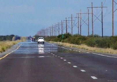
Fresnel is also typicall used as an effect to create soft lighting on the edges (relative to the viewer) of smooth objects. A rough surface, such as a wooden handle that has not been sanded and/or oiled, will not demonstrate the Fresnel effect.

The Fresnel effect is related to refraction of light. We typically think that refraction of light only occurs in liquids, but on the edges of objects some refraction can take place too. Light ray lN coming from light source L would not normally reach the eye of the observer. However, the light ray glances the object and is refracted by the outer layer of the material.
Chapter 6 Lighting 126
6.5 Lighting Calculations
Now that you know the qualitative aspects of the different lighting types it is time to turn our attention to the calculation of diffuse, reflection and Fresnel.
Diffuse lighting
Diffuse lighting is the most straightforward to calculate. You can check the following figure for an indication of the formula that you can use:
PROEFMATERIAAL©VANIN
Notice that as angles α1 to α4 get bigger, the amount of light on the tiles diminishes. In other words, the amount of light on the tile is only determined by the angle between the light vector and the normal As you may suspect, the light intensity can be calculated by using the dot product of the normal and the light vector. The following table shows the calculation for the intensities of the four tiles. Keep in mind that a lower intensity means a darker tile:
The dot formula has been used here to calculate the intensity of the entire tile. The correct term for this type of lighting is flat shading. In games and animation it is possible to calculate the diffuse lighting for every pixel of the screen, which typically results in a gradient colour effect.
2 1 4 3 2 3 4 1
I1 = lN1 n1 = 1 : α1 = 11.35° I 2 = lN2 ⋅ n2 = 0.9 : α 2 = 31.07° I 3 = lN3 ⋅ n3 = 0.7 : α 3 = 45.11° I4 = lN4 ⋅ n 4 = 0.6 : α4 = 54.57°
Chapter 6 Lighting 127
Distance
Sunlight is an important factor in games and with the dot product formula it is possible to calculate the diffuse lighting of sunlight. For sunlight the distance to the sun can be considered constant. The light calculation does not change, whether you are standing on a mountain or at sea level. For spotlights. however, this distance is important and follows what is called an inverse square law. Light source L (e.g. a spotlight) shines in all directions at source strength S (in games or simulations the unit for S can be whatever the game engine or renderer prefers).
PROEFMATERIAAL©VANIN
Point P1 is at distance 1 and will receive light at an intensity equal to:
Point P2 is at distance 2 and its intensity will be equal to:
Finally for point P 3 at distance 3, the intensity will be equal to:
1 2 3
1 = 4 2 = 4
2
= 4 2 = 8
3
4 2
36 Chapter 6 Lighting 128
=
=
Overview and 3D example
The necessary calculations for diffuse lighting can be summarized as follows in the case of a light source that models a sun:
• Determine the light vector (from point P to light source L ) and normalize this vector.
• Determine the normal vector of the triangle.
• Calculate the dot product of the normal vector and the light vector and multiply by the source strength of the sun.
If the light source models a spotlight, you need to take the following steps:
• Determine the light vector (from point P to light source L ) and normalize this vector. Also, determine the distance between point P and light source L and call it distance r.
• Determine the normal vector of the triangle.
• Calculate the dot product of the normal vector and the light vector.
• Calculate the maximum intensity by using the formula: = 4 2
The following figure demonstrates the steps for a spotlight:
PROEFMATERIAAL©VANIN
The distance between lightsource L and P is used to decrease the intensity of the light. We call this distance r and it is calculated using the following formula: r = |L – P |
The maximum intensity at point P is then calculated using the inverse square law:
The light intensity on P is then the multiplication of this maximum intensity and the dot product of the light vector and the normal vector: I D = I M ( lN ⋅ nN)
= 4 2
Chapter 6 Lighting 129
Diffuse lighting examples without distance
In the following example, the distance is not taken into account. For each point on the sphere, the dot product at that point is calculated using light vector lN . It is possible that this dot product is negative, so when calculating lighting (or when implementing them in shaders), it is necessary to check for (and clamp) negative values.
This example does not use the inverse square law to reduce the lighting over distance. The intensity of the light does not fade, so the sphere that is further away from the light receives the same amount of light as the sphere in front.
Diffuse lighting example with distance
PROEFMATERIAAL©VANIN
When using the distance formula (in other words the light is a spotlight), the light intensity diminishes with the square of the distance. For reference, the distance between L and S1 is equal to 1.9 units. You can see that, even with a source strength set to 50, the light output is reduced to practically nothing, even over short distances.
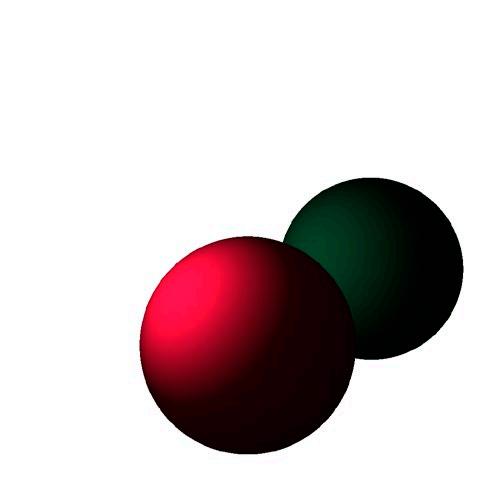
This example uses the inverse square law formula. Notice how the second sphere receives almost no light at all, while the sphere in front receives a lot of light. The source strength is set to 50, while the distance between the light and the first sphere is about two 2 units.
1
1
Chapter 6 Lighting 130
Specular lighting
Specular lighting is the reflection of a light source on an object. Some of the reflected light will be directed towards the viewer, or the virtual camera. An important part of specular lighting is to calculate such a reflected vector.
Another technique for specular reflection is the halfvector technique, which is a lot easier to understand and bring into practice.
Reflecting a vector over a normal
Before you can use specular lighting, you need to understand how to reflect a vector from a surface. The example shows how you can do this in 2D, but the algorithm is set up in such a way that the resulting formula can also be used in a 3D situation.
• P: The point on a surface where a vector will be reflected.
• L: The position of the light.
• lN: The unit vector that indicates the light direction.
• nN: The normal of the surface, which is also a unit vector.
PROEFMATERIAAL©VANIN
We calculate the projection of lN on vector nN using the dot product: h = lN ⋅ nN = cos(α)
ℎ
Chapter 6 Lighting 131
We can now use length h and create a vector: v h = –h * nN v h
is a vector with length h, but it is antiparallel to the normal vector nN. In other words, vector nN is pointing away from the surface, while vector v h is pointing towards the surface.
PROEFMATERIAAL©VANIN
Adding vector v h a second time, creates mirrored vector lM: lM = lN – 2 h nN
This mirrored vector is interesting, but it is not yet what we want. You can flip this vector to generate the desired reflected vector.
The final reflected vector lR can be calculated by flipping vector lM: lR = – lM
ℎ ⃗ ℎ ℎ ⃗ ℎ ⃗ ℎ ℎ
Chapter 6 Lighting 132
To summarize, you start with a light at a position L that shines on a point P of a surface. The normal of this surface is given as n N . The first step is to calculate the normalized light direction: = ( ) | |
PROEFMATERIAAL©VANIN
The next step is to calculate the dot product of this light vector and the normal. Note that this also corresponds to the diffuse intensity:
h = lN ⋅ nN
The mirrored vector is the light vector minus two times the scaled normal:
lM = lN – 2 h nN
And the reflected vector is the flipped version of the mirrored vector:
lR = – lM = – (lN – 2 h nN ) = 2 h nN – lN
Specular lighting in 3D
To calculate the specular light intensity you can use the mathematical method of reflecting a vector. For this technique to work you need to reflect the light vector over the normal. The dot product of this reflected vector and the view vector is then used to calculate the specular light intensity.
In constrast to diffuse lighting, the reflection technique is dependent on the position of viewer E:
To calculate the specular effect with the reflection technique you reflect light vector lN on the triangle via the normal nN .
Chapter 6 Lighting 133
To get the reflected vector you use the formula that was derived in the previous section for 2D situations:
lR = 2 ( lN ⋅ nN ) nN – lN
PROEFMATERIAAL©VANIN
The specular effect is view dependant. It is necessary to take the camera position at E into account, as well as vector e N from points P to E. The specular intensity is now the dot product of l R and vector e N: I s = e N ⋅ lR = 0.73
Example
The specular effect can be seen as the light reflecting towards the camera (or the viewer). Depending on the material there will be a strong specular effect (for example for metals) or a weak one (matte objects, such as wood, plaster, ...).
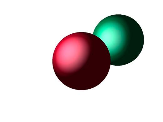
This example uses the reflection formula as shown in the previous section. Obviously something went wrong with this calculation, as both spheres are emitting too much light.
There is too much light shining on both spheres. In the next section you will see a simple operation that can reduce this light output from the specular effect.
Chapter 6 Lighting 134
Shininess
There is one problem with the specular lighting effect as demonstrated in the previous section. By using the dot product of the reflected vector and the view vector, the calculated intensity is too high.
The dot product is propertional to the cosine of the angle between the vectors, as shown in the following figure.
As an example you can derive what the between the vectors would be for a specular intensity of 75%:
PROEFMATERIAAL©VANIN
⋅ = ( )
This picture shows that for a large angle between the view vector and the reflected light vector, the specular effect is too bright if we use the dot product as is. The solution is to raise the cosine function to a power. Remember that the cosine results in a value between –1 and 1. When you raise such a number to a power higher than 1, the result is that the number becomes smaller. This explains the fact why with higher powers you create functions that reach zero more quickly.
⋅ = ∗ ( )
Consider function A * cos(α) S where S is the glossiness. In the figure S is equal to 1, 10, 50 and 100 for the four functions.
A is equal to the specular level, which controls the strength of the specular highlight. This value has been set to 1 in this figure.
cosα
α
arccos
α
41.41° -30∘ -15∘ 0∘ 15∘ 30∘ 45∘ 60∘ 75∘ 90∘ 105∘
= 0.8
=
(0.8)
=
-30∘ -15∘ 0∘ 15∘ 30∘ 45∘ 60∘ 75∘ 90∘ 105∘
Chapter 6 Lighting 135
If you take a look at the intensity of those four functions at the same value for the angle you get:
cos (41.41°) = 0.8
cos (41.41°)10 = 0.1
cos (41.41°)50 ≈ 0
cos (41.41°)100 ≈ 0
So for a specular power or shininess of 10 the light output is already more reasonable. For larger powers this value even drops to close to zero.
Remember that the specular lighting discussed here is part of a simplified model of lighting. The power function can even introduce artefacts when used for rendering games and graphics. The PBR model has better solutions for this problem.
Example
Various specular power values (or shininess values) have been used in the following rendering. The more sizable the area where the specular effect is visible, the smaller the specular power value.
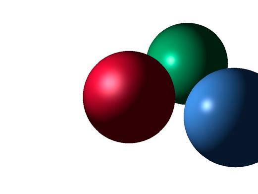
This example uses the reflection formula as shown in the previous section with the shininess value being the parameter for the power function. For the specular effect the dot product is used in combination with unit vectors, so the result of the dot product can only be between –1 and 1
PROEFMATERIAAL©VANIN
By clamping the value between 0 and 1 and increasing it to a power higher than or equal to one, the light output can only get lower.
In this example, the inverse square law for the distance has not been used. When using a spotlight, the light falloff must be taken into account.
Chapter 6 Lighting 136
Halfvector technique
An alternative for the specular lighting is the halfvector technique. Instead of calculating the reflected light vector, a vector halfway between the light vector and the view vector is calculated.
To calculate the specular effect using the halfvector technique we calculate the vector between vector l N and vector e N.
PROEFMATERIAAL©VANIN
To calculate the halfvector we first calculate the sum of e N and l N: h = l N + e N
Note: This vector is NOT a unit length vector, so you need to normalize.
⃗ ℎ
Chapter 6 Lighting 137
The normalized version of h is vector h N
PROEFMATERIAAL©VANIN
The specular effect is view dependant. Vector e N is defined as the normalized vector from points P to E. The specular intensity is then the result of the dot product of vector h N and the normal of triangle nN: I s = h N ⋅ nN = 0.94
The same specular power values (or shininess values) have been used in the following rendering of the halfvector technique. The technique results in highlights that are slightly different from those using the reflection technique, and the highlights are slightly larger and more elliptical.
ℎ ℎ
Example
Chapter 6 Lighting 138
6.6 Fresnel
• When light hits a surface, some of the light gets reflected and some of the light gets refracted.
• The Fresnel equation gives us the percentage of light that gets reflected, based on the view angle. Based on the ratio of reflection and the conservation of energy, we can obtain the amount of refracted light.
We start with the reflection of light on a plane.
PROEFMATERIAAL©VANIN
Some of the light will refract (think about water), and this light will continue in the medium as shown by vector l Refr
The angle will be different from angle α and the ration of the sine of and ϴ is defined as Snell’s law: = ( ) ( )
Chapter 6 Lighting 139
Fresnel edge detection
To calculate the Fresnel effect for smooth objects you need a way to detect edges in the scene. Fortunately, there is again an efficient way by using the dot product
Given is a circle, which is an object that you want to render, and camera point of view E. Consider point P1, which seems to be an edge of the object as seen from viewpoint E.
PROEFMATERIAAL©VANIN
Vector e N is the view vector and vector nN is the normal vector in this point.
Intuitively you can see that the angle between these two vectors is approximately 90°.
The dot product is defined as :
= e N ⋅ nN = |e N| |nN| cos(α) = 0.02
• You see the back of an object if e N ⋅ nN < 0
• If e N ⋅ nN = = 0 then the camera vector is perpendicular to the normal. Around this spot there is a lot of Fresnel effect.
• You see the front of an object if e N ⋅ nN > 0
1 1 1
Chapter 6 Lighting 140
d
The dot product of the view vector gives you an efficient way to calculate whether or not a point of an object is on an edge relative to the camera. You can change the formula to get a 1 as a result when a point is on an edge in the following way: edge = 1 – e N ⋅ nN
The advantage is that the further away a point is from the edge, the lower the result of this formula will be.
PROEFMATERIAAL©VANIN
Fresnel effect
The Fresnel reflectance function is an approximation of the actual physical model. The function presented here is called the Schlick approximation, which is commonly used in PBR (physically based rendering) techniques.
Point E represents the position of the camera.
Vector e N is the unit vector from point T to camera viewpoint E
The Fresnel intensity is the result of the following formula:
I F = F0 + (1 – F0) (1 – e N ⋅ nN)5 with F0 = 0.04
For a non-metallic object, you can use this intensity to create a (grayscale) colour with:
C F = (I F I F I F )
You can add this colour to the final output of the rendering of a particular pixel.
Chapter 6 Lighting 141
Fresnel values and functions
Fresnel values are determined by experiments and this makes it possible to look up values when you need to define materials for games or animations. The value can be different for the red, green and blue channels. The following list are a few examples of values for some materials:
• water = (0 .02 0 .02 0 .02)
• glass = (0 .08 0 .08 0 .08)
• copper = (0 95 0 64 0 54)
• gold = (1 0 87 0 61)
• plastic = 0 . 21 to 0 . 25
The F0 -value is also the Fresnel reflectance at 0°. For metallic surfaces (as shown above) there can be different values for the RGB channels. For non-metallics the value is the same for all channels. To read the functions you need to realise that at 0° the camera vector is parallel with the normal, and at 90°, the camera vector is orthogonal to the normal. So, at 90° there is an intensity of 1
The figure shows different values for F0. A lower value for F0 means that the function starts at a lower value at 0°:
To calculate the output of the Fresnel effect, you first calculate the Fresnel intensity of metals for each colour:
One way to use these intensities is to add them to the the final output colour by combining the red, green and blue values: (I FR I FG I FB). This is not necessarily the most correct way (compared to the PBR workflow), but it already demonstrates the concept of what you can expect from Fresnel reflectance.
-5∘ 0∘ 5∘ 10∘ 15∘ 20∘ 25∘ 30∘ 35∘ 40∘ 45∘ 50∘ 55∘ 60∘ 65∘ 70∘ 75∘ 80∘ 85∘ 90∘ 95∘ 100∘ ( )
I FR = F 0R + (1 – F 0R) (1 – e N ⋅ nN)5 I FG = F 0G + (1 – F 0G) (1 – e N ⋅ nN)5 I FB = F 0B + (1 – F 0B) (1 – e N ⋅ nN)5
Chapter 6 Lighting 142
PROEFMATERIAAL©VANIN
Adding Fresnel reflectance
In the following figure the Fresnel effect has been added to two spheres. The sphere closest to the camera uses Fresnel values of (0 .1 0 .1 0 .1), which tries to approximate water, and the sphere behind it uses a Fresnel value of (0 .9 0 .6 0 .5), which is closer to copper. The Fresnel effect has been exaggerated somewhat to make clear that it adds an edge effect to the rendering of the spheres.
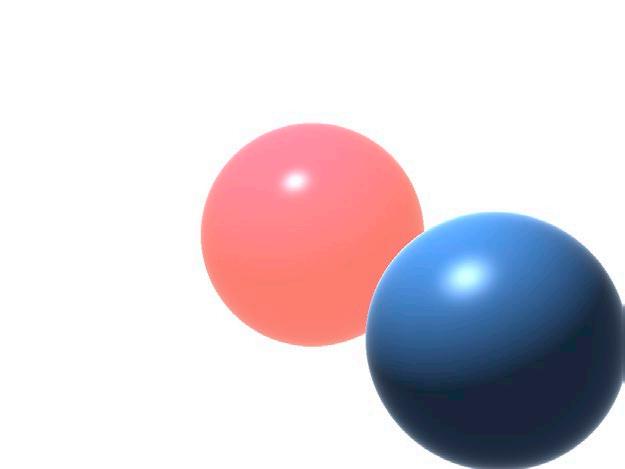
The final effect of the sphere will be determined by:
Diffuse
The diffuse component of the rendering is determined by the colour of the sphere itself and the diffuse intensity:
I D = clamp (lN ⋅ nN, 0, 1)
C D = I D * (C R C G C B)
For the two spheres the colours are red and blue, but it is, of course, also possible to use textures when rendering. Notice again that you clamp the result of the dot product between 0 and 1 to avoid negative values, which would result in different colours.
Specular
For specular you can choose between the reflection technique or the halfvector technique.
Reflection technique
PROEFMATERIAAL©VANIN
Halfvectortechnique
= 2 ⋅ = ⋅ ℎ = + + = ℎ ⋅ Chapter 6 Lighting 143
In both cases, shininess parameter S is used as a power for the dot product. This power function decreases the light output of the specular effect and also creates a smaller highlight area. The I S value can then be used to create a new colour. One way to do this is to use the colour of the light source, as it is the photons of the spotlight, for example, that are reflected from the source.
PROEFMATERIAAL©VANIN
Again, as with the diffuse calculation, the dot products in the final calculation of I S can be negative, so it is necessary to clamp them between 0 and 1 before using the power function.
Fresnel
As mentioned before, you need to calculate the Fresnel intensities for each channel (which is easier if the Fresnel base values F0 are the same):
Then you can use these intensities to create the Fresnel colour:
These values are often used as they are, without multiplying them by other colours.
Final colour
The final colour is obtained by adding the three calculated colours together:
The formulas presented here are not in accordance with the PBR workflow, but offer insight into the process of rendering a simple effect. PBR techniques, formulas and how to combine them are an interesting topic on their own, and if you are interested in shader programming they are definitely worth a look.
C S = I S * (L R LG L B)I FR = F 0R + (1 – F 0R) (1 – l N nN)5 I FG = F 0G + (1 – F 0G) (1 – l N nN)5 I FB = F 0B + (1 – F 0B) (1 – l N ⋅ nN)5
C F = (I FR I FG I FB)
C = C D + C S
F
+ C
Chapter 6 Lighting 144
Chapter 7 Animation
PROEFMATERIAAL©VANIN
Animation deals with the concept of moving objects over time, under the influence of forces
The animation can be based on physics in the case of particles, such as smoke, water or fire particles. It is also possible that the animation is based on active behaviour of an agent (a character whose behaviour is determined by a computer algorithm) in a game or simulation. For example, a guard npc (non playing character) who walks around a fort and potentially chases enemies away.
You start the journey with the basics for all motion: the velocity and acceleration formulas. In most physics courses the entire trajectory is a major topic, but in games and animation, it is important to apply the typical formulas frame by frame. For games you are only interested in the new positions and velocities of objects and characters within a short time window, which is determined by the number of frames per second in the game or animation.
You will again use vectors to model the motion of objects and discover that independence of motion along the X , Y and Z axis of the virtual world is an efficient way to model animations.
Acceleration follows the laws of Newton, so it is necessary that you also understand the basics of composing forces as vectors. Another element is the decomposition of forces into directions that are useful, such as creating vectors that are parallel or perpendicular to the slope of a mountain. This allows you to model the effect of gravity (a force) on an object or character sliding from a slope.
7.1 Velocity
The movement of a particle or object features two properties:
• direction: This is a unit vector that indicates the current direction of the particle or object.
• speed: The speed in units per second. This property tells you how fast an object is moving per unit of time. The units in a virtual world are virtual, but it is a good idea to define a virtual world with meters as the basic unit. The standard time units in a virtual world are seconds
The definition of movement for these two properties makes it possible to control the speed and the direction of a game object independently. This makes it possible to change the direction without changing the speed, or to adjust the speed without changing the direction.
Chapter 7 Animation 145
• The velocity of an object is then created from these two properties as follows: v = S * u with
PROEFMATERIAAL©VANIN
• v : the velocity of the object. This is the multiplication of the speed (in m/s ) by the unit direction.
• S: the speed (in m /s ) of the object.
• u: the unit direction of the object.
Uniform motion
If the velocity of an object is constant and above zero units per second, the object will move in a straight line in a 2D or 3D world. The technical term for this type of movement is uniform motion.
In most highschool programmes, uniform motion is typically described as a one dimensional problem and is typically described as a problem where all the variables are scalars (numbers): d = v * Δt
• with
• d: the distance of the object (in meter).
• v : the velocity of the object (in meter per second).
• Δt : the time (in seconds).
Note: In highschool the symbol s, which is the first letter of the latin word s patium, is used for distance. To avoid confusion with the S variable, denoting speed, you will use the variable d for distance.
The following situation is an example of uniform motion:
• v: 3 m /s
• Δt : 5s
You can calculate the distance d with the formula:
d = v * Δt = 3 m /s * 5s = 15m
This object will travel 15m at a speed of 3 m /s for 5s. Take note of the unit manipulation as well:
m /s * s = m
When starting out with these types of formulas, it is always a good idea to compare the units of your formula with your result to verify that the units make sense.
Chapter 7 Animation 146
Uniform motion with vectors
For games and animations you want to express the problem in a 2D or 3D world, so you need to express the formula with vectors. Fortunately, it is possible to apply the principle of independence of motion which states that movement in a 2D or 3D world can be decomposed along orthogonal axes:
In a 2D or 3D world the movement of an object can be described using orthogonal vectors. In a 2D world you can apply the following formula, which defines the motion along the X and Y axes of the world:
PROEFMATERIAAL©VANIN
You can see (d x d y) and (v x v y) as vectors:
And this leads to the following vector expression:
You need one more adjustment to make this formula useable for games and animations. The vector is the change in position. You will want to use this change in position to calculate the new position of an object after the time period Δt :
= P + d = P + v * Δt with P’ as the new position and P as the previous position
d x = v x * Δt d y = v y * Δt
=
d
v
=
* Δt
Chapter 7 Animation 147
P’
7.2 Velocity
If you want to calculate an object’s movement for an animation, you need to consider the time between two frames of the animation. If you use 24 frames per second (a standard for animation) then the time between two frames (Δt) is calculated as:
1 24 = 0.042
For each frame in the animation you need to consider Δt as it will be used in the position formula:
PROEFMATERIAAL©VANIN
The following figure simulates what would happen in a virtual world if an object has a starting position of P = (1m 1m), a velocity vector vN = (0 .96 0 .3) and a speed of 8m /s . The velocity vector vN is normalized.
In the figure, object P has an initial velocity vector vN, speed 8m /s, no acceleration vector, and starts at position (1m 1m).
The new position can be calculated with the following formula:
1 1 + 0.042 ∗ 8 / 0.96 0.3
In this example, the velocity direction and speed did not change and the object continues to move in the same direction. This can happen in space when a spaceshipe cuts its engines and continues to drift in the same direction. The velocity of an object can only change if you apply a force to this object.
=
0 1
′
′
∗
Chapter 7 Animation 148
= + ∗
=
= 1.318 1.099
7.3 Acceleration
Without acceleration, an object will remain at rest or move at a constant speed. Hence, acceleration can be understood as the change in speed per time unit. A typical example of this is the acceleration test of a car, where the time in which the car goes from 0 km /h to 100km/h is measured. For example, some electric cars can accelerate from 0km/h to 100km/h in 2.3 s, as shown in the following figure:
100 km = 100000m
1h = 3600 s
The plot of the speed over time shows the car’s speed (in kilometers per hour) on the vertical axis and the current time (in seconds) on the horizontal axis. The car starts at 0km /h and has a velocity of 100km /h at time 2.3 s
PROEFMATERIAAL©VANIN
The acceleration is the change in speed Δv in 1 second. You can estimate from the figure that this Δv will be approximately 40km /h per second. In this example, the units are seconds, hours and kilometers, which can lead to confusion and errors. The solution is to convert the data to standard (SI) units, which leads to an accelaration that is also useable in games and animation.
0 1 2 34 5 -10 10 20 30 40 50 60 70 80 90 100 110 120 1 t( ) v( /ℎ ) 1 2 = 100 /
ℎ
Chapter 7 Animation 149
Standard units
To calculate the change in speed with standard units it is necessary to convert all the units to seconds and meters. The speed conversion to <no unit> is:
PROEFMATERIAAL©VANIN
To calculate the acceleration you need to know the start speed (S s) and the end speed (S e):
The difference of these two velocities, divided by the time period of 2.3 s results in the change in speed per time unit, or acceleration:
The unit of acceleration is m/s2 , which is the result of the division of the speed unit being m/s, by the time unit s. In this example, the speed of the car will increase with 12 m /s per second
1 = 100 1ℎ = 100000 3600 ≈ 28 /
S e = 0m /s S s = 28m /s 0 1 2 34 5 10 20 30 40 1 t( ) v( / ) 1 2 1 = 28 /
=
≈
Chapter 7 Animation 150
2.3 = 28 / 2.3
12 / 2
7.4 Animation and Acceleration
Similar to the situation with velocity, you need to use vectors in games for calculating the position update for each frame of the animation. It is important to know the difference between different visual presentations of the same concept.
Uniformly accelerated motion
There are different ways to setup formulas for speed and acceleration. The formula that most people start out with describes how the position changes in one dimension over time.
The figure shows a position-time graph. The horizontal axis is the time axis in seconds. The vertical axis presents the current position of the object.
This graph shows the height of an object over time under the influence of gravity:
PROEFMATERIAAL©VANIN
In this example the value of y0 is 10m. From the plot you can read that the height of the object is approximately 5m after 1s
A typical question to ask is when the object will reach ground level. In other words, what is the value of t when y = 0 m? To solve this you first determine which elements of the formula are known. From the plot you can read that the y value equals 10 begingroup m at t = 0 s. The variable g corresponds to the gravitational acceleration on earth:
-0.4-0.200.20.40.60.8 11.2 1.41.6 -1 1 2 3 4 5 6 7 8 9 10 11 12 ( ( ) 1 ≈ 5.095
y = 0m y0 = 10m g = 9.81 m /s2
= 0 2 2
Chapter 7 Animation 151
If you use these values in the equation you get:
PROEFMATERIAAL©VANIN
The value for t can be found on the plot where the position-time graph intersects with the horizontal axis. You can visually verify this on the plot above.
XY-graph
The position-time graph is useful if you are mainly interested in one-dimensional problems and want to predict special events (e.g. falling on the floor, hitting a wall...) related to the motion. Another way to visualize the motion is to create an XY-plot of it. This plot can show the movement of an object in 2D and even 3D space, but you lose the visualization of time
The picture shows an XY-plot with the start position given as:
P S = (2 m 3m). The start speed in the x-direction is equal to 3 m /s and the speed in the y-direction is equal to 0m /s. The velocity vector v is then equal to (3 m /s 0m /s).
The gravitational acceleration is equal to –9.81 m /s2
To setup the equation you use the uniform motion formula for the x-direction and the uniformly accelerated motion formula for the y-direction. In other words you apply the principle of independence of motion to split up the problem in a horizontal and a vertical part.
= 0 2 2 ⇒ 0 = 10 9.8 2 2 ⇒ 9.8 2 2 = 10 ⇒ 2 = 20 9.8 ⇒ = 20 9.8 = 1.428
X( ) Y( ) ⃗
= 0 + ∗ = 0 ∗ 2 2
Chapter 7 Animation 152
For the XY-plot you try to get rid of the variable t and the easiest way to do this, is to isolate t in the first equation:
PROEFMATERIAAL©VANIN
You can then plug this formula for t into the second equation:
This formula gives you a quadratic equation in x, which results in the parabolic shape you see in the figure.
Change in velocity without time
It can be useful (as you will see when implementing the jump of a game character) to use a formula that can calculate the change in velocity based on a distance and a value for the acceleration only. You can start with the following two formulas:
In the first formula you isolate t :
You can then apply that t-variable in the second equation:
= ( 0 ) = 0 ∗ 2 2
⎧ ⎪ ⎨ ⎪ ⎩ = ( 0 ) = 0 2 ( 0 )2 2
1 = 0 + ∗ = 0 ∗ + ∗ 2 2
= 1 0
= 0 ∗ ( 1 0 ) + ∗ ( 1 0 )2 2 ∗ 2 Chapter 7 Animation 153
Putting all the numerators to 2 * a and working out the squares leads to:
PROEFMATERIAAL©VANIN
The formula is typically expressed in the following form:
With this formula you can answer one of the following questions:
• Given the distance (or height) what is the starting velocity of the object under consideration?
• Given the start velocity, what is the height that the character will reach?
Working in one dimension
Note that even when you work in one dimension, the position, velocity and acceleration can be expressed using negative numbers. The following example shows two cars racing towards each other, possibly resulting in a crash if neither car chickens out and pushes the brakes, which is a negative acceleration.
The cars’ velocities are:
• Car 1: (0 .6m /s 0m /s)
• Car 2: (– 0 . 5m /s 0m /s)
= 2 ∗ 0 ∗ ( 1 0 ) 2 ∗ + ( 1 0 )2 2 ∗ = 2 ∗ 0 ∗ 1 2 ∗ 0 2 + 1 2 2 ∗ 0 ∗ 1 + 0 2 2 ∗ = 1 2 0 2 2 ∗
v 1 2 – v 0 2 = 2 a d
⃗ 1 ⃗ 2
Car1 Car2
Chapter 7 Animation 154
Even when you decide to work in one dimension (which you are allowed to do thanks to independence of motion), you will still work with the positive and negative values of the x-components of the vector values:
• Car 1: 0 .6m /s
• Car 2: – 0 5m /s
Keep this in mind when working with gravity, as these types of problems are also typically formulated in one dimension, but with the gravity acceleration begin negative. The next section demonstrates this concept of a negative gravitational acceleration.
Distance exercise
Typically the formula is applied in the following case:
PROEFMATERIAAL©VANIN
The problem is to calculate the initial vertical speed for the character to make sure that the character jumps 3m high (assuming earth gravity). The following formula was made for these types of situations:
v1 2 – v0 2 = 2 gd
It is important to keep in mind that the speed of the character will be zero at its highest point:
v1 = 0m /s
With g being a negative value (downwards) the start velocity can be calculated as:
0 = 2 = 7.672 /
The speed in kilometers per hour for this jump is about 28km /h, which is impossible for mere mortals, but, depending on the game genre, entirely possible.
=
3
Chapter 7 Animation 155
Frame by frame animation
In physics the position-time graph is conventionally used to present motion. However, this is not the way motion is implemented in games and animations. A first major difference is that the motion will be represented in a 2D or 3D world by points and vectors. A second difference is that in a game or animation the motion will be calculated frame by frame. It is very rarely the case that the full path of an object is necessary for a longer time period. Instead of a formula where speed and acceleration is combined, you will typically use a separate position and speed update for each frame. Remember that the start velocity can be calculated by multiplying a speed by a unit direction:
v0 = S u
The relevant formulas to update the position and velocity are:
v1 = v0 + g Δ t
P 1 = P 0 + v1 Δ t
An important detail here is that the new velocity will be immediately used for the position update. These two formulas will be used each frame to create the object’s motion. A practical example in 2D will give you more insight in this process. You start with the values at t = 0 s for the object. The object is given a speed of 5m /s and a direction of (1 0). This direction represents an initial horizontal motion of the object. The initial position of the object is at (0 5 1).
S = 5m /s
u = (1 m /s 0m /s) v0 = S u = (2 m /s 0m /s)
Finally the frames per second (fps) of the game or animation will determine the value of Δt. You can use the default frame rate for animation of 24fps: = 1 24 = 0.042
Simulation
The calculation of the position and velocity updates for a couple of frames is tedious work, but it is important to get a good grasp of the process:
Frame 0
v0 and P0 are given, so the position and velocity of the object are: v0 = (2 m /s 0m /s) P0 = (0 . 5m 1m)
g
81 m
P
= (0m /s2 –9
/s2)
0 = (0 . 5m 1m)
Chapter 7 Animation 156 PROEFMATERIAAL©VANIN
Frame 1
The elapsed time from frame 0 is 0.042 s and you now apply the two formulas to update the position and velocity:
PROEFMATERIAAL©VANIN
This v1 value is used right away in the position update:
Frame 2
The same process is repeated for frame 2, but you now use the position and velocity that were calculated in frame 1:
Notice how the horizontal velocity v x does not change during this simulation. This is because the acceleration vector g only has a component in the vertical direction.
Simulation results
The figure below shows the results of this simulation. Notice how the velocity vectors and the points have changed compared to the previous frame. By updating the velocity vector each frame, the gravitational acceleration pulls down the velocity vector. A couple of extra points have been added to this figure to demonstrate that this simulation creates a curve that is similar to a horizontal throw
The time variable is not visible in this plot, as this is a XY-plot of the motion. The time that has passed between each point however, corresponds to 1 24 = 0.042
⃗ 1 = ⃗ 0 + = 2 0 + 0 −9.8 0.042 = 2 / −0.409 /
1 = 0 + ⃗ 1 = 0.5 1 + 2 / −0.409 / 0.042 = 0.583 0.983
⃗ 2 = ⃗ 1 + = 2 −0.4 + 0 −9.8 0.042 = 2 / −0.818 / 2 = 1 + ⃗ 2 = 0.583 0.983 + 2 / −0.818 / 0.042 = 0.667 0.949
X( ) Y( ) ⃗ 0 ⃗ 1 ⃗ 2 0
.
Chapter 7 Animation 157
7.5 Laws of Newton
The laws of Newton offer a framework for solving problems that have a physical basis. The main goal in games and animation is to apply forces and momentum to objects with parameters that can easily be tweaked. Working with a physically based approach is important to reduce the amount of time spent fiddling with various parameters.
First law
The first law states that objects have a constant velocity. The velocity can only change if a force is acting on the object.
A body that is in motion wants to stay in motion. A body at rest wants to stay at rest.
For this law you can imagine a spaceship that has lost its propulsion systems drifting in space, far away from other planets, stars or other objects in the universe that can exert a force. Without forces acting on the spaceship it will move with the same velocity (direction and speed) until it encounters a force that changes its direction.
Second law
This law states that if a change in velocity occurs, a net force must have been exerted on the object.
An acceleration (change in velocity) can only occur if a force is applied to an object.
The term net force is important here. There might be multiple forces acting on an object, but if the sum of the forces is the zero vector, there will be no change in velocity.
Forces are represented as vectors and all the operations that apply to vectors, such as adding, multiplication by a vector, dot product, ... also apply to forces. The concept of independence of motion applies to vectors as well. If you can decompose a force into two orthogonal vectors in 2D space, then you can consider the effect of each orthogonal vector separately. You will apply this concept in the section about the object on a slope under influence of gravity. Given: F1 = (2 0)
= (–2 0) F1 + F2 = (0 0)
⃗ 1 ⃗ 2
Chapter 7 Animation 158
F2
PROEFMATERIAAL©VANIN
Force is defined as the multiplication of the mass (in kilograms) of the object by the acceleration:
F = m a
The unit of force is the Newton (abbreviated N ).
PROEFMATERIAAL©VANIN
Third law
Newton’s third law connects the dots between the first two, making it a key component for addressing various physical challenges, such as collisions between objects, handling movement on a slope under influence of gravity, ...
Every action is followed by an equal but opposite reaction
Imagine an object that is motionless on the ground on some planet. Motionless implies that the velocity is equal to (0m /s 0m /s).
Say the force acting on the object is the gravitational force of the planet that is pulling on the object. However, it is given that the object does not move, which is a contradiction. If the object does not move, the sum of forces must be (0N 0N ).
There must indeed be a force FR that cancels out the gravitational force F g : FR + F g = (0 N 0N )
With the sum of forces being the zero vector, there will be no acceleration (second law) and the object will remain at rest (first law).
Intuitively, if the ground would not push back with the same but opposite force as the gravitational force, the object would be accelerated into the ground, which can indeed happen if the ground were to turn into a liquid.
⃗ ⃗ ⃗
Chapter 7 Animation 159
Force example
Forces are used in many game engines to control the movement of objects. If a game or animation uses a physics engine under the hood, applying a force to an object is a physics friendly way to control the acceleration and velocity of this object. There is only acceleration as long as the force is present. For example, when hitting a golfball with a golfclub, you apply a force to the golfball. However, when the golfball breaks contact with the golfclub the acceleration of the golfball ceases. From that point on, the ball continues to move due to its inertia, travelling in the direction it was sent until other forces, such as gravity, wind, air resistance, and friction, act upon it to alter its trajectory or bring it to a stop.
For a first example, imagine a ball rolling over a flat surface. The ball has a mass of 0.1kg and a speed of (3 m /s 0m /s), in other words the ball is moving in the horizontal direction. A fan is blowing in a vertical direction, so when the ball enters the area where the fan is blowing, there will be an acceleration effect on the ball.
PROEFMATERIAAL©VANIN
The force in Newton is 0.4N and expressed as a vector: (0 N 0 .4N ). The second law of Newton states:
As long as the ball stays in the area where the fan is blowing it will accelerate.
2 1 fan ⃗ ⃗ ⃗ ⃗
⃗ = = ⃗ = 0 0.4 0.1 = 0 / 2 4 / 2
Chapter 7 Animation 160
Time period
The first problem you need to identify is when the ball will enter the wind zone and how long the ball will stay in this zone. Because of independence of motion you only need to take the horizontal velocity of the ball into account: v = (3 m /s 0m /s)
The time will be the horizontal distance divided by the horizontal velocity:
PROEFMATERIAAL©VANIN
The ball enters the windzone after 1m so the time it takes for the ball to enter the wind zone is:
When the ball enters the windzone it stays in this zone for 2m , so the time that the ball stays in the windzone is:
From this calculation you can conclude that the wind force will be applied to the ball for 0.667s. As the wind is applying a force in the vertical direction, only the vertical velocity of the ball will be affected.
Force and acceleration
For animations and games you need to apply the formulas frame by frame. The animation starts at t = 0.333 s, when the ball is at position (2 m 1m) and has just entered the wind zone.
The framerate of the animation is again set at 24fps and the time between two frames is then: = 1 24 = 0.042
You again apply the two following formulas to calculate what will happen in the next frame:
= ⇒ =
1
1
1 3
0.333
=
=
/ =
2 = 2 = 2 3
= 0.667
/
⃗ 1 = ⃗ 0 + = 1.5 0 + 0 4 ∗ 0.042 = 1.5 / 0.167 / 1 = 0 + ⃗ 1 = 2 1 + 1.5 / 0.167 / ∗ 0.042 / = 2.062 1.007 Chapter 7 Animation 161
Simulation
If you repeat this process for a sufficient number of frames you can trace the path of the object. The horizontal distance between two positions is constant, as the horizontal velocity is not affected by the wind force. The vertical distance increases because the vertical velocity is impacted by the wind force:
PROEFMATERIAAL©VANIN
When the ball leaves the wind zone there is no force acting on it, so the ball will keep rolling in the direction of the velocity vector v . On earth the ball will eventually stop due to friction. The visualization here is again an XY-graph without time. It is however possible to determine the time, as the time difference between two locations is equal to Δt.
fan ⃗ ⃗ ⃗ ⃗
Chapter 7 Animation 162
Gravity on a slope
Consider a skier on a slope, represented by point P. Gravity force F g is pointing downwards.
Question: How can we calculate the effect of gravity on an object on a slope?
The first step is to consider the angle β of the slope. This angle will of course have an effect on the acceleration and speed of the skier.
PROEFMATERIAAL©VANIN
The second step is to project the gravity force vector F g on the slope. The important question is now what the x and y components of this projection will be.
⃗ ⃗ ⃗
Chapter 7 Animation 163
When we project vector F g on the slope, we know the angle between F g and F p because:
α + β = 90°
α = 90° –β
To calculate the length of vector F p we can now again use the right angle formulas (CAH):
PROEFMATERIAAL©VANIN
We now have the length of the vector F p and its angle β , so we can conclude:
= ⃗ ( ) ⃗ ( )
With force vector F p known, it is now possible to calculate acceleration vector a because:
where m is the mass of the skier or the object.
⃗ ⃗ ⃗ ⃗
(
) = ⃗ ⃗ ⇒ ⃗ = ⃗ ( )
⃗
= ⃗
Chapter 7 Animation 164
Finally, there remains a perpendicular part of the force, which we name F⊥. This force has to be there because otherwise a part of gravity vector F g would have disappeared. Force F⊥ pulls the skier or object towards the slope.
PROEFMATERIAAL©VANIN
Force F⊥ pulls the skier against the slope, but a reaction force (Newtons third law) of the slope itself ensures that the skier does not sink into the ground.
⃗ ⃗ ⃗ ⊥ ⃗ ⃗ ⃗ ⊥ ⃗
Chapter 7 Animation 165
7.6 Energy
Conservation Law
Energy is a fundamental concept that permeates every aspect of the physical universe, underpinning the very fabric of existence. It manifests in various forms, such as kinetic energy associated with the movement of objects, potential energy stored within objects due to their position or arrangement, thermal energy related to the temperature of an object, and many other kinds, including chemical, nuclear, and electromagnetic energy.
The principle of conservation of energy, a cornerstone of physics, states that energy can neither be created nor destroyed, only transformed from one form into another.
Physics engines in games apply this principle when simulating physical reality. When collisions between objects occur in a game, the total amount of energy should remain constant.
Physically based rendering is another field in game development and rendering where this principle is very important. When light illuminates an object, the reflected light cannot be more intense than the source of the light. Ultimately, all energy is derived from the motion of fundamental particles.
Energy formulas
Energy is expressed in Joules ( J ). The kinetic and potential energy formulas help with converting the energy to velocity and vice versa.
One Joule is defined as the amount of energy expended when a force of one Newton is applied over a displacement of one meter. In mathematical terms, 1 Joule is equivalent to 1 Newton-meter ( Nm ) in the context of mechanical work or energy.
Kinetic energy is the energy that is associated with the motion (velocity) of an object:
PROEFMATERIAAL©VANIN
m is equal to the mass of the object in kg and v the speed of the object in m /s .
Potential energy is the energy that is stored in an object in the gravitational field of a planet. The formula for potential energy is:
Again m equals the mass of the object in kg, h the height of the object in m and g the absolute value of the gravitational acceleration constant in m /s2
= 2 2
E p = m * |g| * h
Chapter 7 Animation 166
Potential and kinetic energy example
The following example demonstrates the potential and kinetic energy formulas, while also highlighting the principle of conservation of energ y.
Let there be an object with mass 2 kg suspended over the ground at a height of 2 m. The object is a sphere with radius = 0.25m. The sphere has a centerpoint, which in physics is typically called the center of mass
The goal of the example is to calculate the velocity of the object when it hits the ground. In order to do so, you need to take the radius of the object into account when calculating the height of this object. Subtracting the radius from the height from the center of mass of the ball to the ground results in h = 1.75m.
The object has a potential energy wich is represented by:
PROEFMATERIAAL©VANIN
When the ball hits the ground all of its potential energy has been converted into kinetic energy.
With both formulas, you can now calculate the velocity of the ball when it hits the ground. The potential energy formula calculates the energy that the ball has when it is suspended in the air, the kinetic formula results in the energy that the ball has when it hits the ground:
This problem can also be solved with the kinetic formulas, but the interesting aspect of this solution is that it is not necessary to calculate the time it takes for the object to fall from its position at h = 1.75m to ground level.
ℎ = 1.75
= ⇒ ∗ 2 2 = ∗ ∗ ℎ ⇒ = ∗ ∗ ℎ (2 ∗ ) ⇒ = ∗ ℎ 2 = 2.072 /
E p = m * g * h = 2 kg * 9.81 m /s2 * 1.75m = 34.335J
Chapter 7 Animation 167
7.7 Momentum
Another consequence of the energy conservation law is the conservation of momentum.
PROEFMATERIAAL©VANIN
Definition of momentum
Momentum is the product of the mass of an object times the velocity of an object. The letter that is used for momentum is the small letter ‘p’.
p1 = m1 * v1
The unit of momentum is kg m /s . Momentum is a vector quantity, meaning it has both magnitude and direction, which indicates the velocity of the object. Momentum is used for the calculation of collisions in games and animations.
Conservation of momentum
When an object hits another object, momentum is conserved: If v1 and m1 is the speed and mass of an object before the collision, and v2 and m2 is the speed and mass of an object after the collision then the following conservation law can be written: m1 * v1 = m2 * v2 mass * speed = mass * speed
Chapter 7 Animation 168
Collision example
A typical example of the use of the momentum formula is a modified version of Newton’s cradle, which you see demonstrated here. The ball on the left is elevated to a higher position, and when released this ball will follow a circular trajectory and hit the ball on the right.
PROEFMATERIAAL©VANIN
The masses of both balls are equal, so if we assume that the collision is elastic the left ball will be motionless after the collision and the right ball will have a velocity equal to the velocity of the left ball right before the collision.
Chapter 7 Animation 169
7.8 Change of Momentum
When you want to calculate the velocity change of a single game object it can be practical to express the problem as the change of momentum. Important here is that the mass of the object does not change.
For this specific situation you consider the velocity of one object at two different times (t0 and t1). The mass m of the object does not change in this time period:
PROEFMATERIAAL©VANIN
You can now examine the change in momentum in the timeperiod from t0 to t1:
The change in velocity Δv is equal to the acceleration a multiplied with the time period Δt :
1 0
Applying Newton’s second law then gives another expression for the change in momentum: Δ p = F Δt
Combining both forms gives you an easy way to determine the change in velocity when applying a force for an amount of time (given by Δt):
Combining both expressions for the change in momentum leads to the following formula: m Δ v = F Δ t
0 ∶ 0 ⇒ 0 = 0 1 ∶ 1 ⇒ 1 = 1
= 1 0 = 1 0 =
=
( 1 0 )
=
= =
= =
Chapter 7 Animation 170
Change of momentum as vectors
We can now also define the change in momentum as vectors:
PROEFMATERIAAL©VANIN
You can again combine the formulas in the same way you did for the scalar expression. So we get:
Δv = F Δ t
The importance of this formula is that it allows you to calculate a change in velocity when a force is applied to one object over a given amount of time Δt :
Change in momentum equals the average net external force multiplied by the time this force acts. Change in momentum is also called impulse.
Example
A bullet is accelerated down the barrel of a gun by hot gases produced by the combustion of gun powder. What is the average force exerted on a 0.03 kg bullet to accelerate to a speed of 600m /s in a time of 0.002 s?
To solve this problem you start with the formula and write down the elements of the formula that you know, then you isolate the variable that you want to calculate:
Given
• m: the mass of the object is stated as being equal to 0.03kg
• Δv: the change in velocity is not directly stated, but the problem definition implies that the speed of the bullet at … is equal to 0m /s and the speed of the bullet is 600m /s . You can conclude that the change in velocity is 600m /s
• Δt : This is explicitly stated in the problem definition and is equal to 0.002 s
⃗ = ⃗ ⃗ = ⃗
m
⃗ = ⃗
m Δ v = F Δ t
Chapter 7 Animation 171
Question
The problem definition requires force F that was applied to the bullet. The formula has four different variables of which three are known, so it is possible to calculate this value now.
PROEFMATERIAAL©VANIN
Solution
A good first step is to isolate variable F in the formula:
As a last step you replace the variables with their known values:
0.03 600 / 0.002 = 9000
This example is of course a simplification of the actual process. There are several other forces at play in this scenario. For simulations however, this approach would give a good first indication of the actual speed of the bullet as it leaves the muzzle.
The speed of 600m /s given in the problem definition is equal to 2160km /h, which certainly is an impressive speed. The combustion force that accelerated the bullet to this speed, however, is no longer acting once the bullet leaves the muzzle.
This also means that the initial speed at which the bullet leaves the muzzle will drop quickly, mainly due to air resistance. In this scenerio, the two main forces acting on the bullet are gravity (which will cause the bullet to lose height), and air resistance (which will decrease the speed of the bullet).
= ⇒ =
=
Chapter 7 Animation 172
Jumping in games – a comparison
In the context of video games and animations, one of the most common actions a character can perform is a vertical jump. This seemingly simple action is a fundamental element that can define the gameplay experience, influence the game’s mechanics, and significantly impact the overall design. But how do we bring this dynamic motion to life in a virtual environment?
PROEFMATERIAAL©VANIN
Creating a convincing jump requires an understanding of basic physics principles and their application within a game’s engine. Essentially, you are simulating the effects of real-world forces within a controlled digital space. This involves translating the force exerted by legs pushing off the ground, the momentum carrying the character upwards, and the inevitable influence of gravity bringing them back down to the surface.
An important question to answer when implementing jumps is how realistic do you want the jump to be? Most characters in games have superhuman abilities to make the gameplay more interesting. For example, in the figure above you perhaps want the character to jump on the platform that is 2 m above ground. Given that the record for high jump at the time of writing stands at 2.45m, the game design already veers into magical territory.
A second question: do you want to implement different jumping capabilities or even change the height the character can jump depending on how much this character is carrying? In other words, do you want to consider the mass of the character or other abilities and skills as a factor?
⃗
Chapter 7 Animation 173
Analysis
There are two possibilities to implement the jump. Both methods allow the designer to play with timings and the mass of the character. In most engines it is possible to add an impulse to an object or to add a force to an object. The specific game mechanics and environment of the game determine which method is preferred.
• Impulse method: We implement this as if the character is building up force for a certain amount of … resulting in a velocity at the time of the jump. In other words, the jump is framed within the concept of impulse and momentum. This method is particularly useful when a character only has biomechanical means of jumping at its disposal.
• Force method: We apply a force for a certain amount of time starting at the jump itself. This means that the character will start with a zero velocity and will accelerate upwards for some time. The drawback of this method is that this force will need to be balanced to counter the effect of gravity. The time that the force will be active also plays an important role and needs careful consideration. This method is sometimes used when characters have something like a jetpack to give a small boost to a biomechanical jump.
The method that uses forces is also useful for game elements, such as rockets, that have their own internal propulsion systems.
How to calculate the simulation
The goal is again to implement frame based animation. The Δt is calculated with the game or animation’s frames per second: = 1 24 = 0.042
The calculation is expressed in vectors, but by applying the indepence of motion principle it is possible to break down the calculations into their components. The acceleration a can be the result of multiple forces acting on the object or character with one of those typical forces being the force of gravity.
v1 = v0 + a Δt P1 = P0 + v1 Δt Chapter 7 Animation 174
PROEFMATERIAAL©VANIN
Vertical jump with impulse
A character with a mass of 75kg stands on the ground. The gravity acceleration of the earth g = 9.81 m /s2 is used. The character needs to be able to jump at least 2 begingroup m high. To get a better feeling for the parameters you need to set, you can first calculate the starting speed to be able to reach that high. Here you can use the uniformly accelerated motion formula without t-parameter to calculate this velocity: v1 2 – v0 2 = 2 gd
As with the previous example, the speed v1 when the character reaches the apex of the jump is 0m /s. To calculate the distance you take the difference of y0 which is ground level, and y 1 which is the height of the platform:
PROEFMATERIAAL©VANIN
The velocity of the character when the top is reached is 0m /s, and the formula to calculate the start velocity is: 0 = 2 = 6.264 /
This velocity already gives a good indication of the starting velocity that you need for the character to reach the platform.
To calculate the change in momentum you can use the formula: Δ p = m Δ v = F Δ t
The mass of the character and the change in vertical velocity are known, so it is possible now to calculate the change in momentum:
The change in momentum Δp is also equal to force times time (F Δt ). If you choose the force as1000 N, then the time for this impulse is given by: = = 470 / 1000 = 0.47
0
=
=
⃗
= 0 1 = 2
1 0
2
≈
Δ p = m Δv = 75kg * 6.264m /s
470 kg m /s
Chapter 7 Animation 175
It is important to consider here that the change in momentum gives the game or animation designer a baseline for the jump animation. The force, time and mass parameters for the character can now be finetuned as elements of the game mechanics. Some platforms could be out of reach for game characters that are heavier, or the time for the impulse formula could be controlled by certain abilities or magical effects.
The effect of the starting velocity is shown in the following figure. Lower starting velocities result in a path that reaches a lower apex, and as a result, the horizontal distance travelled will also be smaller:
The three trajectories show the effect of three starting velocities:
= 6.25 / = 7 / = 7.6 /
The path in the middle seems to fit the requirements best.
PROEFMATERIAAL©VANIN
Notice that each path is shown for a duration of about 1s and that each path covers the same horizontal distance. This is again an application of independence of motion since v x has the same value for the three paths.
Vertical jump with force
With this method you simulate what happens if you apply a force of 1000N for 0.5s on the character object with a mass of 75kg. During this period of 0.5s both this force and the force of gravity will be applied to the character. If this force results in an acceleration that is lower than the constant gravitational acceleration on earth, the character will not be able to lift itself from the ground!
First you need to calculate the acceleration during the first 0.5s of the jump: = = 1000 75 = 13.333 / 2
This acceleration is a positive value (accelerating the character upwards), but will immediatly be counteracted by gravity!
1 2 3
Chapter 7 Animation 176
For the first 0.5s the path curves upwards, which could give a weird impression to the player. After this first time period, the upwards force falls away and gravity takes over. Notice that with about the same force and time period, the character will not even get near the platform.
PROEFMATERIAAL©VANIN
Adjusting the parameters
The force of 1000N did not give good results. After experimentation this value has now been set to 1350 N. This results in a path that has a better chance of ending up at the desired location, as you can see in the following image:
Again the first 0.5s might look weird to the player. It is also quite a bit harder to come up with good values for F and Δt.
0.5
0.5
0.5 0.5
Chapter 7 Animation 177
Conclusion
Physics engines are part of the game and animation development process. It is not necessary to implement all the details yourself, as there are quite capable physics engines, such as nVidia Physics, Bullet physics, Havok, and others. It helps however to be aware of the terminology of physics and to be able to do a quick back-of-the-envelope calculation to set plausible parameters for a simulation.
For a regular (non mechanically assisted) jump, the change in momentum method seems better. It is straightforward to implement and the path that the character follows looks realistic.
Adding a force during the jump on the other runs the risk of coming across as not realistic, unless there is a mechanical or magical way that the character can fly or get an upwards boost. As you learned in the discussion about the jump with force, with this method it can be harder to get the result that you need for your game of animation.
PROEFMATERIAAL©VANIN
Chapter 7 Animation 178
Chapter 8
Transformations with Matrices
PROEFMATERIAAL©VANIN
Matrices are used extensively in game engines and modelling software to apply transformations on 2D and 3D objects. The common transformations in games are translation, rotation and uniform scale. A special transformation is the perspective matrix, which adds perspective to a 3D rendering.
The chapter starts with a presentation on the basics of matrix manipulation. First we define what a matrix is and what it represents. The discussion will focus on the operation that is most useful for game development, which is the matrix multiplication, also sometimes called the matrix dot product.
As a next step, you apply the knowlegde about matrices and vectors to create transformation matrices.
The matrix should not be a black box of numbers, therefore it is also important that you can analyse the transformation that is stored inside the matrix.
8.1 The matrix
A matrix is defined as a 2D grid of numbers. An example of a 2 by 2 matrix is given below:
2 by 2 means that the above matrix has 2 rows and 2 columns. An example of a 3 by 2 matrix, meaning a matrix with 3 rows and 2 columns, is the following one:
The first dimension of a matrix is always the number of rows. So, the second dimension of a matrix is obviously the number of columns. To write the size of a matrix we will typically write the number of rows first and then the number columns, with an ‘x’ in between. The first matrix is then a 2 × 2 matrix and the second one is a 3 × 2 matrix. You need to get into the habit of using the number of rows first and then the number of columns. Individual cells or elements within a matrix use a subscript for the row and column within that matrix and instead of the uppercase letter, which is used for the matrix, you use a lowercase letter:
Chapter 8 Transformations with Matrices 179
= 55 117
= 54 117 894
PROEFMATERIAAL©VANIN
As an example, the element on the second row, first column is then the value 11. b21 = 11
The interpretation of what the matrix means, depends on the application. In this chapter we will focus on matrices that can be used to transform vertices. Game engines, 3D editors, and games commonly use matrices to represent transformations, because a single matrix can define precisely where a 2D or 3D object should be rendered on the screen. Matrices make it a lot easier to define the complex translate, scale and rotate operations that are needed to create a game.
The matrix in game engines
A matrix can represent many mathematical constructs. For graphical applications, however, a matrix typically represents a transformation (translation, rotation, scale, camera or perspective transform). To explain this concept we demonstrate the usage of matrices in some typical game engines. In the Unity game engine, a transform is typically defined by a position, rotation and scale:
This transformation is internally defined as a matrix. In the screenshot from Unity the transformation is defined as follows (with the rotation given in degrees):
position = ( 1 2 3)
rotation = (0° 26° 0° )
scale = (1 1 1 )
To convert these transformation data to a matrix, some calculations (which will be explained in later sections) are necessary. For the cabana in the screenshot, the matrix would be:
= 11 12 21 22 31 32 = 54 11 7 894
Chapter 8 Transformations with Matrices 180
Chapter 8 Transformations with Matrices
PROEFMATERIAAL©VANIN
From this equation it is easy to deduce that you need trigonometric functions to calculate the rotation (which will be explained in the section about rotation). The scale (1 1 1) is encoded in the matrix, but not directly readable, and as mentioned, the position can be directly deduced by reading the last column of the matrix.
The matrix in Blender
Matrices are also used internally in 3D editors. For example, in Blender it is possible to manipulate the transformation of an object by directly manipulating its transformation matrix.
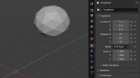
The internal matrix transform for the object shown, can be queried via the Python language in Blender applying the following command:
, 0.4383711516857147 , 1.0),
,
(0.0 , 1.0 , 0.0 , 2.0),
(- 0.4383711516857147 , 0.0 , 0.8987940549850464 , 3.0), 5 (0.0 , 0.0 , 0.0 , 1.0)))
= ⎛ ⎜ ⎜ ⎝ (26
0
1 010 2 (26
0001 ⎞ ⎟ ⎟ ⎠
∘ )
(26∘ )
∘ ) 0 (26∘ ) 3
"worldmatrix" 1
2
>>>bpy.context.object.matrix_world
Matrix(((0.8987940549850464
0.0
3
4
181
What is a matrix used for?
We already determined that the position, rotation and scale of an object can be defined as a matrix. However, this does not explain how all the vertices and triangles of a 3D or 2D object are positioned correctly when a matrix is applied.
The answer to this question is that all the vertices and triangles are multiplied by the transformation matrix. This multiplication process can be executed on the CPU or GPU and ensures that all vertices are displayed at the correct location, position and scale. The multiplication of two matrices will be explained later in this chapter.
Another application of a matrix is the view and perspective transformation. The view matrix positions a camera on the scene and defines the visible part of the scene. The perspective matrix can be set to an orthographic (or isometric) projection or a perspective transform. Finally, matrices can be multiplied to create more complex transformations. This concept is used in game engines that use a scene graph or editors that allow the user to create parent/ child relationships between objects. The transformation of a leaf element in the scene graph is determined by the multiplication of all the matrices in the parent tree structure. For a 2D application you will always use 3 × 3 matrices, whereas for a 3D application you will always use 4 × 4 matrices. You will find out the reason for these dimensions in the section about transformation matrices.
8.2 Matrix multiplication
An essential operation for games, game engines, and 3D editors is the multiplication of matrices. In fact, it is so essential that a lot of mathematical libraries have performance optimized versions of this operation. In this section the multiplication process will be explained, followed by some examples.
Matrix dimensions
Two matrices can only be multiplied by each other if their inner dimensions match. This means that the number of columns of the first matrix must be equal to the number of rows of the second matrix.
Let’s look at a first example:
1 = 12 34 56 78 = (2
⋅ (2
Chapter 8 Transformations with Matrices 182
× 2)
× 2)
PROEFMATERIAAL©VANIN
Chapter 8 Transformations with Matrices
The two matrices in the multiplication both have two rows and two columns. It is, therefore, possible to perform the multiplication operation on them. The first matrix has two columns and the second matrix has two rows, so the inner dimensions match. This means we multiply a 2 x 2 matrix with another 2 x 2 matrix and the inner dimensions match.
Here is an example in which the inner dimensions do not match. The first matrix has three columns, while the second matrix has two rows. We want to multiply a 2 x 3 by a 2 x 2 matrix so the multiplication is not allowed.
PROEFMATERIAAL©VANIN
(2 × 3)
(2 × 2)
A last example in which the first matrix has one row and three columns and the second matrix has three rows and three columns:
(1 × 3)
Dimension of the product matrix
(3 × 3)
Multiplying matrices is relatively simple, but you need to pay attention not to make mistakes while calculating the new cells of the resulting matrix. That is why we will first explain the mechanism behind matrix multiplication and drill the matrix multiplication.
To multiply matrices we take rows from the first matrix and multiply them by columns of the second matrix. The multiplication of a row and a column looks like a dot product and this is why the multiplication of matrices is sometimes referred to as the dot product of matrices.
Now, we need to determine the dimensions of the resulting matrix after multiplication. This is simply done by dropping the inner dimensions. For example, multiplying a 4 × 3 matrix and a 3 × 2 matrix yields a 4 × 2 matrix. Some other examples:
(1 × 2 ) (2 × 3 ) = 1 × 3 (1 × 3 ) ⋅ (3 × 3 ) = 1 × 3 (5 × 3 ) ⋅ (3 × 7 ) = 5 × 7
2 = 129 3410 56 78 =
⋅
3 = 123 567 8910 111213 =
⋅
183
Example
The following example is a multiplication that is common when transforming points (or vertices) of a 2D mesh into a matrix:
PROEFMATERIAAL©VANIN
The first matrix is a 3 × 3 matrix and the second one is a 3 * 1 matrix. The inner dimensions match, so the two matrices can be multiplied. The resulting matrix will be a 3 × 1 matrix: 3 × 1 = (3 × 3 ) ⋅ (3 × 1 )
Now that we know what the dimension of the resulting matrix is, we need a method to calculate the value for each cell. We demonstrate the multiplication with a simple example:
To calculate the result of the matrix multiplication you need to determine a value for a11, a12, and a13:
• a11 is the cell on the first row, first column.
• a 21 is the cell on the second row, first column.
• a 31 is the cell on the third row, first column
You start with a11. The value of this cell is the result of the dot product of the first row of the first matrix and the first column of the second matrix:
Hence: a11 = 2 * 1 + 0 * 2 + 0 * 1 = 2
Notice how this is exactly the same as defining two vectors with one vector containing the row of the first matrix and the other vector containing the column of the second matrix, and calculating the dot product:
= 200 030 001 1 2 1
= 200 030 001 1 2 1 = 11 12 13
= 200 030 001 1 2 1
v
v
v 1 ⋅ v 2 = 1 * 2 + 2 * 0 + 1 * 0 = 2 Chapter 8 Transformations with Matrices 184
1 = (2 0 0)
2 = (1 2 1)
Chapter 8 Transformations with Matrices
This also explains why the number of columns of the first matrix has to be the same as the number of rows of the second matrix. If this condition has not been met, it is not possible to calculate this dot product.
To calculate a 21 you multiply the dot product of the second row of the first matrix and the first column of the second matrix:
PROEFMATERIAAL©VANIN
Hence: a 21 = 0 * 1 + 3 * 2 + 0 * 1 = 6
You can again write this as the dot product of two vectors, now created from the second row of the first matrix and the first column of the second matrix:
Finally, a 31 is the result of the dot product of the third row of the first matrix and the first column of the second matrix:
Hence: a 31 = 0 * 1 + 0 * 2 + 1 * 1 = 1
The final result of the matrix dot product is then:
For the matrix dot product you need to remember to take a row from the first matrix and a column from the second matrix. You can only calculate this product if the inner dimensions match and the dimension of the resulting matrix corresponds to the outer dimensions. The matrix dot product is not commutative!
= 200 030 001 1 2 1
v
vcol
v
=
0 *
row2 = (0 3 0)
1 = (1 2 1)
row2 vcol1
0 * 1 + 3 * 2 +
1 = 6
= 200 030 001 1 2 1
= 200 030 001 1 2 1 = 11 21 31 = 2 6 1
185
Example of non commutativity
The order of the matrix dot product matters. To illustrate this we use two matrices that have only one row or one column.
= (1 × 3) (3 × 1) = (1 × 1)
The inner dimensions match, so the resulting matrix has a dimension corresponding to the outer dimensions of the matrix dot product. For this matrix multiplication one dot product of the row and column of the first and second matrix does the trick:
In this case, the multiplication corresponds to the dot product of two vectors and indeed results in a matrix with only one element. If you change the order of the matrices in the multiplication, you get a different matrix and a different result:
= (3 × 1) ⋅ (1 × 3) = (3 × 3)
The inner dimensions are now equal to 1 and the dimension of the resulting matrix is now 3 * 3. The calculation for this result takes more work, because you have to calculate 9 multiplications:
The single row of the second matrix (3 4 2) has been multiplied by the different numbers in the column of the first matrix, so the result is a matrix of which the rows are scaled versions of each other. Such a matrix is linearly dependent
= 342 2 1 5
= 3 4 2 2 1 5 = 3 ∗ 2 + 4 ∗−1 + 2 ∗ 5 = 12
= 2 1 5 3 4 2
= 2 1 5 3 4 2 = 2 ∗ 32 ∗ 4 2 ∗ 2 1 ∗ 3 1 ∗ 4 1 ∗ 2 5 ∗ 3 5 ∗ 4 5 ∗ 2 = 684 3 4 2 152010
Chapter 8 Transformations with Matrices 186
PROEFMATERIAAL©VANIN
Chapter 8 Transformations with Matrices
8.3 Matrices and Transformations
A basic knowledge of matrices is necessary to understand transformations in 2D and 3D environments. With the understanding that you have right now you can already calculate transformations as applied to shapes.
To illustrate the concept of transformations you start with the coordinates of a tetris block shape, as shown in the following figure:
The coordinates for the six points are the following:
A transformation matrix for a 2D situation will alway be a (3 * 3) matrix. An example of such a matrix is shown below:
You can now start calculating the transformation of the six points. Applying a transformation means that you multiply a 3 × 3 matrix by a point. However, you immediately run into a dimensional problem:
= (3 × 3) (2 × 1)
The inner dimensions of this matrix dot product do not match, so they can’t be multiplied. However, we can add a third component to point P1 to resolve that:
1 2 6 1 2 3
= 01.52 1.501 001
= 01.52 1.501 001 1 = 01.52 1.501 001 2 3
= 01.52 1.501 001 2 3 1
1 = 2 3 2 = 2 2 6 = 1 2 1 = 1 1 2 = 3 1 3 = 3 3
187
PROEFMATERIAAL©VANIN
The value of 1 for this third component has a special meaning and is related to the concept of homogeneous coordinates, which will be explained later on. For now, you can interpret this as an indicator that the column in the second matrix represents a point
The calculation of point Pw1 is possible because the inner dimensions match:
PROEFMATERIAAL©VANIN
The third component of this result is again 1, which means that the result of this tranformation is again a point. You can convert back to normal coordinates by dividing the x and y-coordinates of the result by this third coordinate:
It would be a good exercise to calculate the other 5 points. After you finish the calculations you can draw the figure again and you should get the following result.
The shape has been rotated, translated and scaled by this matrix dot product. You will see the techniques that allow you to completely control how you can set up a matrix with the transformation that you want.
You can find the values in matrix M in the drawing on the left. Look closely at the vectors and locations in this figure.
Multiplying transformation matrices
Multiplying 3 × 3 matrices requires the same mechanism as explained previously. Remember that we apply the dot product on a row of the first matrix and a column on the second matrix. The dot product of two 3 × 3 matrices results in a new 3 × 3 matrix:
= 0 ∗ 2 + 1.5 ∗ 3 + 2 ∗ 1 1.5 ∗ 2 + 0 ∗ 3 + 1 ∗ 1 0 ∗ 2 + 0 ∗ 3 + 1 ∗ 1 = 5.5 2 1
= 5.5/1 2/1 = 5.5 2
1 2
(
) ⋅ (
) = (
×
) Chapter 8 Transformations with Matrices 188
3 × 3
3 × 3
3
3
This means that you need to calculate 9 dot products if you want the result of this matrix multiplication. In the example below the value of cell a 23 is obtained by calculating the dot product of the second row of the first matrix by the last column of the second matrix:
In the example the value of a 23 is:
This dot product needs to be repeated for every cell of the resulting matrix of which you multiply a row from the first matrix to calculate the dot product by a column of the second matrix.
When the number of rows in a matrix is equal to the number of columns, the matrix is called square. The main property of square matrices is that multiplications with two square matrices result in a new square matrix. This property is useful for constructing complex scenegraphs in a 2D or 3D world.
Identity matrix
When dealing with square matrices (3 × 3 for 2D transformations and 4 × 4 in the case of 3D transformations) the identity matrix is an important concept. The identity matrix for 2D transformations is:
And the identity matrix for 3D transformations is:
In multiplications of matrices the identity matrix has the same role as the number 1 in the multiplication of numbers:
200 020 001 10 2 01 3 00 1 = 11 12 13 21 22 23 31 32 33
a 23 = 0 * 2 + 2 * 3 + 0 * 1 = 6
3 = 100 010 001
4 = ⎛ ⎜ ⎜ ⎝ 1000 0100 0010 0001 ⎞ ⎟ ⎟ ⎠
I 3 ⋅ M = M ⋅ I 3 = M Chapter 8
189
Transformations with Matrices
PROEFMATERIAAL©VANIN
Inverse of a matrix
It is possible to calculate the inverse of a square matrix. When the inverse of a transformation matrix is calculated, the matrix will contain the inverse transformation. For example if a matrix defines a rotation of 30° , the inverse transformation will define a rotation of –30°. If a matrix defines a translation of (10 3) then the inverse of this matrix will define a translation of (–10 –3 ).
The inverse of a matrix is written as a power of –1 on the name of the matrix or the matrix itself. If:
Then the inverse of matrix M is written as:
And the product of the inverse matrix and the matrix results in the identity matrix:
If we interpret this formula within the context of transformations, we can say that a transformation matrix multiplied by the inverse of this same transformation matrix results in the identity transformation. The identity transformation does not change the rotation, translation or scale of a 2D or 3D object.
Calculating the inverse of a matrix involves many calculations. For transformations it is, however, possible to implement the inverse as the inverse of the rotation, scale and translation of the original transformation.
It is only possible to calculate the inverse of a square matrix. It is possible that a square matrix does not have an inverse, the typical example being the null matrix:
= 1 2 3 1 2 3 1 2 3
1 = 1 2 3 1 2 3 1 2 3 1
1 = 1 = 100 010 001
0 000 000 000 Chapter 8 Transformations with Matrices 190
PROEFMATERIAAL©VANIN
Chapter 8 Transformations with Matrices
8.4 Transformation as Linear Combination
This section describes object transformations. For a 2D graphics application the main object transformations are the translation, scale and rotation transformations. The transformations will be explained by a simple method that will clearly show that a 3 × 3 transformation matrix defines a new axis system. An axis system in 2D consists of two elements:
• Origin: The origin is a point that defines the start of the axis system. Within the axis system, this is the point at location T.
• Axis vectors: The axis vectors determine the direction of the axes in the axis system. In a cartesian grid the X-axis and Y-axis are unit vectors that are perpendicular to each other. The Y-axis is rotated 90° counterclockwise relative to the X-axis.
PROEFMATERIAAL©VANIN
To explain this concept we will start this part of the chapter with an explanation of linear combinations of vectors. This knowledge you will apply to a translation transformation and a scale transformation. Finally, you will tackle the rotation matrix, which is a new rotated axis system.
191
Linear combination of two vectors
A linear combination of two vectors adds the scaled version of these vectors together to create a new vector: v new = a v 1 + b v 2 with a and b scalars, and v 1, v 2 vectors:
PROEFMATERIAAL©VANIN
1
Vector v new is the result of a linear combination. The figure demonstrates this concept, in which v 1 and v 2 are vectors that are not parallel. Scalar a is set to 2 and b is set to 3
The concept of transformation is based on the idea that vectors v 1 and v 2 create a new grid (axis system) that you can draw on.
You now have two ways to express vector v new :
• In the parent grid: v new = (–1 .2 3 .8)
• In the new (rotated) grid: v new = (a b) = (2 3)
⃗ ⃗
⃗
⃗
⃗ 2 ⃗ ⃗ 1 ⃗ 2 ⃗
⃗
2
1
1
2
Chapter 8 Transformations with Matrices 192
Chapter 8 Transformations with Matrices
Transformation spaces
To understand transformation it is important to study the process of creating a 3D model and its use in an animation or game. This process involves the use of several transformation spaces, which make it easier to place a 3D model with the correction translation, rotation and scale in the animation scene or game world.
The final transformation space is called the world space, while artists create their models in model space. As an example you can take a look at the following situation, where an artist has modeled a tetris block:
This block has been modeled in model space. If you would rotate this block in an editor, it would rotate around point T, which is the correct rotation centre according to the official tetris rules. The location of point B1 is (1 .5 0 .5). You can use this point to better judge what the result will be of transforming this block into the tetris world.
Now you can take a look at the game world of a tetris game. The origin of the tetris game “world” is located at the bottom left. Note that this is a simplification of an actual game, where the final coordinates of the game elements will be measured in pixels on the screen. You want to place the tetris block at the location and rotation shown in the figure below. The tetris block in the game world (world space) is rotated 90° counterclockwise and is translated to
The transformation of this tetris block can be written as a transformation matrix M as follows:
And with v1 = (0 1) and v2 = (–1 0) the matrix is:
0 0 1
position C = (3.5 3.5): 1 2 1 ′ 3 5
00
=
1
= 0 13.5 103.5 00 1
193
PROEFMATERIAAL©VANIN
You can now verify that B 1’ = M B1:
PROEFMATERIAAL©VANIN
This world location of B 1’ matches the location shown in the tetris world space. The matrix is a result of applying the concept of linear combinations of vectors. In the next section is explained how to derive the general formula of a transformation matrix.
Transformation matrix as new basis
You should now have an understanding of the difference between model space and world space. A 3D modeler will typically create a 2D or 3D object in model space and it is the job of the technical artist or programmer to use matrices to place this model at the correct location and transformation in world space.
In the next example you set up a transformation that will rotate a small triangle over 30° counterclockwise, while also translating the block to location (4 2) 1 2 0 1 1
As a first step in setting up the transformation matrix we define two vectors. The first vector u1 is a polar coordinate with radius=2 and an angle equal to the angle of rotation. The second vector u2 is also a polar coordinate but 90° further.
u1 = (2 cos (15°) 2 sin (15°))
u2 = (–2 sin (15° ) 2 cos (15°))
The sin and cos functions have a phase difference of 90° so you can also write the second vector as:
u y = (–sin (30° ) cos (30° ))
So the result for both vectors is:
u x = (cos (30°) sin (30°)) = (0 866 0 5) u y = ( –sin (30°) cos (30° )) = (– 0 .5 0 .866)
These two vectors are now used to create a new grid. If you use this grid to draw a tetris block, the tetris block will be rotated relative to the world space. It is also important to take into account that the coordinates of T,u x and u y are defined in world space!
1 ′ = ⋅ 1 = 0 13.5 103.5 00 1 1.5 0.5 1 = 3 5 1
Chapter 8 Transformations with Matrices 194
Chapter 8 Transformations with Matrices
Model space to world space
To derive the formula you start with a triangle shape in model space:
PM1 = (xM y M) = (0 .5 0 .5)
PM2 = = (0 .25 0 .25)
PM3 = = (0 75 0 25)
The subscript M is used to indicate that the coordinates are in model space.
PROEFMATERIAAL©VANIN
To transform this shape you need to use the model space coordinates as defined here, but use them to draw in the new rotated and translated grid. In other words, you will use, for example, the coordinate (0 5 0 5) but place this point in the new grid.
From model to world space
In the figure below you draw the triangle with its model space coordinates in the rotated and translated grid. The question is how to do this in a mathematical way.
The model space coordinates will be used in a linear combination with vectors u1 and u2 and point T. This linear combination transforms these coordinates into world space.
As a first step in setting up the transformation matrix we define two vectors. The first vector u1 is a polar coordinate with radius=2 and an angle equal to the angle of rotation. The second vector u2 is also a polar coordinate but 90° further.
u1 = (2 cos (15° ) 2 sin (15° ))
u2 = (–2 sin (15° ) 2 cos (15° ))
1 2 0 1 1
195
If you split these points and vectors into their components you get:
PROEFMATERIAAL©VANIN
The multiplier 1 for point T has a special meaning which makes sense in the context of a (3 * 3 ) matrix. The equation above can be further split into the following expression:
The expressions for PWx and PWy can be formulated as dot products. A dot product can be written as the multiplication of a 1 × 3 matrix and a 3 × 1 matrix, which results in a 1 × 1 matrix or in other words a scalar:
An important remark to make here is that point P M1 = (xM y M) was complemented with an extra row with a value of 1. This is once again the concept of homogeneous coordinates, that you discovered earlier in the section about matrix multiplications. Now you can take a final step to write this as a matrix, while taking into account that you take a row from the first matrix and apply the dot product with a column of the second matrix. The second matrix is a 3 * 1 matrix, so the first matrix has to be a 3 * 3 matrix, otherwise the inner dimensions do not match in this matrix. The result of the transformation of a point must be a point again, so you set the last row of the result to 1. This leads to the last row of the matrix that is undetermined:
To determine the values of the last row you again apply the matrix dot product and you get:
= 1
PWx = u1x * xM + u2x * y M + T x *
PWy = u1y * xM + u2y * y M + T y * 1
1
= 1 = 1
1 = 1 1 2 1
1 = 1 2 3 1 = 1 + 2 + 3 1 Chapter 8 Transformations with Matrices 196
The easiest (and only) solution here is to use the following values for the last row:
Now you have determined the transformation matrix completely:
This block has a rotation centre CR at origin (0 0). The block is made of three squares with sides equal to 1, and the lower left corner of the shape is located at P lb = (– 0 5 – 0 5). Chapter 8 Transformations with Matrices
PROEFMATERIAAL©VANIN
You can now solve simple transformation problems. In the following figure a tetris block was created in model space:
Now we need to set up a transformation that rotates the block over 49° and translates the block to the position (4.5 2.5).
1
1
= 001
= 001
Example
0
0
197
The first base vector u1 of the transformation matrix is a polar coordinate with radius = 1 and is defined as:
u1 = (cos (49°) sin (49°))
Together with the given translation you can already fill in a good part of the transformation matrix:
= (49∘ ) 12 (49∘ ) 22
PROEFMATERIAAL©VANIN
The second base vector u2 is again a polar coordinate, but now 90° further than the first angle of 49°:
u2 = (cos (49° + 90°) sin (49° + 90°))
= (–sin (49°) cos (49° ))
Bringing this into the matrix gives the full transformation matrix:
= (49∘ ) (49∘ ) (49∘ ) (49∘ )
You can now apply this matrix to the original block in model space to transform it into world space.
49∘ 1 139∘ 1 2 1 2
001
001
Chapter 8 Transformations with Matrices 198
Chapter 8 Transformations with Matrices
Transforming the block shape
The points of the original block in model space can be transformed in one matrix multiplication. There are six points (also called vertices) in model space which are defined as:
PROEFMATERIAAL©VANIN
You can write these vertices in a matrix by supplementing all of them with a third homogeneous coordinate equal to 1. You call the matrix S M for Shape in model space, and this is a 3 × 6 matrix where 6 corresponds to the number of columns and therefore, the number of vertices:
The transformed shape in world space can now be calculated with a matrix multiplication:
Or with the contents of the matrix:
This is a multiplication of a 3 × 3 matrix and a 3 × 6 matrix which will result in a 3 × 3 matrix of six transformed vertices in world space.
1 = 0.5 0.5 2 = 1.5 0.5 3 = 1.5 0.5 4 = 0.5 0.5 5 = 0.5 1.5 6 = 0.5 1.5
= 0.51.51.50.50.5 0.5 0.5 0.50.50.51.51.5 111111
SW = M ⋅ S M
= (49∘ ) (49∘ ) (49∘ ) (49∘ ) 001 0.51.51.50.50.5 0.5 0.5 0.50.50.51.51.5 111111
199
8.5 Homogeneous Coordinates
The term homogeneous coordinates popped up in a couple of places in this chapter, so it is time to pin it down. Homogenous coordinates were introduced in part to facilitate transformations of points and vectors.
To avoid confusion with a 3D coordinate the homogeneous coordinate in 2D is typically given the name w. You can consider this homogeneous coordinate as an extra dimension, but not in the sense that this indicates the depth or height of a coordinate. A homogeneous coordinate in 2D space is written as:
To convert back to a regular 2D coordinate you divide the x and y -components of the coordinate by homogeneous coordinate w:
/ /
In the case of a point, the homogeneous coordinate w will be set to 1, while the homogeneous coordinate will be set to 0 for a vector. For the transformation of a point this translation is important. A vector does not have a location in space, it only indicates a direction. The homogeneous coordinate of zero ensures that the translation is not applied to a vector. Translating a vector is semantically wrong, while it can also lead to bugs in your application that are hard to find.
As an example, you can look at a transformation of a rotation with angle α a translation of (T x T y):
When you transform a point given by (2 3) you add a homogeneous coordinate set to 1 to make the multiplication possible:
=
=
=
00 1
( ) ( ) ( ) ( )
= ⋅ = ( ) ( ) ( ) ( ) 00 1 2 3 1 = 2 ( ) 3 ( ) + 1 ∗ 2 ( ) + 3 ( ) + 1 ∗ 2 ∗ 0 1 ∗ 0 + 1 ∗ 1 = 1 Chapter 8 Transformations with Matrices 200
PROEFMATERIAAL©VANIN
Chapter 8 Transformations with Matrices
What is important here is that the homogeneous coordinate ensures that the translation of the matrix is added to the result of the transformed coordinate, as evidenced by the presence of terms 1 * T x and 1 * T y in the calculation for x w and yw. You can now repeat the process for vector vM with coordinates (5 3). The homogeneous coordinate for a vector will be set to a value of 0:
For a vector, the conclusion is that if the homogeneous coordinate is set to zero, the translation part of the matrix is zeroed out. This matches the fact that a vector does not have a location, only a magnitude and a direction.
A closer look at the matrix
The homogeneous coordinate system is also present in the transformation matrix itself. For the given matrix the base vectors are:
u1 = (cos (α) sin (α)) u2 = (–sin (α) cos( α )
And the translation is:
T = (T x T y)
The two vectors are placed in the transformation matrix according to the rules for homogeneous points and vectors:
The two homogeneous vectors and homogeneous translation T are then placed into the transformation matrix as columns:
( ) ( ) ( ) ( )
⃗ = ⋅ ⃗ = ( ) ( ) ( ) ( ) 00 1 5 3 0 = 5 ( ) 3 ( ) + 0 ∗ 5 ( ) + 3 ( ) + 0 ∗ 5 ∗ 0 + 3 ∗ 0 + 1 ∗ 0 = 0
=
=
0 = 1
( ) ( ) 0
( ) ( )
=
00
1
201
PROEFMATERIAAL©VANIN
8.6 Homogeneous Vector
There is one peculiar problem with the homogeneous vector. The third coordinate for a vector is set to a value of 0.
PROEFMATERIAAL©VANIN
To convert back to a regular 2D coordinate you divide the x and y -components of the vector by homogeneous coordinate w, but for a vector this means that you divide by zero:
In a 3D application this condition needs to be detected and dealt with appropriately. In a game engine you will either use a 2 * 2 matrix to rotate and scale the vector, or detect the fact that the homogeneous coordinate is 0 and consider the result to be:
Further examples of homogeneous coordinates
Homogeneous coordinates are also interesting as they offer an encoding of the various operations on points and vectors.
Adding a vector to a point
As a first example you can add a vector to a point with homogeneous coordinates. The point and vector are given by:
The addition results in a new point, which you intuitively understand as moving the point in a direction determined by the vector, but this is now also nicely proven by expressing the operation with homogeneous coordinates:
⃗
= 0
⃗ =
/0
/0
⃗ =
= 0.5 0.25 1 ⃗ = 2 2.25 0 ⃗
= + ⃗ = 0.5 + 2 0.25 + 2.25 1 + 0 = 2.5 2.5 1 Chapter 8 Transformations with Matrices 202
Chapter 8 Transformations with Matrices
The subtraction of two points
Subtracting two points gives you a difference vector between two points. This is consistent again when you define the subtraction with homogeneous coordinates. The points that will demonstrate this are:
PROEFMATERIAAL©VANIN
The subtraction results in homogeneous coordinate 0 which indicates that the result is indeed a vector:
Adding two points
Finally, you can also add up two points (or even more). In that case, the addition in the homogeneous space calculates the average of the two points which are given by:
Adding two points results in homogeneous coordinate w = 2. Converting back to a cartesian coordinate then calculates the average or midpoint of these two points.
Converting the homogeneous coordinate back to cartesian coordinates is done with the given formula:
which is indeed the midpoint of the two points P1 and P2.
1 = 1 1 1 2 = 3 2 1 ⃗ 1 2
1 = 1 1 1 2 = 3 2 1 1 2
= 4/2 3/2 = 2 1.5
⃗ = 2 1 = 3 1 2 1 1 1 = 2 1 0
= 1 + 2 = 3 + 1 2 + 1 1 + 1 = 4 3 2
203
8.7 Scale Matrix
In all the examples so far, the scale of the transformation was set to 1, in other words the size of the transformed object was not changed. Scaling objects is an important part of building virtual worlds or animations, so to complete the discussion about transformations you need to understand the scaling matrix as well.
To set up this matrix you start with a diamond in model space:
P M1 = (xM y M) = (0 0 .5)
P M 2 = = (– 0 .5 0)
P M 3 = = (0 – 0 .5)
P M4 = = (0 5 0)
The subscript M is used to indicate that the coordinates are in model space
PROEFMATERIAAL©VANIN
The homogeneous vector of vertices for this shape is then defined as:
= 0 0.500.5 0.50 0.50 1111 Chapter 8 Transformations with Matrices 204
Chapter 8 Transformations with Matrices
Base vectors and translation
The transformation matrix will be defined as a transformation with rotation= 15°, a translation of (2 1) and a scale factor of 2. The base vectors are defined in the same way with polar coordinates, but now with a radius that is equal to the scale factor.
PROEFMATERIAAL©VANIN
As a first step in setting up the transformation matrix we define two vectors. The first vector u1 is a polar coordinate with radius = 2 and an angle equal to the angle of rotation. The second vector u2 is also a polar coordinate but 90° further.
u1 = (2 cos (15°) 2 sin (15°))
u2 = (–2 sin ( 15°) 2 cos (15°))
The resulting transformation matrix is:
The conclusion is that a transformation matrix with scale, rotation and translation corresponds to setting up a rotated, scaled and translated drawing grid. The first base vector of this grid will be rotated relative to the world X-axis by the angle of rotation, and if you want an orthogonal grid, the second base vector has a rotation 90° further than this angle of rotation.
1 2 0 1 1
= (15
) (15∘ ) (15∘ ) (15∘ ) 0 01 = 2 (15∘
2 (15∘
2 2 (15∘ ) 2 (15∘ ) 1 0 01
∘
)
)
205
8.8
Analyze a Matrix
In the previous sections you learned to create a transformation matrix. What if you are given a matrix full of numbers and you want to calculate what rotation, translation and scale is stored inside this matrix?
Considering that the first two columns of a transformation matrix store the base vectors of the transformation and the last columns store the translation, you can calculate these translation, rotation and scale properties. You start with the following matrix of numbers:
PROEFMATERIAAL©VANIN
Before you start analysing, note that the last row of the matrix has to be (0 0 1), otherwise this is not a transform that you can analyse (yet).
Translation
You can start with an easy one, which is the translation. The last column of the matrix stores the translation, which is a homogeneous coordinate:
First base vector
The first column of the transformation matrix stores the first base vector. This is a homogeneous vector that has a magnitude and a rotation:
Vector u1 is defined in the first column of the matrix:
When the homogenous coordinate is 0 you can treat this as a special case and convert to a regular 2D vector by removing the homogeneous coordinate:
= 0.477
2.454 0.477
001
−2.454 3
2
= 3 2 1 ⇒ = 3/1 2/1 = 3 2
1
1 0.477 2.454 0
1 = 0.477 2.454 Chapter 8 Transformations with Matrices 206
Chapter 8 Transformations with Matrices
The rotation angle can now be calculated with the arctangent:
α = atan2 (2 .454, 0 .477) = 79°
The scale factor of this first base vector corresponds to the length of the vector: | 1 | = 0.4772 + 2.4542 = 2.5
To check if the calculations were correct, you can use the scale factor and the rotation angle to form the polar coordinate:
Second base vector
For the second base vector you can follow the same methodology to calculate the angle and magnitude, but there is an easier way. There is a simple check that you can do to discover if the vectors are perpendicular, by calculating the dot product of the two vectors:
If the dot product of two vectors is zero, the angle between the two vectors is 90° and the matrix defines an orthogonal transformation.
Vector u2 is defined in the second column of the matrix:
PROEFMATERIAAL©VANIN
When the homogeneous coordinate is 0 you can treat it as a special case and convert it to a regular 2D vector by removing the homogeneous coordinate:
1
2.5
∘
2.5
= 0.477 2.454
=
(79
)
(79∘ )
u
u2 = 0 .477 * 2
–2
454 * 0
1 ⋅
.454 +
.
.477 = 0
1 2
2 −2.454 0.477 0
2
0.477
= −2.454
207
The length of u2 now indicates the Y-scale of the matrix:
PROEFMATERIAAL©VANIN
This scale is the same as the scale of the first base vector, so this transformation matrix defines a uniform scale. For the rotation matrix it is also important to see if the second base vector is clockwise or counterclockwise. For a right handed axis system the second base vector should be 90° further: β = atan2 (0 .477, –2 .454) = 169°
You can conclude that the second base vector is indeed 90° further in the counterclockwise direction.
|
2 | = −2.4542 + 0.4772 = 2.5
Chapter 8 Transformations with Matrices 208
The Icosahedron
PROEFMATERIAAL©VANIN
The icosahedron is an interesting shape. In this chapter you will find out how you can calculate the vertices that are needed to construct this platonic solid. The construction method discussed here focuses on using the law of sines as a mathematical tool. As a reminder, an icosphere is a platonic solid with 20 faces, which are equilateral triangles and 12 vertices. The 12 vertices are all at the same distance from a central point, in other words they are located on a sphere with a given radius.
For any shape that you want to construct, it is recommended to study the symmetry of the shape. When looking at the icosahedron you realize that the shape on top is a five-sided pyramid, and a five-sided pyramid at the bottom. This also means that these two pyramids have internal pentagons as their bases. These two pyramids are rotated relative to each other in such a way that the vertex of one such pyramid is above the middle line of an equilateral triangle of the other pyramid. The following figure shows this symmetry by removing the middle part of the icosahedron and projecting the internal base pentagon of the top pyramid onto the base pentagon of the bottom pyramid:
Chapter 9 The Icosahedron 209
Chapter 9
PROEFMATERIAAL©VANIN
The strategy to calculate the vertices will consist of three parts:
• Pyramid height: calculate the height of the pyramid by using the law of sines.
• Base pentagon radius: If you start with a given side length for the icosahedron, the base pentagon is inscribed in a circle with a radius that will be smaller than this side. With this radius and the height you can create the top and bottom of the pyramid.
• Middle section height: The separation height between the two pyramid sections is then calculated while taking the rotation of the two pyramids into account.
• Constructing the pentagons: the base pentagons are regular pentagons, which means that you can construct them with polar coordinates, which also ensures the relative rotation.
Chapter 9 The Icosahedron 210
9.1 Law of Sines
In any triangle (not just right triangles), the law of sines states that the ratio of the length of a side to the sine of its opposite angle is constant:
PROEFMATERIAAL©VANIN
) = ( ) = ( )
Proof for this law can be found in the same manner as proof for the law of cosine. You will start again by dividing this triangle into two right triangles.
The height of the triangle is found by projecting point B on the segment b, which gives you segment h 1.
ℎ1
(
Chapter 9 The Icosahedron 211
You can apply SOH in these two triangles:
( ) = ℎ1 ⇒ ( ) ∗ = ℎ1
( ) = ℎ1 ⇒ ( ) ∗ = ℎ1
As both formulas are equal to h 1 you can state the following:
sin (α) * c = sin (ɣ) * a
PROEFMATERIAAL©VANIN
You need to include β and b into the equation, so you divide into two other right triangles and apply SOH again:
( ) = ℎ2 ⇒ ( ) ∗ = ℎ2 ( ) = ℎ2 ⇒ ( ) ∗ = ℎ2
From this formula you can again derive the following equality:
sin (ɣ) * b = sin ( β ) * c
You can now rearrange the two formulas you found and move the sine to the numerator:
( ) ∗ = ( ) ∗ ⇒ ( ) = ( )
( ) ∗ = ( ) ∗ ⇒ ( ) = ( )
The combination of these two formulas again leads to the law of sines formula that you started with:
( ) = ( ) = ( )
You can apply the law of sines to calculate the vertices of an icosahedron, which we will tackle in the following section.
ℎ1 ℎ2
Chapter 9 The Icosahedron 212
9.2
Calculating the Icosahedron
Armed with the trigonometric formulas and the law of sines, you can now calculate all the vertices of an icosahedron. This seems like hard work, but there is a lot of symmetry in this platonic solid that you can use to reduce the number of necessary calculations. As mentioned in the introduction, the strategy first focuses on the top and bottom pyramids of the icosphere. The outside triangles are equilaterals with the side length given as s. The base pentagons of the pyramids can be thought of as the combination of five iscosceles triangles.
PROEFMATERIAAL©VANIN
Top section of the icosahedron
You start the journey by calculating the height of the top part of the icosahedron. In the figure below, one triangle has been removed from this top part to better show what exactly you will be calculating.
The first step is to calculate the height h 1 of this top section. This is the height from the top of the icosahedron to the base pentagon formed by the bottom sides of this figure. Notice that the top is projected orthogonally on this pentagon.
ℎ1
Chapter 9 The Icosahedron 213
Angle α is part of a pentagon (5 sides), which means that the value for this angle is a full circle divided by 5: = 360∘ 5 = 72∘
Angle β is then: = 180∘ 72∘ 2 = 54∘
PROEFMATERIAAL©VANIN
Now that you know the angles, you can apply the law of sines to the triangle: ( ) = ( ) = ( ) ( ) = (54∘ ) (72∘ ) = 0.85066
To conclude this part you can calculate height h 1, as the triangle ΔVCT is a right triangle with known sides: ℎ1 = √ 2 2 = 2 0.850662 2 = 1 0.850662 = 0.52572
ℎ1 ℎ1 ℎ1
Chapter 9 The Icosahedron 214
Middle part height
Now you can turn your attention to the middle part, of which you need to calculate the height as well. The middle part consists of two pentagons, a top one and a bottom one, that are rotated relative to each other. Each vertex of the top pentagon is connected to two vertices of the bottom pentagon, creating 10 faces. The strategy is the same as for the top level part: you need to find a right triangle of which one of the sides will be the height of this part.
In the figure below, segment a is the same segment as the segment that you used in the calculation for the top segment. Side s is one of the sides of the original icosahedron.
The triangle TBT P is a right triangle. The length that you want to calculate is h 2 , but you first need to figure out how to calculate length b
PROEFMATERIAAL©VANIN
It is more convenient for the calculation to look at the situation from a top view perspective. You can calculate side b using the same methodology as for the top part of the icosahedron. In the figure you can also see how the two pentagons are rotated relative to each other. The vertices of these two base pentagons now form a regular decagon
ℎ2
Chapter 9 The Icosahedron 215
Within the triangle BOT p you can again apply the law of sines to calculate b. First you determine angles �� and ��: = 360∘ 10 = 36∘ = 180∘ 2 = 72∘
PROEFMATERIAAL©VANIN
The law of sines now helps you to determine b: ( ) = ( ) ⇒ = ( ) ( ) = (36∘ ) (72∘ )
But from the calculation of the top side of the icosahedron you know that: = (54∘ ) (72∘ )
So finally b is given by: = (54∘ ) (72∘ ) (36∘ ) (72∘ )
With b and s known, you can apply Pythagoras’ theorem to calculate h 2:
ℎ2 = 2 2
Chapter 9 The Icosahedron 216
Putting it all together
You now have all the information you need to calculate all the vertices of the icosahedron given side s:
For the height of the top pyramid you can use the following formula:
1
2
1
(54∘ ) (72∘ )
For the height of the middle part the following formula can be used:
(54∘ ) (36∘ ) (72∘ ) (72∘ )
2 = 2 2
Determining the radius
For symmetrical shapes (and specifically platonic solids), it is common practice to centre the shape around the origin. The icosahedron is constructed with a given side length s , which means you do not have a way yet to set the radius for this shape. To solve this issue you can look at the height of the top and bottom vertices, which indicates the actual radius of this shape. You can use this height as a scaling factor for the icosahedron. The total height of this shape is:
= 2 h1 + h 2
This height is also equal to twice the radius, so this gives you a way to start from a radius and calculate side length s that corresponds to this required radius:
h1 and h 2 are determined by formulas that have a parameter s. To make the formulas more manageable it is useful to introduce two variables:
= (54∘ ) (72∘ )
This allows you to write h1 and h 2 as:
(36∘ ) (72∘ )
ℎ
ℎ
ℎ
h
2
2
ℎ2 ⇒ =
2
=
ℎ1 +
ℎ1 + ℎ2
1
2
=
ℎ1 = √ 2 2 = 2 2 1 2 = 1 1 2 ℎ2
2 2 = 2 2 1 2 2 2 = 1
1 2
=
(
)2
=
ℎ1 = √ 2 2
ℎ
Chapter 9 The Icosahedron 217
=
PROEFMATERIAAL©VANIN
Now you can write the equation for s as a function of the radius r:
PROEFMATERIAAL©VANIN
You can now determine the side s given the radius r: = 0.95106
As an example for radius r == 1:
Top and bottom vertices
Side length s of the icosahedron is set to 1.051 in this example. This ensures that the radius of the icosahedron will be equal to 1. The other parameters are:
(54∘ ) (72∘ ) = 0.894
1 = 1 (54∘ ) (72∘ ) 2 = 0.553 ℎ2 = 1 (54∘ ) (36∘ ) (72∘ ) (72∘ ) 2 = 0.894
The top and the bottom vertices are given by:
The z-coordinate of the top vertex is exactly 1, which is ofcourse the desired value with a radius equal to 1. The bottom vertex is also at the desired z-coordinate.
= ⎛ ⎝
2 1
2 ⎞ ⎠
1 1
( 1 2 )2
= ∗ 0.95106
= 0.95106 = 1.05146
=
ℎ
= 0 0 ℎ1 + ℎ2 2 = 0 0 1 = 0 0 ℎ1 + ℎ2 2 = 0 0 −1
Chapter 9 The Icosahedron 218
Calculating the base pentagons
The vertices of the base pentagon of the top pyramid are obtained by calculating polar coordinates with radius a and angles: 0°, 72°, 144°, 216°, and 288°. The polar coordinates will determine the x and y coordinates of the vertex, while the z-coordinate is set to ℎ2 2
Similarly, the vertices for the base pentagon of the bottom pyramid are obtained by calculating polar coordinates again with radius a, but now the angles are rotated by 36° relative to the top pentagon: 36°, 108°, 180°, 252°, and 324°. The z-coordinate for this pentagon is: ℎ2 2 .
The top vertices are:
P1 = (a cos (0°) a sin (0°) h2/2)
P2 = (a cos (72°) a sin (72°) h 2/2)
P 3 = (a cos (144°) a sin (
P 4 = (a cos (216°) a sin (
PROEFMATERIAAL©VANIN
)
)
P 5 = (a cos (288°) a sin (288°) h 2/2)
The bottom vertices are:
P 6 = (a cos (36°) a sin(36°) –h 2/2)
P7 = (a cos (108°) a sin(108°) –h 2/2)
P 8 = (a cos (180°) a sin(180°) –h 2/2)
P9 = (a cos (252°) a sin (252°) –h 2/2)
P10 = (a cos (324°) a sin(324°) –h 2/2)
144°
) h 2/2
216°
) h 2/2
Chapter
219
9 The Icosahedron
Golden ratio
The only task left is to connect the points correctly to create the icosahedron shape. There is a curious relationsship with the golden ratio in the icosahedron which stems from the angles of the base pentagon, being 36° and 72°:
PROEFMATERIAAL©VANIN
The isosceles triangle that was part of the construction of the icosahedron is also called a golden triangle or sublime triangle. In such a triangle the ratio of sides a and b is given by:
By using the law of sines you can also prove that this ratio is equal to:
=
=
∘ = 72∘
36∘
72
= = 1 + √5 2 ≈ 1.61803
Chapter 9 The Icosahedron 220
= (72∘ ) (36∘ ) ≈ 1.61803
Conclusion
After all these calculations the icosphere holds no more secrets for you. Or does it?
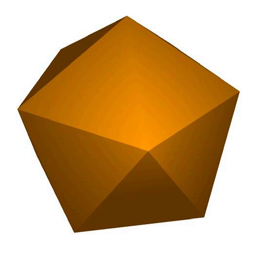
The icosphere shown has a radius of 1. The side is equal to 1.0515 units. This shape is sometimes used as the basis for subdivision in 3D modelling software and games.
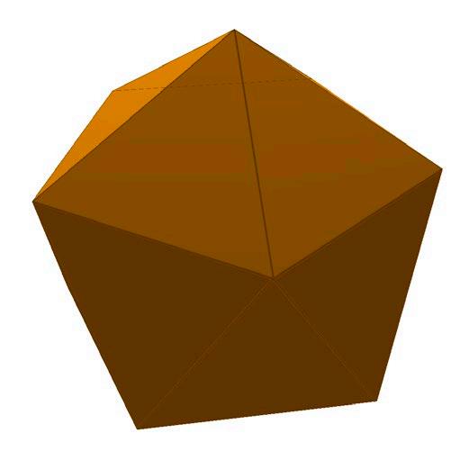
PROEFMATERIAAL©VANIN
There is a hidden element in this icosphere. Since the number of vertices is 12, it is possible to create three rectangles within the icosphere. These rectangles are perpendicular to each other, and what’s more, one side is s and the other side is determined by the golden ratio. There is always more to learn...
Chapter 9 The Icosahedron 221
PROEFMATERIAAL©VANIN
Chapter 9 The Icosahedron 222