Sulfuric Acid Manufacture Analysis control and optimization 2nd Edition Matt King
https://ebookname.com/product/sulfuric-acid-manufacture-analysiscontrol-and-optimization-2nd-edition-matt-king/ Financial Reporting and Analysis Using Financial Accounting Information 13th Edition Charles H. Gibson
Constructing IPRs When No Stabilized Tests Are Available 36
IPR Construction for Special Cases 37
Horizontal Welis 37
Waterflood Welis 37
Stratified Formations 38
Static Reservoir Pressure Unknown 39
Predicting Future IPRs for 011 Welis 40
Standing Method 40
Fetkovich Method 42
Combining Vogel and Fetkovich 42
Predicting Present Time IPRs for Gas Welis 43
Use of the Back Pressure Equation 43
Jones, Blount and Glaze Method 45
Predicting Future IPRs for Gas Wells 46
Weli Completlon Effects 47
Open Hole Completions 48
Perforated Completions 48
Perforated, Gravel-Packed Completions 53
Innow Performance Summary 54
Oil Welis ·54
Gas Welis 54
References 55
Introduction 57
Basic Equations and Concepts 58
The General Energy Equatlon 58
Single-Phase Flow 62
Two-Phase Flow 64
Two-Phase Flow Variables 64
Liquid Holdup 64
No-Slip Liquid Holdup 65
Denslty 65
Velocity 65
Viscosity 66
SUrface Tension 66
Modification of the Pressure Gradient Equation for Two-Phase Flow 66
Elevation Change 66
Friction Component 67
Acceleration Component 67
Two-Phase Flow Patterns 67
Pressure Traverse Calculation 67
Procedure When Temperature Distribution is Unknown 69
Fluid Property Calculations 72
Fluid Density 75
Gas 75
Oil 75
Waler 75
Fluid Velocity 76
Gas 76
Oil 76
Water 76
Empirical Fluid Property Correlalions 76
Gas Compressibility Factor 77
Salution or Dissolved Gas 78
Formation Volume Factor 79
Gas 79
Oil 79
Water 79
Isothermal Compressibilily 79
Viscosily 80
Oil 80
Waler 80
Gas 80
Interfacial Tension 81
Gas/Oil Inlerfacial Tension 81
GasN'laler Inlerfacial Tension 81
Predicling Flowing Temperatures 81
Flowing Temperature in Wells 82
Flowing Temperature in Pipelines 82
Well Flow CarrelaClons 83
PoeHmann a"d Carpenler 84
Hagedorn ane Brown Method 85
Duns and Ros Melhod 86
Orkiszewski 1'.lethod 86
Bubble Flow 87
Slug Flow 87
Transition Flow 87
Misl Flow 87
Aziz, Govier and Fogarasi Melhod 87
Chierici, Clucci and SclocchiMethod 88
Beggs and Brill Method 88
MONA, Asheim Method 90
Hasan and Kabir Method 90
Flow in Annuli 90
Hydraulic Radius Cancept 90
Cornish Methad 91
Evaluation al Correlations Using Field Data 91
Elfects 01 Variables on Well Performance 93
Liquid FlolV Rate 93
Gas/Liquid Ralio 93
Waler/OiI Ratio or Water Cut 94
Liquid Viscosity 95
Tubing Diameler and Slippage 95
Flow in Gas Wells 96
Flaw in Direclional Wells 97
Use 01 Prepared Pressure Traverse Curves 98
4
5
Preparation of Pressure Traverse Curves 98
Generalized Curves 98
Application of Traverse Curves 98
Pipeline Flow Correlations 104
Horizontal Flow Pattern Prediction 108
Eaton, et al., Method 109
Dukler, et al., Method 110
Seggs and Srill Method 111
Flanigan Method for Hilly Terrain 112
Hybrid Model 114
MONA, Asheim Method 114
Evaluation of Pipe Flow Correlations 114
Effects of Variables on Pipeline Performance 116
Liquid Flow Rate 116
Gas/Uquid Ratio 116
Water Cut 117
Liquid Viscosity 117
Pipe Oiameter 117
Single-phase Gas Flow 117
Use of Prepared Pressure Traverse Curves 118
Parallel or Looped Pipelines 122
Pressure Orop Through Restrictions 123
Surface Chokes 123
Gas Flow 123
Two-Phase Flow 124
Subsurface Safety Valves (SSSVs) 127
Gas Flow 127
Two-Phase Flow 127
Valves and Pipe Fittings 128
Eroslonal Velocity 129
References 129
Total System Analysis 133
Introduction 133
Tubing Size Selection 135
Flowline Size Effect 136
Effect of Stimulation 139
Systems Analysis for Wells with Restrictions 141 Surface Chokes 141
Subsurface Safety Valves 143
Evaluating Completion Effects 143
Nodal Analysis of Injection Wells 146
Effect of Oepletion 148
Relating Performance to Time 150
Analyzing Multiwell Systems 151
Artificial Lift Design 155
Introduction 155
Continuous Flow Gas Uf! 155
Well Performance 156
Valve Spacing 160
Gas Uf! Valve Performance 165
Otis Design Procedure 167
Submersible Pump Selection 174
Sucker Rodor Beam Pumping 177
Hydraulic Pumping 183
Summary 183
References 185
Nomenclature
Appendix A
Two-phase Flow Correlation Examples Hagedorn and Brown Method 191
Appendix B
Pressure Traverse Curves 197
INTRODUCTION
-\ny procluctioll \Vell drillcd :lnd completcd lo mQVC (;-:(' oil Ol" fnJl1l irs original iocatioll in the rescrvoir
¡he stock tank or sales line. or {rampart of ¡:-,¡;';C !luids rcquircs to t)V('rcol11c friction losscs ::1 Ihe syslcm and lO !in (he products to lhe surfJcc. The (uids mus! travel Ihrough rhe rescrvoir and lhe piping and ultinltHe]y 110\\1 into J scparator for gas-liquid
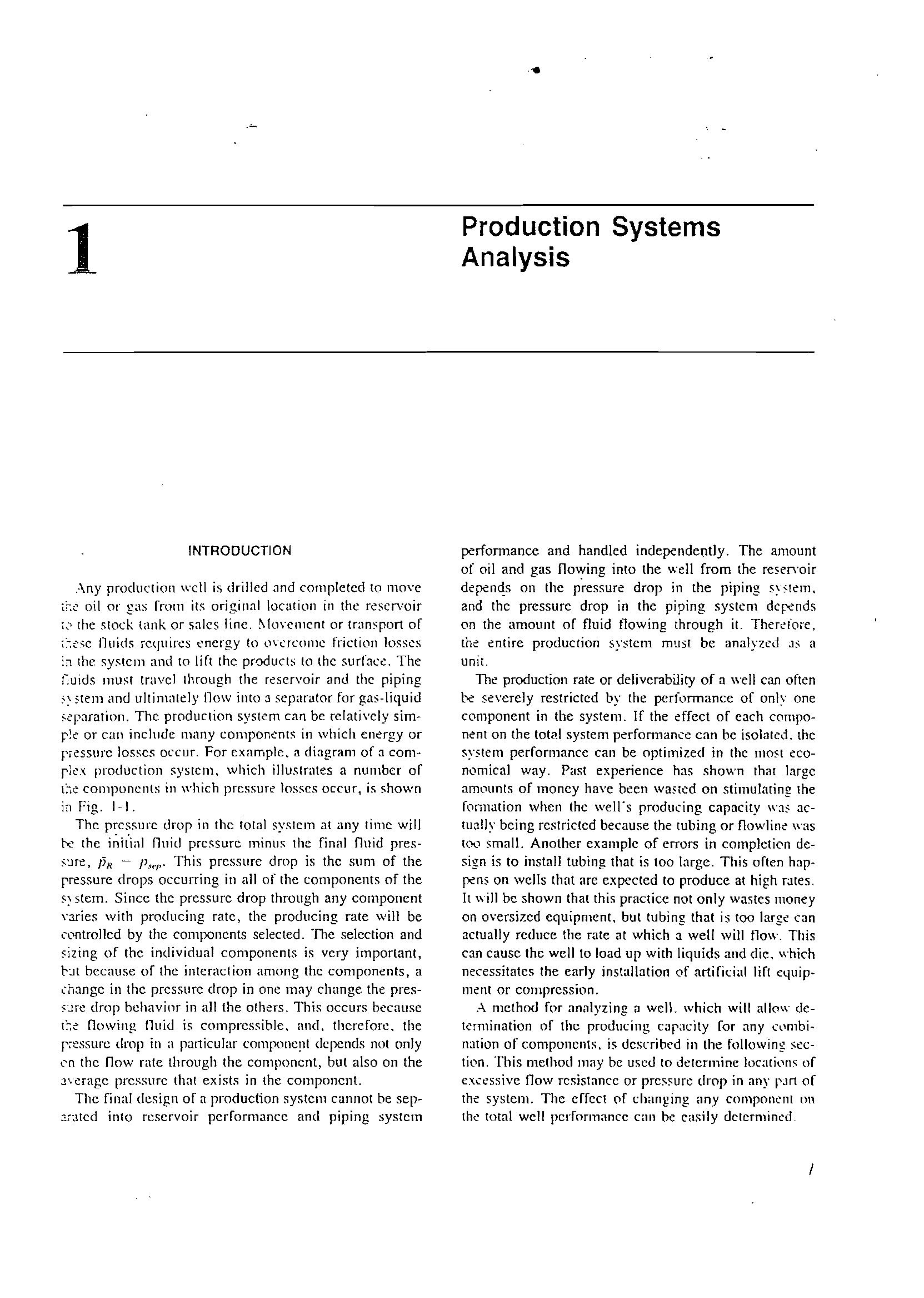
Thc produclion system can be relati"cly simr!c or can ínelude many components in which energy al' fíessurc losscs occur. Far cxample. íl diagram of:1 COI11rkx production systcm, which ¡Ilustrares a numbcr of l:-;e componcnls in which prcssure los ses OCCUf, is shown ioFig.I·1.
Thc prcssurc drop in thc fotal syslcm al any lime will the iñitial nllid prc!'surc minus Ihe final nuid prespI{ P ",. This pressure drnp is the slIm of the rressure drops occurring in all ol' lhe componcnts of the stem. Since the pressure drop through any component yaries with producing rate, the producing rate will be cQntroJled by Ihe components selecled. The selcction and of the individual components is very important, r:Jt because of Ihe intcraction í.lmong the components, a ch.:lIlge in the prcssurc drop in one Il1<lY change the pres:,"Jre drop bchavinr in all the others. This occurs because Oowing !luid is compressiblc. amI. thercfore. the drop in a pal1icuJar componcpt dcpcnds not only en the now rate through the component, bUI also on the J\'aage pressure lhat exists in lhe componcnt.
Thc final dcsign of a production syslel1l cunnot be sep2í3tcd into rcservoir performance amI piping .systell1
Production Systems Analysis
perfonnance and handled independenlly. The amollnl ol' oil and gas inlo the \\'ell fram the reservoir depen,-!s on the pressure drap in the piping sY:'lem and the pressurc drap in the piping system dq:-ends on the amount of fluid tlowing through il. Ther-=,iore, the t:nlire production system mus[ be analyzcd J:; a unir.
The production rale ar delivcrability of a \\'ell can aften be sevcrely restricted by the perfonnancc of on!y one component in the system. If the effcct of cach component on Ihe tot<'l.1 system perfannance can be isoIalcd. the systern performance can be optimized in the rnost economical way. Past experience has sho\\'n thtH Jarge amounts of moncy have been wasled on stimulating lhe [onnation when the we¡¡-s producing capacily \\'3:' acrually bcing restricted because the mbing or Oowline was [,-X, smal!. Another cX3mplc of errors in completiC'n design is to install tubing that is too largc. This often happen, on wells Ihat are expected to produce at high rales. lt will be shown thar this practicc not only was[es Illoney on oversized equipmcnt. bUI tubing that is too large ('an actually reduce the rate at which a well will no\\'. This can cause the wcll to load up with liquids and dic. which ncccssitatcs lhe early ínst.tllation of artifici.tl lift menl or comprcssion.
A mcthou for analyzing a wel1. which will alk'!\\' dck'mlination of the producillg c;:IracJty for any C'llmbin:ltion of componcnts, is desnibed in lhe following st::ction. This melhod may be uscu (o delcnninc locafit1rts of c.\(:essive Oow rcsislance or drop in any of the systcm. Thc crfcct of changing <lny componl'nt on th<' total wcll performance can be easily dclcrmincd,
AP4 = A Ps c> P6 = c> P7 c> PB = I t. P, =(Pw's - Pw,)--1 ....------1 A P, =(PFi - Pw's)
Fig. 1-1. Possible pressure losses in complete system.
SYSTEMS ANAL YSIS APPROACH
Pwh-Psep t.p, t.P2
Pusv-Posv
Pwh -PDse
POSC-Psep
Pwf-Pwh
LOSS IN POROUS MEDIUM LOSS ACROSS COMPLETION " "RESTRICTION " SAFETY VALVE SURFACE CHOKE IN FLOWlINE
TOTAL LOSS IN TUBING " FLOWlINE
The systems analysis approach, oflen caHcd NGDAL '" Analysis, '" has becn applied for many years to analyze the perfonnance of systems eomposed of interacting eomponents. Electrical circuits. complex pipeline networks and centrifuga! pumping systems are a11 analyzed using mis method. lts applicadon to well producing syslems was firsl proposed by Gilbert' in 1954 and discussed by Nind' in 1964 and Brown' in 1978.
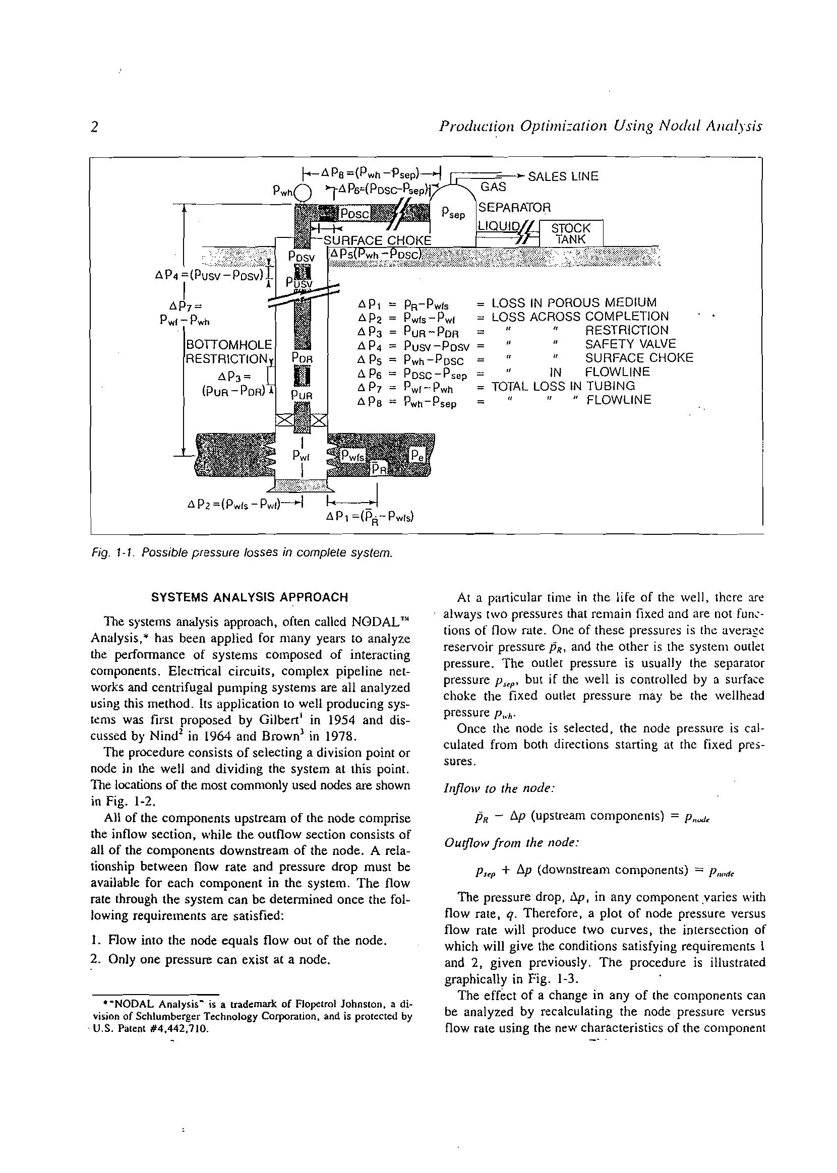
The procedure consists of selecting a division poiot or node in lhe well and dividing the syslem al lhis point. The locations of lhe most commoruy used nodes are shown in Fig. 1-2.
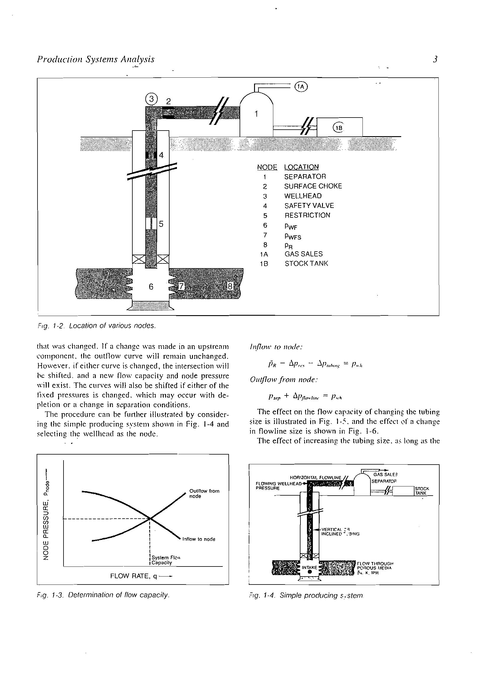
AH of the components upstream of (he nade comprise (he inflow section. while the ou(f1ow section consists af all of lbe componenLS downstream of the node. A relationship between fiow cate and pressure drop must be availabJe foc each component in the system. The flow rale lhrough lhe system can be delermined once the following requirements are satisfied:
1. Flow inlo lhe node equals flow out nf lhe node.
2. Ooly one pressure can exist at a nade.
·"NODAL Analysis" is a uademark oC Flopetrol JohnSlon, a di8 'IisiDn oC Schlumberger Technology Corporation, and is proteeted by U.S. Palent #4,442,710.
At a particular time in the Efe af (he well. there are always [wo pressures !.ha( remain flxed and are not fun.:tioos of ilow rateo Ofie of these is (he aver.lge reservoir pressure PRI and (he other is the s)lstem audet pressure. The outlet pressure is usually (he separaror pressure Pup' bU[ if the well is cOnlrolled by a surface choke the fixed oullet pressure may be the wellhead pressure P IJ.
Once the nade is selected. the nade pressllre is calculated from both dírections starting at [he fixed pressures.
inj10w fo the node:
fiR - t:.p (upstream componen!s) = P"..J<
Outflow from the lIode:
PUP + l1p (downstream eomponents) ::::: P""dc
The pressure drop, IIp, in any component ,varies wilh flow rale, q. Therefore. a pJot of nade pressure versus flow rate will produce two curves, the intersection of which will give the canditions satisfying requiremenlS 1 and 2, given previously. The procedure is illustrated graphically in Fig. 1-3.
The effect of a change in any of the eomponents can be analyzed by recalculating the nade pressure versus flow rate using the new characteristics of the componenl
LOCATION
SEPARATOR
SURFACE CHOKE
WELLHEAD
SAFETY VALVE
RESTRICnON
PWF
PWFS
PR
GAS SALES STOCKTANK
,e,g. 1-2. Localion 01 various nades.
rhat waS changed. Ir u changc was made in <lO UpSlrC<l1ll (oll1poncnt. lhe Gutllo\\' curve wil1 rCI1l3in unchanged. Ho"ve er. if cithcr curve is chang:cd, lhe intersection \ViII Pt: shifteu. and a IlCW !lo\\' capadty and node pressure \\'¡II cxist. Thc CtlfVCS \ViII also be shifted if eithcr of the fixcd prcssures is changcd. which may occur with depletion or a chunge in separatioll conditions.
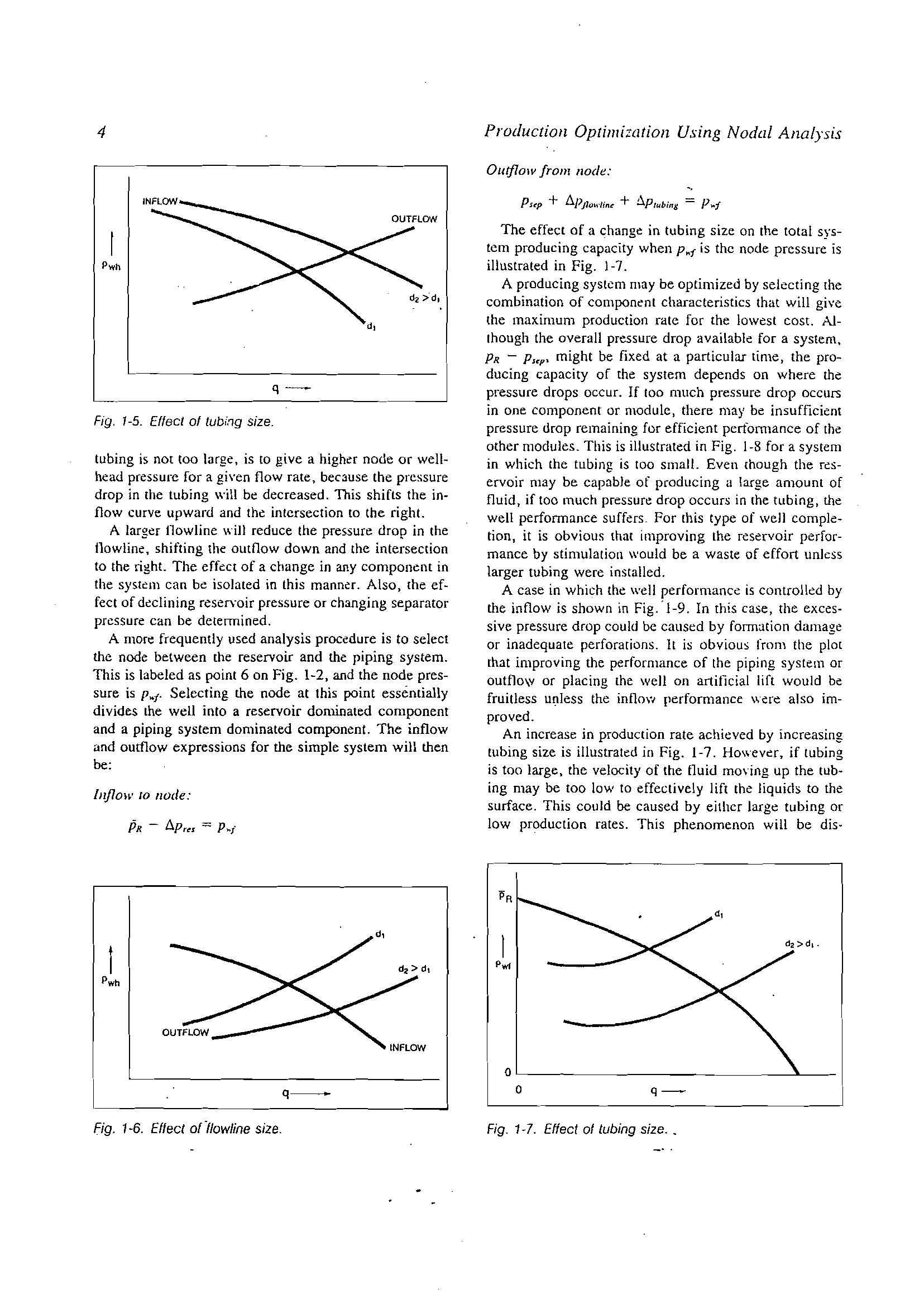
The procedurc can be furthcr illustrnted by considcring the simple producing systcm shown in Fig. 1-4 3nd the wellhcad as ¡he nade.
I ro Hode:
Qutj70w from nade:
The effect on the flow capxity of changing. the tubing size is illustrated in Fig. 1-:'. and thc crfce! l.."'If <1 dwnge in flowline size is shown in Fig. 1-6.
The effcct of increasing: thc tubing sizc. :.1:' long as the
,C¡g. 1-3. Oeterminalion o( ffow capacity.
1-4. Simple producing s.'stem
tubing i5 not too large, is to give a higha node or wellhead pressure ror a gi\'cn flow rate, bec3use the prc.ssure drop in [he tubíng wiB be decreased. This shifts the ioflow curve upward and lhe intcrsection te the right.
A lar'2.er tlowline will reduce {he pressure drop in (he shifting the outtlow down and (he ¡ntceseerian to the right. The erfeer of a change in any component in {he system can be isolarcd in lhis manoa. Also, {he feet of declining reseryoir pressure or changing separator prcssure can be determined.
A more frequently used analysis procedure is to select (he node betwecn (he reservoir and me piping system. lllis is labeled as paint 6 on Fig. 1-2, and lhe nade pres5Ufe is P f' Selecting the node at Ihis point esséntially divides lhe well ioto a reservoir dominated eomponent aod a pipiog system dominated eomponenL The inflow and outf1ow expressions for the simple system will theo be:
Inflon' 10 nade:
Productioa Optimizalioa Using Nodal Analysis
OUtflOIV from node:
Pup + !J.Pllwli.< + :'J.p,",;., = P-t
The effect of a change in tubing size 00 the total systcm producing eapacity when P f ¡s the node pressure is illustrated in Fig.
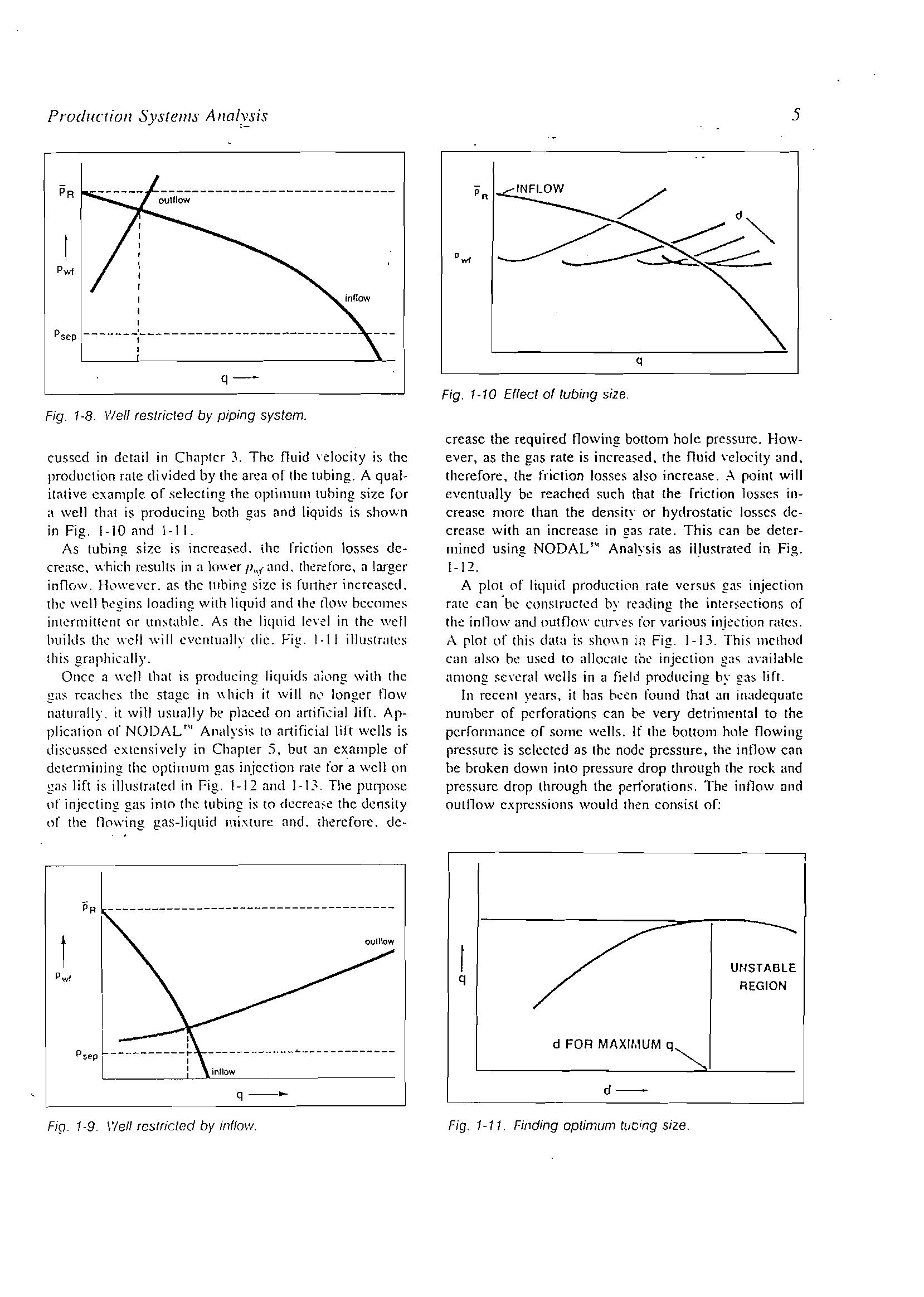
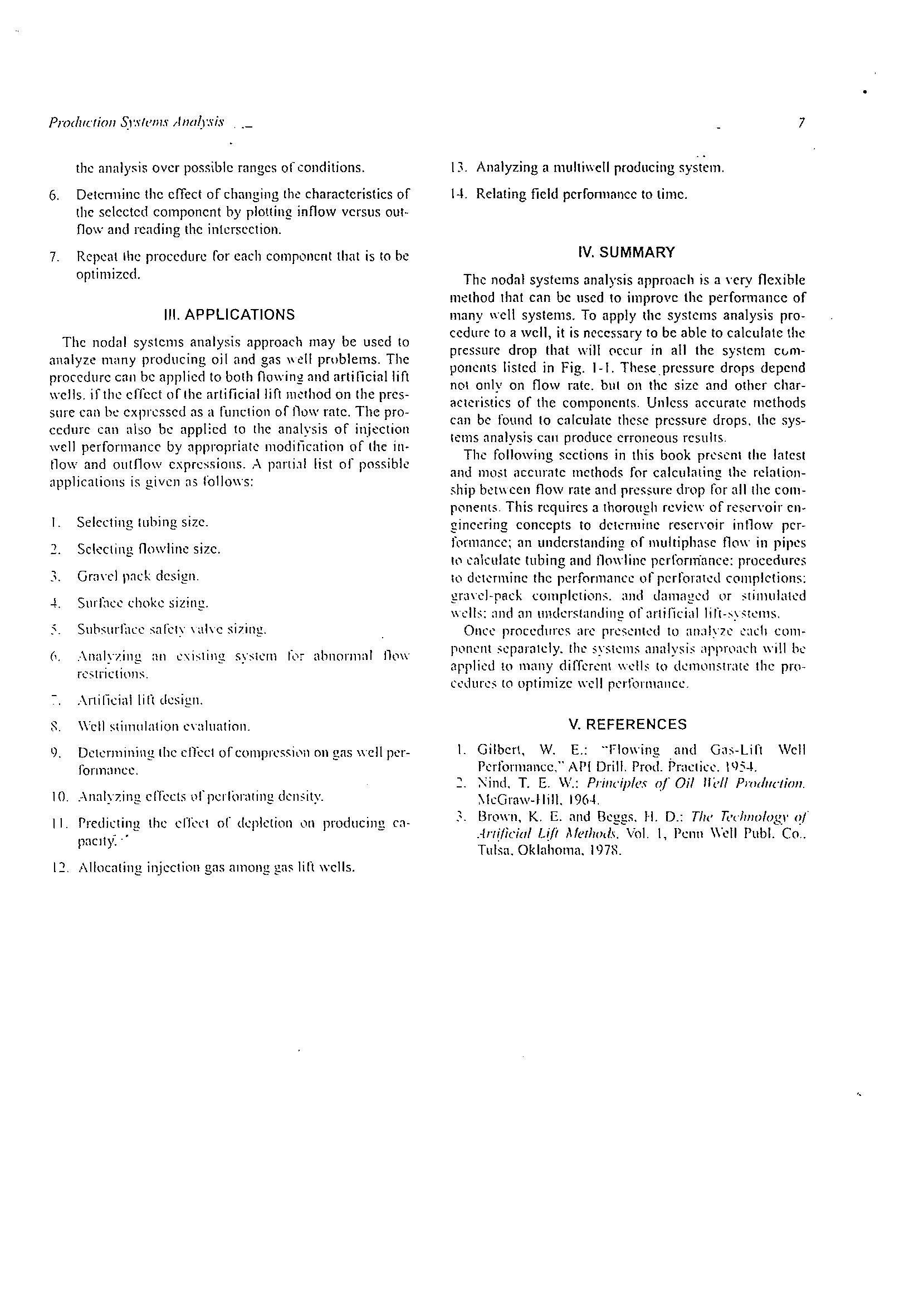
A producing systcm may be optimized by selceting {he eombination of component characteristics that will give the maximum production rate foc {he lowest cost. Although the overall pressure drop available for a system, PR - PUP' might be fixed at a particular time, the producing capacity of rhe system depends 00 where the pressure drops occur. If too mueh pressure drop occurs in one component or module, there may be insufficiem pressure drop remaining for efficicnt perfornlance of the other modules.This is illustrated in Fig. 1-8 for a system in which (he tubing is too slllal!. Even [hough the reservoir may be capnbJe of praducing a large amounl of fluid, if too much pressure drop occurs in (he tubing, the well perfonnance suffers_ For this eype of \Vell eompletion, it is obvious (ha¡ improving the reservoir performance by stimulation \\'ould be a waste of effort unkss larger tubing were installed.
A case in which the well performance is controlkd by the inflow is shown in Fig.·1-9. In rhis case, the exccssive pressure drop could be caused by fOITn<leion damage or inadequate perforarions. II is obvious from tlle plor [hat improving the performance of the piping system or outflo\V or placing lhe weH on artitlcial !ift would be fruitless the inflo performance were a150 irnproved.
An increase in produclion rate achieved by íncreasing tubing size is iIlustrated in Fig. 1-7. Howevcr, if lubing is too large, the velocity of (he fluid moving up the tubing may be too low lo effectively ¡ift the ¡iquicls lo the surface. This could be caused by either large tubing or 10w production rates. This phenomenon will be dis-
Fig. 1-5. Ellecl 01 lub{ng size.
Fig. 1-6. Ellecl oOlowline size.
Fig. 1-7. Elfect 01 lubing size
q
Fig. 1-8. \.'Iell res/rieled by plping sys/em.
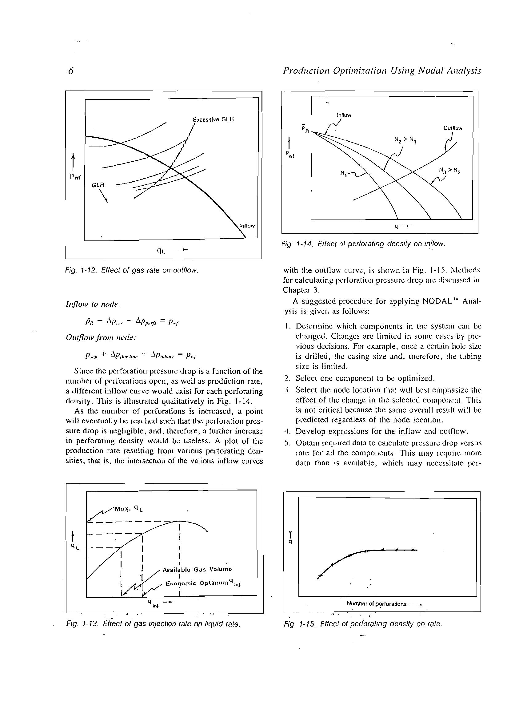
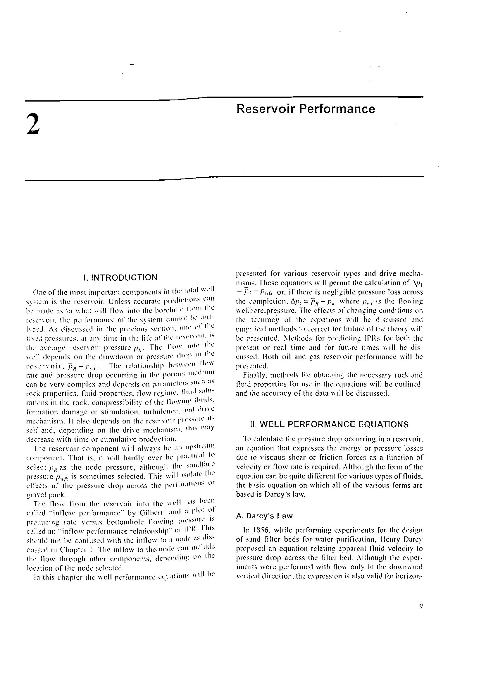
cusscd in dctail in Chaptn J. Thc nuid \'eloeity is the produClion rate divided by lhe area of lile lubing. A itative cxample of selccting lhe optimu11l tubing size ror a well is producing both gas <lnd liquids is shown in Fig. 1-10 and 1-11.
As tubing sizc is increased. ¡he frictiL'1l losses dccrt:<lSC, which results in a lower ¡J"f ando rherdorc, ti larger innow. H<Jwevcr. as rhe ltIhlng sizc is runher ¡ncreaset!. the wcll hegins loading with liquid ami rlo\\' bccoll1cS inlamittent nr unst'lhle. As lhe liquid k\'el in lhe \\'el1 huilds Ihe \\"ell will c"cntllally die. Fig. 1·11 illustratcs Ihis graphically.
Once a \\'ell lhat is producing liqllids ail10g wiril [he ga;; rcaches Ihe stagc in \\'hich it \Vil! longer tlow natur<llly, it \ViII usunlly be 0/1 artificial lin. Applicalion (lf NüDAL TI1 Allillysis to artificial lin wells is dis('usscd cxlcnsivcly in Chapter 5, bu! :ln example of dctermining (he optimulll gas injcction rale for a wcll on gns lirt is illustratcd in Fig. 1-12 nnd 1-13. The of injccling gas inlo the tubing is to dccrea:,e the dcnsity nI' the tl(lwing gas-liquid mi.\tllTc amI. ¡hercfore.
crease the required tlawing ballom hale pressure. Hawever, as the gns rate is incrcas.ed, lhe nuid \'clocity and, lherefore, !'rictian lasses alsa ¡nerease. A paint \ViII cvcntually be reached that the frictian losscs ¡ncrense more lhan the density or hydrostatic losscs dccrease with an ¡ncrease in gas rate. This can be dctcrmincd using NODAL n, Analysis as ilIustrared in Fig. 1-12.
A plot of liquid productil11l rale vcrSU5 gas injection rate can <be cOllslructed by rCJding the interscctians of the inllow anJ oUIOo\\, cur\'es for various injection rates. A plot of (his is shown in Fig:, 1-1 J. This mClhod can also uscd lo allo('n[c ¡he injection J\'íúlahle among wells in a field producing by gas lin. In recent years. it has becn found th3t Jn inadcquntc numbcr of perforations can be very dctrimenta! to the performance of SOIllC wells. lf Ihe boltom hl)le flowing pressurc is selecled as the node pressure, rhe inrlow can be broken clown iota pressure drop through the rack and prcssurc drop through the perfarations. The inllaw i:md outtlow cxprcssions would lhen consist of:
UNSTABLE REGION
Fig. 1-10 Efleel 01 lubing size.
Fip. 1-9 l'lelf rcsfricled by inf!ow.
Fig. 1-11. Finding optimum tucing size.
IllfloU' lO /Jode:
OU{/7ow ¡ro", Ilode:
Since ¡he perforation pressure drop is a function of the number of perforations open, as well as prodüction rate, a different ¡nnow curve would exisl [or each perforating density. This is illuslraled qualitatively in Fig. 1-14.
As [he numba of perforations is increased. a point will eventually be rcached such (hat the perforation pressure drop is ncgligible, and, therefore, a further ¡necease in perforating density would be useless. A pIar of the production rate resulting from various perforating densities, that ¡s, lhe intersection af the various inflow curves
with the autflo\\' curve, i5 shown in Fig. 1-15. ror calculating perforation pressure drop discusscd in ehapler 3.
A suggested procedure for applying NüDAL '" Analysis is given as follows:
l. Determine which eomponents in (he system can be changed. Changes are limitcd in some cases by previous decisions. For example, once a cert:lin hale sizc is drilled, the casing size and, thcrclorc, (he tubing size is limited.
2. Select ane component lo be optinlized.
3. Select lhe node location thar will bes! emphasize (he effeet of the change in lhe selectcd componcnt. This is nol critica1 because lhe same ovcrall resuh will be predicted regardless of the node localion.
4. Dcvelop expressions ror the infiow and oulOow.
5. Obtain required data to calculare prcssure drop versus rate ror aH [he components. This may require more dara than is available, which may necessitate per-
l'l/Iow
Fig. 1-14. Elleel o/ per/orating densily en inflow.
Fig. 1-12. Efleel 01 gas rale on outflow.
Fig. 1-13. Efleet 01 gas injeclion rate en liquid rate. Fig. 1-15. Elfect 01 perlori!ting density on rate.
Producriol1 S.1'",rems
the <!nalysis over possiblc ranges of conditions.
6. Oelenninc lhe cITect of ehanging (he characteristics of ¡he selcctcd eomponent by plotting innow versus now alld reading lhe intcrscctioll.
7. Repeallhc proccdurc ror ench component tlwt is to be optimizcd.
111. APPLlCATIONS
The nodal systcms analysis approach may be uscd to <In<llyzc m¡my producing oil and gas \,e1! pmblems. The proccdure C<lll be applicd to bo!h Oowing tlnd artificiallift wells. ifthe ef(cet ofllle arlificiallift lllClhod 011 the pres5ure cnn be cxprcssed as a fUllelion of Ilo", ratc. The proccdure can also be appl:cd to the analysis of injection \vell performance by <lppropriate llloditicatic)Jl of Ihe intlo\\' and oufflow o:pressiol1s. ,-\ pani.11 li5t 01' possiblc applications is givell as follo\Ys:
Thc nodal systcms analysis approach is a \'cry ncxihlc melhod that can be uscd to impro\'c lhe perfonmlllcc of many "'el\ systems. To apply Ihe systcl11s analysis proccdure to a \Vell, it is nrCeS:':i3ry to be ablc to calculnlc thc prcssure drop tl13t wiJl (lCcur in al1 the sy:-Iem CL.nlponcl1ts listed in Fig. 1-1. These. prcssure drops depcnd not only on now mte. bUI on the sizc and other charaCleristics of Ihe eomponents. Un1css accuratc Illcthods can be fOUlld to cnlculalC thcse prcs:-ure drops. lhe systems analysis can produce crrOllcous rcslllts.
The following sections in this book prcscnt Ihe l<1tcsl and Illost accurate 111cthods for calculating lhe rci::lliollship bctwcen now rnte ane! pressure drop fol' <111 Ihe COI11p0nelHs. This rcquircs a thorough rcvicw of rescr\'oir ginecring concepts to dClcrmine rescn'oir intlow pcran underslanding of nO\\' in pipes 1(" ca1culatc tubing and nowlillc pcrlorm'ance: procedures Il) dct12'rminc the performance 01' CClll1plctiol1s: t:olllplcriol1s. ami damelgcd or :,til1l11lal12'd \Yell:,: :llld <111 undcrs(andillg ofartil1ciallil'¡":'Y.:;(L'llls.
Once procedures are presclllcd to an:llY7c C0111pl1!lelH :'eparalely. Ihe sys!e1l1S allillY'sis :lpprl)adl will be applicd lo many dilTcren\ \\'ells (o dCl11l)J1stratc Ihe proccdurc:, to optimize "'cl! performance,
V. REFERENCES
1. Gilbcrt, W. E.: "Flowing and G,b-Lirt \Vell Performance," API Drill. Prod. i'raclicc. \ 95-J.. :\ind. T. E. W.: Pril/ciples (?( Gil IIdl ProdUcliol1. 'IcGraw-f1ilJ.
Bro\\'n, K. E. tl!ld Beggs. H. D.: rhe Ti:cllllology .irr(/icia{ '\/er¡'od\. Vol. 1, Pelln \\'ell Publ. Co .. Tuls<1. Okl<1homa. 197fl.
1. INTRODUCTION
Oile of thc illlJ10rlrllll componenl:, i'n llll' 1\11;11 \\"cll is Ihe Ulllc:,s tlCCllr;J{C pn'dil'tl\Il\:' l':1I1 t;l' :,l:1dc \0 \\ lut will I1tH\ ¡nltl ¡he lltlrt'llt11t' 1"("111 ¡!lL' rC':';:;-\L,ir. Ihe pcrl'llrll1¡lllCC (Ir {he Systclll (';1(lfln! l·,' ,111;1h ;:;:J. As disCllS:,cd in lhe prC\"i0US s,xlinll. IJlI" ,>1 111\ ' pn:ssu["c:-,. ¡JI :lllY lil1lc in ¡he 1ire l,ftlll' 11",\'1\,'11. IS 111;: J\'cragL' rcscr\ nir prcssurc Ji". T11I..' 1111\\" l111t' 1111..' \\(':', dcpcnds 011 lhe dra\\"(1L1\\"Il or prl..'Ssun.: 111111' 111 lh\.' />R -/\". The rclati\lIlship b\'I\\",11 1!l1\\" prcssurc drop occurring in Ihe ptlrtlll" 111,\1111111 cm be vcry cOlllpkx and dcpcnds 011 parallll'lL'IS :--11,-11 as propcrtics. !luid propcrtics. !lo\\' !"l',t:.illll'. I1l1hl in IhE: rack. comprcssibility 01' Ihe 1l11WIII!: llllllb. ft1¡-::wtion dam<lcc nI' stimulatioll. lurhu1clll'l', ;,,111 ,hwe ll1.:.::nanisl11. It al:'(l dcpcnds on lhe rcs('r\'t1lr ¡Ise1;' and, dcpcnding 011 lhe dri"c 1\1:1)' dcccasc \\'¡Ol limc nI' cUll1Ulalivc produClitlll. Thc rcsen'oir c\llllponcnl will ah\"ay:-: \w ;111 cllmpOncnl. That is. it will hnrdly cver he lo PR as the Ilodc prcssurc, although Ihe prc":,surc Pub is sOllletimcs selccted. This \\'ill ISI1!:lh' [he ctl'c,,:ts of ihc prcsslIrc drop <leross the !Wrl"nl:1Ih,n:-: tlr gr3\"el pack.
The no\\' frolll thc reselToir inlO the \\"l'1I 11:\:-: bl'1..'1l C;1:)('l! "inflo\\' performance" by Gilb('rl ' alld ;\ phI! t.lr pr\'..lucing ¡'<lle \,('rSU:-i botlo11lho1c clL'd ílll "inflo\\" performallce rc!aliollsl1ip" (}I 11'1' :,lh'·.ild nol b(' cOllfuscd wilh Ihe ínllo\\" [I};l 11l11k :1:' dlSin Charter l. The in!low to l!le. node l':lll fhe !low Ihrollgh oll1el" eomponellls. \'11 lhe of the IlDlk selccted. !;] this chílplcr Ihe \\'el! pcrform:111cc eqll:llillll ..; \\ dI be
Reservoir Performance
prc:,('nted for various types and drive I1lcehanisll1:'. Thcse equtl\iOll5 \\"ill pcnnit Ihe calculation of J.Pt :::: ro: - or. if Ihero:;- is negligiblc prcssure 105s across the ÓI'I = P.I? -1'". where Pu'- is the ll(l\\'ing The I.:'ffl.:'c\:' ch:lllging conditit111s (In the ::..:'cllfncY 01' Ihe cqualil1 n:, ",jI[ be disclIsscd :llld lo (\lrrc'(l fN failurc nI' {he lhenry \\-il1 be \lclhods rOl' prt'Jieling IPRs rnr l1lllh Ihe IWC5;,';lt 01' re<ll timc <llld for tlllun.' times "'ill be l30th oil tlnd g:lS rcsl'f\l)ir pl'rformancc \\"ill he ¡m::'(':l1cd.
Fi¡ully, mcthods for obtaining the nccessary roc.k and fluid rropcrties rOl' use in the equatiolls \\'ill be ollllincí.l, ane. ¡he accuracy of the data \\-ill be disCllsscd.
11. WELL PERFORMANCE EQUATIONS
T\' ..:::tlctdate the prcssure tiror occurring in a ITsc[\·oir. all ;,'..:juation that cxpresscs the cncrgy al' prcssurc losscs du\:' w viscous shcar or frictit'!n forces as a funclion al' ve!L'..::ily al' f10\V rate is requircd. :\1though lhe form ofthc can be quite difierenl for various typcs offluids, the [,Js.ic cqllation on which all of lhc variolls form5 are is Darcy's law.
A. Darcy's Law
Ir. 1856, whilc pcrforming for {he dL'sig.n of s.md filler beds for \\'alcr purifi(',ltion, Ileury Dan:y pmrl':,ed an cquatioll rclating arparcll! lluid vclocily lo prc:,:,urc drop aeross Ihe filter bed . .\ithough the c.\pcr\\'crc performcd with tlll\\' only in the dO\\"ll\\"ard veni.:al dircction, the c.\prcssi011 is abo val id ror horizoll-
tal flow, which is of mast ¡nterest in lhe pctroleum industry.
It should al so be noted that Darcy's experiments involved only one Huid, water. and that the sand [¡{ter was completcly saturated with the water. Thercfore, no effccts of fluid properties oc saturation were involved.
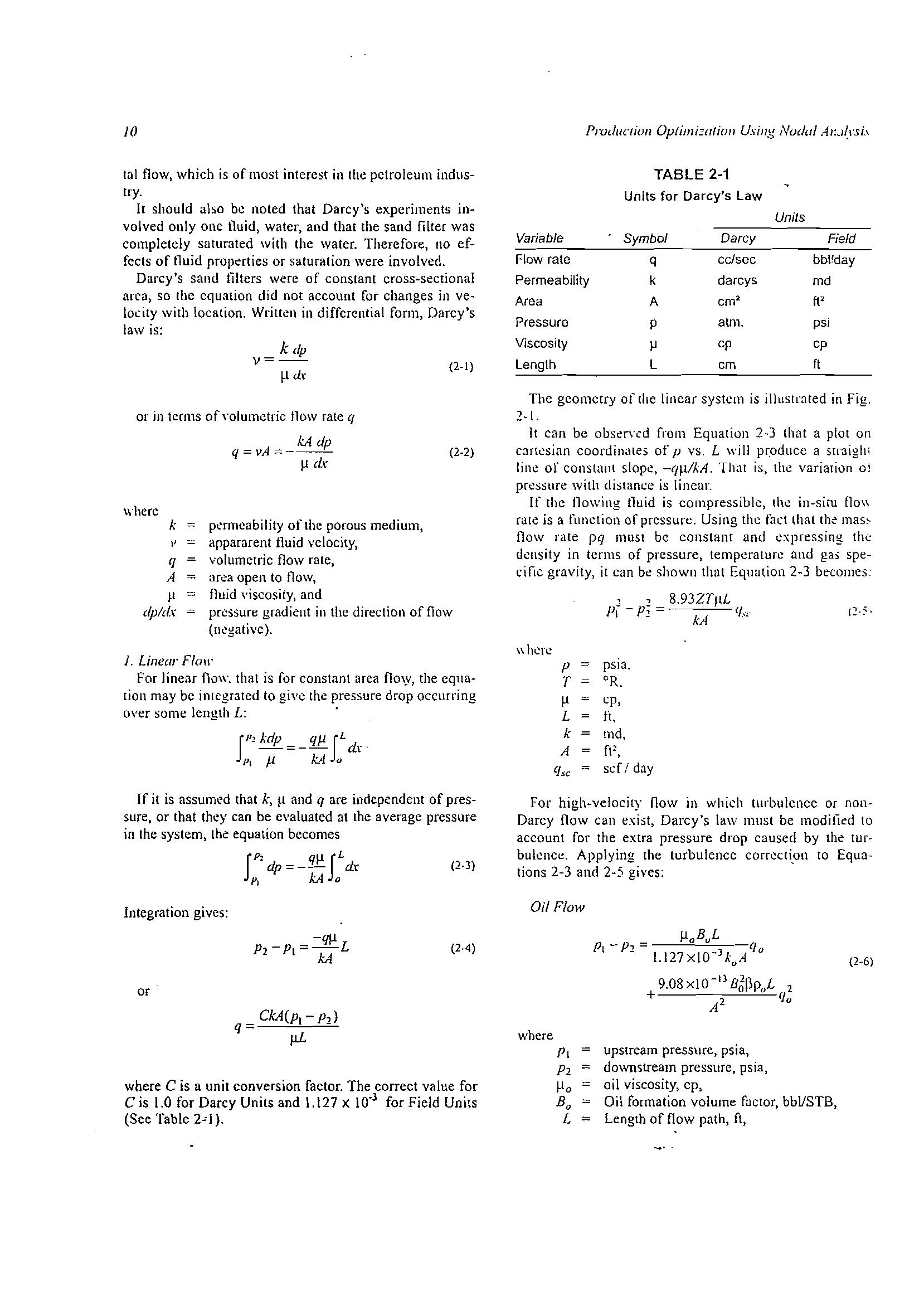
Darcy's sand tilters wece of constan! cross-sectional arca, so lhe cquation did nol account roc changes in vcwith localion. Writtcn in diffcrentiai form, Darcy's law is:
kdp v=-!l ti,
wherc or in tcrms oh'olumctric now rate q
q = vA =_ kA dI' !l el,
(2-1)
(2-2)
PJVdUClioll Oplimizalioll UsiJlg Nudul
TABLE 2-1
Units for Darcy's Law
Units
Variable Symbol Darey Field
Flow rate q cc/sec bbl'day
PermeabHity k darcys md
Area A cm' ft'
Pressure p almo psi
Viscosity cp cp
Lenglh L cm ft
Thc gcol1lctry of ¡he linear systclll is illllstr[\ted in Fig. l.
It can be obsaycd from Eguatían lhat a plot on coordillJleS of p vs. L \ViII pr.oduce a srr¡:üglli line of constanl -qW'kA. TIJat is, the variarion al pressure with distance is linear.
If the nowing tluid is compressiblc, lhe in-siru 00\\ rate is a fUl1ctiol1 01' pressure. Using the t:1et lhal lhe now rate pq mus! be constant and the dClIsity in tcnns of prcssure, temperatun: and ga:i specinc gravity, it can be showll thut Equation 2-3 be-comcs' k v = q A P dpld,
J. Linear Flol\"
pc.:-rrncability oflhe paraus medium, appararcnt fluid vclocity, volurnctric flow rale, afta open lo now, fluid viscosity, and pressure gradient in lhe direclion of flow (llL'gati\'c). , , 8.93ZT¡tL JI, - Pi kA '/."
For linear now. that is [or constant area flO\y, the cquation may be intcgratcd to gívc the pressure drop occurring Qver some Icngth L:
JP' kdp qJ1 fL -=-- el, PI J.l kA o l' T ft L k A pSIJ. °R. ep, ti, md, fe, scf / day
(2·:'
If it is that k, and q are independent of pressure, or that they can be cvaluated at lhe average pressure in the system, the equation bccomes JP' qp JL -dp=-- elr PI kA o
Integration givcs:
(2·3)
where e is a unit conversioo factor. The correet value for e is 1.0 for Darcy Units and 1.127 X 10⁻³ for Field Units (See Table 2"1). or q -q¡.¡ p,-Pt =--L kA
CkA(p,- 1',) J1L
FOl" high-velocity f10w in which turbulcnce or 0011Darcy Oow can exist, Darcy's la\\' must be moditied lo accaunl for the extra pressure drop cJused by the tUfApplying [he turbulencc corrccti,on to Equatians 2-3 and 2-5 givcs:
Oil Flow
(2-4) where 1', 1', !lo Bo L upstream pressure, psia, do\,·mstream pressurc, psia, oil viscosity, cp, üil fonnation volume f"ctor, bbl/STB, Length of flow path, n,
(2-6)
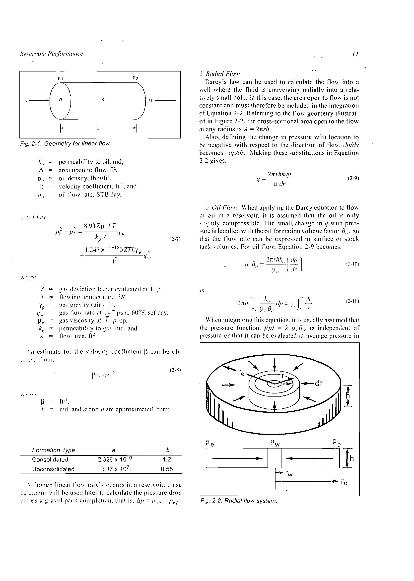
F"f;. 2-1. Geometry for linear tlo','/.
J. Radial FIOlI'
Darcy's law be us.cd to calculatc the no\\" into a \,"eH whcrc lhe fluid is convcrging radially into a rclati,"cly small hale. In this cnsc, Ihe arca open lo now is nat constnnt amI mllst ¡herefare be included in lhe integrntion 01' Equation 2-2. Rdcrring lo Ihe no\\" geomclry iIIustratcd in Figure 2-2. the apcn lo lhe now any radius is A = 2Itr" -\150, dcfining the changc in prcssure wilh localion to be negalivc \Vith rcspcct lo lhe dircction of no\\". dl'ldr becomcs -dpldr. thcsc substitutions in Equatioll 2-2 gives:
lío pcnncability to oil. md, A arC<l open lo Ilo\\". n=. Po oi! dcnsity. IbnlitV. \"Clocily coclliciClll. n-l. and (1" =-: oil llo\\' raleo STB day. 2¡rrhkd[J q:::o ' dI' 12-9)
l;.' FIfJ\\" : '2 I't -P::::: Cjg kg.1
1.247 xl ,)-J('PZTLy " , + q: r (2-7)
g'IZ dL'\i'llillll 1.,'\'1111:llct! ;11 T. .!'.
J1l)\\ing [l'mpl.'ra:::r;.'. 1?
g;l:, gr:n'ity : J.
gil:' 111..1\\ rate ¡It :,:. - psi<t 6tY'F. sef day.
ga:, \'iscosity a( T. ¡J. ep. 10 md, <llld
.:, Oil Flan: \\·hcl1 applying the Darcy cqualion lO !lo"," \)f ,,1jl in a il is that lhe oil is only :-li-;¡Hiy comprcssiblc. lile small, changc in q wilh prcsi::; halllllcd with lhe oil fOrlllJ::ion "olume factor B", so Ihe Ilo\\" rate can be cxprcs5cd in surnlce llr stock ud: '"olullle:-i. For oil Oo\\', EqUJlion 2-9 b,,:coll1c::;:
\n cstimatc Ihe ClldliciCll! [3 Clll be ob";:d rrom:
\\"h ll inlegraling: cqutllioll. it i:-; assulllcd that lh,:- prcssurc rUIlClioll .tfl'J oc:: k P.,B,. is indcp('ndcnt ('Ir or lhílt il ":-tln be al avcrngc prc""urc in
md. and a and b 3fC approximalcd ¡'rom: P k Formation Type
Consolidtlled
Uncorlsolidaled
\llhough lincar !lo\\' rafe!y L1ccurs in tl n,::sL'r\-t1ir, Ihese .:Jtinlls ",ill be llscd blter 1\1 .:,\!culalc lhe drop ;1 pack COlllplcli,,111. Ihal i:-;. ófJ = / 1 ,,; - pur. F;), 2-2" Rad;aJ (fow sys{em. 1.2 0.55 b 2.329 X 10 10 1.J7 X 107 , a fr'.
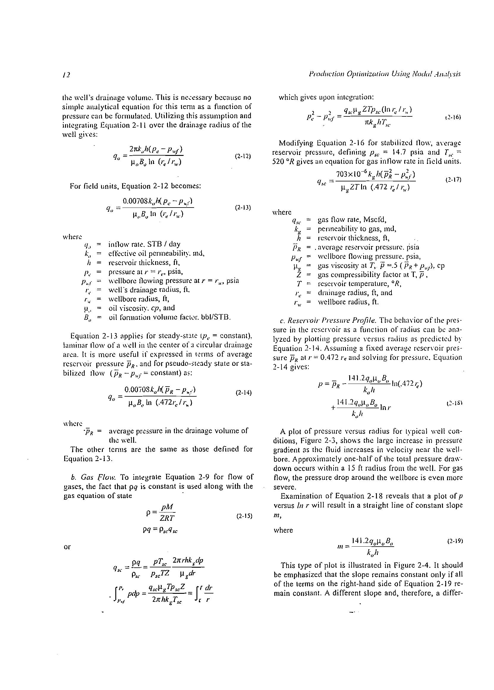
drainuge volumc. This is ne..:essary beca use no simple ílllalytical equation for this tenn as a functiol1 oC can be Utilizing this assumption and inlcgrating Equation 2-11 Qyer the drainagc radius of the wcll
2¡r.k.,h(p, - 1'''1)
llaBlJ 11'1 /1"11')
For fidd units, Equation 2-12 bccomes: (2-12)
(2-13)
where i/" k .. /¡ 1'.' p,,,. r "
i,,!lo\\' ml<, STB / day oil pcnneabiliIY. md, rcservoir lhickncss, n, prcssure al r = 1"1" psi a, wdlborc tlowing al r = r,.., psia wdl's drainage radius, fL \Vcllbore rJdíuS, n, oil \'iscosiry. cp, and oil fonll:Hiúl1 volulllc faclI..)f. bbl/STB.
Equatian 2-13 foe stcady-sr:.:.¡t (PI' = constant), laminar tlo\\' 01' a \\'dl in lhe ccnter of:.I circular drainngc arca. It is mOfe useful if exprcsscd in of rescr\'oir PRo and for s.tate or stabilized !lo\\' (PR - Puf:= constant) as:
- 1'",)
1l0B" / r,)
ProdllClioll 0plimizotioJl UsiJlg Noda/
which gives upon inlcgration:
Modifying Equalion 2-16 for stabilizcd no\\", reservoir presslLfc, defining Psc = 14.7 psia and T, •. =. 520 °R givcs un cquation for gas inf10w rate in ficld units. - 1',:,)
qsc = ' (2-17)
IlgLTln (.472 1;/1;,,)
where qsc k g h pR Puf Z T
gas tlow rate, Mscl'd, penncabililY lo gas, md, n::scn'oir thickness, n, averagc res,,:rvoir prcssurc. !)sia t10Willg psia, gas viscosiry al T, Ji =.5 (PR + PI')' cp gas compressibility factor at T, p , rescrvoir lcmperalurc, o R, drainuge radius, n, and wcllbore mdius, ft.
(2-14)
whcrc 'PR average in Ihe drJinage volume of well.
The other tcnns are the same as rhose defined for Equation 2-13.
b, Gas floa: To inh:grate Equation 2-9 for flow of gases, the faet that pq is constant is used along with the gas cquation of state
(2-15)
A plOl of prcssure versus radius for typical wcll conditiOllS, Figurc 2-3, shows thc large increasc in gradient <ls thl.: fluid illcrcases in vclocity ncar lhe we\lbore. Approximately one-half of lhe total pressllre dra\\'down occurs within a 15 ft radius from [he wcll. For gas t10w the pressllre drop around the wellborc is even more severe.
Examination of Equation 2-18 revea(s lhat a plOI of p versus In r will result in a straight hne of constant slope
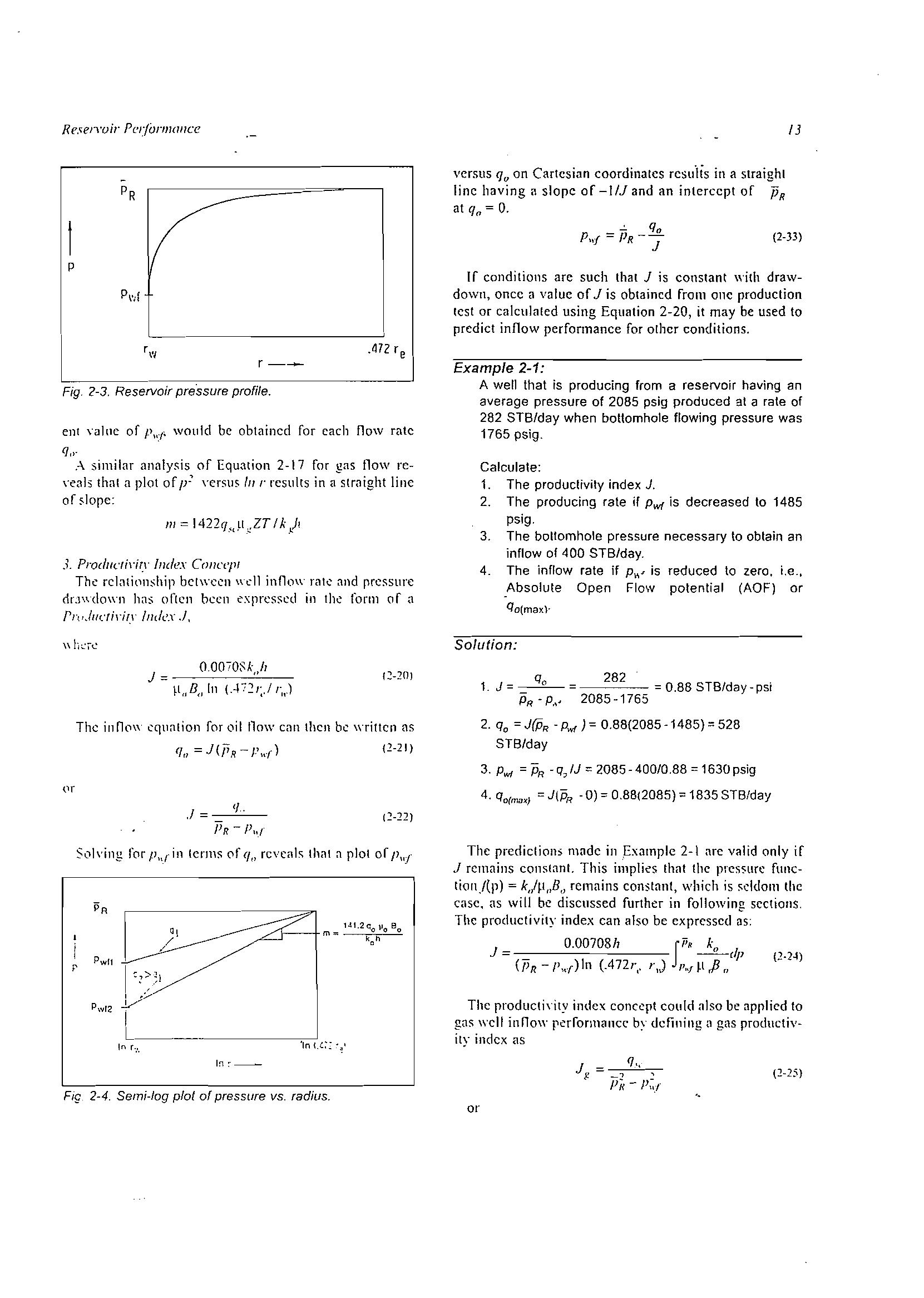
c. Resermir Pressure Profile. The behavior ol' presSlIfC in lhe rcscn'oir as a fUllction ol' radius can be ,:m3Iyzed by plouing pressurc verSus radius as predicleJ Equatiol1 }-14. Assuming a fixed average rescn·oir pressurc Px al r:= 0.472 and solving for pressure. Equarion 2-14 gives: m,
This type oC plol is illuSlratcd in Figure 2-4_ !I should be emphasizcd that the slope remains constant only if all oC the [erms on Ihe righl-hand side oC Equation 2-19 remain constan!. A different slope and, therefore, a differor
'"I!
p
I -::c r-
Fig. 2-3. Reservo;r pressure profile.
en! "aloe of P\l/' \Vould be obtaincd for each flo\V rate q".
A. similar anaiysis of Equation 2-17 for gas flo\V rc\'('als thnt a 1'101 of \'crsm'" r rcsu\ts in a strnight lille of :-.Iope:
3. Producrid(1' hule.\' Conccll/
The rclnlionship bctWCCll m:ll inflo\\' ralc and rrcssure dLl\\-clo\\'11 hns o((cI1 been t'xprcsscd in Ihe form of a r,.u)ucr;l·il.l· ¡lIdex./,
versus qf) on Cartcsian caardinatcs rcsu'¡is in a straighl line having" slopc of -IIJ and an ¡ntercepl of PR al qo = O.
(2·33)
Ir cond;tiolls are such tha[ J is constant ",illt drawdO\vl1, once a valuc of J is obtaincd from one production lest or calclIlated using Eqllation 2-20, it may be used to predict inflow performance ror other cOllditions.
Examp/e 2-1:
A wel1 that is producing from a reservoir having an average pressure of 2085 psig produced al arate of 282 STB/day when bottomhole flowing pressure was 1765 psig.
Calculate:
1. The productivily index J.
2. The producing rate ir Pwf is decreased lo 1485 psig.
3. The bollomhole pressure necessary lo oblain an inflow 01 400 STB/day.
4. The inflow rate if is reduced to zero, Le., Absolute Open FlolV polenlial (AOF) or qo(max)'
So/ution:
Thc inflc'l\\ equn(;on for oil !lo\\' cnll l!len be \\Tilten as qo =JCPR-P,,/) (2-21)
J = 00070:'k"h 111 r".) .1 = -=--,-<Je-' , 0, 282
PR - Pul
$0lving rOl' p,,(in tel'IllS ('Irq" rcv(,<lls Ilwl n plol or ¡J"f
Tlle predictiolls llliJdc in "Examplc 2-\ are val id only if J rcmains constan!. This implies tll<lt the prCS5urc function./{p) = k,/p"B" remains constant, which ;s scldol1l the case, as will be discussed further in following sections. Tlle productivity index can also be exprcssed as: J 0.0070817 sr, k" --dp (Pn -1"'l)ln (.472r,. r,) I"if ¡I j3"
(2·2-l) , ¡ r Pwfl
The producli\'ity index concept could <lIso be applicd to gas \\'ell inno,," by dcfining n gas productiv-ity indcx as
(2-25) or
703xlO-6 kgh
J g (2-26)
J.lgZTln
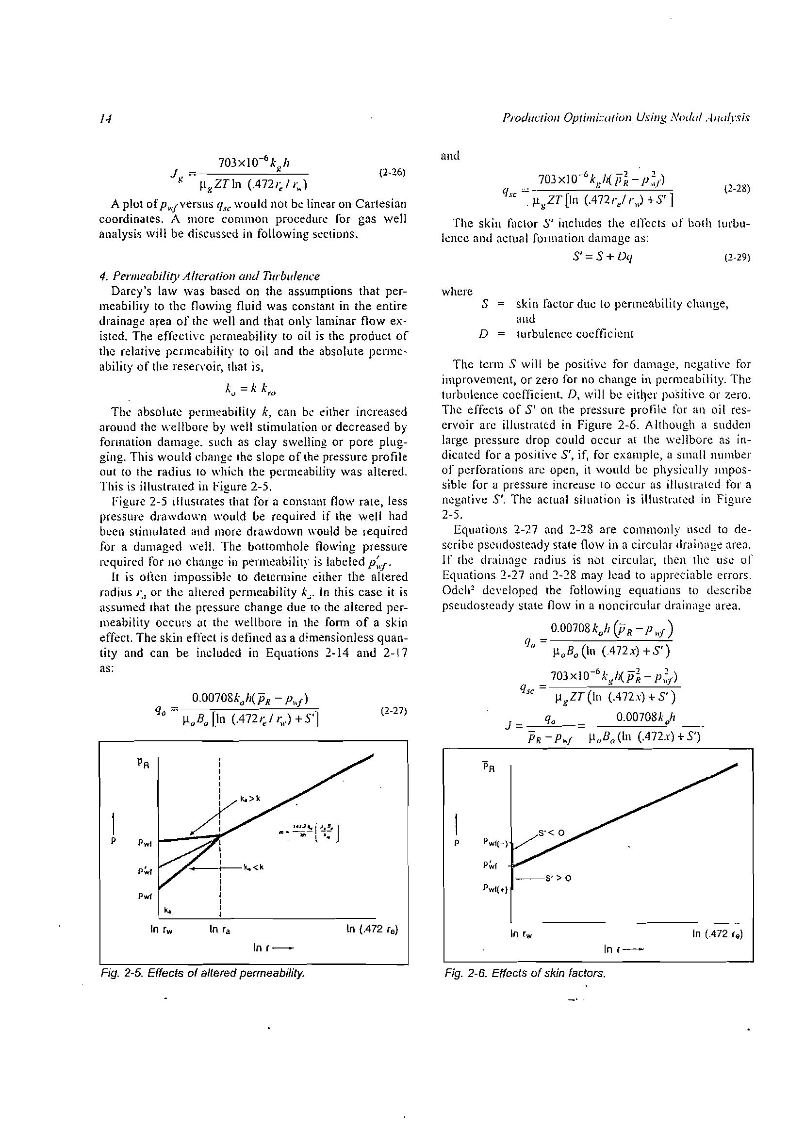
A plOI of liJe would not be linear 011 Cartesian coordinalcs. A more commoll procedure roc gas well anaiysis \ViII be discussed in following scctions. and
4. Permeability Altera/ion Clnd Turbulem:e
Darcy's law was bascd 011 the assumptions that permeability 10 (he nowing fluid was in lhe enlice drainage area ol' the well and that only laminar flow existcd. The effcctivc pcrmeability lo oil is lhe product of lhe fclativc permcability to oil and lhe absolute ability al' lhe reser\'oir, thal ¡s, k =k k ro
Thc absohuc pcrmeabilily k, can be either increased around [he wcllbofe by wcll stimulation oc decreased by fonnation damage. such as clay swelling oc pore plugging. This would changc Ihe slope of lhe pressure profile out to the radius lO which the pcrmeability was altered. This is illuSlrated in Figure 2-5.
Figure 2-5 illustrales that foe a CDIlSt.1nt flo\\' rate, less prcssure drawdown ",ould be cequired if the weJl had bccn slimulatcd and drawdowll would be requircd for a damaged wel!. The bottomhole tlowing pressure required for 110 changc in permcability is labelcd II is oftcn impossibk 10 delennine either the aItered mdius r. , 01" lhe alten.::d permeability k In this. case it is assumed Ihat the prcssure change due 10 the altered permeability oceurs al the wellbore in Ihe fonn of a skin cffee\. The skin effecl is defincd as a d!mensionless quantity and can be includcd in Equ3tions 2-14 and 2- t 7 as:
0.00708k)I(PR - p,,¡)
J.luSu [In (.4721; 11;,.) + S'] q,
2-5. Effects of allered permeability.
Prodm.:t;oJl Optinú::otiolJ Using Nodo! (2-28)
703xlO- 6 - P
q" = [In (.472rJ r,,) +S']
The ski n faclor S' inciudcs the crrccts uf both turbukncc ami actual fanuncion damagc as:
S' S + 0'1
whcre S ski n factor due lo pcrmcability change, <llld D turbulence cocfficicnt
(2-29)
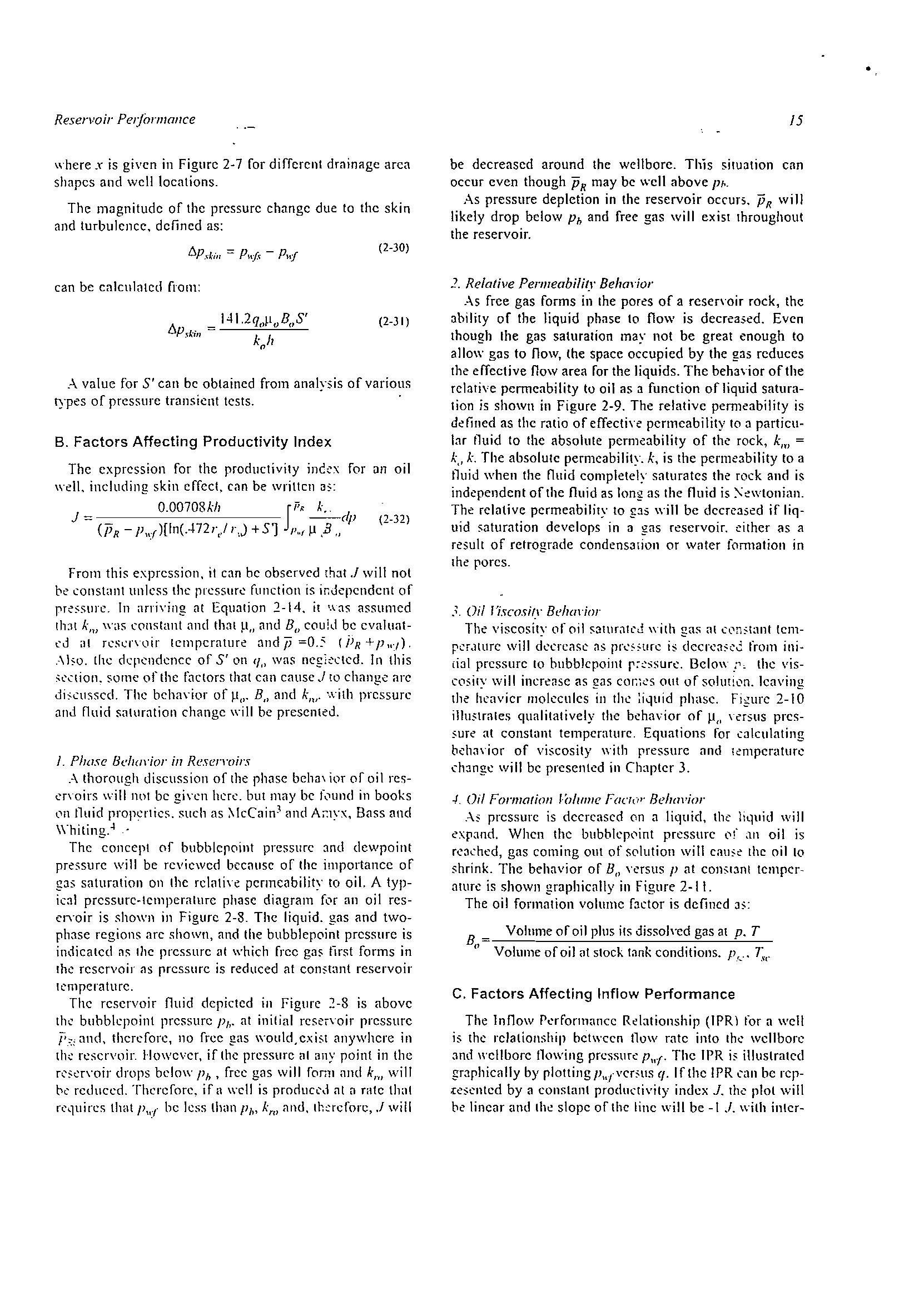
The tcrm S wil! be positivc ror damage, ncgati"c for improvemcnt, Dr zero for no changc in pcrmeability. The turbulcnce cocfficient. D, will be citller púsitivc 01' zera. Thc effccts oC S' on lhe pressure profik for an oil rescrvoir are illllstratcd in Figure 2-6. Althollgh a sudden large prcssurc drop cDuld occur al lhe wcllbore as indicated for a posilive 5', if, ror cxamplc, a small l1umber of pcrforations are open, it would be physically impossible for a pressure ¡necease lo occur as illustrated for a negative 5/, The actual siluarían is in Figure 2-5.
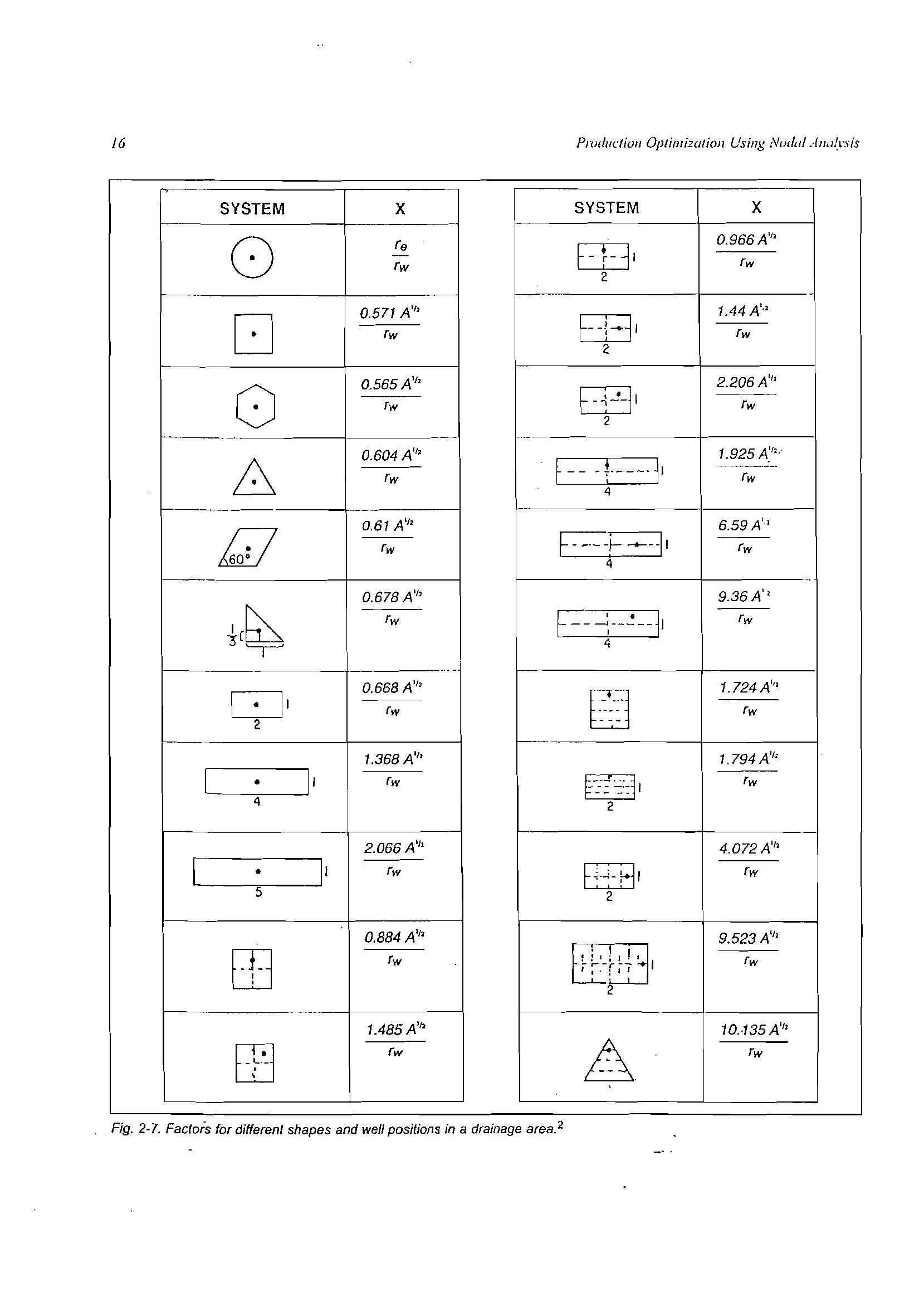
Equl.ltiDns 2-27 and 2-28 are cDl11l11only lIscd to describe psC'udostcady s{ate Oow in a circular drainagc area. Ir rhe drainage radíus is not circular, [hen Ihe use 01' Equations 2 27 and 2-28 rnay !cad to appreciablc errors. Odch 2 dc\'elopcd following equations to describe pseudostcady ::italc: t10w in a noneircular Jrainilgc (2-27)
0.00708 kjl (P R - P ,,¡ )
J.l,B, (In (472 x) +S')
J = -::-q-"",-p, - p,¡
J.luSo (In (.472x) + S')
2-6. Effacts of skin factors.
Fig.
Fig.
where x is givcn in Figurc 2-7 for diffcrcnt dr<'linagc arca shapcs and well locations.
The l11<lgnitudc of the pressure change due to the skin <'lnd turbulcncc. dcfined as:
can be ca1cul<llCd frol11:
be decreascd around the wellborc. This siluation can occur cven though PR may be wcll aboye 1"'.
As pressure deplction in the reservoir occurs. PR will likely drop bclow Ph and free gas \ViII exisr !hraughout the reservoir. (2-30)
l. ReJative Permeability Bellm"ior
:\ value for S' can be oblained from allalysis ofvarious types of prcssurc transíent tests.
B. Factors Affecting Productivity Index
The cxpress ion for the prodllctivity inc;?x for Lln oil wel!. including ski n cffcc!, can be writtcll 35: O.00708kh Si', k. I --(1' (PR - Puf )[ln(.-I72r/ r,) +Sl 1'", ,B"
From this exprcssion, il can be observcd willllot be constant uJlless lhe fUllction is ír:dcpcndcnt of rrc5surc. In arri\'ing ti! Eqllation 2-14. it 'Xas assul11ed Ih:Jt kili \Vas ('(lllstant ami that tlnd B/I c(lu1d be evalu<ltt·j íll rcscn-olr tcmpcrature andJj =0.:' (jJR+pU)). .-\}50. (he dcpcndcncc of S' on l/" wns negj;?cted. In lhis :'t'(lioll, sorne al' lhe that can cause J to chang.: are di:='cl1sscd. The bcha\·ior of 11ll' B" amI k,lJ 'xith prcssurc and nuid salur<ltion changc will be prescnted.
J. PITase Be}¡ul'ior in Reserl'Oirs
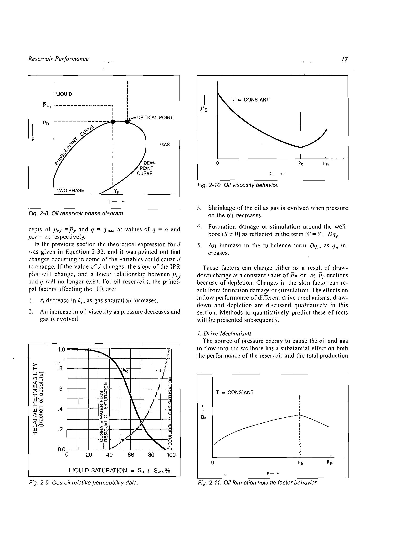
.-\ thorough discussion of lhe pllase beha\ ior of oil resc'fyoirs \ViII no! be giycn herc. bu! may be f 1tllHI in books \.111 tluid as and Ai":lYX. Bass and \\·hiting.-t _.
Thc conccpl of bubblcpClint prcssurc and dewpoitH pressure wil! be rcvie\Vcd bcctlusc of lhe importance of gas saturation on Ihe rchltiyt: pcrmc(lbility to oil. A typical pressurc·lcmperalure phase diagram f('lf nn oil res(,Iyoir is sho",n in Figure 2-8. Thc liquid. gas and tworhase regions arc 5hoWI1, <'lnd lhe bubblepoinl pressurc is indicated as the prcssurc al \\'hich free first forms in Ihe reservoir as rrcssurc is redllced at COll5tanl rescrvoir lemperaturc.
Thc rcscrvoir nuid dcpictcd in figure 2-8 is aboye lhe buhblcpaint pressurc p". at initial l"Csc,,·oir pressurc 1'_:;; élnd. thcrefore, no free gas \yould.exisl anywhcre in lh;: rcscrvoir. Ho\\'c"er, if lhe prcssurc nI an)' paint in lhe rcs.en·oir drops below I'h , free gas \ViII form ami km ",ril' relluced. Thcrcforc, if n \\'cll is produad al <l rate that rC\.luircs Ihat 1',,/ be Icss than I'h' km and, tL'rcforc,.J will
As free gas forms in lhe pores of a Tesen·oir rack, the abilily uf lhe ¡iquid phase lo no\\' is decreased. Evon though Ihe gas satura lío n may not be great enough to allow gas to Oow, (he space occupied by the gas rcduees the effective flow area for the liquids. The behavior ofthe rclative pcrrncability to oil as a function ofliquid saturalion is ShO\Vl1 in Figure 2-9. The relativc pemleability is delined as the ratio of effectiye pcnncability to a particu· lar fluid to the absolute pcrmeability of the rock, km = k" k. The absolutc permeability. k, is the permeability to a tluid when the nuid completely satura tes the roe k and is independent ofthe fluid as long as the fluid is :\ewtonian. The rclative pcrmeabiliry to g3.$ wil1 be dCCrC3$ed if liquid saturation develops in a gtls reservo ir. eilher as a result of retrograde condensalÍon or water ii.-¡mlatioll in ¡he pores.
., Oi¡ Bellador
The viscosity of oil w¡lh gas at tcmJ:'c-r.Hurc will d('clTase ;1$ is from ¡i::JI prcssurc lo bllbbkpoinl 8cI0\\-?, the vis("osilY \ViII increase as gas out uf SOlu!l011. lcaving lh? hcavicr molccllles in th(' :i(Juid pllasc. 2-10 iJlu5tmles qllalilalively the bchavior of 11" \-('[sus prcs5Ufe al constant tempcraturc. Equations for cJlculating bcha\·ior of vi$cosity with pressllrc <lnd lcmperature ch:mgc \ViII be presented in Chapter 3.
-l. Oi/ Forma/ion Vo/ume FacTo" Behm'ior
:\5 pressurc is decrcascd (ln a liquid. the liquid will expJnd. Whcn the bubblcpl1int pressure \.lf .111 oi! is reachcd, gas coming out ol' sC'lution \ViII the oil lo shrink. The behavior of 8 0 \'ersus ]J al C011:'13nl tcmpcrature js shoWIl grapllically in Figure 2-11.
The oil fonnalion voJume factor is dcfincd 35:
B Vollll11e of oil plus ils dissoh'cd gas al p. T 11 Volull1e of oil <Jt stock tan" conditiol1s.
e, Factors Affecting Infiow Performance
The lnno\V Pcrfonnnncc Rdationship (IPR) for a \\'ell is the rclalionship bet,,"ccn now rate into Ihe wcllbore and H'ellbore llowing prcssmc Pllf' The IPR is illuslrated graphically by plolting]J",.vcr511s q. (flhe IPR can be rep.resentcd by a constant productivily indcx J. pl01 \vill be linear and slope of the line will be -1 J. wilh inlcr-
2-7. Factors for differenl shapes and wel1 posiUons in a drainage 8(ea. 2
Fig.
uauro
Fig. 2-8. Oil reservoir phase diagram.
cepls of P"f =PR and q = (jm3x at valucs of q = o and p -¡ = o, respectively.
In the previous scction the Iheorctical express ion for J was gi\'en in Equation 2-32. and it W<lS pointed out that ..::hanges occurring in S0111e of the variables could cause J ¡l' change. Ir Ihe value of J changcs, the sh pc of the IPR plot will changc, and a linear rclntiol1shir betwecn Pul 3nd q "'jl! 110 longcr cxisl. For oil rcscr\"(lir:;. Ihe p31 f<lclC'fS <Irrccling the IPR are:
l.
A dccreasc in km as gas saturalion incre3scs.
An increase in oil viscosily as prcssure deereases and gas is evolved.
2-10. Oil viscosity behavior.
3. Shrinkagc of Ihe oil as gas is evolvccl when pressurc on the oil decrcases.
-.1. Formation damage or slimulalion around lhe wcllbore (5" O) as reflecled in lhe lerm S' 5 Dqo
5. An ¡ncrcase in Ihe lurbt11ence lcrm Dq{l4 as qo increases
Thcsc faetors can change either as a rcsult of drawdO\\"1l change at a constant \-alue of PR or as P.;: declines b-:l'ausc of dcpletion. Chang,;';, in the skin fJl'wr can rcsult from formation darnage t r stimulation. The em:cts on ¡nllo\\' performance ofdifferent drive mechanisms, drawd(,wl1 and dcplclion are discussed qualitilti\-ely in this section. Mcthods lo quantitativcly predict these ef-fecls wiJI be presentcd subsequently.
/. Dri\'e A1echoflisms
The sourcc of prcssure ent'rgy to c"use the ('jI and gas lo flow into lhe wcllbore has a substantial ctleer on both lhe performance of Ihe rcscryoir and the tolal production
Fig.
Fig. 2-9. Gas-oil relative permeabilily data.
Fig. 2-11. Oi/ formation vo/ume factor behavior.
-5yslcm. General dcscriptions of lhe basic types of drivc mc:chanisms are prescnted. Thc bchavior of rcservoir pressurc PR' lhe pressure function evaluated al p = ¡iR'/ (PR)' and surfacc producing gas/oíl ratio, R. Vt::fSUS cumulalivc n:covcry, N p , is presenlcd graphícaHy foc cach drive mcchanism.
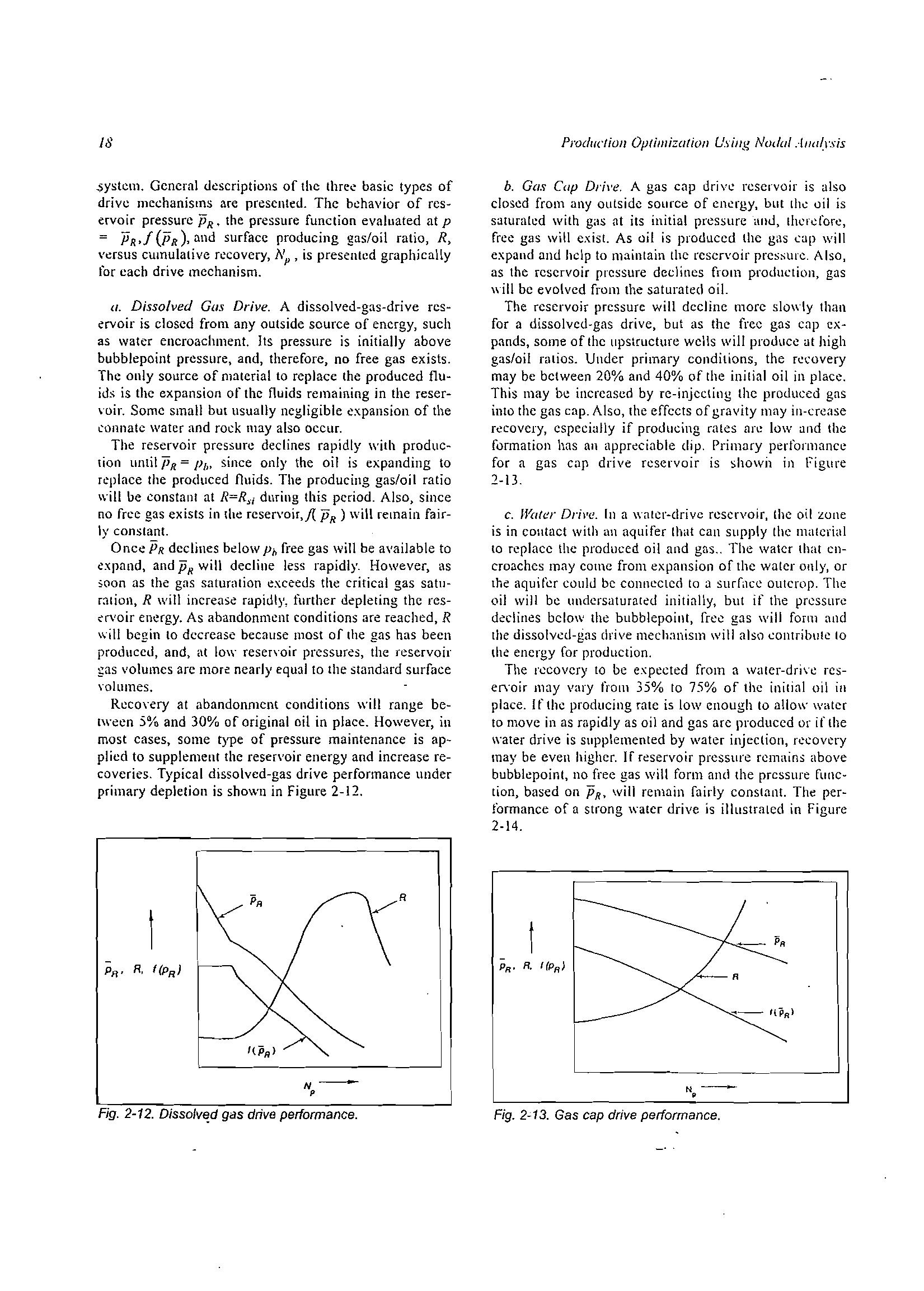
a. Dissolved Gas Drive. A dissolved-gas-drive rcservoir is closcd from any outside source of encrgy, such as water encroachment. Its pressure is initially aboye bubblepoint pressure, and, therefore. no free gas exists. The only source of material lo replace lhe produced fluids is lhe expansion ol' lhe fluids remaining in the reservoir. Sorne smal! bU{ usually ncgligible expansion of the connatc water and rock may also DCCUr.
The reservoir prcssurc declines rapidty with ¡ion ulllil PIl = PI» since onl)' the oil is expanding to the produced fluids. lile producing gas/oíl ratio wiII be constanl at during this periodo Also. sinee no free gas exisls in {he reser\'oir,j( PR ) will remain fair1)' constan!.
Once PR declines below Pb free gas wilI be available to expand, and PR will decline less rapidly. However. as SOOI1 as tlle gns satumlion exceeds tite critical gas satur:Hion, R will ¡nerease rapid!)', funher depleting the resrvoir energy. As abandomnent conditions are reached, R will begin lo dccrease because Illost of lhe gas has becn producco, and, at low resen·oir prcssures, the rcservoir gas volumes are more nearl)' egual to lhe standard surface yolumes.
Rcco\"cry at abandonmcnt conditions will range belween 5% and 30% of original oil in place. However, in most cases, some type of pressure maintenance is applicd to supplement the reservoir energy and ¡nerease recoycries. Typícal dissolvcd-gas drive performance under primary depletion is shO\\'n in Figure 2-12.
ProducliO/l Optimization Using Nodal
b. Gas CClp Driw. A gas cap rcscrvoir is also c10scd from any oulsidc SOllfce of cncrgy, but ¡ht: oil is sarura(¡;d wilh gas at its initial pressurc and, thcrt:rore, free gas wil! cxisl. As oil is produccd lile gas l:é1(l will expand and hc1p to maintain the rescr\'oir pressure. Also, as the rcscrvoir prcssure declines fmm production, gas will be evolvcd from the saturated oi!.
The rcscrvoir pressure will decline more slowly than ror a drive. but as the free gas cap expands, some of !hc llpstructure wclls wiIl produce <.It high gas/oil ralios. Under primary conditions, the rccovery may be bctwecn 20% and 40% of the initial oil in place. This may be increascd by rc-injecling the produced gas inlO the gas cap. Also, lhe effccts of gravity may in-crease rccovery, cspecially if producing rales un: low <.Ind the formarion has un appreciable clip. Primary performance for a gas cap drive reservoir is showi1 in Figure 1-13.
C. Water Dril'e. 111 a watcr-drivc rcscrvoir, lhe oil zone is in cOlltact with an aquifer that can supply the material te rcplace the prodllced oil and gas The water lhat CIlcroaches muy come from expansion of the water onl1', or the aquifcr could be connccled to a surface OUICWp. Thc oil wiJl be undcrsalurateu initinlly, but ir the prcssurc declines bclow the bubblepoint. free gas will form and the dissolvcd-gas ch·ive mechanism will also eontribu!e lo the encrgy ror produclion.
The rccovcry 10 be expected from a waler-dri\·e rcser\"oir may v.\ry from 35% to 75% of lhe initiZlI oil in pl:J.ce. 1f lhe producing rate is low cnough to allow water to movc in as rapidly as oil and gas are produced 01" if lhe water drive is sllpplemented by watcr injeclioll, rccovcry may be even higher. Ir reservo'r prcssurc rcmains aboye bubblcpoint, no free gas will form ane! the prcssure fUllCw !ion. based on PIl' \ViII remain fíJirly conslant. lhe perronnance of a strong water drive is illustralcd in Figure 2-14.