Essentials of business analytics 2nd edition camm solutions manual download

Predictive Data Mining

Essentials of Business Analytics

2nd Edition Camm Solutions Manual

Full download at link:

Test bank: https://testbankpack.com/p/test-bank-for-essentialsof-business-analytics-2nd-edition-by-camm-cochran-fryohlmann-anderson-isbn-1305627733-9781305627734/

Solution Manual: https://testbankpack.com/p/solution-manualfor-essentials-of-business-analytics-2nd-edition-by-cammcochran-fry-ohlmann-anderson-isbn-13056277339781305627734/

Chapter 9

Predictive Data Mining

Solutions:

a. The smallest classification error on the validation set results from the model: Log odds of using coupon = -8.049 + 0.001*Spending + 2.947*Card.

1.

b. The first decile lift of the model from part a is 5.135 (found by hovering cursor over first decile in decile-wise lift chart). For this test set of 200 observations and 37 coupon users, if we randomly selected 20 voters, on average (37/200)*20 = 3.7 of them would have used the promotional coupon. However, if we use the logistic regression model to identify the top 20 customers most likely to use the coupon, then we would identify (3.7)(5.135) = 19 of them that would use the coupon.

c. The area under the ROC curve is 0.9199. By hovering the cursor over the ROC curve, we see to achieve sensitivity of at least 0.80, 1 – Specificity = 0.0289 = Class 0 error rate.

a. Classification error is minimized at 9.5% for a value of k = 17.

2.

b. The area under the ROC curve is 0.9607. By hovering the cursor over the ROC curve, we see to achieve sensitivity of at least 0.80, 1 – Specificity = 0.0683 = Class 0 error rate.

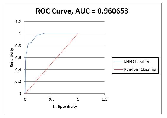
c. From the KNNC_NewScore worksheet, we see that the 17-nearest neighbors classifier predicts that 98 of the 200 customers in the Customer worksheet will use the promotional coupon.

a. The area under the ROC curve for the validation set is largest for the model: Log odds of dropping out = 0.3751 – 0.6332*GPA.

b. The students signing up for seminars on average have higher high school GPAs that the students who are not. Because high school GPA is positively related to staying in school (not dropping out), it is difficult to ascertain whether seminars are having any impact on drop-outs. That is, students already less likely to drop out are the ones enrolling in the seminars. To produce data that will allow Dana to better evaluate whether seminars indeed reduce the chance of students dropping out, administration should encourage at-risk students (low high school GPAs and other factors) to enroll in the seminars (perhaps giving these at-risk students first priority to enroll in the seminars).

a. For k = 1, the overall error rates on the training and validation sets are 0% and 6.87%, respectively. The overall error rate for the training set is computed by comparing the actual classification of each observation in the training set to the classification of the majority of the k most similar observations from the training set. Thus, for an observation (from the training set) and k = 1, the most similar observation in the training set is the observation itself. Therefore, if there are no observations with identical values of the input variables, k = 1 will lead to a 100% correct classification. However, if a training set has observations that have identical values of the input variables but different values of the output variable (Undecided), the training error will be nonzero (but typically small).

The overall error rate for the validation set is computed by comparing the true classification of each observation in the validation set to the classification of the majority of the k most similar observations from the training set. Thus, for k = 1, an observation (from the validation set) may not have the same classification as the most similar observation in the training, thereby leading to a misclassification.

b. The overall error rate is minimized at k = 5. The overall error rate is the lowest on the training data (3.28%) since a training set observation’s set of k nearest neighbors will always include itself, artificially lowering the error rate.

For k = 5, the overall error rate on the validation data is biased since this overall error rate is the lowest error rate over all values of k. Thus, applying k = 5 on the test data will typically result in a more representative overall error rate since we are not using the test data to find the best value of k For this particular data partition, we observe that the overall error rate on the test set is 5% which is slightly smaller than the overall error rate for the validation set (5.17%). Therefore, we can be confident that the overall error rate for the 5-nearest neighbor classifier is robust and conservatively about 5%.

c. The first decile lift is 2.50 (found by hovering cursor over first decile in decile-wise lift chart) For this test set of 2000 observations and 791 actual undecided voters, if we randomly selected 200 voters, on average 79.1 of them would be undecided. However, if we use k-NN with k = 5 to identify the top 200 voters most likely to be undecided, then (79.1)(2.50) = 198 of them would be undecided.

d. A cutoff value of 0.3 appears to provide a good tradeoff between the Class 1 and Class 0 error rates.

a. The full tree has 1.04% overall error rate on the training data because it continues branching until every terminal node consists wholly of a single class or until the minimum number of observations in a branch is less than 100. As this tree is very likely to be overfit to the training data, the best pruned tree is formed by iteratively removing branches from the full tree and applying the progressively smaller trees to the validation data. The best pruned tree is the smallest tree that achieves an overall error rate within a standard error of the tree with the minimum overall error rate.

5.

b. A 50-year old male who attends church, has 15 years of education, owns a home, is married, lives in a household of 4 people, and has an income of $150 thousand would be classified as Undecided (Class 1).

c. For the default cutoff value of 0.5 on the best pruned tree on the test data, the overall error rate is 2.05%, the class 1 error rate is 3.54%, and the class 0 error rate is 1.08%.

d. The first decile lift of the best pruned tree on the test data is 2.53 (found by hovering cursor over first decile in decile-wise lift chart) For this test data set of 2000 observations and 791 actual undecided voters, if we randomly selected 200 voters, on average 79.1 of them would be undecided. However, if we use best prune tree to identify the top 200 voters most likely to be undecided, then (79.1)(2.53) = 200 of them would be undecided.

a. Age is the most important variable in reducing classification error of the ensemble.

b. The overall classification error of the random trees ensemble is 8.4%, the Class 1 error rate is 19.60%, and the Class 0 error rate is 1.08%. Compared to the single (best pruned) tree constructed in Problem 5 (which had an overall error rate of 2.05%, a class 1 error rate of 3.54%, and a class 0 error rate is 1.08%), we observe that the random forests approach does worse

a. Using Mallow’s Cp statistic to guide the selection, we see that the models using 7 or 8 independent variables seem to be viable candidates. Using the validation set to compare the full model (with all 8 variables) to the model with 7 variables (dropping Married), we observe that the results are very similar. The full 8-variable model correctly identifies three more Class 1 observations, but correctly identifies eight fewer Class 0 observations. Comparing the decile-wise lift charts, both models achieve a lift of 2.47 on the first decile. On the second decile, the 7-variable model achieves a lift of 2.29 while the 8-variable model achieves a lift of 2.28. Because both models have similar effectiveness, we select the simpler 7-variable model.

Full (8-variable, 9-coefficient) model: 7-variable, 8-coefficient model:

The resulting model is: log odds of being undecided = -3.849 – 0.012*Age + 0.580*HomeOwner + 1.199*Female + 0.220*HouseholdSize – 0.006*Income + 0.205*Education – 1.666*Church.

b. Voters with more household members, more education, and who are homeowners and female are more likely to be undecided. Older voters with higher incomes and who attend church are less likely to be undecided.

c. The overall error rate of the 7-variable model on the test set is 25.15%.

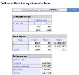
a. Churn observations only make up 14.49% of the data set. By oversampling the churn observations in the training set, a data mining algorithm can better learn how to classify them.

b. A value of k = 19 minimizes the overall error rate on the validation set.

c. The overall error rate on the test set for k = 19 is 12.11%.

d. The class 1 error rate is 20.62% and the class 0 error rate is 10.66% for k = 19 on the test set

e. Sensitivity = 1 – class 1 error rate = 79.38%. This means that the model can correctly identify 79.38% of the churners in the test set. Specificity = 1 – class 0 error rate = 89.34%. This means that the model can correctly identify 89.34% of the non-churners in the test set

9.

f. There were 61 false positives (non-churners classified as churners). There were 20 false negatives (churners classified as non-churners). Of the observations predicted to be churners, 61 / (61 + 77) = 44.20% were false positives. Of the observations predicted to be non-churners, 20 / (20 + 511) = 3.77% were false negatives.

g. The first decile lift is 4.08. For this set of 669 customers, there are 97 actual churners. Thus, if we randomly selected 67 customers, on average 9.7 of them would be churners. However, if we use kNN with k=19 to identify the top 67 customers most likely to be churners, then (9.7)(4.08) = 40 of them would be churners.

a. Churn observations only make up 14.49% of the data set. By oversampling the churn observations in the training set, a data mining algorithm can better learn how to classify them.

b. The full tree (with 41 decision nodes) has 6.85% overall error rate on the training data. Note that the error rate is not 0% because the full tree is restricted to 7 levels (before each leaf node consists entirely of a single class). As this tree is very likely to be overfit to the training data, the best pruned tree is formed by iteratively removing branches from the full tree and applying the progressively smaller tree to the validation data. The best pruned tree is the smallest tree that achieves an overall error rate within a standard error of the tree with the minimum overall error rate.

c. Churners are categorized by:

i. Customers with more than 3.5 customer service calls and fewer than 187.4 daytime minutes OR

ii. Customers with more than 3.5 customer service calls, greater than 187.4 daytime minutes and monthly charges > $62.50 OR

iii. Customers with more than 3.5 customer service calls, greater than 225.1 daytime minutes and monthly charges < $62.50 OR

iv. Customers with fewer than 3.5 customer service calls, between 220.1 and 227.9 daytime minutes, monthly charges > $59.15, data usage > 1.92 GB, and have held an account for less than 135 weeks OR

v. Customers with fewer than 3.5 customer service calls, greater than 220.1 daytime minutes, monthly charges > $59.15, data usage < 1.92 GB, and an overage fee over $7.825 in the last 12 months OR

vi. Customers with fewer than 3.5 customer service calls, greater than 220.1 daytime minutes, monthly charges < $59.15, and an expired contract OR

vii. Customers with fewer than 3.5 customer service calls, less than 220.1 daytime minutes, an expired contract, and roaming minutes > 13.05 OR

viii. Customers with fewer than 3.5 customer service calls, between 76.2 and 220.1 daytime minutes, an expired contract, and roaming minutes < 13.05, and data usage < 3.265 GB

d. The overall error rate is 15.84%. The class 1 error rate is 15.46% and the class 0 error rate is 15.91%.

e. The first decile lift is 3.87 (found by hovering cursor over first decile in decile-wise lift chart) For this set of 669 customers, there are 97 actual churners. If we randomly selected 67 customers, on average 9.7 of them would be churners. However, if we the classification tree to identify the top 67 customers most likely to be churners, then (9.7)(3.87) = 38 of them would be churners.

a. The most important variable in reducing classification error of the ensemble is the number of weeks the customer’s account has been active.

b. The overall classification error of the random trees ensemble is 15.10%, the Class 1 error rate is 12.37%, and the Class 0 error rate is 15.56%. Each of these error rates are smaller than the corresponding error rates for the single (best pruned) tree constructed in Problem 9 (which had an overall error rate of 15.84%, a class 1 error rate of 15.46%, and a class 0 error rate is 15.91%.

a. Churn observations only make up 14.49% of the data set. By oversampling the churn observations in the training set, a data mining algorithm can better learn how to classify them.

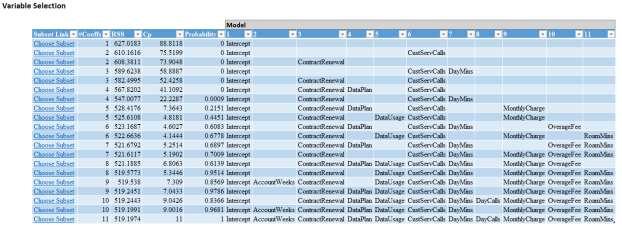
b. Using Mallow’s Cp statistic to guide the selection, we see that there are several viable models for consideration. We will compare two different models based on the validation set: (i) a fivevariable model with ContractRenewal, DataUsage, CustServCalls, MonthlyCharge, and RoamMins, and (ii) a four-variable model with ContractRenewal, DataUsage, CustServCalls, and MonthlyCharge.

We observe that 5-variable model correctly classifies two more Class 1 observations than the 4variable model, but correctly classifies six fewer Class 0 observations. The first- and second-decile lifts for the 5-variable model are 3.03 and 2.48, respectively. The first- and second-decile lifts for the 4-variable model are 2.90 and 2.55. These models are comparable, but we choose to proceed with the 5-variable model due to its first-decile lift advantage.

5-variable, 6-coefficient model: 4-variable, 5-coefficient model:

The resulting model is: log odds of churning = -2.95 – 2.61*ContractRenewal – 1.05*DataUsage + 0.62*CustServCalls + 0.07*MonthlyCharge + 0.07*RoamMins.

If a customer has recently renewed her/his contract, the customeris less likely to churn. If a customer uses a lot of data on her/his plan, the customer is less likely to churn. If a customer makes many customer service calls, the customer is more likely to churn (these calls suggest the customer is unhappy with the cell service). If a customer’s monthly charge is high, the customer is more likely to churn. An increase in roaming minutes also increases the likelihood of churning.

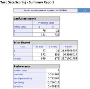
c. The overall error rate is 25.71% on the test set.

a. The value of k = 17 minimizes the RMSE on the validation data.

b. The RMSE = 55.95 on the validation set and RMSE = 51.52 on the test set. This is an encouraging sign that the RMSE of k = 17 on new data should relatively stable and in the range of 51 to 56

c. The average error on the test set is 0.04 suggesting there is essentially no bias in the prediction. That is the predicted credit scores over- and under-estimate equally likely. A histogram of the residuals shows that the prediction error is roughly symmetric around zero (slightly skewed to the left).

a. The best pruned tree achieves an RMSE of 57.87 on the validation set and 55.99 on the test set It is encouraging that the RMSE on the validation set and test set are very similar. This suggests that RMSE on new data will be approximately 55 to 58.

b. The best pruned tree predicts a credit score of 698 for the individual who has had 5 credit bureau inquiries, has used 10% of her available credit, has $14,500 of total available credit, has no collection reports or missed payments, is a homeowner, has an average credit age of 6.5 years, and has worked continuously for the past 5 years.

c. Decreasing the minimum number of records in a terminal node to 1 results in a 14-node best pruned tree with a RMSE of 55.75 on the test data. This is just a 0.4% reduction in RMSE of 55.99 resulting from the 11-node best pruned tree from part a (using 244 as the minimum number of records in a terminal node). Therefore, we see that increasing the levels in a regression tree and allowing the terminal nodes to be based on fewer observations can decrease the prediction error, but there is a decreasing marginal benefit to decreasing the granularity of the tree.

14. The root mean squared error of the random forest of regression trees is 55.71 which is slightly smaller than the root mean squared error of 55.75 for the single best pruned tree in part a of Problem 13

a. Using Mallow’s Cp statistic to guide the selection, we see that one of the models using 2 independent variables is a strong candidate. Based on classification error on the validation set, we also observe the model with 2 independent variables (OscarNominations and GoldenGlobeWins) has the same classification error as the model with 3 independent variables OscarNominations, GoldenGlobeWins, and Comedy)

The resulting model is: log odds of winning = -8.21 + 0.57*OscarNominations + 1.03*GoldenGlobeWins.

If a movie has more total Oscar nominations across all categories, it is more likely to win the Best Picture Oscar. If a movie has won more Golden Globe awards, it is more likely to win the Best Picture Oscar

b. The sensitivity of the logistic regression model is 22.22%. Of the nine Oscar winners in the validation set, the model correctly identifies 2 of them. This is a good measure to evaluate a model for this problem as we are most interested in identifying the annual winner.

c. By using a cutoff value to classify a movie as a winner or not, in some years the model may not classify any Best Picture Oscar winner or may classify multiple Best Picture Oscar winners. For example, below we see that the model does not predict any movie to win in 2006.

d. For each year, identify the movie with the highest probability of being the winner and make that the model’s sole “pick” for winner. Doing this results in identifying three correct winners in the nine years of validation data. That is, the sensitivity of the model is (3/9) = 33.33%. The analyst should perhaps consider additional variables to classify Best Picture Oscar winners.

e. The model predicts that “Birdman” is the movie most likely to win the 2014 Best Picture Award. As listed in the NewDataToPredict worksheet, “Birdman” indeed won the 2014 Best Picture Award, so this is a correct classification if we use the “maximum probability” approach to identify the winner.

i. A value of k = 7 minimizes the RMSE on the pre-crisis validation data.

16.

a.

b.

iii. The average error on the validation set is $3,119 and the average error on the test data is $3,988. This suggests that the k-NN model tends to under-estimate the price of a home. This is likely due to the fact that there are very few expensive homes in the pre-crisis data set so the predicted prices of these homes are vastly under-estimated.

i. A value of k = 4 minimizes the RMSE on the post-crisis validation data.

ii. The RMSE on the validation set is $23,389 and the RMSE on the test data is $27,268

iii. The average error on the validate set is $1,290 and the average error on the test data is $2,831. This suggests that the k-NN model tends to under-estimate the price of a home. This is likely due to the fact that there are very few expensive homes in the post-crisis data set so the predicted prices of these homes are vastly under-estimated.

c. The average percentage change = -2.42%. Predicted sales price based on post-crisis data is on average 2.42% lower than predicted sales price based on pre-crisis data.

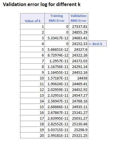
ii. The RMSE on the validation set is $24,152 and the RMSE on the test set is $24,396.

i. There are 107 decision nodes in the full tree and 29 decision nodes in the best pruned tree.

ii. The RMSE on the validation set is $20,402 and the RMSE on the test data is $23,169.

iii. The average error on the validation set is $385 and the average error on the test data is $295 There is very slight evidence of systematic under-estimation of home price, but by only 1% - 2%.

iv. The best pruned tree for the pre-crisis data contains decision nodes on BuildingValue, Age, PoorCondition, LandValue, AboveSpace, Acres, and Deck

b.

i. There are 104 decision nodes in the full tree and 16 decision nodes in the best pruned tree.

ii. The RMSE on the validation set is $22,307 and the RMSE on the test data is $22,216

iii. The average error on the validation set is -$1017 and the average error on the test data is -$456 The regression tree seems to slightly over-estimate price of post-crisis homes.

iv. The best pruned tree for the post-crisis data contains decision nodes on BuildingValue, LandValue, AC, and AboveSpace.

c. The average percentage change = -3.55%. Predicted sales price based on post-crisis data is on average 3.55% lower than predicted sales price based on pre-crisis data.

a. Using goodness-of-fit measures such as Mallow’s Cp statistic and adjusted R2, we see that there are several viable models for consideration. After comparing several of the candidate models based on prediction error on the validation set, we suggest that includes 8 independent variables is a strong candidate.

i.

ii. The RMSE on the validation set is $16,863 and the RMSE on the test data is $16,709

iii. The average error on the validation set is $622 and the average error on the test data is $173. There is very slight evidence of systematic under-estimation of home price.

b. Using goodness-of-fit measures such as Mallow’s Cp statistic and adjusted R2, we see that there are several viable models for consideration. After comparing several of the candidate models based on prediction error on the validation set, we suggest that includes 9 independent variables is a strong candidate.

i.

ii. The RMSE on the validation set is $18,403 and the RMSE on the test data is $17,321.

iii. The average error on the validation set is -$692 and the average error on the test data is -$70. Estimates of home price using the post-crisis data appear to have a very slight bias towards over-estimation.

c. The average percentage change = -5.43%. Predicted sales price based on post-crisis data is on average 5.43% lower than predicted sales price based on pre-crisis data.