
Engineering Electromagnetics and Waves 2nd edition by Inan Said ISBN 0132662744
9780132662741
Download solution manual at:
https://testbankpack.com/p/solution-manual-for-engineeringelectromagnetics-and-waves-2nd-edition-by-inan-said-isbn-01326627449780132662741/
6
The Static Magnetic Field
6.1 Force between two infinitely long wires.
Following a similar approach as in Example 6.1, the magnetic repulsion force per unit length experienced by each wire can be written as
from which we
6.2 Forces betweentwo wires.
Two wires of a transmission line carry oppositely directed current and therefore experience magnetic repulsion, which can balance electrical attraction, due to opposite charges induced on the wires. The electric field produced by wire 1 at the location of wire 2 is given by (see Example 4.12 and Figure 6.1 below)
The electrostatic force exerted on a unit length portion of wire 2 is thus given by
We can express this force in terms of the applied potential difference V0 by using the per unit length capacitance of this configuration. From Example 4.29 we have
Chapter 6/ The Static Magnetic Field
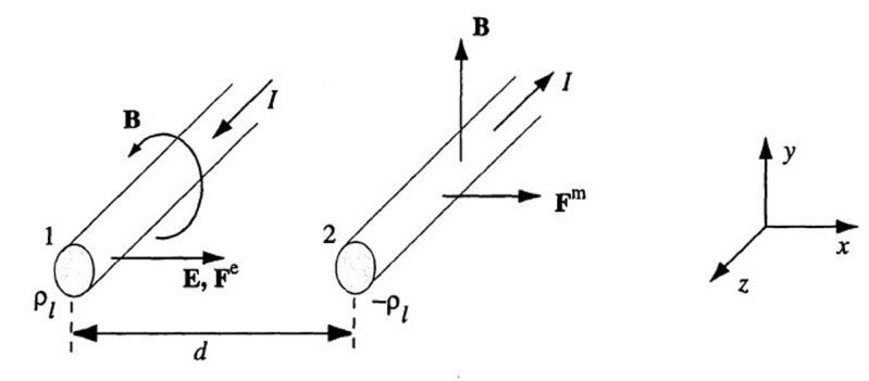
since the separation of the wires (d = 1 cm) is much larger than the wire diameter (2a = 1 mm). The magnetic force exerted by wire 1 on a unit length portion of wire 2 is (see Example 6.1)
For balance between the two forces we must have
Substituting the values yields I ≃ 27 9 mA.
6.3 Bundle clash in a transmissionline.
Assuming the wires to be infinitely thin (since 50 cm ≫4 cm) andfollowing a similar approach as in Example 6.1, the peak magnetic force of attraction per unit length on each wire can be calculated
To get a better feel about the strength of this peak force, consider this force as being the weight of an object which has a corresponding mass given by m = F/g ≃ 4000/(9 81) ≃ 408 kg. Assuming a typical person weighs about 70 to 80 kg, the peak attraction force is equivalent to the total weight of about 5 to 6 persons. That is, the peak force of attraction exerted over 1 m length of each wire can be thought of as the force that would be exerted on the wire if 5 to 6 people were to stand up over 1 m portion of this wire. Therefore, this strong peak attraction force may well make the wires in the bundle to collapse onto one another and cause the bundle to clash.
6.4 Magnetic force between current elements.
The differential force between two current elements is given by the integrand in equation (6.1), namely
where dF12 is the force exerted by element 1 on element 2 and R
is the unit vector from element 1 to element 2.
(a) Taking the origin to be at the location of element 1, we have
(b) For this case the problem statement and the figure in the text fail to specify the distance between the two elements. For the purposes of our solution here, we shall take this distance to be a We then have
6.5 Square loop.
Consider a square loop carrying a current I. To find the total magnetic force on each side, we use (6.1) where Idl2 × (Idl1 × R) is a vector which is always perpendicular to and outward from each side of the square loop. So, the total force on each side calculated from (6.1) is perpendicular to that side and outward from it and as a result, the loop has a tendency to expand.
6.6 Force on a current-carryingwire.
Assuming the earth's magnetic field of B0 ≃ 0 5 G to be in the y direction and the current I = 1 kA to be flowing in the x direction, the force per meter on the current-carrying conductor exerted by the earth's B field can be found as
6.7 Rigid rectangularloop.
(a) We assume the current in the rectangular loop to be flowing in the clockwise direction, as shown in Figure 6.2. For I = 5 A and B = ˆ xB0 =
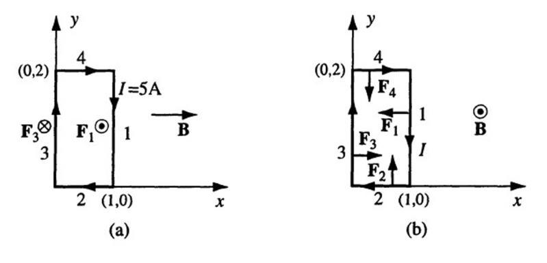
x1 5 T, the forces on sides 1, 2, 3, and 4 can be calculated using a similar approach as in Example 6.2 as
(b) Following a similar approach as in part (a) with B = ˆ z1 5 T, the forces on sides 1, 2, 3, and 4 can be found as F1 = F3 = ˆ x15 N and F2 = F4 = ˆ y7 5 N respectively.
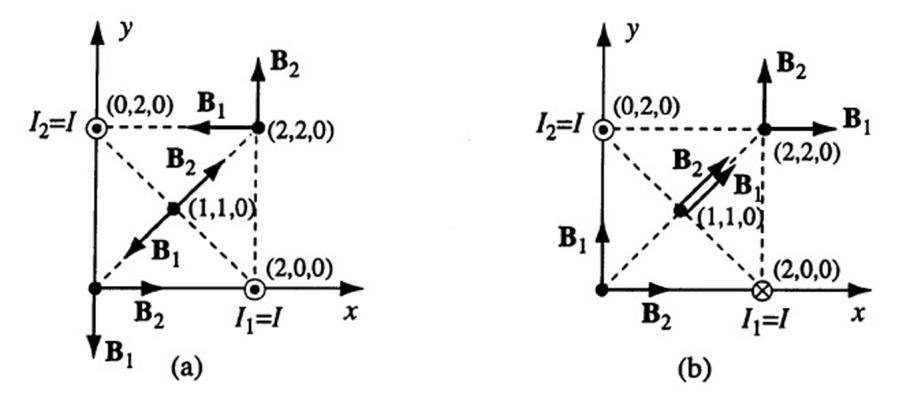
6.8 Two parallel wires.
(a) Using the superposition principle, the B field at the origin is given by
(b) The B field at point (1,1,0) can be written as
(c) Similarly, the B field at point (2,2,0) can be found as
(d) When the direction of the current on the x axis is switched, all the B1 fields also switch direction. Thus, the B field at the origin is now given by
point (2,2,0) follows as
6.9 An infinitely long L-shaped wire.
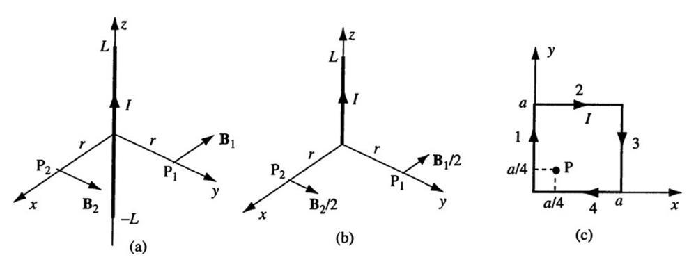
(a) We can consider the L-shaped wire as two wires, one from the origin to x = ∞ and the other from the origin to y = ∞ and apply the superposition principle. Assume the current flowing from x = ∞ to y = ∞. At point P1( a, 0, 0), no B field is produced due to the x portion of the L-shaped wire since the observation point P2 lies along the x axis. The B field produced by the y portion of the L-shaped wire at P1 can be found from Example 6.3 by changing z to y, z ′ to y ′ , r direction to x direction, z ′ = a to y ′ = 0, and z ′ = a to y ′ = ∞, yielding
(b) Following a similar approach for point P2(0, a, 0), since P2 lies on the y axis, only the x portion of the L-shaped wire produced B at point P2 given by
Chapter 6/ The Static Magnetic Field
(c) At point P3(0, 0, a), both the x and y portions of the L-shaped wire contribute to the B field resulting in
6.10 B-field in a cylindrical conductor.
(a) Using the differential form of Amp` ere's law given by (6.11) as
we can easily compute J by noting that B only contains a
component that varies with r, so
The total current I passing through the conductor is given by (5.1) as
(b) Applying Amp` ere's law given by (6.9):
and noting the cylindrical symmetry, we can evaluate the azimuthal component of B as
6.11 Irregularloop.
We consider each side of the loop by itself and apply the superposition principle. Since point P lies on the axes of two of the sides of the loop, the current flowing in those sides do not contribute any B field at point P. Using the result of Example 6.7 and assuming the z direction to be out of the page, the B field produced at point P by current flowing in the closest side of the loop is given by
Similarly, the B field contributed by the current
owing in the farthest side is
Therefore, the total B field at point P due to the current in the loop follows as
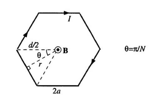
6.12 An N-sided regular loop.
(a) We consider each side of the N-sided polygon-shaped loop separately and apply the superposition principle. Note that due to symmetry, the magnetic field due to the current of each side is the same. Using the result of Example 6.3 with Figure 6.4, the magnitude of the total B field produced at the center of the loop can be written as
where we replaced
(b) As N → ∞, tan(
/N) ≃
/N and as a result, we find
which is the same result obtained in Example 6.6.
6.13 Square loop of current.
In this and some of the other problems in this chapter, it is useful to note that, as depicted in Figure 6.5a and 6.5b, the B-field at some distance r from the edge of a current carrying wire of length L is one-half of that at the same distance r from the center of a wire of length 2L, the expression for which was derived in Example 6.3. Namely,
field at a distance r from the center of wire of length 2L
Chapter 6/ The Static Magnetic Field
On this basis, the contributions of each side of the square depicted in Figure 6.5c can simply be formulated as the superposition of the B-fields at various distances from edges of wires of lengths L = a/4 and L = 3a/4. We first note that the contributions due to segments 1 and 4 are equal, as are those from 2 and 3. Using the right-hand rule, it is clear than all segments produce a B-field at point P in the z direction, so that the different contributions can be simply added to find the total field. We have
6.14 A wire with two circular arcs.
We consider each portion of the loop separately and apply the superposition principle. The straight portions do not produce any B field at point P since P lies along their axis. Assuming the z direction to be out of the page, the B field at point P produced by the current in the circular-arc portion with radius a is
Similarly, the B field produced by the current in the circular arc with radius b is
Therefore, the total B produced by the wire loop is
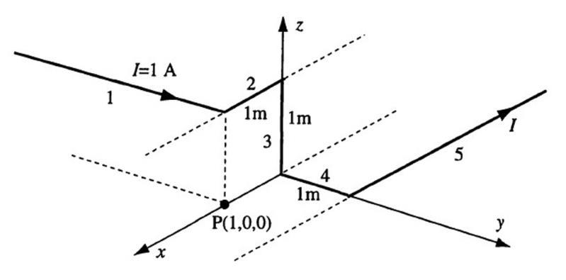
6.15 Wire with four 90◦ bends.
With reference to Figure 6.6, and the result of Example 6.3 the B-field at point P can be determined as a superposition of the contributions from different segments 1 through 5. The two formulas used are:
Designating Bi as the contribution to the B-field at point P by the ith wire segment we have
Chapter 6/ The Static Magnetic Field
6.16 Infinitelylong copper cylindrical wire carrying uniform current. Using the results of Example 6.10 with I
we have
10 Chapter
6.17 Helmholtz coils.
From Example 6.6, we know that the B-field at a point along the axis of a circular current carrying loop of radius a is
where z is the distance from the loop center, and the z-axis has chosen to be in the direction of the thumb, when the right-hand fingers move in the direction of the current flow in the loop.
(a) Consider a point P(0,0,z) along the z axis at a distance of z from the center of the loop on the left in Figure 6.59 on page 524 of the text. The distance between this point P and the center of the loop on the right is then (d z). The B-field at this point P is then given as the superposition of the contributions from the two loops, namely
where we have taken note of the fact that both of the loops have N turns.
Chapter 6/ The Static Magnetic Field
Following the same procedure as given above, and with some patience, it is a rather straightforward and useful exercise for the student to differentiate the d2Bz/dz2 expression given above and show that d3Bz/dz3 = 0 for z = a/2.
The natural question to ask at this point is whether the fourth derivative is also zero. It can be shown by expanding the expression Bz(z) around z = a/2 that given by
so that d4Bz/dz4 = 0. The fact that the first three derivatives are zero provides for an extremely smooth and uniform magnetic field, which is the basic motivation for using the Helmholtz coil configuration.
(d) We have
For d = a, the field at the midpoint (z = a/2) is
(e) At the center of the coil on the left (z = 0) we have
which is quite close to the approximate expression given for the mid-point, underscoring the purpose of the Helmholtz coil configuration, namely to establish a B-field which is very nearly uniform.
Note that by symmetry, the B-field at the center of the coil on the right (z = a) must be the same.
6.18 Helmholtz coils.
Using the midway-point Bz expression provided in Problem 6.17 with Bz = 100 µT, I = 1 A, and
6.20
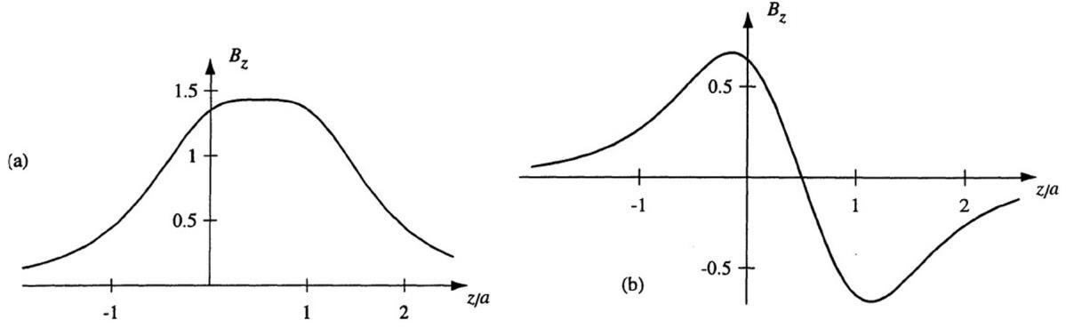
Using the result of Example 6.6, we simply switch the sign of one of the magnetic fields to find:
which is plotted as a function of z/a in Figure 6.7b. For comparison, Figure 6.7a shows bz(z) versus z for the case when the currents in the coils flow in the direction shown in Figure 6.59. We see that Bz is quite uniform for the latter case but that this uniformity is completely destroyed when one of the currents is reserved.
The configuration of the square Helmholtz coils is shown in Figure 6.8a. To determine the B-field at any point P along the axis, we rely on the result found in Example 6.3 for the B field at a distance r from the center of a current carrying wire of length a, namely
For the case in hand, we have r = R, and by symmetry, it is clear that only the projection of the field along the z axis (i.e., its z component) is nonzero. Thus, the z component of the B field produced by one of the lower square coil is
region near the maximum for d = 0 5a, 0 5445a, and 0 6a.
The total due to the lower loop is 4B1z and that due to the upper loop is identical except for the fact that the center of the loop is at distance (from P) of (d z), rather than z. Thus, the total B field at point P due to both of the square loops (both assumed to be carrying currents I, flowing in the same direction so that they produce fields in the same direction at point P) is then
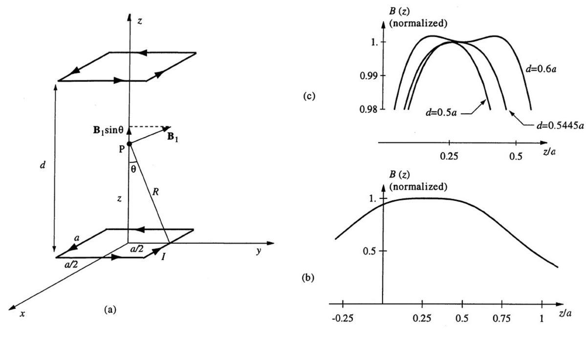
where we have taken into account the fact that both of the loops have N turns. Figure 6.8b shows a plot of the normalized B field (i.e., B(z)/Bmax) as a function of z for d = 0 5445a. To demonstrate that this is indeed the optimum spacing for which the field variation is the smoothest (i.e., d2B(z)/dz2 = 0), an expanded view of the region near the maximum is shown in Figure 6.8c for d = 0 5a, 0 544a, and 0 6a We see clearly that d = 0 5445a case is smoother than d = 0 5a and the distribution is already double-peaked for d = 0 6a, indicating that this separation is larger than optimum.
In comparing the results of this problem with those of Problem 6.17, it is useful to note that the optimum spacing of d = a for circular coils of radius a is only slightly different from the optimum spacing of d = 0 5445a for square coils of side-length a Physically, square coils of side length a should be compared with circular coils of radius a/2, for which the optimum separation is d = 0 5a
6.21 A circular and a square coil.
Figure
and calculation of the Bfield. (b) Normalized Bz(z) versus z for the case in hand, i.e., a square and a circular coil. (c) Normalized Bz(z) versus z for two circular coils.
The configuration of the square Helmholtz coils is shown in Figure 6.9a. To determine the B-field at any point P along the axis, we reply on the result found in Example 6.3 for the B field at a distance r from the center of a current carrying wire of length L, namely
For the case in hand, we have r = R, and L = 2a, and by symmetry, it is clear that only the projection of the field along the z axis (i.e., its z component) is nonzero. Thus, the z component of the B field produced by one side of the square coil is

Chapter 6/ The Static Magnetic Field
The total field on the square loop is Bsqr = 4B1z. To determine the contribution due the circular coil, we rely on the result of Example 6.6, specifying that the B-field at a point along the axis of a circular current carrying loop of radius a is
where z is the distance from the loop center. Since the distance between point P in Figure 6.9a and the center of the circular loop is (d z), the B-field at point P due to the circular coil is
The total B-field at point P due to both the square and circular coils is then
The normalized amplitude of the B-field is plotted versus z in Figure 6.9b for d = a. For comparison, a similar plot for two circular coils of radius a are shown in Figure 6.9c. We note that the field for the two circular coils is somewhat smoother near the origin (i.e., near z = 0 where the square coil is located).
6.22 Magnetic field of a solenoid.
This is a very long solenoid since l = 40 cm ≫2 cm = a.
(a) Using the results of Section 6.2.1 on page 436 of the text, with N = 350 and I = 1 A, the B field at the center of the solenoid can be approximately calculated as
(b) Similarly, the B field at the ends of solenoid can be found as
6.23 Magnetic field of a surface current
distribution.
We can use the result found in Example 6.6, for the B-field at a point along the axis of a circular loop of current of radius a, namely
The circular disk with a surface current distribution can be thought of as being constituted by differential rings of radius r, radial thickness dr, each carrying a differential current dI =
and producing a differential B-field of
The total B-field can then simply be found by integrating the above between r = 0 and r = a.
where the integral can be evaluated either looking up Tables or using an analysis package such as MATHEMATICA.
6.24 B inside a solenoid.
(a) From Section 6.2.1 (page 434 of the text), the B field along the axis of a solenoid with N = 750,
cm, and a =
=
(b) Since 20 cm ≫∼ 1 26 cm (i.e., very long solenoid), the B field at the center of the solenoid can be approximately found as (page 436 of the text)
(c) Using the expression provided in part (a), we sketch |B| versus z as shown in Figure 6.10. The striking uniformity of the field within the solenoid is apparent, as discussed in Section 6.2.1 of the text.
6.25 B inside a solenoid.
17
(a) From Section 6.2.1, the B field as the center of a long solenoid made of a magnetic core material with µr = 300 and having a current of I = 10 A can be written as (page 436 of the text)
Chapter 6/ The Static Magnetic Field
from which we find the number of turns of wire needed to produce 1 5 T field at the center as N/l ≃ 398 turns/m or ∼ 4 turns/cm.
(b) Repeating the same calculation in part (a) for an air-core solenoid yields N/l ≃ 1194 turns/cm. It is clear from these results that an air-core solenoid requires a much larger number of turns to produce the same field as produced by a solenoid of same geometry which is made of a magnetic core with a high µr.
6.26 Split washer.
Let the thickness of the washer be t Consider a thin ring as shown at a radius r and having a width dr. Using the expression for the resistance of a block of length l and area A as R = l/(σA) or, equivalent, a conductance of G = σA/l, the conductance of the differential ring can be written as
where dI is the current flowing in this ring. The total current flowing in the washer is then
from which V0 can be determined. Using the result of Example 6.6, the B-field produced at the center of the washer, due to the current dI flowing in the ring is
6.27 Long wire encircledby a small loop.
Using superposition principle, the B field at a distance of 1 m from the long straight wire with I1 = 1 A current can be found using the result of Example 6.3 as
=
2 × 10 7 T
Chapter 6/ The Static Magnetic Field
To find the B field at the same point due to the current loop, a magnetic dipole approximation can be used since r = 100 cm ≫5 cm= a. From Section 6.6, the B field at a distance of 1 m from the center and on the plane of the 5-cm radius loop with I2 = 100 A is given by
Therefore, the total B
6.28 Flux through a rectangularloop.
(a) The magnetic flux linking the rectangular loop due the very long straight current-carrying wire (see Example 6.3) can be found using
(b) Following a similar approach, the magnetic flux in this case can be evaluated as
As a result, the percentage change in Ψ linking the rectangular loop from part (a) to part (b) can be calculated as
6.29 Flux through a triangular loop.
(a) We can choose a coordinate system as shown in Figure 6.12 and define the origin to be the point P, i.e., the lower left edge of the triangle. We then identify a differential strip as shown, at coordinate
19
location y and having width dy in the y direction. The extent of this strip in the x direction is clearly given by (b a y) tan ϕ0, which in turn means that its differential area is dA = (b a y) tan ϕ0dy.
Chapter 6/ The Static Magnetic Field
In view of the result of Example 6.3, the B-field produced by the long wire is the same all along this strip and is given by
since r = a + y is the radial distance away from the wire. The
linked by the triangular loop can be found by integrating the |B|dA as follows:
(b) Substituting the given values we
6.30 A toroidal coil around a long straight wire.
The total magnetic flux Ψ linking the N = 200-turn rectangular toroid with radii a = 4 cm and b = 6 cm, thickness t = 3 cm, and relative permeability µr = 250 due to the long, straight wire with I = 100 A along its axis can be calculated using (6.26) as

· d
6.31 Vector potential.
20 Chapter 6/ The Static Magnetic Field
We begin with the solution to B found in Example 6.10:
We need to find a vector potential A such that B = ∇ × A. Since B only contains a ϕ component, in cylindrical coordinates this relation reduces to
Furthermore, in this case, B does not have a z dependence, so
Hence we can write
Simple integration, with assuming the constant
integration to be zero for simplicity, yields
6.32 Infinitelylong wire with a cylindrical hole.
(a) We first assume that the cylindrical conductor of radius b carrying a current of density
does not have a hole and find its associated magnetic vector potential A1 We then account for the hole by assuming a current of density J2 = ˆ zJ0 which only exits in the hole region (to cancel J1) and find its associated vector potential A2 and apply superposition principle to find the net total A. To find A1 in the region r < b, we apply Amp` ere's law (6.9) as was done in Example 6.13 along with Figure 6.18 on page 443 in the text:
Chapter 6/ The Static Magnetic Field
Note that based on (6.14) B1 = ∇ × A1 and that A1 is only in the
direction, i.e.,
In addition, note also that A1z does not vary with z (since the conductor is infinitely long) and
(because of azimuthal symmetry). As a result, we can write
Following a similar approach for the current in the hole with density J
Therefore, we can write the total A vector as
(b) We convert the expression for A into rectangular coordinates by making the substitutions
and
yielding
Using B = ∇ × A in rectangular coordinates, we
which is the expression for the B field found in Example 6.13, as expected.
6.33 Finite-lengthstraight wire: A at an off-axis point.
(a) Using Figure 6.11, the magnetic vector potential of A at an arbitrary point P(r, ϕ, z) due to the straight, current-carrying filamentary conductor is given by (6.20) as
(b) The B field can be found from (6.14) as
which, after some rigorous algebraic manipulations
results in the B field expression found in Example 6.7 given by
6.34 Two infinitely long wires.
Let us first with two equal length parallel wires (with currents I and I) oriented in the z direction and extending from z = d to z = +d, with their symmetry axis being the z axis. We choose the observation point on the xy plane since this choice maintains its generality in the case when the wires are infinitely long, i.e., when we let d → ∞. Using the result of Example 6.22 along with the superposition principle, the magnetic vector potential at point P(x, y, 0) due to both finite wires can be written as
Next, letting d → ∞, and noting that
the magnetic vector potential at point P due to two infinitely long parallel wires can be found as
6.35 Wire with oval-shapedhole.
We can use superposition and represent the hole as being produced by the cancellation of the two currents in opposite directions. Applying Amp` ere's law given by (6.9), the B-field at point P1 is given by
The field at P2 can be calculated with reference to Figure 6.13 and by noting that the horizontal components of the two contributions cancel. We have
1See S.V.Marchall, R.E.DuBroof, and G.G.Skitek, Electromagnetic Concepts and Applications, 4th ed., p.207, Prentice Hall, 1996.
Chapter 6/ The Static Magnetic Field
6.36 Inductance of a short solenoid.
For l = 10 cm and 2a = 5.5 cm, we have 2a/l = 0.55. From Figure 6.41b of the text, the Nagaoka correction factor kN corresponding to 2a/l = 0 55 can be read as kN ≃ 0 8. Using these values along with N = 500, the self-inductance of the short solenoid can be calculated from the Nagaoka formula given in Section 6.7.3 as
6.37 Inductance of a finite-lengthsolenoid.
(a) From Example 6.26, the self-inductance of a long air-core solenoid with N = 780 turns, l = 1.8 m and a = 17 7 cm can be calculated as
(b) Since l > 0 8a, the self-inductance of this solenoid can be calculated more accurately by using the approximate formula provided in Section 6.7.3 as
One can also use the Nagaoka formula (Section 6.7.3) with kN ≃ 9 (which is read from Figure 6.41b corresponding to 2a/l ≃ 0 2) as
As expected, these results are very close to each other. They are also very close to the selfinductance found in part (a) since l ≫a (i.e., a long solenoid approximation can be used).
6.38 Inductance of a rectangular toroid.
(a) The inductance of the rectangular air-core toroid can be calculated from (Section 6.7.2)
the B
eld inside an air-core toroidal coil was found in Example 6.15 as
the B field expression into the inductance equation above yields
t is in m or we can write
(b) For a = 1 2 cm, b = 2 cm, t = 1 5 cm, and N = 1000, the inductance of the rectangular air-core toroid is
(c) Substituting the value in the inductance expression found in Example 6.27 for the case when the mean radius of the toroid satisfies the condition r
yields
Note that this value is only 2% lower than the value calculated in part (b).
6.39 Inductance of a rectangular toroid.
Chapter 6/ The Static Magnetic Field
(a) Using the inductance expression of a rectangular toroid given in Problem 6.38 with a = 3.8 mm, b = 6 4 mm, t = 4 8 mm, and L = 1 mH, we have L = 2 × 10 9(0.48)N2 ln 6.4 3 8 = 10 3
from which we solve for the number of turns needed for the air-core toroid as N ≃ 141 turns.
(b) Repeating the same calculation as in part (a) for a powdered nickel-iron with µr = 200 as
L = 2 × 10 9(200)(0 48)N2 ln
4 yields N ≃ 100 turns.
6.40 Inductance of a rectangular toroid. Using the inductance expression of a rectangular toroid provided in Problem 6.38 with a = 7.37 mm, b = 13 5 mm, t = 11 2 mm, µr = 125, and L = 50 mH, we can write
5 L = 2 × 10 9(125)(0 112)N2 ln from which we find N ≃ 1718 turns.
6.41 Inductance of a circular toroid.
The magnetic field inside a toroid was found in Example 6.15 to be given by
Using B given above along with the definitions shown in Figure 6.14, the inductance of a circular toroid can be written, based on Section 6.7.2, as
where rm is the mean radius of the toroid. From integral tables2 , we have
Using this integral in the inductance expression obtained above, we find
Chapter 6/ The Static Magnetic Field
where µr is the relative permeability of the core material used.
2H.B.Dwight, Tables of Integrals and Other Mathematical Data, 4th ed., p.218, Macmillan, 1961.
6.42 Inductance of a two-wire line.
(a) Using the result of Example 6.29 with a = 1 mm and d = 6 cm (i.e., d ≫a), the per-unit-length inductance of the two wire line can be found as
(b) Repeating the calculation in part (a) with d = 12 cm yields
As observed, increasing the conductor spacing of the-wire line increases its inductance per unit length. Do you recall how the increase in conductor spacing affects the capacitance per unit length of the two-wire line?
6.43 Inductance of a thin circular loop of wire.
(a) Since d = 0 2 cm ≪5 cm = a, a thin wire approximation can be used. From Section 6.7.3, the inductance of the single loop can be calculated as
)
(b) For d = 0.05 cm
10 cm = a, we have
6.44 Mutual inductancebetweentwo solenoidal coils.
Chapter 6/ The Static Magnetic Field
The mutual inductance L12 between two air-core coils as described in the problem can be written based on Section 6.7.2 as
where Λ12 is the total flux linkage through the area S2 of coil 2 (with l2 = 3 cm, 2a2 = 2.5 cm, and N2 = 100) due to the B1 field produced by the current I1 in coil 1 (with l1 = 25 cm, 2a1 = 2 5 cm, and N1 = 1000). Note that the field B1 can be assumed uniform over the length of the shorter coil (coil 2) approximately given (from Section 6.2.1) by
since coil 2 is located at the center of the longer coil with
a1. Therefore, substituting there values into the mutual inductance expression with d
yields
6.45 Mutual inductancebetween a wire and a circular loop.
Assuming a current I to flow in the wire, the B field at a point P(r, θ) as shown in Figure 6.15 is given by
The flux linked by the circular loop can be found by integration over the area of the loop which we sweep if we vary
between 0 and 2π and r between 0 and a. We thus have
so that the mutual inductance is given by
6.46 Long wire and loop.
(a) Since d ≫a, we can use the dipole approximation for the loop. We have
28 Chapter 6/ The Static Magnetic Field (b) In this case, we can either use the exact formula (Example 6.6) or the dipole approximation for the loop. We have