3.6 Feature Engineering

Feature extraction and aggregation are performed within the FeatureExtractor class. The name associated with each audio feature (i.e., ‘mfcc’) and its method of aggregation (i.e., ‘stack’) are stored as key-value pairs in a Python dictionary feature_dict.

feature_dict = {

"mfcc": "stack", "delta_mfcc": "stack", "delta_delta_mfcc": "stack",

The dictionary is passed as a parameter to the FeatureExtractor constructor and stored as a member variable self.features for use in the _perform_extraction method. The extracted and aggregated features are appended to an overall feature vector, returned from _perform_extraction as a NumPy array. The shape of this feature vector is known as its dimensionality.

Audio is considered as high dimensional data due to its many features, therefore, it is often beneficial to apply dimensionality reduction to the feature vector prior to clustering. Principle Component Analysis (PCA) (also known as the Karhunen-Loève transform) projects the data onto a lowerdimensional subspace, referred to in the literature as a principle subspace (Baniya, Joonwhoan Lee and Ze-Nian Li, 2014). Another consideration is the scaling of the feature set to achieve a standard range and variance (Choi et al., 2018).

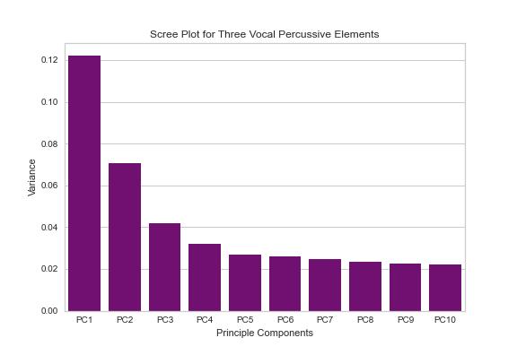
The following feature handling steps were selected according to the work of Stowell, 2010 with reference to engineering audio features for QBV. Following extraction, features were either standardised to have a mean of 0 and a standard deviation of 1 or normalised between 0 - 1 across all vocal percussive elements. The scaled feature vector was then reduced in dimensionality via a dimensionality reduction technique. PCA has been the most widely used data reduction technique during this work but other options for dimension reduction were explored, including Factor Analysis (FA) and Independent Component Analysis (ICA). PCA is employed in this project as a method of dimensionality reduction to reveal principle components (PC). These are latent axes that best represent the variance of the data (fig 8). Number of components (i.e., the number of dimensions to reduce to) was chosen through a combination of manual hyperparameter testing, scree plot analysis,and automated hyperparameter tuning (this process is described at length in chapter 3.10). A scree plot (fig 7) demonstrates how much of the feature set’s variance is captured by each PC in the principle subspace. This can assist with the selection of an appropriate value for number of components when creating a PCA model.

Figure 7. Scree Plot for three_perc Dataset Principle Components 1−10 The first PC will always capture the highest percentage of the data’s variance and as the number of PC increases the amount of variance each PC represents decreases. PCA is often used in combination with clustering to reduce a higher-dimensional feature set to a lower-dimensional representation,often giving a better visual segmentation of classes described by a set of audio features (Baniya, Joonwhoan Lee and Ze-Nian Li, 2014).

It can be seen in (fig 7) that the contribution of the principle components becomes linear at around ���� = 5, this, combined with the results presented in chapter 4 (table III) for hyperparameter tuning of number of dimensions determines five to be an ideal number of PCs to capture the variance of the data. The following stage in the pipeline implementation allows both feature scaling and dimensionality reduction.

Fig 8. An Example of a Feature Set Before (top) and After Principle Component Analysis (bottom)

The FeatureHandling class has two significant methods. These are _scale_features and _get_reduction. This allows the user to specify scaling type, with a choice between standardisation and normalisation. A user may also specify the dimensionality reduction technique and the number of dimensions to which they wish to reduce the feature set. The input feature set, target number of dimensions, dimensionality reduction type, and scaling type are passed as parameters to the FeatureHandling constructor upon object creation. In the case that ������������������������������������ > 3 it is not possible to visualise the dimensions that exceed the third. If the output of a higher dimensional principle subspace is visualised it will be limited to a two-dimensional visualisation (fig 9), or threedimensional visualisation with a 3D plot (fig 10).

Figure 9. Clustering Visualised on a Two-Dimensional Principle Subspace