Nikolaos Apeiranthitis, Lorenza Sardisco, Johanna Tepsell: Characterization of unconventional lithium deposits - A case study using XRD, ICP-MS/OES and LIBS for quantitative Li analysis

Introduction

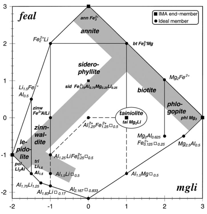
Lithium is in great demand in the battery mineral sector working as one of the key metals enabling the renewable energy transition. Recently, Li has been added to the EU list of Critical Raw Materials as the EU is dependent on exports to satisfy existing, not-withstanding future demand. Renewed exploration strategies and analytical techniques are required to discover new Li sources. Traditionally, Li exploration has been focused on spodumene-bearing pegmatite and Li-brines but additional secure sources will be needed to match the future demand. Along with spodumene, lithium-bearing micas are among the most economic and common Li-minerals together with petalite, hectorite, jadarite, amblygonite and eucryptite. They occur in evolved granites and related pegmatite and aplites presenting a compelling alternative Li source. Lithium-bearing micas are true trioctahedral micas and comprise the mineral series lepidolite and zinnwaldite, and the minerals trililithionite, polylithionite, masutomilite, tainiolite, norrishite and ephesite, Figure 1. There is also a composition series between lithian muscovite and lepidolite and consequent dioctahedral to trioctahedral mica transition (Fleet, 2005; Rieder, 1999).

Potassium micas representation. The red triangle includes lithium-bearing micas of interest, such as zinnwaldite and lepidolite. X-axis is ‘mgli’ (Mg - Li) content while the y-axis is the ‘feal’ (Fetot+Mg+Ti -IVAl) content. Modified after Tischendorf et al. (2004).

Figure 2. XRD quantification results of the 25 Cornish granite samples characterised for their lithium-bearing mica content and overall mineralogy.

Figure 3. XRD diffraction patterns of sample JD13-DY14 at selected angles (5° to 50° 20).

Lithium content in lithium-bearing mica is very variable: from 3,42% for median zinnwaldite to 5,39% Li2O for median lepidolite (Tischendorf et al., 2001) up to 6,97 in polylithionite (Cerny & Trueman, 1985), while lithian muscovite could host up to 3,3% of Li2O without changing its structure (Levinson, 1952).

As a part of an extensive research and development project, “Quantifying unconventional lithium resource potential with novel rapid in-situ analyses”, more than 150 samples from different UK locations have been analysed in order to set up a bespoke workflow for the characterization of unconventional lithium-bearing minerals and their associated host rocks. The utilized analytical techniques include X-ray Diffraction (XRD), and Laser-Induced Breakdown Spectroscopy (LIBS) among other techniques. Selected results of these studies are described below with emphasis on quantitative analysis of lithium-bearing micas and quantification of Li in Li-bearing rocks using statistical models. The samples used for these studies were collected from Cornish granites with lithium-bearing mica (XRD, ICP-MS/OES) and from an abandoned Fe-Mn mine with secondary Li-bearing manganese minerals (LIBS).

Identification and quantification of lithium-bearing micas by XRD

XRD analysis was conducted at X-ray Mineral Services Ltd, UK, using a PANalytical X’Pert3 diffractometer. The samples were analysed using HighScore Plus by PANalytical and quantified using the Rietveld method with BGMN AutoQuan software.

In Figure 2, the XRD results are shown for each of the Cornish samples analysed. The Cornish granite samples contain four types of mica: biotite, muscovite, lepidolite and zinnwaldite. The distinction of different micas by XRD is challenging as all the micas share their main reflection at the same 2θ position in the diffraction pattern. Only an accurate study of the ratio between the mica reflections and precise calculation of their positions can help in the differentiation of the mica species. A mass balance calculation has been used to assess the quality of the mineral’s quantification given by the Rietveld method and to confirm mica specification. Simplified mineral formulas have been used to calculate the bulk chemical composition of the samples from the quantification of the minerals obtained by the XRD method. This calculated bulk chemical composition was compared with the measured chemical composition obtained with ICP-OES/MS analysis. The scope of the mass balance calculation is to identify a mismatch between the chemical composition of a sample and its mineral content. In most samples, there is a good correlation between the calculated chemistry and the measured one showing the accuracy of the XRD mineral quantification and confirming the ability of XRD to distinguish and quantify lithium-bearing micas even when both zinnwaldite and lepidolite are present in the same sample as in sample JD13-DY14 (Figure 3).

Figure 4. Lithium versus trace elements cross plots with high R2 score, within the mica-rich granitic samples

Figure 5. A linear model investigation of different train/test splits for model representativity analysis and model selection for Li quantification. The root mean square error (RMSE) of cross-validation and prediction, as well as the R2 coefficient for both cross-validation and prediction, are monitored over the different train/test splits

Quantification of Li using pathfinder elements in granitic rocks

The same set of Cornish granite samples and a lepidolite crystal were analysed with ICP-MS/OES to acquire a full trace elements fingerprint as well as Li quantification. These data were used to produce a model which would predict Li concentrations using pathfinder elements associated with the micas present such as zinnwaldite and lepidolite as demonstrated in the previous section and Figure 2.

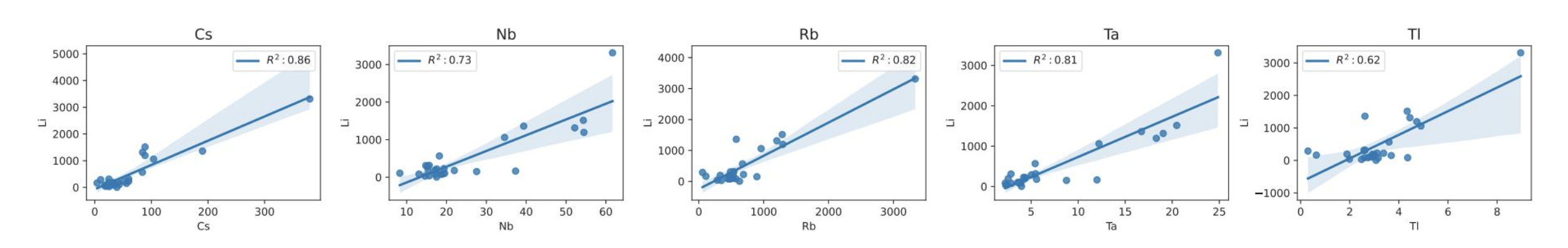
The Li ICP-OES/MS concentration in the analysed samples shows a range of 4–3311 ppm, which gives us the ability to produce a first representative model. A data exploratory step was performed, by creating Li vs trace element cross plots, in order to assess, which trace elements correlate linearly with Li. This process resulted that Cs, Nb, Rb, Ta and Tl had the highest R2 correlation coefficient of 0,86, 0,73, 0,82, 0,81, and 0,62, respectively, when plotted against Li, as shown in Figure 4.

Following that and in order to produce a robust predictive model, the data was split in an 80:20 fashion for model training and testing, respectively. In the first instance, 10 splits were made using the Kennard Stone algorithm (Kennard & Stone, 1969) making the modelling process more appropriate for geochemistry applications. For each split, a linear model was fitted on the training split, performing a 5-fold cross-validation. Based on that, a predictive step was performed on the test split, for evaluating the predictive capability of the trained & cross-validated model. At the end of the 10 splits modelling, it was possible to evaluate the root mean square error of the 5-fold cross-validated model (RMSE - CV), and the RMSE of the prediction on test split (RMSE - P), as well as the R2 of both the 5-fold cross-validation (R2- CV) and the prediction of the test split (R2 – P), (Figure 5).

It can be seen that each of the 10 trained models has a different predictive capability. For example, for Split 4 the R2 -P is at 0,98 with a range of test Li concentration at 100–1200 ppm, while for split 5 the R2-P is at -3,72 for a test Li concentration at 100–350 ppm. However, across the 10 splits trained and tested, 50% of the time a high R2-P scoring model can be produced with an error of <200 ppm (based on the RMSE -P), (Figure 5).

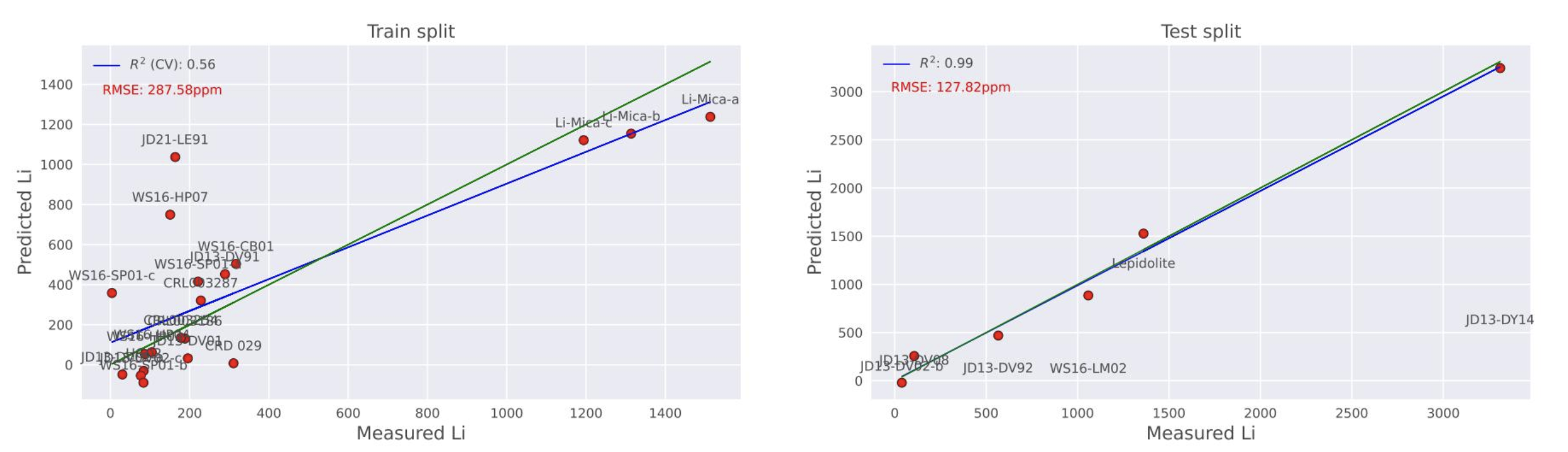
Upon further investigation, a final model was devised which allowed us to uncover, qualitatively, the presence of outlier samples which can inhibit predictive capability. In this final model, the test split was arranged across the full range of Li concentration in our data set, including the highest Li-bearing sample (Figure 6). In Figure 7, it can be seen that while the training R2 value has a relatively low scoring (0,56) due to the presence of samples JD21-LE91 and WS16-HP07, the R2 of the prediction is at R2=0,99, with a RMSE of 128 ppm. It’s interesting that the highest Li concentration is predicted very well, despite the fact that the trained model is extrapolated to predict this high value.

In conclusion, it can be said that this first model gave us a good insight on

• The pathfinder elements strongly associated with Li when zinnwaldite and lepidolite are hosted within granites

• The robustness of multivariate linear modelling can exhibit for modelling

Li concentration based on the above elements

This work is on-going and the next part of this study is to feed this trained model with portable-based XRF analysis of the pathfinder elements, to evaluate its predictive capacity and accuracy on Li concentration predicted.

Figure 6. Final model train and test splits population (left) and trace elements graph of the different train/test samples (right)

Figure 7. The train split cross-validation (left) and test split prediction (right) of Li as devised for the final Li quantification model using geochemical data. Outlier samples are included in the back circle for the training split.

Figure 8. Partial least square regression model investigation of different train/test splits for model representativity analysis and model selection for Li quantification by LIBS. The root mean square error (RMSE) of cross-validation and prediction, as well as the R2 coefficient for both cross-validation and prediction, are monitored over the different train/test splits.

Lithium quantification in Li-bearing rocks and spodumene mixes with Laser Induced Breakdown Spectroscopy (LIBS) analysis

As LIBS technology has resurfaced the recent years, it has shown great interest in mining exploration campaigns. One of its strong characteristics is the detection of Li, a light element, which is unquantifiable by traditional techniques such as X-ray Fluorescence (XRF) analysis or needs a lot of sample preparation when analysed utilizing a 4-acid digestion method with an ICP-OES/ MS finish. With LIBS technology and upon appropriate sample representation, LIBS spectra can be acquired and along with ICP analysis, quantification models can be built for different rock matrices, which can provide cost-effective Li data for faster decision-making during Li exploration campaigns. In the following example, a first model of ICP -LIBS Li quantification is presented. The model is based on a series of samples hosting Li-bearing manganese oxides collected from Wales (UK) together with a set of spodumene mixes with plagioclase and quartz. The spodumene used for creating these mixes is a spodumene crystal extensive-

ly characterised by XRD, ICP-MS/OES and FTIR methods with the results published in (Sardisco et al., 2022). The manganese oxide samples provided a Li concentration range of 4–3488 ppm, while the spodumene mixes provided a range of 4–24863 ppm.

Figure 9. Train/test split sample population and Li LIBS spectra of the best-fitted model

Figure 10. The train split cross-validation (left) and test split prediction (right) of Li as devised for the final Li quantification model of LIBS spectra

An exploratory analysis of different train/ test splits, as described in the previous modelling example, was also performed revealing the error and the predictive capability of each trained model for each train/test split, as shown in Figure 8. For this ICP-LIBS model, a partial least square regression model was performed as it has been shown to be more appropriate for modelling spectroscopic data (Clegg et al., 2009; Krüger et al., 2020).

It can be seen that although the R2 of the prediction score is very high (0,7 or 0,9) for all splits models, apart from split 8 and split 10, the root mean square error RMSE (P) has a higher value for splits 4, 5, 8, 9, 10 than RMSE (CV). This is an indication that this specific train/test partitioning of samples doesn’t provide a sufficient generalisation of the data set. So, tracking how the error changes between the train (cross-validation) and the test predictions is an important modelling parameter.

The final model was selected for the data above, and is presented in Figure 9 and Figure 10. The training split gave a very good R2 score of 0,922 with a relatively high RMSE at 2093 ppm. The test split, although it represented half the concentration range of Li in these samples, gave a very good R2 score of 0,97 with an RMSE of 852 ppm, Figure 10.

It can be concluded that the final model presented for ICP-LIBS Li quantification has relatively high training and predictive error, although the R2 is very high, which needs further investigation for improvement. However, it is a good demonstration of how ICP-MS/OES and LIBS data can be combined for acquiring Li quantification with less sample preparation and faster turn-around.

Conclusions

This project was designed to develop new analytical workflows to optimise the analysis of Li and the characterisation of Li-bearing minerals and their associated host rocks with an emphasis on unconventional Li-phases and statistical modelling. In the three examples explained above, the capabilities of XRD, ICP-MS/OES and LIBS analytical techniques for the characterization of unconventional Li deposits have been demonstrated. These techniques can be used for the identification and quantification of Li-bearing minerals in various rock matrices. High-quality XRD analysis provides an accurate quantification of various Li-minerals including lithium-bearing micas such as zinnwaldite and lepidolite, which have traditionally been challenging to differentiate from each other because of their similar spectral patterns. While Li data can be acquired accurately using 4 acid digestion with an ICP-MS/ OES finish, the use of statistical modelling of these data can provide an additional fast Li quantification tool in conjunction with portable/hand-held techniques such as XRF and LIBS. ▲

References

Cerny, P., & Trueman, D. (1985). Polylithionite from the rare-metal deposits of the Blachford Lake alkaline complex. American Mineralogist, 70, 1127–1134.

Clegg, S. M., Sklute, E., Dyar, M. D., Barefield, J. E., & Wiens, R. C. (2009). Multivariate analysis of remote laser-induced breakdown spectroscopy spectra using partial least squares, principal component analysis, and related techniques. Spectrochimica Acta - Part B AtomicSpectroscopy,64(1), 79–88. https:// doi.org/10.1016/j.sab.2008.10.045

Fleet, M. E. (2005). Rock-forming minerals. Vol 3A: Micas (M. E. Fleet, Ed.; 2nd ed.). Geological Society.

Kennard, R. W., & Stone, L. A. (1969). Computer Aided Design of Experiments. Technometrics, 11(1), 137–148.

Krüger, A. L., Nicolodelli, G., Villas-Boas, P. R., Watanabe, A., & Milori, D. M. B. P. (2020). Quantitative Multi-Element Analysis in Soil Using 532 nm and 1064 nm Lasers in LIBS Technique. Plasma Chemistry and Plasma Processing, 40(6), 1417–1427. https://doi. org/10.1007/s11090-020-10116-9

Levinson, A. A. (1952). Studies in the mica group; relationship between polymorphism and composition in the muscovite-lepidolite series. University of Michigan.

Rieder, M. (1999). Nomenclature of the Micas. Mineralogical Magazine, 63(2), 267–279. https://doi.org/10.1180/002646199548385

Sardisco, L., Hannula, P. M., Pearce, T. J., & Morgan, L. (2022). Multi-Technique Analytical Approach to Quantitative Analysis of Spodumene. Minerals, 12(2). https://doi. org/10.3390/min12020175

Tischendorf, G., Förster, H.-J., & Gottesmann, B. (2001). Minor- and trace-element composition of trioctahedral micas: a review. Mineralogical Magazine, 65(2), 249–276. https://doi. org/10.1180/002646101550244

Tischendorf, G., Rieder, M., Förster, H.-J., Gottesmann, B., & Guidotti, Ch. V. (2004). A new graphical presentation and subdivision of potassium micas. Mineralogical Magazine, 68(4), 649–667. https://doi. org/10.1180/0026461046840210

TEXT: NIKOLAOS APEIRANTHITIS1, LORENZA SARDISCO1, JOHANNA TEPSELL2