USING POROSITY OF EPITAXIAL LAYER TO DECREASE QUANTITY OF RADIATION DEFECTS GENERATED DURING RADIATI by journalmsej

Advances in Materials Science and Engineering: An International Journal (MSEJ), Vol. 3, No. 2, June 2016

USING POROSITY OF EPITAXIAL LAYER TO DECREASE QUANTITY OF RADIATION DEFECTS GENERATED DURING RADIATION PROCESSING OF A MULTILAYER STRUCTURE E.L. Pankratov1, E.A. Bulaeva1,2 1

Nizhny Novgorod State University, 23 Gagarin avenue, Nizhny Novgorod, 603950, Russia 2 Nizhny Novgorod State University of Architecture and Civil Engineering, 65 Il'insky street, Nizhny Novgorod, 603950, Russia

ABSTRACT In this paper we consider redistribution of radiation defects, which were generated during radiation processing, in a multilayer structure with porous epitaxial layer. It has been shown, that porosity of epitaxial layer gives a possibility to decrease quantity of radiation defects.

KEYWORDS Multilayer structure; porous epitaxial layer; radiation processing; decreasing of quantity of radiation defects.

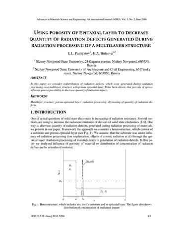
1. INTRODUCTION One of actual questions of solid state electronics is increasing of radiation resistance. Several methods are using to increase the radiation resistance of devices of solid state electronics [1-5]. One way to decrease quantity of radiation defects, generated during radiation processing of materials, we present in our paper. Framework the approach we consider a heterostructure, which consist of a substrate and porous epitaxial layer (see Fig. 1). We assume, that the substrate was under influence of radiation processing (ion implantation, effects of cosmic radiation et al) through the epitaxial layer. Radiation processing of materials leads to generation of radiation defects. In this paper we analyzed influence of porosity of material on distribution of concentration of radiation defects in the considered material.

C(x,t=0) D1

D(x)

D2 P2 0

Fig. 1. Heterostructure, which includes into itself a substrate and an epitaxial layer. The figure also shows distribution of concentration of implanted dopant DOI:10.5121/msej.2016.3204

Advances in Materials Science and Engineering: An International Journal (MSEJ), Vol. 3, No. 2, June 2016

2. METHOD OF SOLUTION We solve our aim by analysis of distributions of concentrations of radiation defects in space and time in the considered heterostructure. We determine the above distributions by solving the following system of equations [6-11]

∂ I ( x, y , z , t ) ∂  ∂ I ( x, y , z , t )  ∂  ∂ I (x, y , z , t )  =  D I (x, y , z , T ) +  D I ( x, y , z , T ) + ∂t ∂ x ∂x ∂y  ∂ y  +

∂ I ( x, y , z , t )  ∂   D I ( x, y , z , T )  − k I ,V ( x, y, z , T ) I (x, y , z , t ) V ( x, y, z , t ) − k I , I ( x, y , z , T ) × ∂ z ∂ z 

× I 2 ( x, y, z, t ) +

∂  DI S ∂ µ 2 ( x, y, z, t )  ∂  DI S ∂ µ 2 (x, y, z, t )  ∂  DI S ∂ µ 2 ( x, y, z, t )   +  +   ∂ x V k T ∂x ∂y ∂z  ∂ y V k T  ∂ z V k T 

∂ V ( x, y , z , t ) ∂  ∂ V ( x, y , z , t )  ∂  ∂ V ( x, y , z , t )  = DV (x, y, z , T ) +  DV ( x, y , z , T ) + ∂t ∂ x  ∂x ∂ y ∂y    +

(1)

∂ V ( x, y , z , t )  ∂   DV ( x, y, z , T )  − k I ,V (x, y , z , T ) I ( x, y, z , t ) V ( x, y , z , t ) − k V ,V ( x, y , z , T ) × ∂ z ∂ z 

× V 2 ( x, y, z, t ) +

∂  DV S ∂ µ 2 (x, y, z, t )  ∂  DV S ∂ µ 2 ( x, y, z, t )  ∂  DV S ∂ µ 2 (x, y, z, t )   +  +   ∂ x V k T ∂x ∂y ∂z  ∂ y V k T  ∂ z V k T 

with boundary and initial conditions

∂ I ( x, y , z , t ) ∂ I (x, y, z, t ) ∂ I ( x, y , z , t ) ∂ I ( x, y , z , t ) = 0, = 0, =0, =0, ∂y ∂y ∂x ∂x y =0 y=Ly x =0 x =Lx ∂ V (x, y, z, t ) ∂ I ( x, y , z , t ) ∂ V ( x, y , z , t ) ∂ I ( x, y , z , t ) = 0, = 0, =0, =0, ∂z ∂z ∂x ∂x z =0 z = Lz x=0 x=Lx ∂ V (x, y, z, t ) ∂ V (x, y, z, t ) ∂ V ( x, y , z , t ) ∂ V (x, y, z, t ) = 0, =0, =0, =0, ∂y ∂ y ∂ z ∂z y =0 y=Ly z =0 z = Lz  2 lω I (x,y,z,0)=fI (x,y,z), V (x,y,z,0)=fV (x,y,z), V ( x1 + Vnt, y1 + Vnt, z1 +Vnt, t ) = V * 1+  k T x2 + y2 + z 2 1 1 1 

  . (2)  

Here I (x,y,z,t) and V (x,y,z,t) are the spatio-temporal distributions of concentrations of interstitials and vacancies; I* and V* are the equilibrium distributions of concentrations of interstitials and vacancies; diffusion coefficients of interstitials and vacancies have been described by the following functions DI(x,y,z,T) and DV(x,y,z,T); terms with squares of concentrations of interstitials and vacancies (V2(x,y,z,t) and I2(x,y,z,t), respectively) correspond to generation divacancies and analogous complexes of interstitials (see, for example, [10] and appropriate references in this work); kI,V(x,y,z,T) is the parameter of recombination of point defects; kI,I(x,y,z,T) and kV,V(x,y,z,T) are the parameters of generation of complexes of point defects and generation; k, V*, l and a are the Boltzmann constant, the equilibrium distribution of vacancies, the atomic spacing and the specific surface energy, respectively. ω = a3. Framework taking into account porosity we assume, that at initial stage porous are approximately cylindrical with average dimensions r = x12 + y12 and z1 [12]. With time small pores decomposing into vacancies. The vacancies are absorbed by large pores [8]. The large pores takes spherical form during the absorbtion [8]. We determine distribu44

Advances in Materials Science and Engineering: An International Journal (MSEJ), Vol. 3, No. 2, June 2016

tion of concentration of vacancies, which was formed due to porosity, by summing over all pores, i.e. l

V ( x, y , z , t ) = ∑ ∑ ∑ V p ( x + i α , y + j β , z + k χ , t ) , R = x 2 + y 2 + z 2 . i = 0 j =0 k =0

Averaged distances between centers of pores are equal to α, β and χ in x, y and z directions, respectively. Quantities of pores in x, y and z directions are equal to i, j and k. Distributions of concentrations of divacancies ΦV(x,y,z,t) and diinterstitials ΦI (x,y,z,t) in space and time have been calculated by solving the following system of equations [9-11]

∂ Φ I (x, y, z, t ) ∂  ∂ Φ I (x, y, z, t )  ∂  ∂ Φ I (x, y, z, t )  =  DΦ I (x, y, z, T ) +  DΦ I (x, y, z, T ) + ∂t ∂x ∂x ∂y  ∂y  +

∂ Φ I ( x, y, z, t )  ∂  2  DΦ I (x, y, z, T )  + k I (x, y, z, T ) I ( x, y, z, t ) + k I ,I ( x, y, z, T ) I (x, y, z, t ) + ∂z ∂z  +

∂  DΦ I S ∂ µ 2 ( x, y , z , t )  ∂  DΦ I S ∂ µ 2 ( x, y, z , t )  ∂  DΦ I S ∂ µ 2 (x, y , z , t )   +  +   ∂ x V k T ∂x ∂y ∂z  ∂ y V k T  ∂ z V k T 

(3)

∂ ΦV (x, y, z, t ) ∂  ∂ ΦV (x, y, z, t )  ∂  ∂ ΦV (x, y, z, t )  =  DΦV (x, y, z,T ) + DΦV (x, y, z,T ) + ∂t ∂x ∂x ∂y  ∂y  +

∂ ΦV ( x, y, z, t )  ∂  2 DΦV (x, y, z,T )  + kV (x, y, z,T ) V ( x, y, z, t ) + kV ,V (x, y, z,T )V ( x, y, z, t ) + ∂z ∂z  +

∂  DΦV S ∂ µ 2 ( x, y , z , t )  ∂  DΦV S ∂ µ 2 ( x, y, z , t )  ∂  DΦV S ∂ µ 2 (x, y , z , t )   +  +   ∂ x V k T ∂x ∂y ∂z  ∂ y V k T  ∂ z V k T 

with boundary and initial conditions

∂ I (x, y, z,t ) ∂ Φ I (x, y, z, t ) ∂ I (x, y, z, t ) ∂ I (x, y, z, t ) = 0, =0, = 0, = 0, ∂x ∂ x ∂ y ∂y x =0 x= Lx y=0 y=Ly ∂ ΦI (x, y, z, t ) ∂ ΦV (x, y, z, t ) ∂ I (x, y, z, t ) ∂ V (x, y, z, t ) =0, = 0, = 0, = 0, ∂z ∂ z ∂ x ∂x z =0 z =Lz x =0 x=Lx

∂ ΦV (x, y, z, t ) ∂ V (x, y, z, t ) ∂ V (x, y, z, t ) ∂ V (x, y, z, t ) = 0, = 0, = 0, =0, ∂y ∂y ∂z ∂z y=0 y =L y z =0 z =Lz ΦI (x,y,z,0)=fΦI (x,y,z), ΦV (x,y,z,0)=fΦV (x,y,z).

(4)

Functions DΦI(x,y,z,T) and DΦV(x,y,z,T) describe spatial and temperature dependences of the diffusion coefficients of complexes of radiation defects; kI(x,y,z,T) and kV(x,y,z,T) are the parameters of decay of the above complexes. We calculate distributions of concentrations of radiation defects in space and time by method of averaging of function corrections [13]. To use the approach we write the Eqs. (1) and (3) with account initial distributions of defects, i.e.

Advances in Materials Science and Engineering: An International Journal (MSEJ), Vol. 3, No. 2, June 2016

∂ I ( x, y , z , t ) ∂  ∂ I ( x, y , z , t )  ∂  ∂ I ( x, y , z , t )  =  D I ( x, y , z , T ) +  D I ( x, y , z , T ) + ∂t ∂ x ∂x ∂y  ∂ y  +

∂ I ( x, y , z , t )  ∂  DI ( x, y, z, T )  − k I ,V (x, y, z , T ) I (x, y, z , t )V ( x, y, z, t ) + f I ( x, y, z )δ (t ) + ∂ z  ∂ z  +

∂  DI S ∂ µ 2 ( x, y , z , t )  ∂  DI S ∂ µ 2 ( x, y , z , t )  ∂  D I S ∂ µ 2 ( x, y , z , t )   +  +  − ∂ x V k T ∂x ∂y ∂z  ∂ y V k T  ∂ z V k T 

− k I , I ( x, y , z , T ) I 2 ( x , y , z , t ) (1a)

∂ V ( x, y , z , t ) ∂  ∂ V ( x, y , z , t )  ∂  ∂ V ( x, y , z , t )  =  DV (x, y, z , T ) +  DV ( x, y , z , T ) + ∂t ∂ x ∂x ∂y  ∂ y  +

∂  ∂ V (x, y , z , t )   DV (x, y , z , T )  − k I ,V (x, T ) I ( x, y , z , t )V ( x, y, z , t ) + f V ( x, y, z )δ (t ) + ∂ z ∂z 

∂  DV S ∂ µ 2 (x, y , z , t )  ∂  DV S ∂ µ 2 ( x, y , z , t )  ∂  DV S ∂ µ 2 ( x, y, z , t )   +  +  − ∂ x V k T ∂x ∂y ∂z  ∂ y V k T  ∂ z V k T 

− kV ,V ( x, y, z, T )V 2 ( x, y, z , t )

∂ Φ I ( x, y , z , t ) ∂  ∂ Φ I ( x, y , z , t )  ∂  ∂ Φ I ( x, y, z , t )  =  DΦI ( x, y, z, T ) +  DΦI (x, y, z, T ) + ∂t ∂x ∂x ∂y  ∂y  +

∂ Φ I (x, y, z, t )  ∂  2  DΦ I (x, y, z, T )  + k I (x, y, z, T ) I (x, y, z, t ) + k I , I ( x, y, z, T ) I ( x, y, z, t ) + ∂z ∂z  +

∂  DΦV S ∂ µ 2 ( x, y, z , t )  ∂  DΦV S ∂ µ 2 (x, y , z , t )  ∂  DΦV S ∂ µ 2 ( x, y, z , t )   +  +  + ∂ x V k T ∂x ∂y ∂z  ∂ y V k T  ∂ z V k T 

+ f Φ I ( x, y , z )δ (t ) (3a)

∂ ΦV (x, y, z, t ) ∂  ∂ ΦV (x, y, z, t )  ∂  ∂ ΦV (x, y, z, t ) = D (x, y, z, T ) +  DΦV (x, y, z, T ) + ∂t ∂ x  ΦV ∂x ∂ y ∂y    +

∂ ΦV ( x, y, z, t )  ∂  2 DΦV ( x, y, z, T )  + kV ( x, y, z, T ) V ( x, y, z, t ) + kV ,V ( x, y, z, T )V ( x, y, z, t ) + ∂ z  ∂z 

+ f Φ I ( x, y, z )δ (t ) . Now we use not yet known average values α1ρ of the required concentrations in right sides of the Eqs. (1a) and (3a) instead of the concentrations. The replacement gives us possibility to obtain following equations for determination the first-order approximations of concentrations of radiation defects in the following form

∂ I 1 ( x, y , z , t ) ∂  DI S ∂ µ 2 ( x, y , z , t )  ∂  DI S ∂ µ 2 ( x, y , z , t )  =  +   + f I (x, y , z )δ (t ) + ∂ x V k T ∂x ∂y ∂t  ∂ y V k T 

Advances in Materials Science and Engineering: An International Journal (MSEJ), Vol. 3, No. 2, June 2016

∂  DI S ∂ µ 2 ( x, y , z , t )  2   − α 1I k I , I (x, y, z , T ) − α 1I α 1V k I ,V ( x, y , z , T ) ∂ z V k T ∂z 

(1b)

∂ V1 (x, y, z , t ) ∂  DV S ∂ µ 2 (x, y, z , t )  ∂  DV S ∂ µ 2 (x, y, z , t )  =  +   + fV (x, y, z )δ (t ) + ∂ x V k T ∂x ∂y ∂t  ∂ y V k T  D ∂  V S ∂ µ 2 ( x, y , z , t )  2 +   − α 1V kV ,V (x, y , z , T ) − α 1I α 1V k I ,V ( x, y, z , T ) ∂ z V k T ∂z  ∂ Φ1I ( x, y, z, t ) ∂  DΦ I S ∂ µ 2 ( x, y, z, t )  ∂  DΦ I S ∂ µ 2 ( x, y, z, t )  =  +   + f Φ I (x, y, z )δ (t ) + ∂ x V k T ∂x ∂y ∂t  ∂ y V k T  +

∂  DΦ I S ∂ µ 2 ( x, y, z, t )  2   + k I ( x, y , z , T ) I ( x , y , z , t ) + k I , I ( x, y , z , T ) I ( x, y , z , t ) ∂ z V k T ∂z 

(3b)

∂ Φ1V ( x, y, z, t ) ∂  DΦV S ∂ µ 2 (x, y, z, t )  ∂  DΦV S ∂ µ 2 (x, y, z, t )  =  +   + f ΦV (x, y, z )δ (t ) + ∂ x V k T ∂x ∂y ∂t  ∂ y V k T  +

∂  DΦV S ∂ µ 2 ( x, y, z, t )  2   + kV ( x, y, z , T )V ( x, y, z, t ) + kV ,V ( x, y, z , T )V ( x, y, z , t ) . ∂ z V k T ∂z 

Integration of the both sides of Eqs. (1b) and (3b) on time gives a possibility to obtain first- order approximations of concentrations of radiation defects in the final form I 1 ( x, y , z , t ) =

t t ∂ t D I S ∂ µ 2 ( x, y , z , t ) d τ − α 12I ∫ k I , I (x, y, z, T ) d τ − α 1I α 1V ∫ k I ,V ( x, y, z , T ) d τ ∫ ∂ z 0V kT ∂z 0 0

V1 (x, y, z , t ) =

∂ t D I S ∂ µ 2 ( x, y , z , t ) ∂ t D I S ∂ µ 2 ( x, y , z , t ) dτ + d τ + f I ( x, y , z ) + ∫ ∫ ∂ x 0V kT ∂x ∂ y 0V kT ∂y

(1c)

∂ t DV S ∂ µ 2 (x, y, z , t ) ∂ t DV S ∂ µ 2 ( x, y, z , t ) dτ + d τ + f V ( x, y, z ) + ∫ ∫ ∂ x 0V kT ∂x ∂ y 0V kT ∂y

t t ∂ t DV S ∂ µ 2 (x, y, z, t ) d τ − α 12V ∫ kV ,V (x, y, z , T ) d τ − α 1I α 1V ∫ k I ,V ( x, y, z , T ) d τ ∫ ∂ z 0V kT ∂z 0 0

Φ1I ( x, y, z, t ) = f Φ I (x, y, z ) + ∫ k I (x, y, z,T ) I ( x, y, z,τ ) d τ + ∫ k I ,I (x, y, z,T ) I 2 (x, y, z,τ ) d τ +

∂ t DΦ S ∂ µ2 (x, y, z,τ ) ∂ t DΦI S ∂ µ2 (x, y, z,τ ) ∂ t DΦ S ∂ µ2 (x, y, z,τ ) + ∫ I dτ + dτ + ∫ I dτ ∫ ∂ x 0 V kT ∂x ∂ y 0V kT ∂y ∂ z 0 V kT ∂z +

∂ t DΦI S ∂ µ2 (x, y, z,τ ) ∂ t DΦI S ∂ µ2 (x, y, z,τ ) ∂ t DΦ S ∂ µ2 (x, y, z,τ ) dτ + dτ + ∫ I dτ ∫ ∫ ∂ x 0 V kT ∂x ∂ y 0V kT ∂y ∂ z 0 V kT ∂z t

(3c)

Φ1V (x, y, z, t ) = f ΦV (x, y, z ) + ∫ kV (x, y, z, T )V (x, y, z,τ ) d τ + ∫ kV ,V (x, y, z, T )V 2 (x, y, z,τ ) d τ + 0

∂ DΦV S ∂ µ 2 (x, y, z,τ ) ∂ DΦV S ∂ µ2 (x, y, z,τ ) ∂ t DΦV S ∂ µ 2 (x, y, z,τ ) dτ + dτ + dτ . ∫ ∫ ∫ ∂ x 0V kT ∂x ∂ y 0V kT ∂y ∂ z 0V kT ∂z t

We calculate average values of the required approximations by the following relation [13] 47

Advances in Materials Science and Engineering: An International Journal (MSEJ), Vol. 3, No. 2, June 2016

α 1ρ =

Θ Lx L y Lz 1 ∫ ∫ ∫ ∫ ρ 1 ( x, y , z , t ) d z d y d x d t . ΘLx L y Lz 0 0 0 0

(5)

Substitution of the relations (1c) and (3c) into the relation (5) gives a possibility to calculate the required average values in the following form

(a3 + A)2 − 4  B + Θ a3 B + Θ 2 Lx L y Lz a1  − a3 + A , α

α1I = ×

 

4 a 42

 

4 a4

 Lx L y L z =  ∫ ∫ ∫ f I (x, y , z ) d z d y d x × 0 0 0

Lx L y Lz  1 RI1 1 − α 1I S II 00 − Θ L x L y L z  , α 1Φ I = + ∫ ∫ ∫ f Φ ( x, y , z ) d z d y d x + ΘL x L y L z L x L y L z 0 0 0 I  S IV 00 RV 1 + SVV 20 S II 20 1 Lx L y Lz , α1ΦV = . + ∫ ∫ ∫ f ΦV (x, y, z ) d z d y d x + ΘL x L y L z L x L y Lz 0 0 0 ΘLx L y Lz

α 1I

Lx Ly Lz

0 0 0

(

)

Here Sρρ ij = ∫ (Θ − t ) ∫ ∫ ∫ kρ ,ρ ( x, y, z,T ) I1i ( x, y, z, t )V1 j ( x, y, z, t ) d z d y d x d t , a4 = S IV2 00 − S II 00 SVV 00 × L x L y Lz

× S II 00 , a3 = S IV 00 S II 00 + S IV2 00 − S II 00 SVV 00 , a 2 = S IV 00 S IV2 00 ∫ ∫ ∫ f V (x, y , z ) d z d y d x + 2 S VV 00 × 0 0 L x L y Lz

Lx L y Lz

× S II 00 ∫ ∫ ∫ f I (x, y, z ) d z d y d x − S IV2 00 ∫ ∫ ∫ f I (x, y, z ) d z d y d x + S IV 00 ΘL2x L2y L2z − L2x L2y L2z × 0 0

× Θ SVV 00 , a1 = S IV 00

0 0

0 2

Θ 3 a2 Lx Ly Lz  × ∫ ∫ ∫ f I (x, y, z ) d z d y d x , a0 = SVV 00  ∫ ∫ ∫ f I (x, y, z ) d z d y d x , q = 24 a 42 0 0 0 0 0 0 

Lx L y Lz

4 2 2  a 2  Θ3 a23 a 2 2 2 Θ a1 2 a3  4 Θ a2 − Θ2 3  − − L L L , A = 8 y + Θ − 4Θ 2 , x y z 3 2 2 a 54 a 8 a a a4 4  4 4 4  L Lx y Lz Θ 4a a Θ a1 a 3 Θ a2 − Lx L y Lz , Rρ i = ∫ (Θ − t ) ∫ ∫ ∫ k I (x, y, z, T ) I 1i (x, y, z, t ) d z d y d x d t , p = Θ 2 0 24 − 0 0 0 0 12 a 4 18 a 4 12 a 42 Θ a2 3 B= + q2 + p3 − q − 3 q 2 + p3 + q . 6 a4

 aa  a ×  4a0 − Θ Lx Ly Lz 1 3  − Θ2 02 a4  8a4 

Approximations of concentrations of radiations defects with the second and higher orders have been calculated framework standard iterative procedure of method of averaging of function corrections [13]. Framework the procedure we determine the approximation of the n-th order by replacement of the concentrations of radiation defects I (x,y,z, t), V (x,y,z,t), ΦI (x,y,z,t) and ΦV (x,y,z,t) in right sides of the Eqs.(1b) and (3b) on the following sums αnρ+ρ n-1(x,y,z,t). The replacement gives a possibility to obtain the second-order approximations of concentrations of radiation defects

∂ I 2 ( x, y , z , t ) ∂  ∂ I 1 ( x, y , z , t )  ∂  ∂ I 1 ( x, y , z , t )  =  D I ( x, y , z , T ) +  D I ( x, y , z , T ) + ∂t ∂ x ∂x ∂y  ∂ y  ∂ I 1 (x, y , z , t )  ∂   DI ( x, y , z , T )  − k I ,V (x, y , z , T )[α 1 I + I 1 ( x, y , z , t )][α 1V + V1 ( x, y, z , t )]+ ∂ z ∂ z  ∂ t DI S ∂ µ2 ( x, y, z, t ) ∂ t DI S ∂ µ2 ( x, y, z, t ) ∂ t DI S ∂ µ2 (x, y, z, t ) + dτ + dτ + ∫ dτ − ∫ ∫ ∂ x 0V kT ∂x ∂ y 0V kT ∂y ∂ z 0V kT ∂z

− k I , I ( x, y, z , T ) [α 1I + I 1 ( x, y , z , t )]

(1d) 48

Advances in Materials Science and Engineering: An International Journal (MSEJ), Vol. 3, No. 2, June 2016

∂ V2 ( x, y, z, t ) ∂  ∂ V1 (x, y, z , t )  ∂  ∂ V1 ( x, y, z, t )  =  DV ( x, y, z , T ) +  DV (x, y, z , T ) + ∂t ∂ x ∂x ∂y  ∂ y  ∂ V ( x, y , z , t )  ∂  D (x, y, z , T ) 1  − k I ,V (x, y, z , T )[α 1I + I1 (x, y, z , t )][α 1V + V1 (x, y, z , t )]+ ∂ z  V ∂z  t D ∂ ∂ t DI S ∂ µ2 ( x, y, z, t ) ∂ t DI S ∂ µ2 (x, y, z, t ) I S ∂ µ 2 ( x, y, z, t ) + dτ + dτ + ∫ dτ − ∫ ∫ ∂ x 0V kT ∂x ∂ y 0V kT ∂y ∂ z 0V kT ∂z

− kV ,V ( x, y, z , T )[α 1I + V1 ( x, y, z , t )]

∂ Φ 2 I ( x, y, z, t ) ∂  ∂ Φ1I (x, y, z, t )  ∂  ∂ Φ1I ( x, y, z, t )  = DΦ I ( x, y, z, T ) + DΦ I ( x, y, z, T ) + ∂t ∂x ∂x ∂y  ∂y  +

∂ Φ1I (x, y, z, t )  ∂  2 DΦ I (x, y, z, T )  + k I , I (x, y, z, T ) I ( x, y, z, t ) + f Φ I (x, y, z )δ (t ) + k I (x, y, z, T ) × ∂ z ∂z  ∂  DΦ I S ∂ µ 2 ( x, y , z , t )  ∂  D Φ I S ∂ µ 2 ( x, y , z , t )  ∂  D Φ I S ∂ µ 2 ( x, y , z , t )   +  +   (3d) ∂ x V k T ∂x ∂y ∂z  ∂ y V k T  ∂ z V k T  ∂ Φ 2V (x, y, z, t ) ∂  ∂ Φ1V (x, y, z, t )  ∂  ∂ Φ1V (x, y, z, t )  D (x, y, z, T ) = + DΦV (x, y, z, T ) + ∂t ∂ x  ΦV ∂x ∂ y ∂y    +

∂ Φ 1 I ( x, y , z , t )  ∂  2  DΦV (x, y, z , T )  + k V ,V (x, y, z , T )V ( x, y, z , t ) + k V (x, y , z , T ) V (x, y , z , t ) + ∂ z ∂z  ∂  D ΦV S ∂ µ 2 ( x, y , z , t )  ∂  D ΦV S ∂ µ 2 ( x, y , z , t )  ∂  D ΦV S ∂ µ 2 ( x, y , z , t )   +  +  . ∂ x V k T ∂x ∂y ∂z  ∂ y V k T  ∂ z V k T 

Integration of the both sides of Eqs. (1d) and (3d) gives a possibility to obtain relations for the second-order approximations of the required concentrations of radiation defects in the following form

∂ I1 (x, y, z,τ ) ∂ I1 (x, y, z,τ ) ∂ t ∂ t dτ + dτ + ∫ D I ( x, y , z , T ) ∫ DI (x, y, z , T ) ∂x ∂ x0 ∂ y0 ∂y t ∂ I 1 ( x , y , z ,τ ) ∂ t 2 + d τ − ∫ k I , I (x, y , z , T ) [α 2 I + I 1 (x, y , z ,τ )] d τ − ∫ DI (x, y , z , T ) ∂ z0 ∂z 0

I 2 ( x, y , z , t ) =

− ∫ k I ,V ( x, y, z , T ) [α 2 I + I 1 ( x, y, z, τ )][α 2V + V1 ( x, y , z,τ )] d τ + f I (x, y , z ) + 0

∂  DI S ∂ µ 2 ( x, y , z , t )  ∂  D I S ∂ µ 2 ( x, y , z , t )  ∂  D I S ∂ µ 2 ( x, y , z , t )   +  +   ∂ x V k T ∂ x ∂ y ∂z  ∂ y V k T  ∂ z V k T 

∂  DI S ∂ µ 2 ( x, y , z , t )  ∂  D I S ∂ µ 2 ( x, y , z , t )  ∂  D I S ∂ µ 2 ( x, y , z , t )   +  +   (1e) ∂ x V k T ∂ x ∂ y ∂z  ∂ y V k T  ∂ z V k T  ∂ V1 (x, y, z,τ ) ∂ V1 ( x, y, z,τ ) ∂ t ∂ t dτ + dτ + ∫ DV ( x, y, z, T ) ∫ DV (x, y, z, T ) ∂x ∂ x0 ∂ y0 ∂y t ∂ V1 ( x, y , z ,τ ) ∂ t 2 + d τ − ∫ kV ,V ( x, y , z , T ) [α 2V + V1 ( x, y, z ,τ )] d τ − ∫ DV (x, y , z , T ) ∂ z0 ∂z 0

V2 (x, y, z, t ) =

− ∫ k I ,V (x, y , z , T )[α VI + I 1 (x, y , z ,τ )][α 2V + V1 (x, y , z ,τ )] d τ + fV (x, y , z ) + 0

Advances in Materials Science and Engineering: An International Journal (MSEJ), Vol. 3, No. 2, June 2016

∂  DV S ∂ µ 2 ( x, y, z , t )  ∂  DV S ∂ µ 2 ( x, y , z , t )  ∂  DV S ∂ µ 2 ( x, y , z , t )  +  +   ∂ x V k T ∂ x ∂ y ∂z  ∂ y V k T  ∂ z V k T  ∂ Φ1I (x, y, z,τ ) ∂ Φ1I (x, y, z,τ ) ∂ t ∂ t Φ 2 I (x, y, z, t ) = dτ + dτ + ∫ DΦ ( x, y, z, T ) ∫ DΦ (x, y, z, T ) ∂ x ∂ y ∂ x0 I ∂ y0 I t ∂ Φ 1 I ( x, y , z , τ ) ∂ t + d τ + ∫ k I , I ( x, y , z , T ) I 2 ( x, y , z , τ ) d τ + f Φ I ( x, y , z ) + ∫ D Φ I ( x, y , z , T ) ∂ z0 ∂ z 0 t t D D ∂ ∂ ∂ t DΦ I S ∂ µ 2 (x, y, z, τ ) Φ I S ∂ µ 2 ( x, y , z , τ ) Φ I S ∂ µ 2 ( x, y , z , τ ) + dτ + dτ + dτ + ∫ ∫ ∫ ∂ x 0V kT ∂x ∂ y 0V kT ∂y ∂ z 0V kT ∂z +

+ ∫ k I ( x, y , z , T ) I ( x, y , z , τ ) d τ

(3e)

∂ Φ 1V (x, y , z , τ ) ∂ t ∂ t d τ + f ΦV ( x , y , z ) + ∫ D ΦV ( x , y , z , T ) ∫ D Φ ( x, y , z , T ) + ∂ x0 ∂ x ∂ y0 V t ∂ Φ 1V (x, y, z, τ ) ∂ t + d τ + f ΦV ( x , y , z ) + ∫ k V ( x , y , z , T ) V ( x , y , z , τ ) d τ + ∫ D ΦV ( x , y , z , T ) ∂ z0 ∂ z 0 t t ∂ DΦ S ∂ µ2 (x, y, z,τ ) ∂ DΦV S ∂ µ2 ( x, y, z,τ ) ∂ t DΦ S ∂ µ2 ( x, y, z,τ ) + ∫ V dτ + dτ + ∫ V dτ + ∫ ∂ x 0V kT ∂x ∂ y 0V kT ∂y ∂ z 0 V kT ∂z

Φ 2V ( x, y, z , t ) =

+ ∫ kV ,V (x, y, z , T )V 2 ( x, y , z ,τ ) d τ . 0

We determine average values of the second-order approximations by the standard relation [13]

α 2ρ =

Θ L x L y Lz 1 ∫ ∫ ∫ ∫ [ρ 2 (x, y , z , t ) − ρ1 ( x, y, z , t )]d z d y d x d t . ΘLx L y Lz 0 0 0 0

(6)

Substitution of the relations (1e) and (3e) in the relation (6) gives a possibility to obtain relations for the required values α 2ρ

α2C=0, α2ΦI =0, α2ΦV =0, α 2V = α 2I =

where b4 =

(b3 + E )2 − 4  F + Θ a3 F + Θ 2 Lx L y Lz b1  − b3 + E , 4 b42

 

 

CV − α SVV 00 − α 2V (2 SVV 01 + S I V 10 + ΘLx L y Lz ) − SV V 02 − S I V 11 2 2V

S IV 01 + α 2V S IV 00

4 b4

S II 00 SVV 00 1 1 2 S IV2 00 SV V 00 − SVV + 00 S II 00 , b3 = −(2SVV 01 + S IV 10 + ΘLx L y Lz ) ΘLx Ly Lz ΘLx Ly Lz ΘLx Ly Lz

2 2 S IV 00 SVV 00 (S IV 01 + 2S II10 + S IV 01 + ΘLx Ly Lz ) + (2SVV 01 + S IV10 + ΘLx Ly Lz ) S IV 00 − S 3IV 003 S 3IV103 , ΘLx L y Lz ΘLx L y Lz Θ Lx L y Lz

b2 =

S II 00 S VV 00 (S VV 02 + S IV 11 + CV ) − (ΘL x L y Lz − 2SVV 01 + S IV 10 )2 + (ΘLx L y Lz + 2S II 10 + S IV 01 ) × ΘL x L y L z

S IV 01 S VV 00 S IV 00 (ΘLx L y Lz + S IV 01 + 2S II10 + 2S IV 01 )(ΘL x L y L z + 2SVV 01 + S IV 10 ) − S IV2 00 × + ΘL x L y L z ΘL x L y L z

CV − S VV 02 − S IV 11 C S2 S S + 2 I 2 IV200 2 − 2 S IV 10 IV 00 IV 01 , b1 = S II 00 (2 S VV 01 + S IV 10 + ΘL x L y L z ) × ΘL x L y L z Θ Lx Ly Lz ΘL x L y L z 50

Advances in Materials Science and Engineering: An International Journal (MSEJ), Vol. 3, No. 2, June 2016

ΘL x L y L z + 2 S II 10 + S IV 01 S IV 11 + S VV 02 + CV (2SVV 01 + S IV 10 + ΘLx L y Lz ) − S IV 00 × + S IV 01 ΘL x L y L z ΘL x L y Lz ΘL x L y L z

× (3S IV 01 + 2 S II 10 + ΘL x L y L z )(CV − S VV 02 − S IV 11 ) + 2 C I S IV 00 S IV 01 − × (S IV 00 + S VV 02 ) − S IV 01 2

S IV 10 S IV2 01 S II 00 , b0 = × ΘL x L y L z ΘL x L y L z

CV − SVV 02 − S IV 11 (ΘLx L y Lz + 2 S II 10 + S IV 01 ) − CV − SVV 02 − S IV 11 S IV 01 × ΘL x L y L z ΘL x L y L z

× (ΘL x L y L z + 2 S II 10 + S IV 01 ) + 2C I S IV2 01 , CI =

CV = α1I α1V S IV 00 + α12V SVV 00 − SVV 02 − S IV 11 , F =

α1I α1V ΘLx Ly Lz

S IV 00 +

α12I S II 00 ΘLx L y Lz

−

S II 20 S IV11 , − ΘLx L y Lz ΘLx L y Lz

Θ a2 3 2 3 Θ 3 b2 + r + s − r − 3 r 2 + s3 + r , r = × 6 a4 24b42

2 4 2  a bb  b 2  Θ3b23 Θ2  2 a3 2 2 2 Θ b1 , E = 8 y + Θ −4Θ 2 , ×  4b0 − Θ Lx Ly Lz 1 3  − b0 2  4 Θ b2 − Θ 2 3  − − L L L x y z 3 2 2 b4  8b4  b4  54 b4 8 b4 a4 a4  2 Θ (4b0 b4 − Θ L x L y Lz b1b3 ) − Θ b2 . s= 2 12 b4 18 b4

Framework this paper the required spatio-temporal distributions of concentrations of radiations defects have been determined by using the second-order approximations by using method of averaging of function corrections. The approximations give enough good qualitative and some quantitative results. We check all analytical results by comparison with numerical one.

3. DISCUSSION In the previous section we analytically take into account porosity of materials in comparison with cited similar works. In this situation we obtain decreasing quantity of radiation defects (one can find decreasing both types of accounted defects: point defects and their simplest complexes) in comparison with nonporous materials. Probably this effect could be obtained due to drain of these defects to pores. 1.5

ρ(x,Θ)

1.0

0.5

0.0 0

L/4

L/2

3L/4

Fig. 2. Distributions of concentrations of point radiation defects for fixed value of annealing time.

Curve 1 corresponds to implantation of ions of dopant through nonporous epitaxial layer. Curve 2 corresponds to implantation of ions of dopant through porous epitaxial layer Typical distributions of concentrations of point radiation defects and their simplest complexes are presented on Figs. 2 and 3, respectively. In this situation using overlayer over device area gives a 51

Advances in Materials Science and Engineering: An International Journal (MSEJ), Vol. 3, No. 2, June 2016

possibility to increase radiation resistance of the devices during radiation processing. Using porous overlayer gives a possibility to obtain larger increasing of radiation resistance. The Figs. 2 and 3 also shows, that quantity of point defects is larger, than quantity of simplest complexes of point defects. This effect could be find because only part of point defects could generate their complexes. It should be also noted, that we analyzed relaxation of concentrations of radiation defects analytically and in more common case in comparison with similar results in literature. The figures show, that porosity of materials of epitaxial layer gives a possibility to decrease quantity of radiation defects. In this situation porous overlayer over device area gives a possibility to increase safety during radiation processing. Analogous situation could be find during using nonporous overlayer over device area. However pores probably became drains of radiation defects. In this situation porosity of overlayer leads to higher safety of device area.

Fig. 3. Distributions of concentrations of simplest complexes of point radiation defects for fixed value of annealing time.

Curve 1 corresponds to implantation of ions of dopant through nonporous epitaxial layer. Curve 2 corresponds to implantation of ions of dopant through porous epitaxial layer

4. CONCLUSIONS In the present paper we analyzed redistributions of radiations defects in material with porous and nonporous overlayer after radiation processing. We show, that presents of porous overlayer gives a possibility to decrease quantity of radiation defects. ACKNOWLEDGEMENTS

This work is supported by the agreement of August 27, 2013 â„– 02.Đ’.49.21.0003 between The Ministry of education and science of the Russian Federation and Lobachevsky State University of Nizhni Novgorod, educational fellowship for scientific research of Government of Russian, educational fellowship for scientific research of Government of Nizhny Novgorod region of Russia and educational fellowship for scientific research of Nizhny Novgorod State University of Architecture and Civil Engineering.

Advances in Materials Science and Engineering: An International Journal (MSEJ), Vol. 3, No. 2, June 2016

REFERENCES [1] A.A. Lebedev, A.M. Ivanov, N.B. Strokan. Radiation hardness of SiC and nuclear radiation detectors based on the SiC films. Semiconductors. Vol. 38 (2). P. 129-150 (2004). [2] E.V. Kalinina, V.G. Kossov, R.R. Yafaev, A.M. Strelchuk, G.N. Violina. A high-temperature radiationresistant rectifier based on p+-n junctions in 4H-SiC ion-implanted with aluminum. Semiconductors. Vol. 44 (6). P. 778-788 (2010). [3] A.E. Belyaev, N.S. Boltovets, A.V. Bobyl', V.N. Ivanov, L.M. Kapitanchuk, V.P. Klad'ko, R.V. Konakova, Ya.Ya. Kudrik, A.A. Korchevoy, O.S. Litvinin, V.V. Milenin, S.V. Novitskiy, V.N. Sheremet. Radiation effects and interphase interactions in ohmic and barrier contacts to indium phosphide as induced by rapid thermal annealing and irradiation with γ-ray 60Co photons. Semiconductors. Vol. 44 (12). P. 1559-1566 (2010). [4] G.P. Gaydar. On the kinetics of electron processes in 60Co γ-irradiated n-Ge single crystals. Semiconductors. Vol. 48 (9). P. 1141-1144 (2014). [5] P.A. Alexandrov, N.E. Belova, K.D. Demakov, S.G. Shemardov. On the generation of charge-carrier recombination centers in the sapphire substrates of silicon-on-sapphire structures. Semiconductors. Vol. 49 (8). P. 1099-1103 (2015). [6] Y.W. Zhang, A.F. Bower. Numerical simulations of island formation in a coherent strained epitaxial thin film system. Journal of the Mechanics and Physics of Solids. Vol. 47 (11). P. 2273-2297 (1999). [7] M. Kitayama, T. Narushima, W.C. Carter, R.M. Cannon, A.M. Glaeser. The Wulff shape of alumina: I. Modeling the kinetics of morphological evolution. J. Am. Ceram. Soc. Vol. 83. P. 2561 (2000); M. Kitayama, T. Narushima, A.M. Glaeser. The Wulff shape of Alumina: II, experimental measurements of pore shape evolution rates. J. Am. Ceram. Soc. Vol. 83. P. 2572 (2000). [8] P.G. Cheremskoy, V.V. Slesov, V.I. Betekhtin. Pore in solid bodies (Energoatomizdat, Moscow, 1990, in Russian). [9] P.M. Fahey, P.B. Griffin, J.D. Plummer. Point defects and dopant diffusion in silicon. Rev. Mod. Phys. Vol. 61 (2). P. 289-388 (1989). [10] V.L. Vinetskiy, G.A. Kholodar', Radiative physics of semiconductors. ("Naukova Dumka", Kiev, 1979, in Russian). [11] E.L. Pankratov. Application of porous layers and optimization of annealing of dopant and radiation defects to increase sharpness of p-n-junctions in a bipolar heterotransistors. Journal of Nanoelectronics and Optoelectronics. Vol. 6 (2). P. 188-206 (2011). [12] M.G. Mynbaeva, E.N. Mokhov, A.A. Lavrent'ev, K.D. Mynbaev. About hightemperature diffusion doping of porous SiC. Techn. Phys. Lett. Vol. 34 (17). P. 13 (2008). [13] Yu.D. Sokolov. About the definition of dynamic forces in the mine lifting. Applied Mechanics. Vol.1 (1). P. 23-35 (1955).

AUTHORS: Pankratov Evgeny Leonidovich was born at 1977. From 1985 to 1995 he was educated in a secondary school in Nizhny Novgorod. From 1995 to 2004 he was educated in Nizhny Novgorod State University: from 1995 to 1999 it was bachelor course in Radiophysics, from 1999 to 2001 it was master course in Radiophysics with specialization in Statistical Radiophysics, from 2001 to 2004 it was PhD course in Radiophysics. From 2004 to 2008 E.L. Pankratov was a leading technologist in Institute for Physics of Microstructures. From 2008 to 2012 E.L. Pankratov was a senior lecture/Associate Professor of Nizhny Novgorod State University of Architecture and Civil Engineering. 2012-2015 Full Doctor course in Radiophysical Department of Nizhny Novgorod State University. Since 2015 E.L. Pankratov is an Associate Professor of Nizhny Novgorod State University. He has 155 published papers in area of his researches. Bulaeva Elena Alexeevna was born at 1991. From 1997 to 2007 she was educated in secondary school of village Kochunovo of Nizhny Novgorod region. From 2007 to 2009 she was educated in boarding school “Center for gifted children”. From 2009 she is a student of Nizhny Novgorod State University of Architecture and Civil Engineering (spatiality “Assessment and management of real estate”). At the same time she is a student of courses “Translator in the field of professional communication” and “Design (interior art)” in the University. Since 2014 E.A. Bulaeva is in a PhD program in Radiophysical Department of Nizhny Novgorod State University. She has 103 published papers in area of her researches. 53