Temperature-CO2-Population - IM by John A. Shanahan

TemperatureMeasurementsVersusCarbonDioxide Concentrations&PopulationGrowth

Ian L K McNaughton Sydney, Australia

Abstract

For many years, the scientific debate about the threat of rising global temperatures caused by rising atmospheric carbon dioxide concentration has depended on estimation, homogenization, theuseofanomaliesratherthanactuals,andcomplexcomputermodellingofkeyvariables. This estimation process with its complexity leaves their broad conclusions open to challenge. This paperattemptsasimplerapproachusingtemperaturedatafromthesevenAustralianCapitalCities, seven Australian towns and five global cities/regions, and only basic computations, mainly graphical,totesttherelationshipbetweenthekeyvariablesinthedebate.

None of the graphs showed any visible correlation between exponentially increasing concentrations of CO2 and increasing temperatures. Admittedly, both these variables are rising but that does not mean there is a connection between the two in the manner claimed by some climate scientists:namely,thattheriseincarbondioxideconcentrationiscausingtheglobaltemperatures to rise. Indeed,there isanincreasingbodyof opinionthat claimtheopposite is true:namely,in addition to the many other sources of carbon dioxide emissions, the naturally occurring rise in temperaturecausestherelease ofcarbondioxidefromthe oceansthus contributingtoincreasing itsconcentrationintheatmosphere. Thispapersupportsthatview.

It is accepted by all scientists that globaltemperaturesare rising. Thispaper concludesthatthis isduetocosmic,globalandlocalinfluencesandnottotherisingconcentrationofcarbondioxide.

Itwasnotthepurposeofthispapertodiscusshowchangesincomplexlocal,global,andcosmic processesoverextendedperiodsofgeologicaltimeinfluencetheweatherexcepttoagreethatthey do,notingthattheriseinglobaltemperaturecanbelinkeddirectlytotheinterglacialcyclesthat haveoccurredduringthepastthousandsofyearsandwillcontinuetooccurindefinitely.

Instead,thispaperfocussesontheoutcomeoftheircombinedeffectsintermsofsurfacetemperaturelevelsandatmosphericCO2 concentrations,presentedingraphicalformandextrapolatedto provideanindicationofwhatvaluestheyarelikelytotakeinthefuture.

Keywords:Population;CO2;temperature

Submitted2024-03-20,Accepted2024-06-20.https://doi.org/10.53234/SCC202406/18

1.Introduction

Controversyaroundclimate changecontinuestobewidespreadthroughoutthe world. Although there is wide agreement that the world’s climate is changing – always has, always will – the controversycentresonwhetherCO2 generatedbyhumanactivityisthecauseof whatisclaimed to be a more rapid increase in temperature that would otherwise not have occurred without the presenceofhumans,especiallyduringtheperiod ofthe IndustrialRevolution(1760–1840) and beyond.

The bulk of one side of this debate has centred on complex calculations of the trend in average

global temperatures over the last century and a half, expressed as temperature “anomalies” [1]. Thecomplexityofthesecalculationsandreliabilityoftheresultareseenbysomeasproblematic. Whenset againstrisingcarbondioxideconcentrationinthe atmosphere,thetemperaturesresultingfromthesecalculationsarestatedbysomeClimateScientiststohaveastrongpositivecorrelation. Extrapolationofthisrelationshipintothefuture bycomplexcomputermodellinghasled to widespread concern about life-threatening “global warming” caused by the presence of humans,nowandintothefuture. Notunexpectedly,thishascreatedademandthroughouttheworld forurgentactiontoreducetheconcentrationofatmosphericCO2 atthegloballevel.

Thispaperchallengestheresultsoftheabovemodelling[2]byadoptingthesimplerapproachof graphing actual temperatures for the chosen surface sites (measured since 1672 in one case and sincethelate1800sinmostothercases)againstaccepteddataforglobalCO2 concentration,and a basic extrapolation of that data into the future. To do this, use was made of the wide range of data now available on the web for the various target sites: Sydney, other Australian cities and some Australian towns [3], Central England [4] and later to include Autauga County Alabama USA [5], Bangkok [6], Boston [7], and Sacramento [8]. In total, data from nineteen local and globalsiteswasobtainedandgraphed,allofwhichareshowninSections11,12and13.

Figure 2 shows the variation of CO2 globally for the period 1650 to 2022. The raw data shown hasbeenenhancedusinganEXCELtoolthatprovidesa“best-fit”curve(TrendLine)[9]–inthis case,apolynomialofthe4th degreeextrapolatedtotheyear2100. Figure3showsboththevariationofCO2 andthepopulationgrowthinSydneyenhancedwitha“best-fit”curve–apolynomial of the 2nd degree, also extrapolated to the year 2100. Other mathematical options available in EXCEL for Trend Line generation were polynomial, logarithmic, power, and moving-average. The “moving-average” Trend line closely resembled the graph of the raw data but could not be extrapolatedin either direction. Extrapolation ofthetemperatureTrend line usinga polynomial of the 2nd degree produced results close to the linear solution for the first few years, but 3rd, 4th , 5th or 6th degrees produced significantly unreal increases or decreases or both in the predicted futuretemperaturesatObservatoryHillandCentralEngland,sowerenotused.

Trend Lines are seen to be an excellent representation of the change over time for each of the variables, and closely follow the actual recorded values of temperature and CO2 concentration datafromthevarioussources.

Figure 3 showsthat the increase in CO2 concentrations correlates well with increasesin populationrepresentedbySydneydata[10]–thisistobeexpected-butincreasesintemperature(Figure 2) continue independently of these two factors, being influenced mostly, if not entirely, by the ever-presentlocal,global,andcosmicforcesthathaveaffectedtemperaturesthroughoutgeological time. This suggests that, regardless of what action the world takes to reduce or eliminate future increases in CO2 concentrations, global temperatures will continue to increase independentlyfromthe concentrationof CO2 in the atmosphere. Weare currentlyinaninter-glacial period at a point where it is accepted that there are general temperature rises (and falls) due to cosmicinfluences.

Theyear1740waschosenasclosesttothelowerlimitsofusefuldata;theyear2100waschosen as common for current discussions of climate change in the literature. In the final set of graphs for the seven Australian cities, the date range, 1740 to 2100, was used since this range clearly showsthevariationofCO2 concentrationsforover200years.

In some graphs, the year 2050 was also chosen as a date commonly used in discussions. It is favoured by Global Warming activists and by the many governments who are encouraging and implementingsolutions(allinvolvingareductionintheconcentrationofCO2 intheatmosphere) toensuretheincreaseintemperatureby2050iskepttolessthan2.0 oCabovetheaverageglobal temperatureasmeasuredin2023. The predictions for 2050 inthis paper are onlya third of that amount:~0.47 OC(seeTable1).

Theratesofchangefortemperaturesatallsiteswerecalculatedfrommeasurementstakenatany

twopointsontheirlinearTrendLines. OptionsavailableinEXCELwereusedtoensurethatthe measurementsfromgraphswereasaccurateaspossible.

2.CentralEnglandTemperatures

The UK Met Office maintains a detailed national and regional temperature database extending backto1672fortheCentralEnglandregion(CE). Accordingtotheliterature,therewere:

“…..too few reliable long-term temperature records to extend the series to the whole of the UK prior to 1884, and before that, scientists relied upon a composite regional database known as the Central England Temperature series, or CET. The CET series draws on records from a roughly triangular area bounded by Lancashire, London, and Bristol.

This temperature series starts in 1659 and was originally compiled by Cambridge climatologist Gordon Manley in 1953. It is the longest instrumental temperature record in the world, and is updated monthly by the Met Office Hadley Centre in Exeter…..”

ThetemperaturesrecordedforCentralEnglandwereaveragetemperaturesfortheregion.

Data for Central Englandtemperatures was only available in graphicalform (Figure 1)from the website,soatechniquewasdevisedtosimplifyextractionofdatafromthegraphintothedigital formatusedinFigure2.

Figure1:JunemeantemperaturesinCentralEngland,1659to2023.

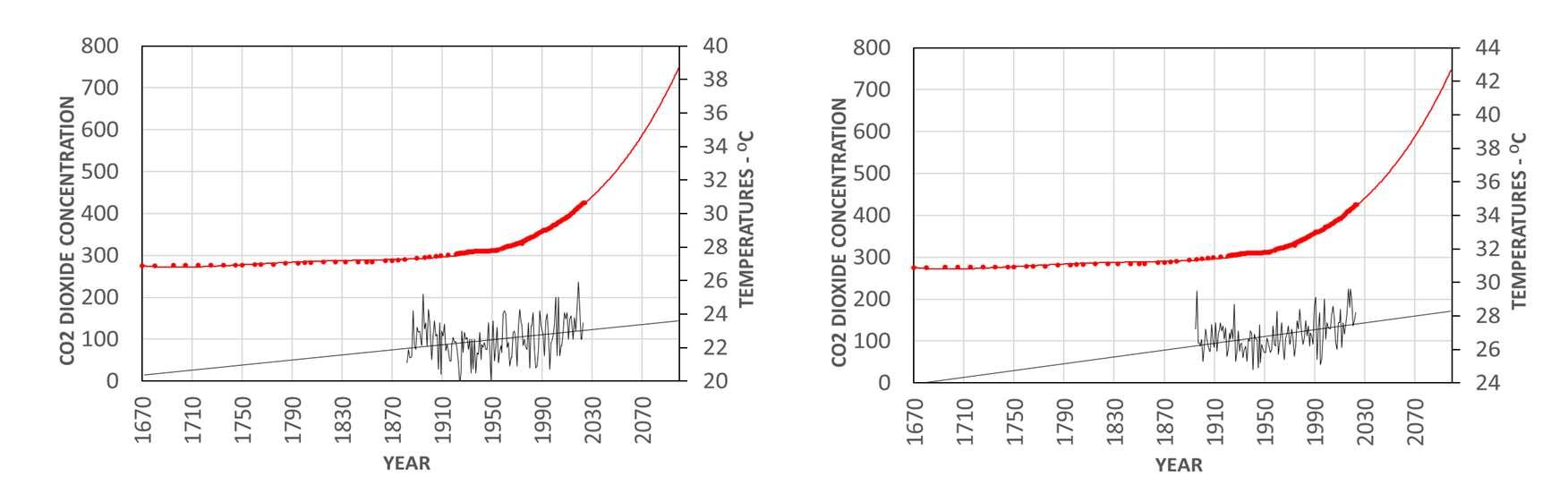
Figure2:Sydney&CentralEnglandTemperaturesversusCO2Concentrationsfortheoverallperiod,1650to2100

https://scienceofclimatechange.org

Notethehugeannualvariabilityintheoriginaltemperaturegraph(Figure1)whichisachallenge toanyanalysisbasedonaveragescalculatedforsmallperiodswithinthefulldaterange.

Figure3:CarbonDioxideConcentrationversusPopulationGrowthinSydneyfortheperiods1740 (CO2)and1788to2023(population)

3.UrbanEffectonTemperature

Using the increasing population of Sydney to represent the increasing population of the world, Figure 3 indicates a degree of correlation between population and the increasing global concentrationofCO2 causedbytheincreasingnumberofpeople,vehiclesandothermachinerythatemit anincreasingvolumeofCO2 overtheyearsinanurbanenvironment.

There is a phenomenon known as the urban heat island(UHI) [11] that, it is claimed, affects temperatures recorded in cities such as Sydney. Considering all the sources of heat that exist in a city compared to the countryside, it is not surprising that the UHI exists. For example, the population of ~5 million people in Sydney generates an average of 100 Watts per person which totals500MW,althoughadmittedly,thisheatisspreadverythinlyoveranareaofapproximately 12,367squarekilometres. Addtothistheheatbeinggeneratedbyallthe(heat-emitting)machinery that exist in a large city and it is not surprising that when combined, these factors have an impactonthetemperaturesbeingrecordedincities.

In the book, “The Urban Physical Environment: Temperature and Urban Heat Islands”, by GordonM.Heisler,AnthonyJ.Brazel[14]andpublishedin2010,iswritten:

“…..The UHI effect is strongest with skies free of clouds and with low wind speeds. In moist temperate climates, the UHI effect causes cities to be slightly warmer in midday than rural areas, whereas in dry climates, irrigation of vegetation in cities may cause slight midday cooling compared to rural areas. In most climates, maximum UHIs occur a few hours after sunset; maximum intensities increase with city size and may commonly reach 10°C, depending on the nature of the rural reference. Since the recognition of London's UHI by Luke Howard in the early 1800s, UHIs of cities around the world have been studied to quantify the intensity of UHIs, to understand the physical processes that cause UHIs, to estimate the impacts of UHIs, to moderate UHI effects, and to separate UHI effects from general warming of Earth caused by accumulation of greenhouse gases in the upper atmosphere…..”

Alsowritten:

“…...Despite considerableresearch, many questions about UHI effects remain unanswered. For example, it is still not clear what portion of the long-term trends of increasing temperatures at standard weather stations is caused by UHI effects and how much is contributed by greenhouse gas effects. Also not well quantified is the effect of increasing tree cover in residential areas on temperatures…..”

Regardless of the above and other related phenomena, this paper only considers the outcome of thecombinedeffectofallthemeteorologicalprocessesintermsofthetemperaturesmeasuredat specificcityandregionalsites.

4.TypesofTemperaturesMeasured

In the case of the Sydney temperature data, two sets are used in this paper corresponding to a compilationofthe highesttemperature recordedineachyearinone set,andthe lowesttemperaturerecordedineachyearintheother. Figure4showsthetwosetsoftemperaturedatacovering theranges,1860to2023forminimumtemperaturesand1895to2023forthemaximumtemperatures for each year along with CO2 concentrations. The graph includes boundary lines parallel totheTrendLinesandenclosingtheextremesofeachofthetemperaturedatasets.

Figure4:CarbonDioxideConcentrationversusHighest&LowestAnnualTemperaturesinSydney fortheperiod1859to2023

AnunexpectedoutcomewhencomparingtheSydneyandCentralEnglandtemperatures,wasthat theirratesofincreaseweresimilardespitethetwolocationsbeinginoppositehemispheresofthe world and separated by over 17,000 kms – the similarity is demonstrated in Figure 2 where the TrendlineforCentralEnglandhasbeencopiedandpastednexttotheTrendlineforSydney. Part ofthedifferencecouldbeduetodifferent“adjustments”madebyeachoftheMetBureaustothe rawtemperaturedata.

5.InterpretationoftheGraphsandResultingPredictions

The graphs allow the levels of temperatures for the next few decades to be predicted with

reasonableaccuracysincetheobservablevariationsoftemperatureinmanyofthechosensitesas measuredfromtheTrendlines,havebeenconsistentforwelloveracentury,evenduringthelater years(1980sandbeyond)whentheconcentrationofCO2 begantoincreaseexponentiallybeyond its previous levels for the earlier period, 1740 to 1940. The consistency of the data is discussed further in Section 7 where a distinct discontinuity at or near the year 1950 in the anomaly data sourcedfromtheAustralianBureauofMeteorologywasdiscussed(highlightedwithTrendlines) in Figure9. Itwasassumedthattheanomalydata was derivedfromthetemperaturedataand as expected,asimilardiscontinuitywasdetectedinthetemperaturedataforthecombinedAustralian citiesaroundaboutthedate,1950(Figure11).

The graphs appearing in this paper show there is little (if any) correlation between the rate of change of the concentration of CO2 and that of the temperatures measured at any of the sites examined. If therewere, withcarbondioxideasthe “driver”,therewould be a noticeable exponentialincreaseintemperatureswhentheconcentrationlevelofCO2 begantoincreaseexponentiallyduringthe1940sandbeyond. Despitethediscontinuitymentionedabove,overall,thetemperatures in Sydney and the other sites were seen to continue to rise at approximately the same linearrateasforthepreviouscenturiesregardlessofchangesintheconcentrationofatmospheric CO2

The extreme temperature boundary lines in Figure 4 indicate that in all the years leading up to 2100, higher annual(ieextreme)temperatures could berecorded at Observatory Hill in Sydney. Temperatures in regions, inland from Sydney, will be different, depending upon their locations; example-theouterregionsof SydneysuchasPenrith(~50kmswest) willalwaysrecordhigher averaged annual temperatures than those recorded at Observatory Hill which was the source of temperature data for Sydney in this paper. Analysis of the available data showed that Penrith maximum annual temperatures were an average of 4 OC warmer than Sydney with a possible extremehightemperatureof6 OCwarmerthanSydney. Sydney,beinglocatednexttotheocean, has the benefit of cool sea-breezes that lower its temperatures, a benefit not shared by inland cities.

6.CO2 ConcentrationsandHealth

It is worth noting that if the concentration of CO2 continues to increase in line with a 4th degree polynomial, the predicted concentration of CO2 by 2240 will be about 2,600 ppm compared to the current concentration of ~420 ppm. This is not alarming for human activity based on the safetyparametersforCO2 concentrationssetbyOSHA,theOccupationalSafetyandHealthAdministration of the USA. They seta permissible exposurelimit(PEL) for CO2 in the workplace at5,000partspermillion(ppm)overan8-hourworkday. However,theyalsowarnedthatexposure to concentrations higher than 5,000 ppm could cause adverse symptoms such as headache, dizziness,increasedheartrate,confusion,andinextremecases,unconsciousness,ordeath.

Based on the above information for CO2 concentrations, today’s humanity should not be concernedaboutthepossibilityofadversehealtheffectsfromeven2,600ppmconcentrationofCO2, aspredictedfor2240,216yearsintothefuture.

However,thefuturelevelsofCO2 concentrationremainuncertainbecauseofthemultiplefactors thataffectitsconcentration.

Currentattempts bygovernments toreduce globalCO2 emissions from coalpoweredpower stations have been hampered by China as well as the reliance of developing countries on coal for electricitygenerationandtheslowgrowthofreliablecapacityfromalternativesources. Thelikely outcome of all these factors is a continuation of the rise in CO2 concentration as shown by the graphs. Disregarding the various mechanisms that could affect the concentration of CO2 in the atmosphereofwhichtherearemany,forsimplicityitwasassumedthattheconcentrationofCO2 in the atmosphere would continue to rise in a manner similar to the rises already experienced duringthepastfewdecades.Althoughtherearecertainlyotherfactorsthatinfluencetheconcen-

tration of CO2, it is not the intention of this paper to investigate those factors or their effects –only to look at the outcome of those factors to date, and to extrapolate from that data into the future

Finally,inconsideringtheincreasingconcentrationofCO2 intheatmosphere,therewasnoother choicebut to acceptthe data published on various websites; in this case, the website [12] which contained an interactive graph from which the CO2 data was extracted and graphed as shownin Figure5.

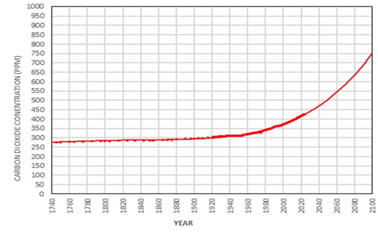
Figure5:Concentrationsofcarbondioxideusingdatafrom1740to2023andextrapolatedtothe year2100.

7.IntegrityoftheTemperatureDataUsed

It has beensaidthat it isvery difficult to acquire actual rawtemperature data. Inthe 1990's one couldseerealrawdatafromanyUSmonitoringstation,butsinceabouttheyear2000,thataccess hasbeenshut off. What isavailable nowisadjusteddata. Thesamecanbesaidfor thetemperaturedataforAustraliancitiesandtownsusedinthispaper,sourcedfromtheAustralianCSIRO Bureau of Meteorology website, and for global cities, sourced from weather bureau websites in theircountries. Justhowthatdatahadbeenadjustedbeforebeingpublishedisunknown–atleast, unknown to this author. Although it is highly likely that the temperatures have indeed been adjusted,thisauthorhadnootherchoicebuttoacceptthemsincetherewerenootherreliablesources oftemperaturedataavailable.

“Adjustments” to temperature records may not always provide results that are consistent with reality as observed in a detailed discussion by experts about the homogenization of temperature records. It is accepted that providing consistent and accurate temperature records from several diversereportingstationsoveralargenumberofyearsisnotaneasytask.

Intheir jointpaper,“Evaluationofthe HomogenizationAdjustmentsAppliedtoEuropeanTemperature Records in the Global Historical Climatology Network Dataset”, the following commentsweremadebytheauthors:

“.......after comparing the different homogenization adjustments applied by the National Oceanic and Atmospheric Administration (NOAA) to their widely used Global Historical Climatology Network (GHCN) monthly temperature dataset, we found a disconcerting inconsistency between the updates to the dataset from day to day......“ and:

“........this remarkable inconsistency in the results from NOAA’s application of the Pairwise

Homogenization Algorithm (PHA) to the GHCN since 2011 is quite surprising since the PHA has performed quite well over the years against various benchmarking tests. However, we note that those earlier assessments of the PHA were generally “one-off” assessments, i.e., they did not evaluate the consistency of the breakpoints and adjustments applied with repeated runs of the algorithm. Therefore this inconsistency of the PHA adjustments between consecutive runs would have been inadvertently overlooked by those earlier tests....“

and:

“...we believe these findings should be used as motivation for improving our approaches to homogenizing the available temperature records. Meanwhile, the results raise serious concerns over the reliability of the homogenized versions of the GHCN dataset, and more broadly over the PHA techniques, which do not appear to have been appreciated until now.....“

However, the prediction of temperature rises made in this paper should hold true providing (a) the AustralianMet Bureau (andtheotherbureaus) continue to “adjust”their temperaturedatain thesamemannertheyhaveusedduringthepastfewdecades,and(b)whateverbiasestheymight haveembeddedintheir“adjustment”processesdonothaveanincreasinglyunrealimpactonthe consistency of temperatures being reported. The impact of such “biases”, if they have been incorrectlyconstructed,maynotbeevidentfortenortwentyyearsbywhichtimeitwillbetoolate to halt the expenditure of trillions of dollars to combat what will have turned out to be a nonexistent problem. Should that happen, the temperatures being reported will be higher than the raw temperaturesbeingrecordedalthoughthis discrepancymaynotbe noticedbythepublic for afewmoreyears.

This author has made intensive use of temperature data available from the Australian Bureau of Meteorology,anexampleofwhichisFigure6.

Figure6:AustralianSurfaceTemperatureAnomalies*onlyavailableingraphicalform–digitalizedinFigure7toallowlatercomparisonwithothertemperaturedataalreadyindigitalformat.

*Atemperatureanomalyreferstoadeviationfromthelong-termaveragetemperatureforaspecificlocationorregionoverasetperiodoftime.It'sameasureusedinclimatesciencetoassess howmuchwarmerorcoolerthetemperatureiscomparedtotheexpectednormforthattimeand place.Anomaliescanbepositive(warmerthanaverage),negative(coolerthanaverage),ornear zero(closetothelong-termaverage).

https://scienceofclimatechange.org

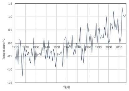
Figure7:ResultofdigitalizingtheAustraliandata(showninFigure6).

Toallowtheanomaliesdatatobecomparedgraphicallywithtemperature,itwasfurthermodified by adding 33 OC to each of the data points. This process did not alter the important factor discussedinthispaper–the rate of change oftemperatures.

Later,duringtheanalysis,itwasnoticedthattheTrendlinefortheBureau’sAnomaliesdatahad a similar rate of change as that for the temperatures averaged over six of the seven Australian cities (temperature data for Perth did not cover a sufficient range of dates to be included). Furthermore,byaddingaspecific28.9 OCtoeachoftheanomalytemperaturepointsshowninFigure 7, the trend lines for the anomalies and temperatures graph almost coincided as from 1950, as showninFigure10.

Figure8:Anomaliesplus28.29OC

The first trend line (brown) for the anomalies data in Figure 9 for the period ending in 1950 indicatedamoderatelyconsistent,butverysmallriseintemperatureof0.001 OCperyear.

ThesecondTrendline(blue)fortheAnomaliesdatafrom1950to2017showsamuchlargerand consistentriseof0.019 OCperyear.

Thecauseofsuchadiscontinuityoccurringovertwoyearsorless,cannotbeexplainedeasilyas being the influence of either CO2 concentrations or natural processes since changes caused by CosmicandGlobalinfluencesoccurovermuchlongerperiods,sothediscontinuitywasassumed tobecausedbyachangeinthemethodusedbytheBureauto“adjust”theirtemperaturerecords.

Figure9:ThefirstTrendline(brown)isthatforanomaliesdatafromAustralianBureauofMeteorology,fortheperiod,1910to1950.ThesecondTrendline(blue)isanomaliesdatafortheperiod 1950to2023.

Trend lines for Anomalies (red) and Averaged Australian Cities data (black) are compared in Figure 10 and show close correlation between the two variables for the period 1950 to 2022 as seenfromthesetof(almost)overlappingblackandredTrendlines.

Figure10:Acomparison-combinedAustralianCitiesAveragedHigh-Temperatures(black)versus Anomalies(red)-1950to2017.

The discontinuity at the end of the period 1949-1950 shown in the Anomalies graph (Figure 7) alsoappearsinthecombinedAustraliancitiestemperaturegraph(Figure11). Thisisnotsurprisingsincethedataforbothvariablesisfromthesamesource,theAustralianBureauofMeteorology,andmostlikelysubjecttothesame“adjustment”,albeit,asfrom1950.

Itwasnotthepurposeofthispapertoinvestigatethereasonsbehindtheapparenterratictemperature measurements prior to 1950 or the complex method of “adjustments” applied to the post 1950raw dataandsofor simplicity, hasfocusedonmeasuringthetemperature trendspost 1950 forthethreecategoriesexamined:namely,(a)allAustraliancities(averagedhightemperatures), (b) a selection of Australian towns (averaged high temperatures), and (c) a selection of Global citiesandregions(averagedtemperatures).

MeasurementsoftheratesofchangeoftemperaturesfromthosestudiesaresummarisedinTable 1.

Ian McNaughton: Temperature Measurements Versus CO2 Concentrations & Population Growth

Figure11:AveragedPreandpost1950AustralianCitytemperatures.

Some cities and towns were omitted from the calculations due to insufficient temperature data beingavailable. Theywere:

AustralianCities: Perth

Australiantowns: Albany,Oodnadata,Cloncurry,BurrinjuckDam

GlobalCities/Regions:Bangkok

Table1:Predictionsfortheyear2050comparedto2024levels(calculatedfrompost-1950temperaturedata).

Thepredictionsfortheyear2050(comparedto2024levels)are:

 rateoftemperaturechangeaveragedoverallcitiesandtownsstudied: 0.018 OC/year,

 riseintemperatureaveragedoverallcitiesandtownsstudied: 0.47 OC,

 maximumtemperatureatObservatoryHill,Sydney: 30.0 OC,

 extremetemperaturesthatmightoccuratObservatoryHill,Sydney: 32.0 OC,

 extremetemperaturesthatmightoccuratPenrith(NSW): 38.0 OC,

 concentrationofCO2 intheatmosphere: 500ppm.

Shouldtemperaturesasmeasuredbythe AustralianBureauofMeteorology andotherglobal climate bureaus, continue to be adjusted as they have since 1950, Table 1 shows that the expected rise in temperature averaged over allthecities andtowns examined, will be 1.37 OCby the year 2100.

AnotherobservationoftheGlobalcitytemperatureswastheabsenceofanydiscontinuityduring the period 1949-1950. Figure 12 shows the Trend lines generated for (a) a subset (black) of Global City temperatures covering the period 1910 to 1949, (b) a second subset (green) 1950 to 2023andathirdfullset(brown-hidden)1910to2023.

Figure12:GlobalCityTemperatures-threeSets:1906-1950,1950-2100&1906-2100.

InFigure12,theaverageGlobalCitytemperaturesat2100calculatedfromthelinearTrendLines forpreandpost1950data,differbyonly~0.7 OCthussupportingtheassertionthatifanyadjustmentshadbeenmadetotheGlobalCitiesdata,thentheywereappliedtothedatasetscorrespondingtothefulldate-range.

Neither of these two sets of temperatures show any visible correlation with the exponentially increasingconcentrationsofCO2.

8.InterglacialCyclesoverthePast450,000Years

This paper supports the assertion that it is local, global, and cosmic forces and not atmospheric CO2 concentrationsthataredrivingthemassivechangesinclimateexperiencedbytheearthduring the past 400,000+ years as shown by the five major cycles in Figure 13 [13]. It therefore dependsuponwhereweareintheglacialcyclesastowhetherthecurrentincreasesintemperature willcontinue.

Figure13:Temperaturesobtainedfromglacialrecordsforaperiodof450,000years.

Although the overall rates of temperature changes either up or down during the major glacial cycles are small, within the sub-cycles of major glacial changes, temperature changes can be in eitherdirectionandatmuchhigherrate,anditisassumedthattheearthisinsuchasub-cycle. The range of years important in this paper, 2023 to 2100, is within a glacial sub-cycle and very small comparedto Interglacial time periods. Figure 13 provides anindication of just how small thattimeframeis;nevertheless,itisthetimespanthatconcernshumanity.

Measurementsfromglacialsub-cyclesshowthattherateofchangeoftemperaturecanvaryfrom 0.014to0.025 OCperyear. TheaverageofmeasurementsfromcurrenttemperaturerecordssummarisedinTable1(0.018 OCperyear)liewithinthatrange.

Ifthecurrentrateofchangeofmeasuredtemperaturescontinues,thetemperaturesthatwouldbe recorded at Observatory Hill, 10,000 years from now, might be considered by some as being moderatelyuncomfortablebutstillbearable. However,thispaperconcludesthereislittlehumanitycandotoavoidtheserises,sincetheywould not becausedbythe higherCO2 concentrations intheatmosphereexpectedthen.

Unlesstheworlddestroysitselfinthemeantime,withinthose10,000years,advancesintechnology might finallyfinda solution to addressthe problem – if there is a problem. The world may also be at a different stage of the inter-glacial cycle when the global temperature might even be reducing,andnosuchsolutionwouldberequired.

9.CarbonCycle

When the author was attending secondary school, the carbon cycle [15] was part of the curriculum. In those days, the concept was simple with no concerns about the concentration of carbon dioxide in the atmosphere. The Carbon Cycle in Figure 14 shows carbon dioxide being both absorbedandreleasedbytrees,vegetation,lakes,seas,oceansandanimals. Duringthehundreds ofmillionsof yearsof the earth’shistorywhenplantand animallifeflourished,aportionofthat carbondioxidewasbeinglockedupindepositsofcoal,oil,gasandsomeminerals.

Figure14:TheCarbonCycle.

The carbon cycle was strongly impacted by the industrial revolutionand beyondthroughtheincreasinguseofmachinerythatutilisedgas,coalandoiltoprovide energy.Burningthat coal,oil or gas returned CO2 back to the atmosphere. Suddenly, carbon dioxide that hadbeen stored for hundredsofmillionsofyearswasbeingreleasedbackintotheatmosphereatamuchfasterrate–aratethathasbeenincreasingexponentiallysincethe1940sto1950s.

It was exceedingly easy for alarmists to link increasing global temperatures with the increasing concentrationsofCO2 intheatmosphereand forthoselookingforacause,thatconceptwaslike agiftfromheaven.

Forgovernments,itprovidedreasonstoappeartobecompetent,knowledgeableandcaring–and to spendtrillions of dollarssupportedbythose who declaredthat“the science isin”thusstifling furtherdebate.

Fortheprivatesector,theopportunitiesformassiveprofitsweretootemptingtoignore.

Foractivistslookingforacause,the(apparent)CO2 issuesatisfiedalltheirdesires.

Thispapershowsthatthescienceis“notin”andconcludesthatCO2 isnotapollutant! Quitethe opposite-CO2 isanessentialpartoflife.

10.SevenAustralianCities

Since the Australian government is very concerned about Australia’s contribution to what they regardasthecauseofglobalwarming,CO2,itwasthoughtappropriatetofinishthepaperwitha presentation of the temperature variations over the past centuries for each Australian city and comparethemwiththeincreasingconcentrationsofCO2.

The graphs in Sections 11, 12 and 13 show the variation of the highest temperature (or in some cases,theaveragetemperature)recordedforeachofthecities,townsandregionsforeachyear.

AlthoughbothglobaltemperaturesandCO2 concentrationsareincreasing,thereisnovisibleevidenceinthegraphsforthe19cities,townsorregionsincludedinthisstudy,thatcorrelatestemperatureincreaseswiththe exponentially increasingCO2 concentrations.

Itisusefultonotethatthedatausedforthispaperisfreelyavailableontheinternetforanyoneto use,andtheURLsusedtosourcethatdataareprovidedintheReferenceSectionshouldanindependentcheckbeconsideredasnecessary.

Realistically,theman-in-the-streetis not interestedintemperatureanomalies–they areonlyinterested in and affected by the actual temperature they are experiencing – surface temperatures thatarerecordedbytheirlocalmeteorologicalstations. Thosetemperaturesareusedinthispaper and shown in the graphs although there are strong signs they may no longer be “raw” measurementsandthat“adjustments”tothemhaveprobablybeenmadebytheAustralianBureauofMeteorology.

Ideally, unadulterated raw temperatures would have been far preferable for this paper, but they werenotavailable.

ThegraphsforAustraliancitytemperaturesdiscussedinthispapershowthehighesttemperatures recordedeachyear foreachcity.AfewAustralianmediaoutletsdelight indescribingsome current weather events/temperatures as “extreme”, and that such weather events have never been experiencedbefore.

TheAustralianBureauofMeteorologyprovidessupportfortheseclaimsbythemediaoutletsby statingonitswebsite:

“……Australia’s weather and climate continues to change in response to a warming global climate..........with most warming since 1950. This warming has seen an increase in the frequency of extreme heat events.....eight of Australia’s top ten warmest years on record have occurred since 2005........increases in temperatures are observed across Australia in all seasons with both day and night temperatures showing warming. The shift to a warmer climate in Australia is accompanied by more extreme daily events….“.

Figure 4, which shows the rise in high temperature measured in Sydney from 1880 to 2023, includesaboundaryforthemostextremetemperatureexperiencedduringthatperiod. Astheyears

Ian McNaughton: Temperature Measurements Versus CO2 Concentrations & Population Growth

pass by, the boundary of the most extreme temperature also rises, and so it is logical that future extremetemperatureswillbethehighesteverrecorded.

Theaverage annualincreasein temperaturefor the sevenAustraliancitiesandtownswascalculated to be 0.017 OC per year so the increase in temperature by the year 2050 (26 years into the future)wascalculatedtobe0.44 OC,or1.29 OCbytheyear2100aslistedinTable1.

Some may still argue that drawing a conclusion from the analysis of data from only five global cities, seven Australian cities and some Australian towns is not sufficiently rigorous to be acceptedbythescientificcommunity. Beforeadvancingthatargument,itwouldbeappropriatefor them to obtain and graph temperature data for any city/cities inthe world they might choose. It isunlikelytheirconclusionswoulddifferfromtheconclusioninthispaper.

For consistency, the following graphs were constructedwith the full data sets available for each cityandtown. Some of those data setssuchastheoneforBangkokcover onlyasmall rangeof dates.

NoneofthegraphsshowanyvisiblecorrelationbetweentherapidlyrisingconcentrationsofCO2 andtherisesintemperature.Theydo,however,showrisingtemperaturesinalmostalllocations, aswasexpected.

11.TemperaturesversusCO2 Concentrations–SevenAustralianCities

https://scienceofclimatechange.org

HOBART SYDNEY

MELBOURNE

BRISBANE

PERTH

ADELAIDE

Ian McNaughton: Temperature Measurements Versus CO2 Concentrations & Population Growth

DARWIN SIXAUSTRALIANCITIES

12.TemperaturesversusCO2 Concentrations–SevenAustralianTowns

CAIRNS KALGOORLIE

ALICESPRINGS

Science of Climate Change

https://scienceofclimatechange.org

BURRINJUCKDAM

THREEAUSTRALIANTOWNS

13.TemperaturesversusCO2 Concentrations-FiveWorldCities/Regions

CENTRALENGLAND

Ian McNaughton: Temperature Measurements Versus CO2 Concentrations & Population Growth Science of

BOSTONMASSACHUSETTS

https://scienceofclimatechange.org

BANGKOK FOURGLOBALCITIES

ALABAMA

SACRAMENTO

Ian McNaughton: Temperature Measurements Versus CO2 Concentrations & Population Growth

14.Conclusion

TherelationshipbetweentheexponentiallyincreasingglobalconcentrationsofCO2 andincreasing global temperatures for all the sites studied has been shown to be tenuous at least, and most likely,non-existent.

The findings in this paper strongly suggest that increases in the concentrations of global atmospheric CO2,regardlessofits sources,shouldno longerbeof concernto humanity,bothnowand inthefuture,andthatthetrillionsofdollarsbeingwastedonprojectstoreduceoreliminateCO2 emissions,beimmediatelyredirectedtoessentialworkthatwillbenefithumanity.

Increasesintheconcentrationof CO2 in the atmospherearenot aproblem– itisquite theopposite! It can only improve the quality and abundance of plant growth that has occurred during someofthepastmillenniawithoutharmingtheworld’sinhabitants.

WhethertheconcentrationofCO2 increases,decreasesorremainssteadyshouldbeofnoconcern to humanity –therisein globaltemperature willcontinue atitscurrentrateof0.018 OCperyear fortheforeseeablefuture,independentofCO2 concentrations.

There is, however, a clear (and expected) correlation between the increasing concentrations of CO2 andtheincreasingpopulationoftheworld,asrepresentedbythepopulationgrowthinSydney. TheproblemhereisnottheCO2 -itistheabilityofgovernmentstosustainhigherlevelsof populationsintermsoffood,transportandaccommodation.

Funding: JohnMcRoberts.

Chief-Editor:H.Harde;Reviewers:anonymous.

Acknowledgements

The author would like to thank Prof Gabriël Moens, John McRobert and Ted Mouritz for their assistanceandadvice.

References

1. TemperatureDataAdjustments:https://www.bom.gov.au/akamai/https-redirect.html, https://www.mdpi.com/2073-4433/13/2/285

2. ClimateChangeScepticism:https://www.ncbi.nlm.nih.gov/pmc/articles/PMC3002211/

Science of Climate Change

https://scienceofclimatechange.org

3. AustralianCity&TownTemps:https://reg.bom.gov.au/climate/data/stations/

4. CentralEnglandAverageTemps:https://theconversation.com/june-2023-was-the-hottest-inengland-since-1846-heres-why-it-was-so-unusual-208692

5. AlabamaAverageTemperatures:https://www.ncei.noaa.gov/access/monitoring/climate-ata-glance/county/time-series

6. BangkokTemperatures:https://en.tutiempo.net/climate/ws-484550.html

7. BostonMassachusetts:https://www.currentresults.com/YearlyWeather/USA/MA/Boston/extreme-annual-boston-high-temperature.php

8. Sacramento:https://www.currentresults.com/YearlyWeather/USA/CA/Sacramento/extreme-annual-sacramento-high-temperature.php

9. Trend(BestFit)Lines:https://help.tableau.com/current/pro/desktop/en-us/trendlines_add.htm

10. SydneyPopulation:https://en.wikipedia.org/wiki/Demographics_of_Sydney

11. UrbanHeatIsland:https://acsess.onlinelibrary.wiley.com/doi/abs/10.2134/agronmonogr55.c2

12. GlobalCO2 Concentrations:https://www.co2levels.org/#sources

13. GlacialandInterglacialperiods:https://energyeducation.ca/encyclopedia/Glacialandinterglacialperiods;https://skepticalscience.com/print.php?r=337

14. G.M.Heisler,A.J.Brazel,2010: The Urban Physical Environment: Temperature and Urban Heat Islands,https://acsess.onlinelibrary.wiley.com/authored-by/Heisler/Gordon+M.

15. TheCarbonCycle:https://scied.ucar.edu/image/carbon-cycle-diagram-nasa

https://scienceofclimatechange.org