EXECUTIVE SUMMARY
The Cox Creek site is a dredged material containment facility (DMCF) located in the Baltimore Harbor. The site is an upland disposal site anchored to land, with a diked containment area projecting into the Harbor. The Cox Creek DMCF was first operational during the 1960s through 1984. Between 2002 and 2006, the Cox Creek DMCF site underwent modifications in order to accept additional dredged material from the Baltimore Harbor. In the past, Baltimore Harbor material was placed in the Hart-Miller Island Dredge Material Containment Facility (HMI DMCF). However, the HMI DMCF stopped accepting dredged material at the end of 2009. As a result, the Cox Creek DMCF has recently become more active in receiving material dredged from the Baltimore Harbor; first large inflow was received in 2012 To date, the Cox Creek DMCF has received approximately 2 million cubic yards of dredged material.
In order to assess any effects of the reactivation and operations of the Cox Creek DMCF, ten monitoring sites were established around the exterior of the facility: nine (9) monitoring sites adjacent to the area and one site designated as a reference site. Sediment samples were collected annually between 2006 and 2010. No exterior sampling was done in 2011 and 2012 due to little or no discharge from the facility. Exterior sampling resumed in 2013, representing the sixth year of monitoring during active operations and continued for a seventh year in 2014. Results of the 2014 monitoring are presented in this report.
Maryland Environmental Service (MES) collected the samples and the Maryland Geological Survey (MGS) was responsible for textural and chemical analyses of the samples and interpretation of the results. Samples consisted of undisturbed sediments collected at the sediment-water interface. The sediments were analyzed for textural properties and 51 elements including total nitrogen (N), carbon (C), phosphorus (P), sulfur (S), cadmium (Cd), chromium (Cr), copper (Cu), iron (Fe), manganese (Mn), nickel (Ni), lead (Pb) and zinc (Zn).
Data from samples collected on October 21, 2014 are presented in this report. Placed in a broader context with the results of ongoing monitoring (2006-2014), the data show:
1. Sediments around the Cox Creek DMCF are generally fine grained and exhibit a gradient of higher sand content close to the dike, diminishing outwards toward the channel and downstream. This distribution pattern has been reproduced during all monitoring years.
2. As derived from the total N and total P content of the sediment, the sediments adjoining the Cox Creek DMCF study area receive the majority of their organic matter from terrigenous sources rather than planktonic sources.
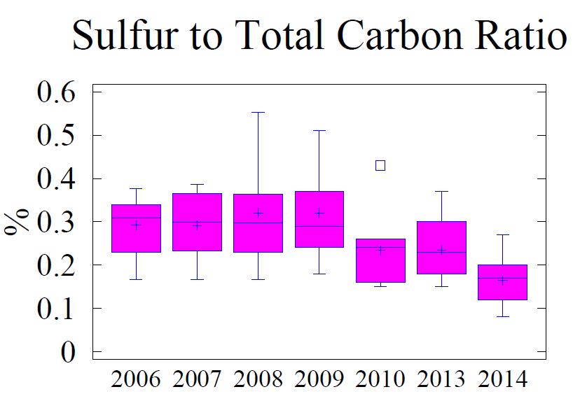
3. The sulfur to carbon ratio is lower than that measured further into the Harbor, indicating that the area is slightly more disturbed or has a higher sedimentation rate than further into the Harbor.
4. Certain target metals, including Cd, Mn, and Ni, remain within background levels found in the northern Chesapeake Bay. The remaining target metals, including Cr, Cu, Fe, Pb and Zn, are elevated above background levels. Forty percent of the sites are enriched in Zn. Ninety to 100 percent of the sites were significantly enriched with Cr, Cu, Fe, Pb.
5. Target metals in the study area follow the general patterns seen in the 1994 - 1997 Baltimore Harbor Spatial Mapping studies (BHSM, Baker et al, 1997, Mason et al 2004). The sediments exterior to the Cox Creek DMCF appear enriched in Fe and Pb, and to a lesser extent, in Cr, Cu and Zn relative to some, but not all, areas of Baltimore Harbor.
6. Physically and chemically, the reference site is not representative of sediments
1
immediately exterior to the DMCF. Large variations in sediment texture have occurred at the reference site; for example the % sand has ranged more than 50% (from >60% in 2007 to < 10% in 2008) and the clay-to-mud ratio (CMR) ranged more than 20%. The reference site helps provide spatial coverage which suggest additional external source of regional metals, but may not be a good gauge to measure changes due to operation of the DMCF. Therefore changes due to operation of the DMCF are best evaluated through monitoring any changes to the exterior sediments over time.
7. The spatial pattern of the metals concentrations, expressed as sigma level contours, for all elevated metals (Cr, Cu, Pb and Zn) depicts the entire area of sediments adjoining the Cox Creek DCMF as significantly enriched in these metals. The local sigma maximum was observed at sampling station #8 during the 2014 event, located to the southeast of the DMCF, consistent with most preceding monitoring years. Over time (2006-2014), there has been no observable increase in size of the area with metals enrichment nor has there been any upward trend in the magnitude of metals enrichment (as expressed in sigma levels) in the sediments adjacent to the facility. We interpret the stability of spatial pattern, size and magnitude as indicative of no outward effects from the Cox Creek DMCF operations to the exterior sedimentary environment.
2
INTRODUCTION
The Cox Creek DMCF is located in the Baltimore Harbor. The site is an upland disposal site anchored on land, with a diked containment area projecting into the Harbor The site is designed to accept dredged material from the Baltimore Harbor, and eliminate overboard disposal of dredged sediment. The site is similar in design to the HMI DMCF. Based on the monitoring history of HMI DMCF, if the Cox Creek containment areas are maintained in a similar manner no adverse environmental effects are anticipated. However, it is crucial to ensure that the placement of dredged material does not have any unanticipated adverse effects on the environment. A scheduled routine monitoring program has been put in place to track any changes to the sedimentary environment immediately exterior from the DMCF The Cox Creek DMCF began accepting dredged material in 2005. Annual exterior sampling began in 2006 and continued annually until 2010 There was a two year hiatus in the exterior monitoring due to little or no inflow into the facility or discharge from the facility. The first large Harbor maintenance inflow project was received in 2012, therefore exterior sampling resumed in 2013, representing the sixth year of monitoring during active operations, and continued for a seventh year in 2014. Results of the 2014 monitoring are presented in this report.
Objectives
The objectives of the sediment quality monitoring project are:
1. To measure physical parameters and the concentration of metals and other chemicals in the sediment that could be indicators of accompanying effects to the benthic infauna and potential bioaccumulation through the food chain;
2. To document any changes in the exterior physical sedimentary environment due to the construction at and operation of the site; these changes are to be placed into a regional context so that the changes can be properly interpreted, and;
3. To provide a framework of the physical/geochemical sedimentary environment for the benthic infaunal studies.
BACKGROUND
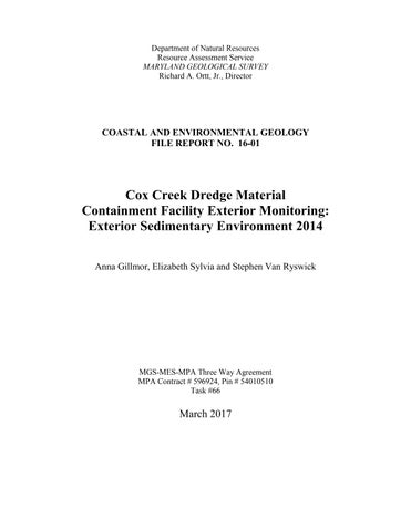
The Cox Creek DMCF is located approximately one mile south of the Francis Scott Key Bridge, on the western shore of the Patapsco River in the upper Chesapeake Bay (Figure 1). The facility is one of three DMCFs in the Baltimore Harbor vicinity; the HMI DMCF and Masonville DMCF are the other two. The U.S. Army Corps of Engineers Baltimore District originally constructed the Cox Creek DMCF in the mid-1960s. This site was used periodically from the mid-1960s through 1984. The Maryland Port Administration (MPA) purchased half of the site in 1993 and the other half in 1997. Between 2002 and 2006, the Cox Creek DMCF underwent modifications in order to accept dredged material from the Baltimore Harbor. Until recently, dredged material from the Baltimore Harbor was placed in the HMI DMCF. However, the HMI DMCF was closed to new dredged material at the end of 2009. Although the Cox Creek DMCF has been accepting dredged material since 2005, the facility has become more active in receiving material dredged from the Baltimore Harbor since 2012
The Cox Creek DMCF consists of two cells (Figure 1), and is designed to accept an average
3
of 500,000 cubic-yards (cy) per year of dredged material (Kotulak and Headland, 2007) The Cox Creek DMCF covers 133 acres with 102 acres usable for dredged material placement. This site is roughly 10% of the size of the HMI DMCF or the Paul S. Sarbanes Environmental Restoration Project at Poplar Island (PIERP) At the current dike elevation of +36 feet above mean lower low water (MLLW), the Cox Creek DMCF will hold approximately six million cubic-yards of material dredged from various sites within the Baltimore Harbor including the Federal shipping channels. The original designed site life was 12 years based on a projected inflow of 500,000 cy per year of dredged material from maintenance and new work dredging in the Harbor. Currently the site is projected to be filled by 2020. An expansion of Cox Creek has been approved and dikes will be raised to +80 feet above MMLW and an additional 96 acres of upland area will be available for placement; extending the life of the DMCF Innovative reuse of the dredged material is also continuously researched and could possibly reduce the annual placement volume of dredged material to the facility and thus further extend the operating life of this DMCF.
OPERATIONS
The facility operational goals are to:
1. Optimize site capacity for dredged material through the use of crust management techniques and site modifications;
2. Effectively dewater and dry dredged materials while maintaining water quality standards regulated under a discharge permit from Maryland Department of the Environment (MDE), and;
3. Enhance the Swan Creek Watershed by monitoring and maintaining the created tidal marsh environment adjacent to the DMCF and the associated Forest Conservation Easement
The Cox Creek DMCF began accepting dredged material from the Baltimore Harbor in 2005. Dredged material is placed into the DMCF utilizing hydraulic or mechanical unloading. As of September 26, 2014, over two million cubic yards of dredged material has been placed into the facility, the bulk of which is in the South Cell (Table 1) Normally, inflow/placement is planned for the period between October and April; crust management activities are planned for May through September. However, inflow periods can occur anytime. Discharge occurs mainly during inflow and much lower volumes of discharge occur during crust management. A discharge permit from the MDE sets requirements for water quality, monitoring and reporting.
During periods of discharge, a lime doser may be used to treat water with low pH. When in operation, the inflow and outflow of the doser system is monitored for pH, as well as for Cu and Zn concentrations. Discharges from the facility are monitored daily during discharge, and activities are discontinued if water quality criteria limits do not meet the requirements of the facility discharge permit or if water levels are too low to allow discharge.
4
5
Figure 1: Sampling locations for samples collected in the previous five years and the current study. The upper left is a satellite photo showing the Baltimore Harbor region with Cox Creek blocked out and labeled. An aerial close-up of the Cox Creek DMCF is shown to the right. The aerial photograph was taken September 17, 2013 (NAIP). The lower left figure shows the sampling locations; the Brewerton Shipping Channel marked for reference. The lower right is the site plan; black arrows show approximate locations of the spillways.
Table 1. Cumulative inflow report for the Cox Creek DMCF. Total cubic yardage as of September 26, 2014.
6
Project Name Cubic yards Start Date Finish Date Inflow Point Cell Location Annapolis Channel Harbor Dredging Project 21,257 12/16/2005 1/16/2006 20+00 North Cell Maintenance Dredging at U.S. Coast Guard Station, Annapolis 34,390 9/27/2006 1/17/2007 33+00 North Cell LaFarge @ Curtis Bay MD 9,725 10/2/2007 10/19/2007 38+00 North Cell Rukert Terminals 279,548 10/26/2007 9/26/2014 38+00 North Cell Masonville Cofferdam 6,288 2/4/2008 3/3/2008 38+00 North Cell Masonville Inflow ( 48" Watermain Relocation) 47,968 2/4/2008 8/6/2009 38+00 North Cell Masonville Cell 1 & 1A 1,950 6/30/2008 7/9/2008 38+00 North Cell Pennington Avenue 20 1/28/2009 1/28/2009 38+00 North Cell USCG Yard (Baltimore) 72.16 5/18/2009 5/18/2009 20+00 North Cell Seagirt Berth 4 312,600 5/11/2010 12/15/2011 05+00, 50+00 & 85+00 North & South Cells CSX Bayside Piers 73,200 8/12/2010 2/17/2012 05+00 & 85+00 North & South Cells Constellation Energy/Brandon Shores 15,960 10/13/2010 12/2/2010 05+00 & 85+00 North & South Cells Masonville Outfall 1,900 1/8/2011 1/13/2011 05+00 North Cell Amport 22,550 3/10/2011 5/13/2011 05+00, 50+00 & 85+00 North & South Cells North Locus Point Pier #5 400 4/6/2011 4/6/2011 85+00 South Cell Canton Pier 10 & 11 11,000 5/13/2011 6/8/2011 20+00 North Cell Tydings Memorial Bridge 8,200 8/18/2011 9/7/2013 18+00, 20+00, 40+00 & 50+00 North & South Cells Brandon Shores Constellation Energy 9,590 10/10/2011 10/31/2011 20+00 North Cell General Ship Repair 7,300 2/6/2012 2/29/2012 20+00, 50+00 & 85+00 North & South Cells Jones Fall 92,283 2/28/2012 6/20/2012 50+00 & 85+00 South Cell Pier #5 400 6/1/2012 6/1/2012 85+00 South Cell Fort McHenry 8,125 5/29/2012 6/12/2012 50+00 & 85+00 South Cell Hatem Memorial Bridge 13,075 7/31/2012 7/31/2014 40+00, 45+00 & 50+00 North & South Cells Brewerton Angle 432,656 10/4/2012 10/14/2012 70+00 South Cell USCG Yard (Baltimore) Site #9 5,150 12/13/2012 1/22/2013 40+00 North Cell Fishing Creek 26,955 9/5/2013 11/22/2013 45+00 South Cell Still Pond 15,970 12/16/2013 2/27/2014 24+00 North Cell Harbor Maintenance Dredging thru 2014 598,563 3/10/2014 5/12/2014 70+00 South Cell Total 2,057,095
PREVIOUS STUDIES
Baltimore and the surrounding area in the main-stem of the Chesapeake Bay have been the subject of studies since the early 1970s. However, the most pertinent studies to this project are the on-going monitoring efforts around HMI DMCF (see Sylvia, et al , 2014 and Wells et al , 2015) and the Spatial Mapping of Sedimentary Contaminants in the Baltimore Harbor (Baker et al., 1997, Mason et al 1999, Mason et al 2004.). The 1994-1997 Spatial Mapping studies were the most thorough and comprehensive study of the parameters of interest conducted in the Harbor to date. The studies consisted of physical characteristics, metals and organic compound concentrations which were plotted spatially, as well as comparisons to toxicological screening values. Samples included surficial sediments collected from 80 locations. The main Spatial Mapping study was carried out in 1996 (Baker et al 1997), along with others conducted during the period of 19941997, as cooperative studies with the University of Maryland and MGS, funded by MDE. Although there were only a few samples that fell within the study areas for this report, the Spatial Mapping study provides a broader context for the sites of interest.
The HMI DMCF is a diked containment area in the main stem of the Chesapeake Bay north of the mouth of the Baltimore Harbor. It has been monitored continuously from 1981, just prior to its construction, to the present. The HMI DMCF is similar in construction and operation to the Cox Creek DMCF and the Masonville DMCF. Therefore, if the HMI facilities’ operations impact the exterior sedimentary environment, decisions based on the HMI DMCF model should be directly applicable. Additionally, the HMI DMCF is in the same geochemical regime as the Baltimore Harbor (Hill, 1984; 1988) and the baseline levels determined at the HMI DMCF provide relevant context. The HMI DMCF baseline was used in evaluating the metals data in the Spatial Mapping study.
The results of the HMI and Baltimore Harbor studies will be referred to in the following discussion and were used in the first year monitoring study at the Cox Creek DMCF (Hill, 2007). The results of the previous years’ studies (Hill, 2007, 2008; Hill et al., 2009; Wells and VanRyswick, 2011; Wells et al, 2012; Wells et al, 2015) showed the following:
1. Sediments around the Cox Creek DMCF are generally fine grained and exhibit a gradient of higher sand content close to the dike, diminishing outwards toward the channel and downstream. This distribution pattern has been reproduced during all monitoring years.
2. As derived from the total nitrogen (N) and total phosphorus (P) content of the sediment, the sediments adjoining the Cox Creek DMCF study area receive the majority of their organic matter from terrigenous sources as opposed to planktonic sources.
3. The sulfur (S) to carbon (C) ratio is lower than that measured further into the Harbor indicating that the area is slightly more disturbed or has a higher sedimentation rate than further into the Harbor. This often interpreted as an increase in sedimentation rate, where the rate of biogenic sulfide formation is outpaced by the increased rate of C burial.
4. Certain target metals, including cadmium (Cd), manganese (Mn), and nickel (Ni), remain within background levels found in the northern Chesapeake Bay. The remaining target metals, including chromium (Cr), copper (Cu), iron (Fe), lead (Pb) and zinc (Zn), are elevated above background levels. Forty percent of the sites are enriched in Zn. Ninety to 100 percent of the sites were significantly enriched with Cr, Cu, Fe, Pb.
5. Target metals in the study area follow the general patterns seen in the 1994 – 1997 Baltimore Harbor studies (Baker et al, 1997, Mason et al 2004). The sediments exterior to the Cox Creek DMCF appear enriched in Fe and Pb, and to a lesser extent, in Cr, Cu and Zn
7
relative to some, but not all, areas of Baltimore Harbor.
6. Physically and chemically, the reference site is not representative of sediments immediately exterior to the DMCF. Large variations in sediment texture have occurred at the reference site; for example the % sand has ranged more than 50% (from >60% in 2007 to < 10% in 2008) and the clay-to-mud ratio (CMR) ranged more than 20%. The reference site helps provide spatial coverage which suggest additional external source of regional metals, but may not be a good gauge to measure changes due to operation of the DMCF. Therefore changes due to operation of the DMCF are best evaluated through monitoring any changes to the exterior sediments over time.
METHODOLOGY Field
MES collected the sediment samples and MGS conducted the textural and chemical analyses on the samples and provided interpretation of the results. The samples were collected on October 21, 2014. Samples consisted of undisturbed sediments collected at the sediment-water interface using a Ponar grab sampler. From each of these samples, two sub-samples were taken and packaged in Whirl-pak plastic bags. One sub-sample was designated for textural analysis; the other for metals and total C, N, S and P analysis. After collection, the samples were stored at 4° C until analysis and were analyzed less than 6 months after delivery to MGS. The locations of the samples are shown in Figure 1. A total of ten sites were sampled; 9 monitoring sites and one site designated as a reference site (CC-REF). The location coordinates of the sampling sites are presented in Appendix A.
Laboratory Procedures
Physical Parameters
The sediment samples were analyzed for water content and grain size composition (% sand-silt-clay). Water content is calculated as the percentage of water weight to the total weight of the wet sediment. Bulk density and porosity can also be determined from water content measurements. The relative proportions of sand, silt, and clay were determined by standardized sedimentological procedures described by Kerhin et al. (1988). Briefly described, the sediment samples were pre-treated with hydrochloric acid and hydrogen peroxide to remove carbonate and organic matter, respectively. The samples were then wet sieved through a 62-um mesh to separate the sand from the mud (silt plus clay) fraction. The finer fraction was analyzed using the pipette method to determine the silt and clay components. Each fraction was weighed; percent sand, silt, and clay was determined; and the sediments categorized according to Shepard’s (1954) and Pejrup's (1988) classifications. The results of these analyses are presented in Appendix B.
Elemental Analyses
Concentrations of 51 elements were measured in the sediments. This included a suite of 47 metals and/or metalloids along with total C, N, S, and P. The primary metals of interest (target
8
metals) are: Cd, Cr, Cu, Fe, Mn, Ni, Pb and Zn. The metals chosen are particularly useful in interpreting geochemical trends and as measures of priority pollutants (Helz et al., 1982, Sinex and Helz, 1981; Kerhin et al., 1982a&b; Hennessee et. al., 1995). The metals in this subset of analytes (except Fe) are indicators that reflect, and track, the behavior of other metals in different geochemical partitions in the sediment; additionally, they are elements whose concentrations can be influenced by anthropogenic activity. If changes occur in these metals, more detailed analyses may be warranted. Additionally, all of the “Metals of Concern” (United States Environmental Protection Agency [USEPA] Chesapeake Bay Program Implementation Committee) for the Chesapeake Bay are in this subset. The only metal of concern not in the subset is mercury (Hg) Starting in 2008, total Hg was measured using a cold vapor technique to determine measurable concentrations of Hg in the study area.
Fe is analyzed as a metal not readily influenced by anthropogenic activity. Thus, it can be used to normalize the data. Although grain size correlation techniques for interpretation are the best normalization method to use (see the following sections), comparison of the analyses to larger national sediment databases may be accomplished via normalization to Fe when grain size data is not available. However, normalization using Fe is problematic in the Cox Creek DMCF area due to its proximity to Sparrow’s Point; the historical location of Bethlehem Steel.
All of the elemental analyses were determined using methods that conform to the specifications of the Environmental Protection Agency Environmental Monitoring and Assessment Program (EPA-EMAP) and the National Oceanographic and Atmospheric Administration (NOAA) Status and Trends program. Metals and total P were determined by Activation Laboratories LTD (Actlabs) using one or both of the following methods: 1) a four acid “total” digestion, followed by Inductively Coupled Plasma - Mass Spectrometry (ICP-MS) and 2) Instrumental Neutron Activation Analysis (INAA). The method for C, N, and S analysis is discussed in the next section. Table 2 shows the recoveries of the metals of interest for the standard reference materials (SRMs) used for quality assurance and quality control (QA/QC). The precision, accuracy and comparability of the data are good with most analytes within two standard deviations of the certified values. The SRMs used were:
1) National Institute of Standards and Technology (NIST) SRM 1646a –Estuarine Sediment; this SRM was collected in the southernmost Chesapeake Bay, near Newport News, VA;
2) NIST SRM 2702 – Inorganics in Marine Sediment; this SRM is estuarine sediment collected in Baltimore Harbor near the Francis Scott Key Bridge; and
3) Canada Research Council (CRC) SRM PACS-2 – Marine Sediment; this SRM is estuarine sediment collected in Esquimalt Harbor, near Esquimalt, BC.
Quality control entailed the routine inclusion of blanks, replicates, and SRMs in the analysis; one in seven samples analyzed was a replicate, or an SRM. As part of the Actlabs’ QA/QC, a suite of blanks were run. The analytical results are given in Appendix B. In addition to the target metals of concern and P, an additional 40 elements were analyzed and reported. The additional elements did not undergo the rigorous scrutiny of the MGS QA/QC procedure, although they were subject to Actlabs’ QA/QC procedure using SRMs and blanks in-house. The additional elements will be included in the report for informational purposes as ancillary element data in Appendix B.
9
Table 2. Results of metal and P analyses of SRMs compared to the certified or known values, if available. Actlabs’ values were obtained by averaging the results for SRM analyses run with the exterior sediment samples collected during the fall of 2014 at Cox Creek, Masonville, and HMI DMCFs. Relative standard deviation (RSD) is calculated as (Std Dev/Mean)*100.
10
Element Unit Actlabs Detection limit Certified or Known Values Actlabs' Results RSD % Recovery Value Std. Dev. Mean Std. Dev P % 0.001 0.027 0.001 0.026 0.000 0 96.3 Cd ppm 0.3 0.148 0.007 Cr ppm 2 40.9 1.9 43.5 3.5 8.1 106.4 Cu ppm 1 10.0 0.3 9.0 0.0 0 89.9 Fe % 0.01 2.01 0.04 1.99 0.01 0.4 98.9 Hg ppb 5 40 28 70.0 Mn ppm 1 235 3 246 2.1 0.9 104.7 Ni ppm 1 23 0 0 Pb ppm 3 11.7 1.2 8 0 0 68.4 Zn ppm 1 48.9 1.6 44.5 0.7 1.6 91.0
Element Unit Actlabs Detection limit Certified or Known Values Actlabs' Results RSD % Recovery Value Std. Dev Mean Std. Dev P % 0.001 0.155 0.007 0.138 0.005 3.6 88.7 Cd ppm 0.3 0.817 0.011 0.65 0.071 10.9 79.3 Cr ppm 2 352 22 319 2 0.7 90.5 Cu ppm 1 117.7 5.6 120.5 3.5 2.9 102.4 Fe % 0.01 7.91 0.24 7.88 0.04 0.5 99.6 Hg ppb 5 447 7 389 87.0 Mn ppm 1 1757 58 1660 71 4.3 94.5 Ni ppm 1 75.4 1.5 78 1.4 1.8 103.4 Pb ppm 3 132.8 1.1 113.0 5.7 5.0 85.0 Zn ppm 1 485.3 4.2 447.5 13.4 3.0 92.3
Element Unit Actlabs Detection limit Certified or Known Values Actlabs' Results RSD % Recovery Value Std. Dev Mean Std. Dev P % 0.001 0.096 0.004 0.093 0.001 1.5 96.9 Cd ppm 0.3 2.11 0.15 1.95 0.21 10.9 92.4 Cr ppm 2 90.7 4.6 91.0 19.8 21.8 100.3 Cu ppm 1 310 12 305.5 6.34 2.1 98.5 Fe % 0.01 4.09 0.06 3.98 0.08 2.1 97.3
NIST SRM 1646a - Estuarine Sediments
NIST
SRM 2702 - Inorganics in Marine Sediment (Baltimore Harbor Sediments)
CNRC SRM PACS-2 - Marine Sediment
Carbon, Nitrogen, and Sulfur
C, N and S are important indicators and influences of environmental processes. Concentrations of these species influence the fate of toxic chemicals, through sorption, ion exchange, and solubility of hydrophobic organic compounds. Additionally, carbon and nitrogen are important nutrients for benthic organisms, and their concentrations are indicators of biological and sedimentary processes.
The sediments were analyzed for total C, N, and S contents using a Carlo Erba NA1500 analyzer. This analyzer uses complete combustion of the sample followed by separation and analysis of the resulting combustion gases by chromatographic techniques employing a thermal conductivity detector. The NA1500 Analyzer was configured for C, N, and S analysis using the manufacturer's recommended settings. Sulfanilamide was used as a primary standard. Blanks were run at the beginning of the analyses and after 12 to 15 unknowns (samples) and standards. Replicates of every eighth sample were run. For QA/QC purposes, an SRM (NIST SRM #2702) was run after every 6 to 7 sediment samples. The recovery generally is better than 90% of the certified or known value (Table 3). The analytical results are given in Appendix II.
Table 3. Results of C, N and S analyses of NIST SRM 2702 and 1646a, compared to the certified or known values. MGS values were obtained by averaging the results of all SRM samples analyzed concurrently run with the unknowns.
11 Hg ppb 5 3040 200 2640 86.8 Mn ppm 1 440 19 430 1.4 0.3 97.7 Ni ppm 1 39.5 2.3 42.0 0 0 106.3 Pb ppm 3 183 8 161 5 3.1 87.7 Zn ppm 1 364 23 352 2 0.6 96.6
NIST SRM 2702 - Inorganics in Marine Sediment (Baltimore Harbor sediment) Carbon Nitrogen Sulfur Reference Value 3.36 0.251±0.018 1.5 MGS average 3.432 0.250 1.56 Std Dev 0.300 0.010 0.033 % Recovery 102.2 100.2 104.5 NIST SRM 1646a - Estuarine Sediment Carbon Nitrogen Sulfur Reference Value 0.587±0.040 0.059±0.008 0.352±0.004 MGS average 0.601 0.054 0.311 Std Dev 0.011 0.008 0.012 % Recovery 103.1 95.8 88.2
DISCUSSION
Target Metal Regional Baseline Assessment
The approach used to assess target metal levels in this study and the earlier baseline and post construction studies at the Cox Creek site is based on the interpretive techniques developed for exterior monitoring around the HMI DMCF. This technique is a sensitive indicator of metalsloading which uses an established regional baseline, determined prior to operation activities. The baseline behavior is determined by correlating metals concentration with grain size on the reference data set from which all comparisons are made. The reference set for the HMI DMCF study area is data collected between 1983 and 1988, comprised of 265 samples (Cr, Mn, Fe, Ni, and Cu) and 30 samples (Cd, Pb), respectively. Samples collected during this time period showed no aberrant behavior in target metal levels. Normalization of grain size induced variability of target metal concentrations was accomplished by fitting the data to the following equation:
X = a(Sand) + b(Silt) + c(Clay) (1)
Where:
X = the predicted concentration by element of interest
a, b, and c = the determined coefficients Sand, Silt, and Clay = the grain size fractions of the sample
A least squares fit of the data was obtained by using a Marquardt (1963) type algorithm (Table 4). The correlation coefficients (R2) are excellent for all of the elements, except Cd, indicating that the concentrations of these metals are directly related to the grain size of the sediment.
Table 4. Coefficients and R2 for a best fit of target metal data as a linear function of sediment grain size using equation (1). Coefficients are based on data from the HMI DMCF Baseline Study. Also provided is an example of the normalization calculations used for evaluation.
12
Cd Cr Cu Fe Mn Ni Pb Zn a 0.32 25.27 12.3 0.553 668 15.3 6.81 44.4 b 0.14 71.92 18.7 1.17 218 0 4.10 0 c 1.373 160.8 70.8 7.57 4158 136 77 472 R2 0.12 0.733 0.61 0.91 0.36 0.82 0.88 0.77
Concentrations (for a
sediment with 7% Sand, 40% Silt and 53% Clay) 0.83 mg/kg 115 mg/kg 45.82 mg/kg 4.5% 2,341 mg/kg 73 mg/kg 42 mg/kg 253 mg/kg Concentrations (for CCE-07, with 7% Sand, 40% Silt and 53% Clay) 0.50 mg/kg 255 mg/kg 106 mg/kg 7.7% 1,160 mg/kg 60 mg/kg 129 mg/kg 538 mg/kg
Predicted
hypothetical
The strong correlation between the concentrations of most metals and the physical size fractions makes it possible to predict metal levels at a given site if the grain size composition is known. The weaker correlation for Mn arises from this metal being present both as adsorbed to clay particles and present as oxyhydroxides coatings. The weaker correlation for Cd arises from this metals being at or near the detection limit within the regional baseline dataset. Predictions may be made by substituting the coefficients from Table 4 along with the measured grain size at any location into equation (1); the resulting value is the predicted metal concentration of interest. These predicted values can then be used to determine variations from the regional norm due to deposition; to exposure of older, more metal-depleted sediments; or to loadings from anthropogenic or other enriched sources.
This technique normalizes grain size induced variability; therefore normal Gaussian statistics can be used to compute the standard deviation (sigma level) of the baseline data. Data within two sigma levels are within the expected regional background, three sigma levels are marginal, and data exceeding three sigma have been influenced by some process or loading atypical to the region. This is a highly sensitive technique that provides results that are quantified in relation to established background levels.
Grain Size
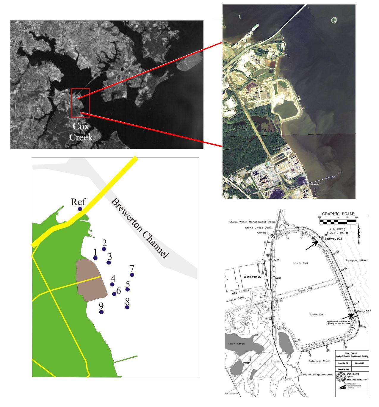
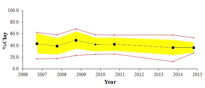
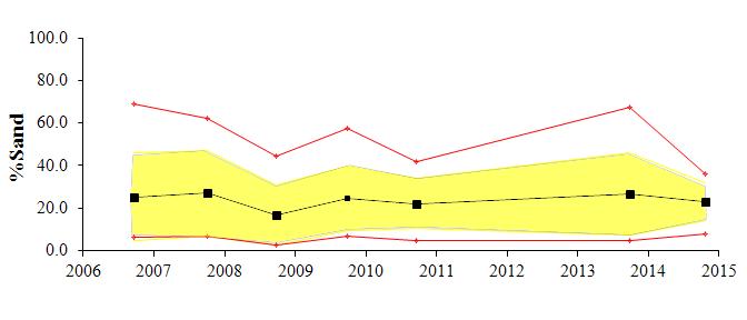
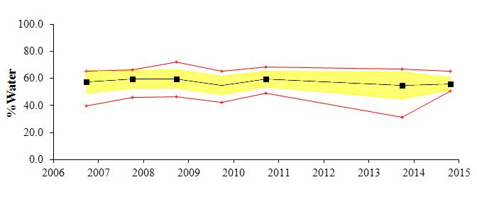
The textural component summary statistics for the study area for the past several monitoring years (2006-2014) are presented graphically in Figure 2. The average for each parameter is shown by a black line, the standard deviation by the yellow shading and the maximum and minimum values by the red line. Generally the area is comprised of fine grained sediments; with approximately 35-40% clay, 30-35% silt, and 15-20% sand content. There has been little change in the overall (average) textural parameters over all monitoring years. The depositional environment appears to be very stable.
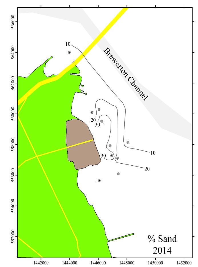
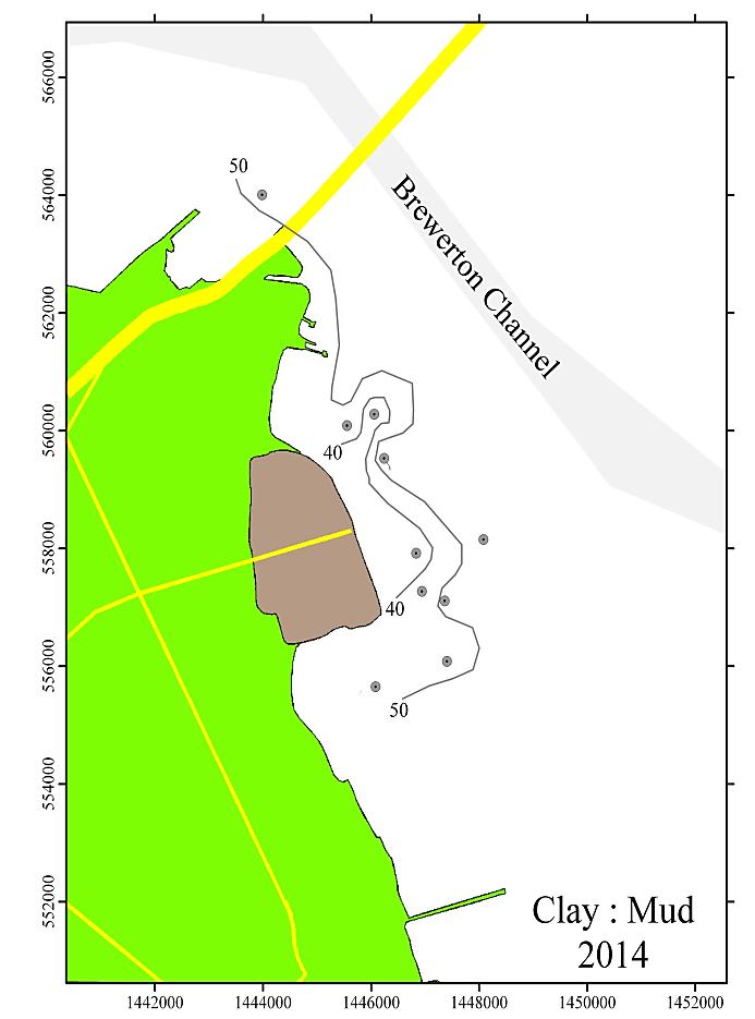
Figures 3 and 4 show the 2014 distribution of the grain size as the percent sand and the clay to mud ratio (CMR; %clay / [%silt + %clay]). The distribution pattern shows coarser sediments grading to finer ones proceeding from the containment area to the shipping channel and downstream. This is demonstrated by the sand content, which decreases from approximately 30% to less than 10%. The CMR increases from >40% to <50% toward the channel and in the downgradient direction. Silt-rich sediments (clay:mud ratio < 0.50) are generally found immediately adjacent to the walls of the dike, and clay-rich sediments (clay:mud ratio > 0.50) are generally found further downgradient, similar to distribution pattern seen at HMI DMCF.
13 Percent Enriched or Depleted -39 +120 +130 +71 -50 -18 +200 +110 Std Deviations from the HMI Baseline, in % 61 23 27 22 43 29 21 30 Sigma levels for CCE-07 -0.7 5.2 4.8 3.2 -1.2 -0.6 9.6 3.7
There has been only subtle variation in the gross data between the seven years. During monitoring years 2006, 2008, and 2010, sediments were relatively fine grained, with the sand content maximum of approximately 40% decreasing to less than 10% with distance. During monitoring years 2007, 2009, and 2013, sediments coarsened, with the sand content maximum of approximately 50% -60%, decreasing to less than 10% with distance. No data was collected in 2011 or 2012. During this most recent monitoring year, sediments were finer-grained, with the maximum percent sand of approximately 30%. A similar trend is seen with the CMR distribution, indicating that fining is due to slight increase in silt.
The reference station has exhibited the largest shifts in grain size over the years, with sand varying from greater than 70% in 2006 to less than 10% in 2008. Sand content for the reference station for this year was 12%. The CMR at this station increased slightly, from just less than 50% in 2013 to 53% this year
14
(black line), standard deviation (yellow shading) and the minimum and maximum values (red lines) for the sand,
15
Figure 2:Trend plots of textural components of the exterior sediments collected around Cox Creek DMCF. Plots show the average
silt and clay components for each of the monitoring years. Exterior sediment monitoring began in 2006.


16
Figure 3: Distribution of % Sand in the Cox Creek study area for the 2014 monitoring year.
Figure 4: Distribution of the Clay : Mud ratio in the Cox Creek study area for the 2014 monitoring year.
Carbon, Nitrogen, Phosphorus, and Sulfur
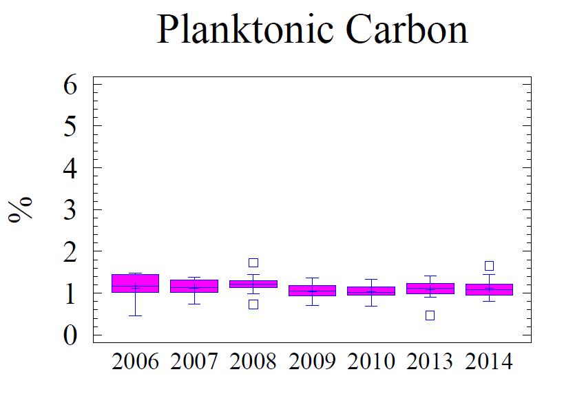
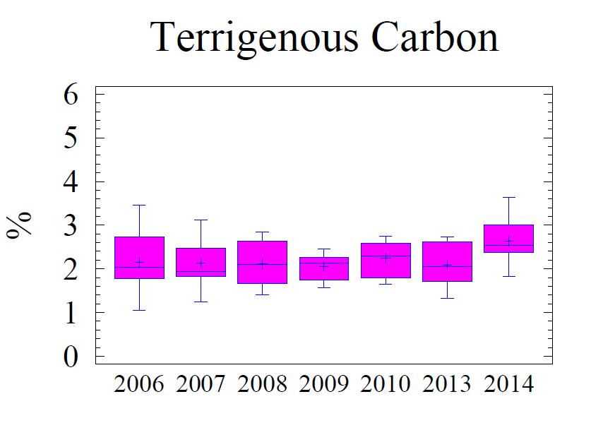
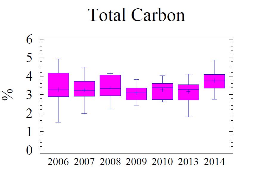
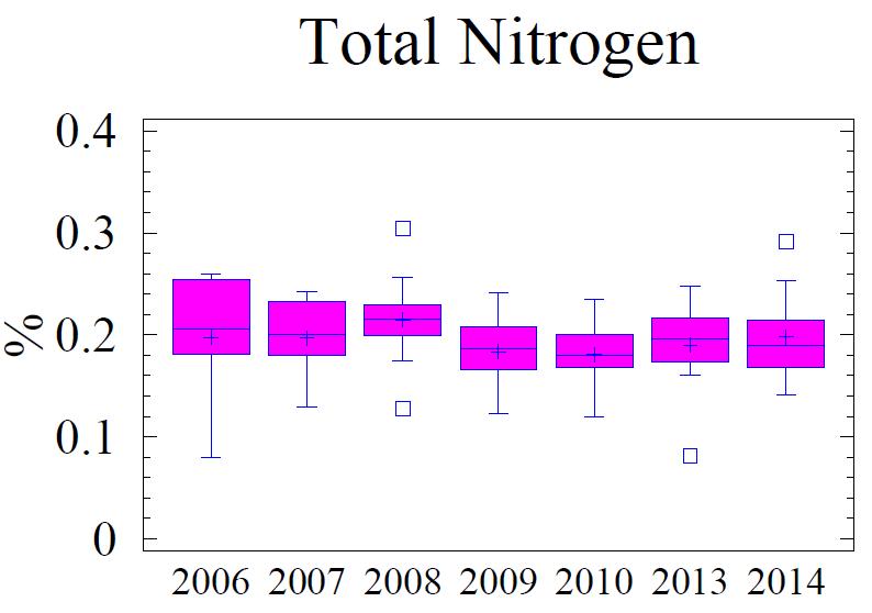
Sedimentary C, N, P, and S are indicators of the geochemical depositional environment. The concentration of C, N, P, and S in the sediment is related to the grain size; higher concentrations of these elements are found associated with fine grain sediments, specifically clay size minerals (Table 5). Total C (referred to as “C” in this discussion) in the sediment is comprised of planktonic C (Cplanktonic) and terrigenous C (Cterrigenous). Cplanktonic is organic detritus from primary production in the water column. It is derived from plankton that has a molar ratio of 16:106 (N:C) based on the work of Redfield et al. (1963). Cterrigenous is organic material from land run-off, coal from mining, and industrial sources; Cterrigenous has virtually no N content (Hennessee et al., 1986). Consequently, by using the N content with Redfield’s ratio 16:106 (N:C) the terrigenous component can be separated from the planktonic component via a mixing equation. Figure 5 presents the statistical behavior of different measured and calculated fractions of C; Cterrigenous, and Cplanktonic for the monitoring history (2006 -2014). The Cplanktonic, based on the measured N content (see Figure 6) and the Redfield ratio, is consistent with findings in the central portion of the Baltimore Harbor outside of the main shipping channel. This is expected due to the relative uniformity of the environmental conditions. Factors that affect water column productivity and the settling of the detritus from the plankton do not vary significantly; i.e. there is very little difference in the water column chemistry, the water depths, proximity to land, or hydrodynamic setting to warrant major differences. Consequently, N is similar to the central portion of the Harbor and by extension so is the fraction Cplanktonic The fraction Cterrigenous, calculated as total C minus Cplanktonic, is significantly higher in the vicinity of Cox Creek compared to further into the Harbor. Cox Creek DMCF is close to Sparrow’s Point and the mouth of the Harbor, both of which are potential sources of Cterrigenous originating from coal; either from industrial usage or from the upper Bay which receives a significant amount of coal from mining along the Susquehanna River (Hennessee et al., 1986; Hill et al. 2001). The Cterrigenous input is greater than primary productivity (Cplanktonic).
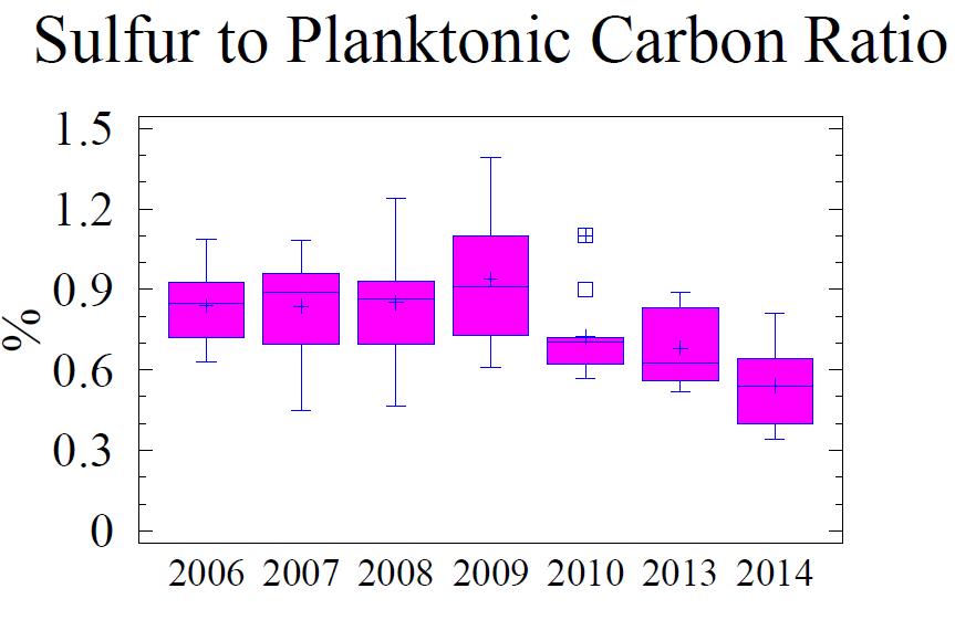
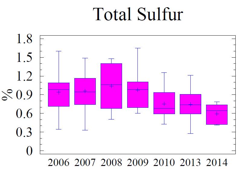
Sedimentary S differs from N, C and P in that its formation and burial in sediments is predominantly a result of bacterially mediated diagenetic reactions between sulfate in the water column and reactive C in the sediment. The ultimate result is the depletion in C content and the production of metal sulfide minerals in the sediment (Berner, 1970). The amount of sulfide found in the sediment is a result of several factors including the initial amount of reactive C (principally Cplanktonic), transport-related factors allowing for movement of sulfate into the sediment, and the length of time the sediment interacts with the water column. The latter is determined by the sedimentation rate and biological mixing. An indicator of the progress of this process is the S:C ratio; the higher the ratio, the more C consumed in the production of sulfide minerals. Figure 6 shows two S:C ratios; the ratio using total S and C, and the ratio using Cplanktonic (to reflect the amount of reactive C in the sediment). At Cox Creek, the total amount of sedimentary sulfur and both S:C ratios declines slightly over time, whereas the total amount of sedimentary carbon remains constant. Generally, the S:Cplanktonic is within the range typical of mid-Bay samples while the S:C is low. The relatively high proportion of Cterrigenous accounts for the low S:Ctotal ratios.
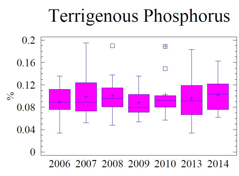
Although total P does not directly undergo reduction-oxidation processes in sediments, its cycling within the Chesapeake Bay is controlled by the redox state of certain elements, particularly Fe, Mn, and S, and by the concentration of organic material (C). Sources of P include weathering of natural soils and rocks, urban and agricultural runoff, and discharges from wastewater treatment plants Phosphate (PO4 -3) from fertilizers binds to soils, which erode during storm events, adding considerable amounts of suspended phosphate to streams that flow into the Bay. Municipal waste-
17
water discharge, which discharges phosphate as orthophosphate and organic phosphorus, is a major source of P to the Chesapeake Bay (Chesapeake Bay Program, 2009) Unlike N and C, P has no gaseous form. Therefore, P is not cycled out of the system like N is by way of denitrification or C is by respiration. Thus P tends to accumulate in the sediments. Once in the sediments, P is slowly released into the interstitial water as organic material is oxidized. Free phosphate is rapidly bound to ferric oxyhydroxides and oxidized manganese which are found in the upper, oxidized layer of the sediments (i.e., oxidized flocculant layer on sediment surface). Deeper in the sediment column where anoxic conditions prevail and metals oxides have been reduced, P is released into the interstitial water and, if sulfide is low or absent, reacts with reduced forms of metals, particularly Fe, forming hydrous phosphates (i.e., vivianite, vivianite group). However, if present, free sulfide will bind more readily to the reduced Fe and the phosphate remains free to diffuse upward to the oxidized layer where it is "captured" by excess ferric oxyhydroxides (FeOOH) and manganese oxides found in the upper sediment layer. If the overlying water column becomes anoxic, the “captured” P may be released in the overlying water column where it can contribute to increased algae/plankton production, and escape the sediments. The portion of total P active in this cycle includes the loosely sorbed phosphate; fresh, leachable, organic P, and iron-bound phosphate. These available forms of P make up 40% to 50% of the total P in the upper 1 cm of sediments and are largely depleted below 3 cm in the sediment column (Jorgensen, 1996). Any P below this depth usually consists of the more stable forms that are bound to clay minerals, associated with apatite or calcium carbonate minerals, and becomes permanently buried in the sediments.
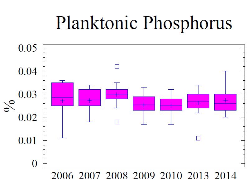
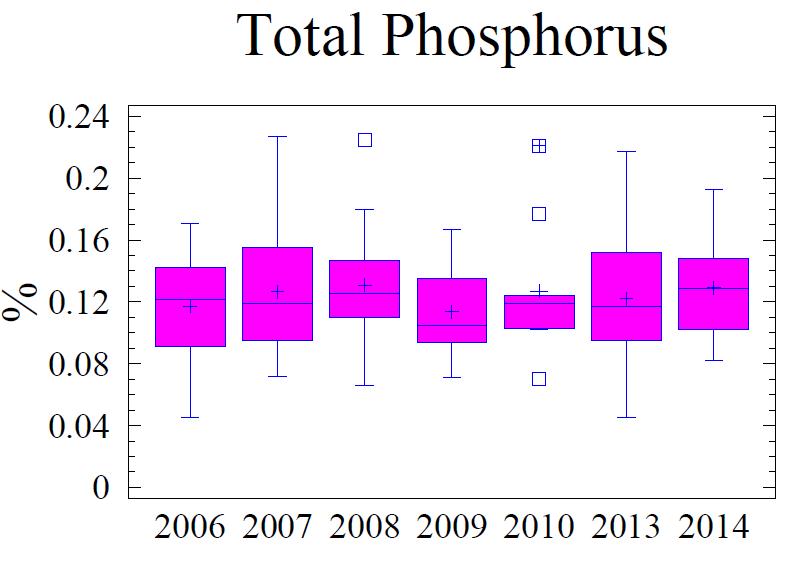
The fine-grained sediments adjacent to the Cox Creek DMCF contain an average of 0.12% total P, which is 30% to 40% higher than the sediments adjacent to Masonville DMCF and HMI DMCF (Table 6). Based on Redfield N:P ratio of 16:1, a small portion of the total P may be attributed to algae (Figure 7). However, 70% to 80% of the P is considered non-Redfield fraction which includes the loosely bound terrigenous forms of P and the more stable mineral forms.
Overall, C, N, P, and S data have not changed significantly from one monitoring year to another. This indicates a relatively stable depositional/geochemical environment adjacent to the DMCF.
18
Table 5. Correlation matrix for textural, nutrient and target metal data based on all of the sediment samples collected in 2014. The correlations were determined using a Pearson product-moment technique (Johnson and Wichern, 1982). Values listed in the table are Pearson correlation coefficients (r). Shaded values are statistically significant at the 95% confidence level (p < 0.05).
19
H2O SAND SILT CLAY N C S P_Perc Cd Cr Cu Fe_Perc Mn Ni Pb Zn As Hg H2O -0.73 0.03 0.77 0.91 0.23 0.42 0.45 0.86 0.65 0.74 0.43 0.03 0.70 0.82 0.57 0.47 0.46 SAND -0.73 -0.38 -0.87 -0.64 -0.22 -0.39 -0.34 -0.66 -0.72 -0.54 -0.42 0.12 -0.67 -0.66 -0.43 -0.33 -0.08 SILT 0.03 -0.38 -0.12 -0.07 0.27 -0.57 -0.09 0.88 0.34 -0.01 -0.03 -0.27 0.03 -0.14 -0.12 -0.17 -0.32 CLAY 0.77 -0.87 -0.12 0.73 0.09 0.70 0.45 0.57 0.62 0.60 0.50 0.01 0.71 0.80 0.56 0.47 0.27 N 0.91 -0.64 -0.07 0.73 0.46 0.34 0.66 0.87 0.76 0.92 0.59 0.14 0.76 0.92 0.75 0.76 0.61 C 0.23 -0.22 0.27 0.09 0.46 -0.36 0.56 0.03 0.56 0.59 0.42 0.44 0.45 0.40 0.53 0.65 0.52 S 0.42 -0.39 -0.57 0.70 0.34 -0.36 -0.08 0.58 -0.03 0.10 -0.02 -0.17 0.19 0.35 0.04 0.04 -0.06 P_Perc 0.45 -0.34 -0.09 0.45 0.66 0.56 -0.08 -0.28 0.76 0.82 0.96 0.67 0.88 0.82 0.98 0.85 0.81 Cd 0.86 -0.66 0.88 0.57 0.87 0.03 0.58 -0.28 0.77 0.76 -0.32 -0.98 0.17 0.64 0.01 0.27 -0.62 Cr 0.65 -0.72 0.34 0.62 0.76 0.56 -0.03 0.76 0.77 0.87 0.79 0.24 0.80 0.84 0.82 0.70 0.41 Cu 0.74 -0.54 -0.01 0.60 0.92 0.59 0.10 0.82 0.76 0.87 0.74 0.26 0.78 0.90 0.87 0.91 0.70 Fe_Perc 0.43 0.12 -0.03 0.50 0.59 0.42 -0.02 0.96 -0.32 0.79 0.74 0.67 0.91 0.81 0.96 0.72 0.66 Mn 0.03 0.12 -0.27 0.01 0.14 0.44 -0.17 0.67 -0.98 0.24 0.26 0.67 0.56 0.35 0.63 0.35 0.67 Ni 0.70 -0.67 0.03 0.71 0.76 0.45 0.19 0.88 0.17 0.80 0.78 0.91 0.56 0.89 0.91 0.69 0.68 Pb 0.82 -0.66 -0.14 0.80 0.92 0.40 0.35 0.82 0.64 0.84 0.90 0.81 0.35 0.89 0.90 0.77 0.63 Zn 0.57 -0.43 -0.12 0.56 0.75 0.53 0.04 0.98 0.01 0.82 0.87 0.96 0.63 0.91 0.90 0.84 0.77 As 0.47 -0.33 -0.17 0.47 0.76 0.65 0.04 0.85 0.27 0.70 0.91 0.72 0.35 0.69 0.77 0.84 0.77 Hg 0.46 -0.08 -0.32 0.27 0.61 0.52 -0.06 0.81 -0.62 0.41 0.70 0.66 0.67 0.68 0.63 0.77 0.77
Figure 5. Box and whisker diagrams showing range and distribution of total C, Cplanktonic and Cterrigenous, for the monitoring years 2006 through 2014. Box and whisker diagrams provide graphical representations of the dispersion of points within data sets. The data for each year are divided into four areas of equal frequency, with a box enclosing the middle 50 percent. The median is drawn as horizontal line and mean as a ‘plus sign’ inside the box. Vertical lines, known as whiskers, extend from upper and lower ends of the box. The lower whisker is drawn from the first quartile to the smallest point within 1.5 interquartile ranges from the lower quartile. The upper whisker is drawn from the upper quartile to the largest point within 1.5 interquartile ranges from the upper quartile; values that fall beyond the whiskers but within 3 interquartile ranges are plotted as individual points. Those values are suspect outliers. Near outliers are plotted as a box, and far outliers as plotted as a box with “+” sign.
20
Figure 6 Box and whisker diagrams showing range and distribution of total S and N and the ratios of S:C and S:Cplanktonic for the monitoring years 2006 through 2014. Refer to Figure 5 for explanation of the box and whisker diagram symbols.
21
Figure 7. Box and whisker diagrams showing range and distribution of total P, Pterrigenous and Pplanktonic for the monitoring years 2006 through 2014. Refer to Figure 5 for explanation of the box and whisker diagram symbols.
22
Target Metals
The concentrations of the target metals of interest are high, as would be expected in fine grain northern Chesapeake Bay sediments in the Baltimore Harbor. The summary statistics for the samples in the Cox Creek study area are given in Tables 7 and 8 (for Hg), along with the Effects Range Low (ERL) and Effects Range Median (ERM) threshold values (Buchman, 2008) for reference. Briefly, the ERL and ERM threshold values are considered screening values for evaluating potential toxicological effects from contaminant concentrations in sediments. Concentrations measured at some stations during the 2014 monitoring year were above the ERL for Cr, Cu, Hg, Ni, Pb and Zn. Concentrations measured at some stations during the 2014 monitoring year were above the ERM for Cu, Hg, Ni, and Zn Please note that there are no ERLs or ERMs for Fe and Mn. The 2014 results are generally consistent with the previous monitoring years
As discussed in Discussion-Target Metal Regional Baseline section of this report, the more appropriate way of viewing the data is in the context of the metals concentrations normalized to the grain size data for the main stem of the Chesapeake Bay. All previous monitoring years have shown elevated levels of Cr, Cu, Pb, and Zn with respect to the northern Chesapeake Bay reference levels.
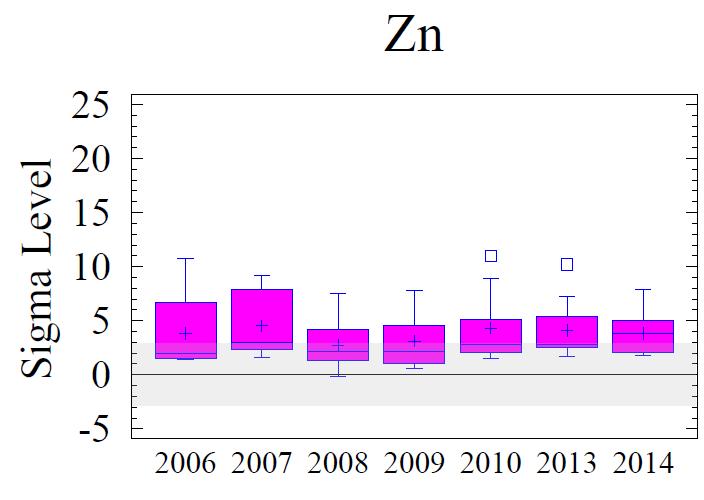
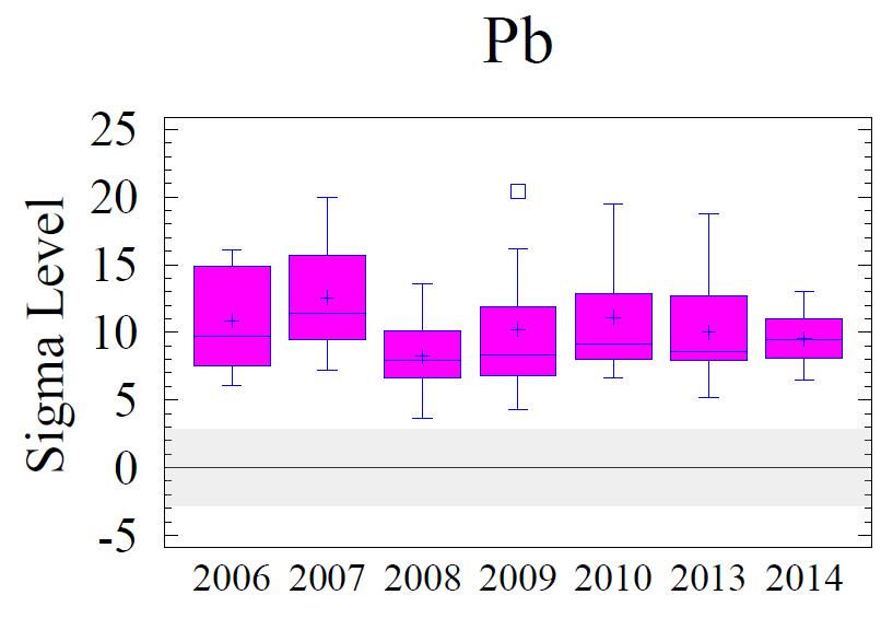
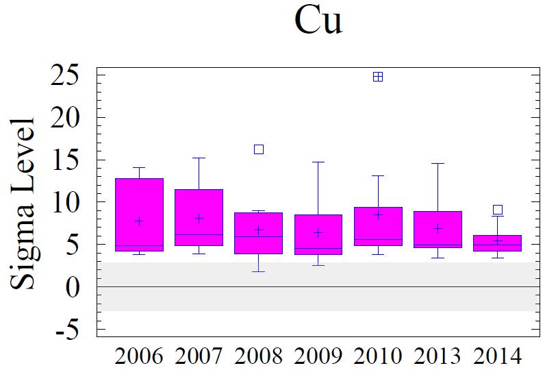
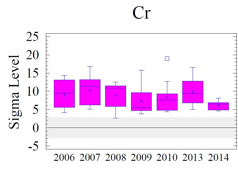
Figure 8 shows box and whisker diagrams for the sigma values of the elevated metals for all of the sampling sites for all six monitoring years. Samples within + or - 2 sigma are considered within the regional background levels; 3 sigma is borderline; and greater than 3 sigma is considered to vary from the regional baseline with statistical significance. The data in the figure show minor variations from year to year; however, Cr, Cu, Pb and Zn remain elevated above background concentrations.
23
Clay% N% C% S% P% S:C ratio Baltimore Harbor (1995-96) 49.35 0.310 4.170 0.900 Not analyzed 0.216 HMI DMCF (2014) 43.44 0.189 2.565 0.367 0.068 0.143 Masonville DMCF (2014) 36.86 0.179 2.827 0.892 0.086 0.316 Cox Creek DMCF (2014) 36.74 0.198 3.758 0.593 0.129 0.158
Table 6. Comparison of the average amount of clay content, major nutrients, and sulfur contents in the sediments in the Baltimore Harbor and adjacent to the three DMCFs located in the Baltimore Harbor region.
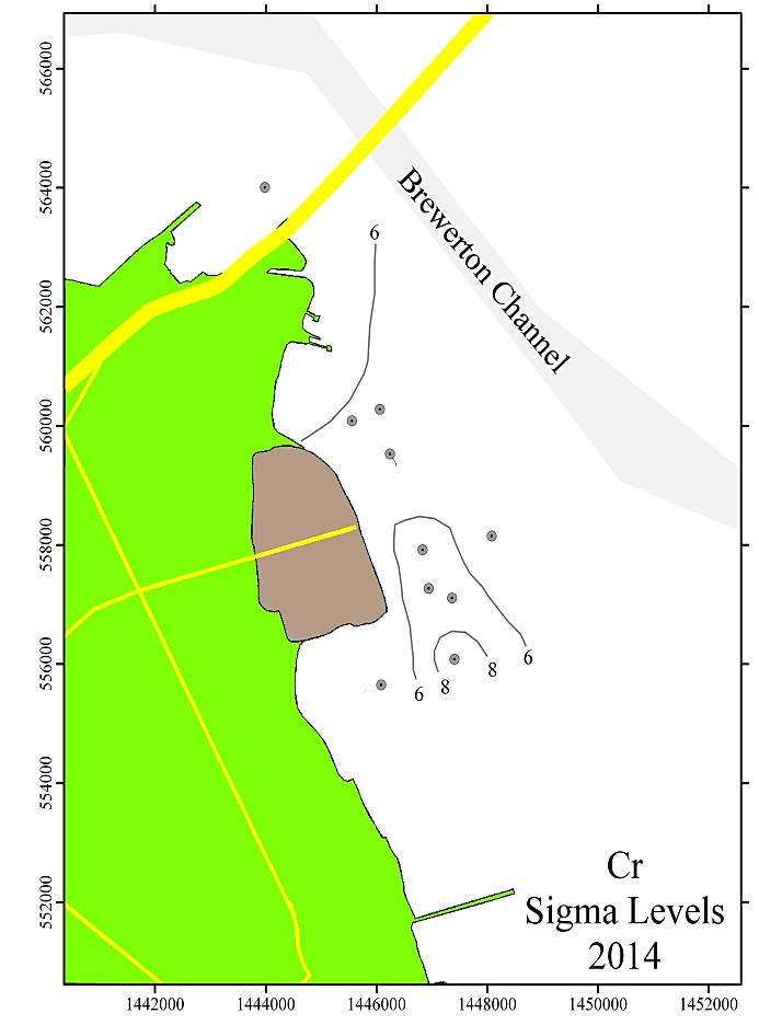
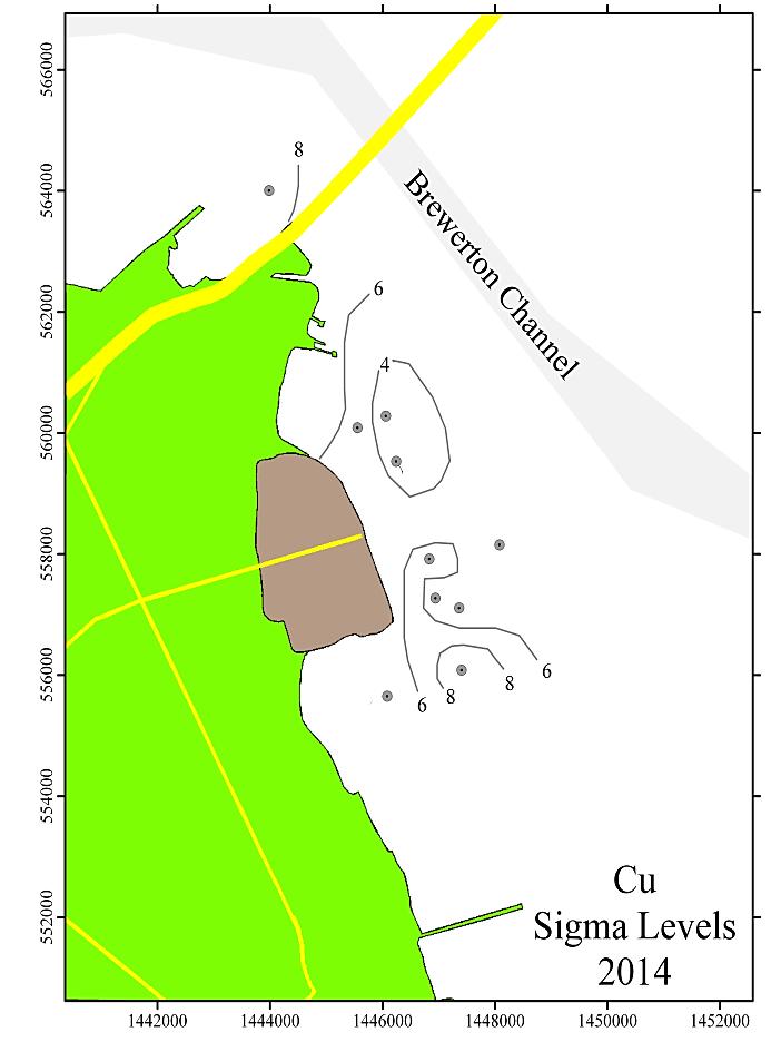
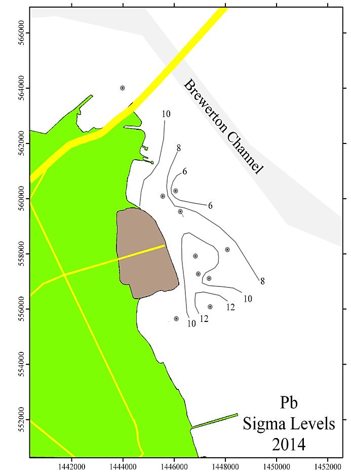
Figure 9 shows the spatial distribution of the sigma values for Cr, Cu, Pb, and Zn for the Cox Creek DMCF study area for the 2014 sampling. The contours shown are in increments of 2 sigma.
Table 7. Summary statistics for target metals for monitoring years 2006 through 2014. Included for reference are the ERL and ERM values from Buchman (2008). Values are in ppm unless otherwise indicated. For emphasis, the number of samples with values exceeding ERLs or ERMs is shaded.
24
Statistic 2006 2007 2008 2009 2010 2013 2014 2006 2007 2008 2009 2010 2013 2014 Cd Cr Ave. 0.8 1 1.4 0.8 1.1 0.6 0.53 292 301 318 261 289 290 225 std 0.2 0.2 0.4 0.4 0.5 0.2 0.19 88 60 83 96 112 82 33 Min. 0.3 0.7 0.9 0.4 0.7 < 0.3 <0.3 199 230 190 146 200 219 171 Max. 1.1 1.1 2.2 1.7 2.4 1.0 0.80 479 388 478 483 542 458 277 n 10 10 10 10 10 10 10 10 10 10 10 10 10 10 ERL 1.3 1.3 1.3 1.3 1.3 1.3 1.3 81 81 81 81 81 81 81 n>ERL 0 0 3 2 2 0 0 10 10 10 10 10 10 10 ERM 9.5 9.5 9.5 9.5 9.5 9.5 9.5 370 370 370 370 370 370 370 n>ERM 0 0 0 0 1 0 0 2 2 2 2 2 2 0 Cu Ni Ave. 117 113 118 106 130 104 90 57 53 61 50.8 54 48 49 std 41 27 43 46 75 46 24 17 9 9 7.9 7 9 6 Min. 53 77 73 63 75 47 63 27 34 46 36 43 28 39 Max. 200 157 201 212 316 190 137 81 64 73 62 68 63 60 n 10 10 10 10 10 10 10 10 10 10 10 10 10 10 ERL 34 34 34 34 34 34 34 21 21 21 21 21 21 21 n>ERL 10 10 10 10 10 10 10 10 10 10 10 10 10 10 ERM 270 270 270 270 270 270 270 52 52 52 52 52 52 52 n>ERM 0 0 0 0 1 0 1 8 6 8 6 7 2 1 Pb Zn Ave. 116 116 107 107.9 118 98 94 447 437 421 410 485 417 393 std 38 28 27 37.1 46 41 21 230 149 152 221 266 214 117 Min. 43 85 59 65 71 41 67 166 283 226 197 258 165 243 Max. 180 165 151 177 216 185 129 1040 811 757 813 1090 900 570 n 10 10 10 10 10 10 10 10 10 10 10 10 10 10 ERL 47 47 47 47 47 47 47 150 150 150 150 150 150 150 n>ERL 9 10 10 10 10 9 10 10 10 10 10 10 10 10 ERM 218 218 218 218 218 218 218 410 410 410 410 410 410 410 n>ERM 0 0 0 0 0 0 0 5 6 4 3 4 3 4 Fe (%) Mn Ave. 6.83 7.45 7.264 6.7 7.71 7.10 6.44 1447 1218 1302 1036 1229 950 1011 std 2.26 1.86 1.5367 2 2.20 2.03 1.14 515 268 213 205 163 219 224 Min. 3.72 4.92 4.67 4.37 5.29 3.91 5.00 427 563 978 810 997 555 725 Max. 12.1 11.4 10.5 10.4 12.50 11.30 8.04 2080 1540 1690 1390 1480 1340 1340 n 10 10 10 10 10 10 10 10 10 10 10 10 10 10 ERL n/a n/a n/a n/a n/a n/a n/a n/a n/a n/a n/a n/a n/a n/a n>ERL ERM n/a n/a n/a n/a n/a n/a n/a n/a n/a n/a n/a n/a n/a n/a n>ERM
Generally, levels of enrichment and spatial distribution for Cr, Cu, Pb, and Zn have not changed significantly from previous monitoring years. These data are depicted graphically and spatially as Figures 8 and 9 (following pages). A few observations to note:
1. The entire area is significantly enriched (above 3 sigma) for Cr, Cu, and Pb.
2. A portion of the area is significantly enriched for Zn. The affected area resembles the spatial distribution of the other metals, but is smaller in total area.
3. The pattern of the sigma contours for all elevated metals (including Fe, not shown) depicts the entire area of sediments adjoining the Cox Creek DCMF as enriched in these metals. Over time (2006-2014), there has been no observable increase in size of the area with metals enrichment nor has there been any upward trend in the magnitude of metals enrichment (as expressed in sigma levels) in the sediments adjacent to the facility
Table 8. Summary statistics for mercury for the Cox Creek DMCF area for the monitoring years 2008 through 2014. Mercury analysis using the cold vapor analytical method was not done in 2006 and 2007. Included for reference are the ERL and ERM values from Buchman (2008). For emphasis, the number of samples with values exceeding ERLs or ERMs are shaded.
In general, all monitoring years are comparable with minor variations. Over time, local concentration maxima, for each metal, have been observed at sampling stations 4, 6 and 8 (i.e. adjacent to the facility and extending to the southeast). Metals concentrations expressed as sigma levels actually decreased slightly in 2014, most notably for Cr and Cu. Spatial distribution patterns remain comparable to previous monitoring years. Although sedimentary enrichment is observed adjacent the Cox Creek DMCF dike, a similar spatial pattern has been observed since 2006, and metals enrichment does not show increasing spatial extent nor increasing magnitude of enrichment over time.
25
2008 2009 2010 2013 2014 Hg (ppb) Ave. 466 345 348 308 414 std 236 101 98 103 174 Min. 200 244 204 104 238 Max. 924 516 484 471 796 n 10 10 10 10 10 ERL 150 150 150 150 150 n>ERL 10 10 10 9 10 ERM 710 710 710 710 710 n>ERM 2 0 0 0 1
Figure 8. Box and whisker diagrams of the sigma levels for Cr, Cu, Pb, and Zn for monitoring years 2006 through 2014. Samples within + or - 2 sigma are within the regional background levels, +3 sigma is borderline, and greater than 3 sigma is statistically significantly influenced by local sources or processes. Background levels are depicted by the gray shaded area. All metals are statistically elevated above regional background. Refer to Figure 5 for explanation of the box and whisker diagrams.
26

27
Figure 9: Distribution of sigma levels for Cr, Cu, Pb, and Zn in the Cox Creek study area for the 2014 monitoring year. Contour levels are in increments of 2 sigma.
SUMMARY
1. Sediments around the Facility are generally fine grained and exhibit a gradient of higher sand content close to the dike, diminishing outwards toward the channel and downstream This distribution pattern has been reproducible during all monitoring years.
2. As derived from the total N and total P content of the sediment, the sediments adjoining the Cox Creek DMCF study area receive the majority of their organic matter from terrigenous sources as opposed to planktonic sources.
3. The sulfur to carbon (S:C) ratio is lower than that measured further into the Harbor, indicating that the area is slightly more disturbed or has a higher sedimentation rate than further into the Harbor.
4. Certain target metals, including Cd, Mn, and Ni, remain within background levels found in the northern Chesapeake Bay. The remaining target metals, including Cr, Cu, Fe, Pb and Zn, are elevated above regional background levels. Forty percent of the sampling sites are enriched with respect to Zn. Ninety to 100 percent of the sites were significantly enriched with Cr, Cu, Fe, Pb.
5. Target metals in the study area follow the general pattern seen in the 1994 - 1997 Baltimore Harbor study (Baker et al, 1997 and references within.) The sediments exterior to the Cox Creek DMCF appear enriched in Fe and Pb, and to a lesser extent, in Cr, Cu and Zn relative to some, but not all, areas of Baltimore Harbor.
6. Physically and chemically, the reference site is not representative of sediments immediately exterior to the DMCF. Large variations in sediment texture have occurred at the reference site; for example the % sand has ranged more than 50% (from >60% in 2007 to < 10% in 2008) and the clay-to-mud ratio (CMR) ranged more than 20%. The reference site helps provide spatial coverage which suggest additional external source of regional metals, but may not be a good gauge to measure changes due to operation of the DMCF. Therefore changes due to operation of the DMCF are best evaluated through monitoring any changes to the exterior sediments over time.
7. The spatial pattern of the metals concentrations, expressed as sigma level contours, for all elevated metals (Cr, Cu, Pb and Zn) depicts the entire area of sediments adjoining the Cox Creek DCMF as significantly enriched in these metals. The local sigma maximum was observed at sampling station #8 during the 2014 event, located to the southeast of the DMCF, consistent with most preceding monitoring years. Over time (2006-2014), there has been no observable increase in size of the area with metals enrichment nor has there been any upward trend in the magnitude of metals enrichment (as expressed in sigma levels) in the sediments adjacent to the facility. We interpret the stability of spatial pattern, size and magnitude as indicative of no outward effects from the Cox Creek DMCF operations to the exterior sedimentary environment.
28
REFERENCES
Baker, J., Mason, R., Cornwell, J., Ashley, J., Halka, J. and Hill, J.M., 1997, Spatial Mapping of Sedimentary Contaminants in the Baltimore Harbor/Patapsco River/Back River Systems. Final Report Submitted to Maryland Department of the Environment. Contract No. P.O.
UOOP6002389: Ref No. UMCES [CBL] 97-142
Berner, R.A., 1970, Sedimentary Pyrite Formation, Am. J. Science, vol. 268, p. 1- 23
Blatt, H., Middleton, G., and Murray, R., 1980, Origin of Sedimentary Rocks: Englewood Cliffs, NJ, Prentice-Hall, Inc., 782 p.
Buchman, M.F., 2008, NOAA Screening Quick Reference Tables, NOAA OR&R Report 08-1, Seattle WA, Office of Response and Restoration Division, National Oceanic and Atmospheric Administration, 34 p.
Chesapeake Bay Program, 2009, Chesapeake Bay Program Phase 4.3 Watershed Model 2007 Simulation,
Helz, G.R., Sinex, S.A., Serlock, G.H., and Cantillo, A.Y., 1982, Chesapeake Bay sediment trace elements: Final Report to U.S. Environmental Protection Agency, Grant No. R805954, Univ. of Maryland, College Park, Md., 202 pp.
Hennessee, E.L., Blakeslee, P.J., and Hill, J.M., 1986, The distribution of organic carbon and sulfur in surficial sediments of the Maryland portion of the Chesapeake Bay, J. Sed. Pet., v. 56, p. 674-683.
Hennessee, L., Hill, J.M., and Park, J. 1995, Sedimentary environment, in Assessment of the Environmental Impacts of the Hart and Miller Island Containment Facility: 12th Annual Interpretive Report Aug. 92 - Aug. 93: Annapolis, MD, Maryland Dept. of Natural Resources, Tidewater Admin.
Hill, J.M., 1988, Physiographic Distribution of Interstitial Waters in Chesapeake Bay. Maryland Geological Survey Report of Investigation No. 49, 32 pp.
Hill, J.M., 2007, Cox Creek Exterior Sedimentary Environment Baseline Study 2006. Maryland Geological Survey, Coastal and Estuarine Geology Program File Report 07-04, 31 pp.
Hill, J.M., 2008, Cox Creek Dredge Material Containment Facility Exterior Monitoring: Sedimentary Environment 2007. Maryland Geological Survey, Coastal and Estuarine Geology Program File Report 08-03, 33 pp.
Hill, J.M., VanRyswick, S., and Wells, D., 2009, Cox Creek Dredge Material Containment Facility Exterior Monitoring: Sedimentary Environment 2008. Maryland Geological Survey, Coastal and Estuarine Geology Program File Report 09-07. 39 pp.
Hill, J.M., Wikel, G., Bethke, T., Wells, D., Mason, R., Baker, J., Connell, D., Liebert, D., 2001, Characterization of Bed Sediment Behind the Lower Three Dams on the Susquehanna River
29
Maryland Geological Survey, Coastal and Estuarine Geology Program File Report 01-5
Johnson, R.A. and Wichern, D.W., 1982, Applied multivariate statistical analysis: New Jersey, Prentice-Hall.
Jorgensen, B.B., 1996, Material flux in the sediment, in Jorgensen, B.B, and Richardson, K., (eds.) Eutrophication in Coastal Marine Ecosystems. Coastal and Estuarine Studies Vol 52, Amer. Geophysical Union, Washington, DC, p. 115-135.
Kerhin, R.T., Halka, J.P., Wells, D.V., Hennessee, E.L., Blakeslee, P.J., Zoltan, N., and Cuthbertson, R.H., 1988, The Surficial Sediments of Chesapeake Bay, Maryland: Physical Characteristics and Sediment Budget: Baltimore, MD, Maryland Geol. Survey Report of Investigations No. 48, 82 p.
Kerhin, R.T., Hill, J., Wells, D.V., Reinharz, E., and Otto, S., 1982a, Sedimentary environment of Hart and Miller Islands, in Assessment of the Environmental Impacts of Construction and Operation of the Hart and Miller Islands Containment Facility: First Interpretive Report
Kerhin, R.T., Reinharz, E., and Hill, J., 1982b, Sedimentary environment, in Historical Summary of Environmental Data for the Area of the Hart and Miller Islands in Maryland: Hart and Miller Islands Special Report No. 1: Shady Side, MD, Chesapeake Research Consortium, p. 10-30.
Kotulak, P.W. and Headland, J. R., 2007, Cox Creek Dredged Material Containment Facility design and construction: Ports 2007: 30 Years of Sharing Ideas…1977-2007. Proceedings of the Eleventh Triennial International Conference, ASCE, v. 238, p. 1-10.
Mason, R.P., and Lawrence, A.L., 1999, Concentration, Distribution and Bioavailability of Mercury and Methylmercury in Sediments of Baltimore Harbor and Chesapeake Bay, Maryland, USA, Environmental Toxicology and Chemistry, v. 18(11), p 2438-2447.
Mason, R.P., Kim, E., and Cornwell, J. 2004, Metal accumulation in Baltimore Harbor: current and past inputs, Applied Geochemistry, v. 19, p. 1801-1825.
Marquardt, D.W., 1963, An Algorithm For Least Squares Estimation Of Nonlinear Parameters: Jour. Soc. Industrial and Applied Mathematics, v. 11, p. 431-441.
Maryland Environmental Service (MES), 2010, September 2010 Monthly Update 189: Metals and pH Treatment at HMI and Cox Creek, Oct. 1, 2010.
Pejrup, M., 1988, The Triangular Diagram Used For Classification Of Estuarine Sediments: A New Approach, in de Boer, P.L., van Gelder, A., and Nio, S.D., eds., Tide-Influenced Sedimentary Environments and Facies: Dordrecht, Holland, D. Reidel Publishing Co., p. 289300.
Redfield, A.C., Ketchum, B.H., and Richards, F.A., 1963, The influence of organisms on the composition of sea-water, in Hill, M.N. (ed.), The sea, volume 2, The composition of sea-water, comparative and descriptive oceanography: London, Interscience, p. 26-77.
30
Shepard, F.P., 1954, Nomenclature based on sand-silt-clay ratios: Journal of Sedimentary Petrology, v. 24, p. 151-158.
Sinex, S.A., and Helz, G.R., 1981, Regional geochemistry of trace elements in Chesapeake Bay sediments: Environ. Geol., vol. 3, p. 315-323.
Sylvia, E., VanRyswick, S., and Wells, D.V., 2014, The Continuing State Assessment of the Environmental Impacts of Construction and Operation of the Hart-Miller Island Containment Facility: Project II-Sedimentary Environment Thirty-Second Year Data Report (September 2013 - August 2014), Maryland Geological Survey, Coastal and Environmental Geosciences File Report 14-02, 35 pp.
Wells, D., and VanRyswick, S., 2011, Cox Creek Dredge Material Containment Facility Exterior Monitoring: Sedimentary Environment 2009: Baltimore, Md., Maryland Geological Survey, Coastal and Estuarine Geology File Report No. 11-01, 42 p.
Wells, D.V., Sylvia, E., and Van Ryswick, S., in prep., Appendix I-Sedimentary Environment (Project II) in MDE (in review ), Assessment of Impacts from the Hart-Miller Island Dredged Material Containment Facility, Maryland: Year 32 Exterior Monitoring Technical Report (September 2013-June 2014).
Wells, D.V.,Van Ryswick, S., and Sylvia, E., 2012, Cox Creek Dredge Material Containment Facility Exterior Monitoring: Sedimentary Environment 2010, Maryland Geological Survey, Coastal and Environmental Geosciences File Report 12-05, 43 pp.
Wells, D.V., and Sylvia, E., 2015, Masonville Dredge Material Containment Facility Exterior Sedimentary Environment 2013, Maryland Geological Survey, Coastal and Environmental Geosciences File Report 15-02, [in review].
31
32
Appendix A
Sample Location Coordinates
A-1
A-2
Location Date Sampling Locations (Maryland State Plane-NAD 83) Water Depth (Ft) Northing (ft) Easting (ft) CCE-REF 10/21/2014 564006 1443986 19.1 CCE-01 10/21/2014 560087 1445559 12.2 CCE-02 10/21/2014 560278 1446064 10.2 CCE-03 10/21/2014 559532 1446247 12.1 CCE-04 10/21/2014 557920 1446837 11.8 CCE-05 10/21/2014 557110 1447365 13.2 CCE-06 10/21/2014 557271 1446944 11.3 CCE-07 10/21/2014 558151 1448082 19.3 CCE-08 10/21/2014 556084 1447408 12.1 CCE-09 10/21/2014 555652 1446088 7.6
Table A-1. Date, location coordinates, and water depths for sediment samples collected in Fall 2014. Samples were collected by MES staff.
Appendix B
Summary of elemental analyses methods and QA/QC for ancillary elements analysis
B-1
Elements (Analytes) reported for this study include nine target metals (shaded) and 40 additional elements analyzed by Actlabs and three by MGS (C, N and S) (Table B-1). Sulfur was analyzed by both MGS and Actlabs using different methods.
Table B-1 Summary of analytical methods and detection limits. Methods abbreviations: High Temp. Combustion-GC - High Temperature combustion, following by Gas Chromatography; TD-ICP - Total Digestion followed by Inductively Coupled Plasma Spectrometry; INAA - Instrumental Neutron Activation Analysis; Hg-FIMS - aqua regia digestion followed by cold vapor FIMS analysis
B-2
Symbol Element Unit Detection Limit Analysis Method Analysis Laboratory N Nitrogen % 0.001 High Temp. Combustion-GC MGS C Carbon % 0.001 High Temp. Combustion-GC MGS P Phosphorus % 0.001 TD-ICP Actlabs S Sulfur % 0.001/0.01 High Temp. Combustion-GC/TD-ICP MGS/Actlabs Cd Cadmium ppm 0.3 TD-ICP Actlabs Cr Chromium ppm 2 INAA Actlabs Cu Copper ppm 1 TD-ICP Actlabs Fe Iron % 0.01 INAA Actlabs Hg Mercury ppb 5 Hg-FIMS Actlabs Mn Manganese ppm 1 TD-ICP Actlabs Ni Nickel ppm 1 INAA / TD-ICP Actlabs Pb Lead ppm 3 TD-ICP Actlabs Zn Zinc ppm 1 INAA / TD-ICP Actlabs As Arsenic ppm 0.5 INAA Actlabs Au Gold ppb 2 INAA Actlabs Be Beryllium ppm 1 TD-ICP Actlabs Sb Antimony ppm 0.1 INAA Actlabs Se Selenium ppm 3 INAA Actlabs Al Aluminum % 0.01 TD-ICP Actlabs Ag Silver ppm 0.3 INAA / TD-ICP Actlabs Ba Barium ppm 50 INAA Actlabs Bi Bismuth ppm 2 TD-ICP Actlabs Br Bromine ppm 0.5 INAA Actlabs Ca Calcium % 0.01 TD-ICP Actlabs Ce Cerium ppm 3 INAA Actlabs Co Cobalt ppm 1 INAA Actlabs Cs Cesium ppm 1 INAA Actlabs Eu Europium ppm 0.2 INAA Actlabs Hf Hafnium ppm 1 INAA Actlabs Ir Iridium ppb 5 INAA Actlabs K Potassium % 0.01 TD-ICP Actlabs La Lanthanum ppm 0.5 INAA Actlabs Lu Lutetium ppm 0.05 INAA Actlabs Mg Magnesium % 0.01 TD-ICP Actlabs Mo Molybdenum ppm 1 TD-ICP Actlabs
Table B-1 (cont.) Summary of analytical methods and detection limits. Methods abbreviations: High Temp. Combustion-GC - High Temperature combustion, following by Gas Chromatography; TD-ICP - Total Digestion followed by Inductively Coupled Plasma Spectrometry; INAA - Instrumental Neutron Activation Analysis; Hg-FIMS - aqua regia digestion followed by cold vapor FIMS analysis
B-3
Symbol Element Unit Detection Limit Analysis Method Analysis Laboratory Nd Neodymium ppm 5 INAA Actlabs Rb Rubidium ppm 15 INAA Actlabs Sc Scandium ppm 0.1 INAA Actlabs Sm Samarium ppm 0.1 INAA Actlabs Sn Tin % 0.01 INAA Actlabs Sr Strontium ppm 1 TD-ICP Actlabs Ta Tantatum ppm 0.5 INAA Actlabs Tb Terbium ppm 0.5 INAA Actlabs Ti Titanium % 0.01 TD-ICP Actlabs Th Thorium ppm 0.2 INAA Actlabs U Uranium ppm 0.5 INAA Actlabs V Vanadium ppm 2 TD-ICP Actlabs W Tungsten ppm 1 INAA Actlabs Y Yttrium ppm 1 TD-ICP Actlabs Yb Ytterbium ppm 0.2 INAA Actlabs
Table B-2. Results of all elemental analyses, including ancillary elements, of NIST SRM 1646a compared to the certified or known values, if available. Actlabs’ values were obtained by averaging the results of all SRM analyses run with the exterior sediment samples collected in Fall 2014 at Cox Creek, Masonville, and HMI DMCFs.
B-4
Element Unit ActLab’s Detection Limit Certified Values ActLab’s Result RSD % Recovery Mean Std. Dev. Ag ppm 0.3 < 0.3 Al % 2 2.405 0.021 0.88 104.7 As ppb 0.01 2.297 10 0.990 9.90 160.5 Au ppm 0.5 6.23 < 2 Ba ppm 50 < 50 Be ppm 1 < 1 Bi ppm 2 < 2 Br ppm 0.5 52.60 0.990 1.88 Ca % 0.01 0.519 0.555 0.007 1.27 106.9 Cd ppm 0.3 0.148 < 0.3 Ce ppm 3 29.50 2.121 7.19 Co ppm 1 6.50 0.707 10.88 Cr ppm 2 40.9 43.5 3.536 8.13 106.4 Cs ppm 1 < 1 Cu ppm 1 10.01 9.0 0.000 0.00 89.9 Eu ppm 0.2 0.50 0.283 56.57 Fe % 0.01 2.008 1.985 0.007 0.36 98.9 Hf ppm 1 12.00 1.414 11.79 Hg ppb 5 40 28 70.0 Ir ppb 5 < 5 K % 0.01 0.864 0.79 0.007 0.90 90.9 La ppm 0.5 18.55 0.071 0.38 Li ppm 1 18 17 0.000 0.00 Lu ppm 0.05 Mg % 0.01 0.388 0.37 0.000 0.00 95.4 Mn ppm 1 234.5 245.5 2.121 0.86 104.7 Mo ppm 1 2.50 0.707 28.28 Na % 0.01 0.741 0.725 0.007 0.98 97.8 Nd ppm 5 20.00 11.314 56.57 P % 0.001 0.027 0.026 0.000 0.00 96.3 Pb ppm 3 11.7 8.0 0.000 0.00 68.4 Rb ppm 15 < 15 S % 0.01 0.352 0.34 0.000 0.00 96.6 Sb ppm 0.1 0.30
NIST SRM 1646a- Estuarine Sediment
B-5
Element Unit ActLab’s Detection Limit Certified Values ActLab’s Results RSD % Recovery Mean Std. Dev. Sc ppm 0.1 4.55 0.354 7.77 Se ppm 3 0.193 < 3 Sm ppm 0.1 2.60 0.424 16.32 Sn % 0.01 < 0.01 Sr ppm 1 72 0.000 0.00 Ta ppm 0.5 < 0.05 Tb ppm 0.5 Th % 0.01 0.456 6.15 0.071 1.15 Ti ppm 0.2 0.48 0.000 0.00 105.3 U ppm 0.5 2.50 0.707 28.28 V ppm 2 44.84 46.50 0.707 1.52 103.7 W ppm 1 < 1 Y ppm 1 10 0.000 0.00 Yb ppm 0.2 Zn ppm 1 48.9 44.5 0.707 1.59 91.0
Table B-2, continued: NIST SRM 1646a- Estuarine Sediment
Table B-3. Results of all elemental analyses, including ancillary elements, of Canadian Research Council PACS-2 Marine Sediment compared to the certified or known values, if available. Actlabs’ values were obtained by averaging the results of all SRM analyses run with the exterior sediment samples collected in Fall 2014 at Cox Creek, Masonville, and HMI DMCFs.
CRC PACS-2 - Marine Sediment
B-6
Element Unit ActLab’s Detection Limit Certified Values ActLabs’ Result RSD % Recovery Mean Std. Dev. Ag ppm 0.3 1.22 1.2 0.141 11.79 98.4 Al % 2 6.585 0.049 0.75 99.5 As ppb 0.01 6.62 35.5 2.333 6.58 135.3 Au ppm 0.5 26.2 5.5 7.778 141.42 Ba ppm 50 710 141.421 19.92 Be ppm 1 1 1 0.000 0.00 100.0 Bi ppm 2 < 2 Br ppm 0.5 260 0.707 0.27 Ca % 0.01 1.96 2.07 0.007 0.34 105.4 Cd ppm 0.3 2.11 1.95 0.212 10.88 92.4 Ce ppm 3 36 8.485 23.57 Co ppm 1 11.5 16 0.707 4.56 134.8 Cr ppm 2 90.7 91.0 19.799 21.76 100.3 Cs ppm 1 < 1 Cu ppm 1 310 306 6.364 2.08 98.5 Eu ppm 0.2 0.5 0.636 141.42 Fe % 0.01 4.09 3.98 0.085 2.13 97.3 Hf ppm 1 2.000 2.828 141.42 Hg ppb 5 3.04 2640 86.8 Ir ppb 5 < 5 K % 0.01 1.24 1.16 0.014 1.22 93.5 La ppm 0.5 17.2 0.495 2.89 Li ppm 1 32.2 28 0.707 2.57 Lu ppm 0.05 Mg % 0.01 1.47 1.36 0.007 0.52 92.2 Mn ppm 1 440 430 1.414 0.33 97.7 Mo ppm 1 5.43 5 0.707 15.71 82.9 Na % 0.01 3.45 3.20 0.049 1.55 92.6 Nd ppm 5 31 27.577 90.42 P % 0.001 0.096 0.093 0.001 1.52 96.9 Pb ppm 3 183 161 4.950 3.08 87.7 Rb ppm 15 < 15 S % 0.01 1.29 1.22 0.007 0.58 94.2 Sb ppm 0.1 11.3 11.6 1.061 9.18 102.2
Table B-3, continued: CRC PACS-2 - Marine Sediment
B-7
Element Unit ActLab’s Detection Limit Certified Values ActLab’s Result RSD % Recovery Mean Std. Dev. Sc ppm 0.1 13.35 1.344 10.06 Se ppm 3 0.92 < 3 Sm ppm 0.1 3.2 0.141 4.42 Sn % 0.01 0.00198 < 0.01 Sr ppm 1 276 257 3.536 1.38 92.9 Ta ppm 0.5 < 0.5 Tb ppm 0.5 Th % 0.01 0.443 5.4 0.212 3.97 Ti ppm 0.2 0.45 0.007 1.59 100.5 U ppm 0.5 3 1.65 2.333 141.42 55.0 V ppm 2 133 133 0.707 0.53 99.6 W ppm 1 < 1 Y ppm 1 15 0.707 4.88 Yb ppm 0.2 Zn ppm 1 364 352 2.121 0.60 96.6
Table B-4. Results of all elemental analyses, including ancillary elements, of NIST SRM 2702: Baltimore Harbor compared to the certified or known values, if available. Actlabs’ values were obtained by averaging the results of all SRM analyses run with the exterior sediment samples collected in Fall 2014 at Cox Creek, Masonville, and HMI DMCFs.
NIST SRM 2702: Baltimore Harbor
B-8
Element Unit ActLab’s Detection Limit Certified Values ActLab’s Result RSD % Recovery Mean Std. Dev. Ag ppm 0.3 0.662 < 0.3 Al % 2 8.475 0.361 4.26 100.8 As ppb 0.01 8.41 53.750 1.909 3.55 118.7 Au ppm 0.5 45.3 < 2 Ba ppm 50 397.4 < 50 Be ppm 1 3 < 1 Bi ppm 2 < 2 Br ppm 0.5 72.3 0.849 1.17 Ca % 0.01 0.343 0.3 0.007 2.11 97.7 Cd ppm 0.3 0.82 0.65 Ce ppm 3 107.5 4.950 4.60 Co ppm 1 27.73 28.5 2.121 7.44 102.7 Cr ppm 2 352 319 2.121 0.67 90.5 Cs ppm 1 7.1 < 1 Cu ppm 1 117.7 120.5 3.536 2.93 102.4 Eu ppm 0.2 2.0 0.495 25.38 Fe % 0.01 7.91 7.88 0.042 0.54 99.6 Hf ppm 1 12.6 10.5 0.707 6.73 83.3 Hg ppb 5 0.4474 389 87.0 Ir ppb 5 < 5 K % 0.01 2.054 1.92 0.071 3.68 93.5 La ppm 0.5 73.5 69.4 0.283 0.41 94.4 Li ppm 1 78.2 65 2.121 3.29 Lu ppm 0.05 Mg % 0.01 0.99 0.91 0.035 3.91 91.4 Mn ppm 1 1757 1660 70.711 4.26 94.5 Mo ppm 1 10.8 9.00 0.000 0.00 83.3 Na % 0.01 0.681 0.72 0.035 4.94 105.0 Nd ppm 5 56 69 9.192 13.42 122.3 P % 0.001 0.155 0.138 0.005 3.60 88.6 Pb ppm 3 133 113 5.657 5.01 85.1 Rb ppm 15 127.7 < 15 S % 0.01 1.5 1.5 0.057 3.82 98.7 Sb ppm 0.1 5.6 0.2 0.212 141.42 2.7
B-9
Element Unit ActLab’s Detection Limit Certified Values ActLab’s Result RSD % Recovery Mean Std. Dev. Sc ppm 0.1 25.9 24.1 0.354 1.47 92.9 Se ppm 3 4.95 < 3 Sm ppm 0.1 10.8 9.5 0.849 8.93 88.0 Sn % 0.01 0.0032 < 0.01 Sr ppm 1 119.7 114.0 4.243 3.72 95.2 Ta ppm 0.5 < 0.5 Tb ppm 0.5 Th % 0.01 0.884 22.4 1.697 7.58 Ti ppm 0.2 0.9 0.021 2.45 97.9 U ppm 0.5 10.4 8.7 0.636 7.36 83.2 V ppm 2 357.6 352.0 14.142 4.02 98.4 W ppm 1 6.2 < 1 Y ppm 1 30.0 1.414 4.71 Yb ppm 0.2 Zn ppm 1 485 448 13.435 3.00 92.2
Table B-4 con’t: NIST SRM 2702: Baltimore Harbor
Appendix C
Analytical Data: Physical Parameters
Total C, N, P & S Target Metals
Ancillary Elements
C-1
C-2
Sample ID % Water Bulk Density (g/cm3) % Gravel % Sand % Silt % Clay Shepards Classification Pejrups Classification CCE-REF 65.56 1.28 0.00 12.11 41.54 46.36 Silty-Clay C,II CCE-01 50.71 1.45 0.00 22.46 48.02 29.52 Sand-Silt-Clay C,II CCE-02 54.55 1.40 0.00 18.43 42.85 38.72 Clayey-Silt C,III CCE-03 52.05 1.44 0.77 36.23 30.71 32.29 Sand-Silt-Clay C,III CCE-04 56.19 1.38 0.00 28.76 44.21 27.03 Sand-Silt-Clay C,II CCE-05 55.49 1.39 0.00 18.67 39.50 41.83 Silty-Clay C,III CCE-06 55.65 1.39 0.00 30.30 39.48 30.23 Sand-Silt-Clay C,III CCE-07 62.65 1.31 0.00 7.95 38.77 53.27 Silty-Clay C,II CCE-08 52.87 1.42 0.00 29.31 37.78 32.91 Sand-Silt-Clay C,III CCE-09 55.62 1.39 2.02 26.31 36.43 35.23 Sand-Silt-Clay D,II
Table C-1. Textural data for the 2014 Cox Creek DMCF exterior sediments.
C-3
Sample ID Carbon (%) Nitrogen (%) Phosphorus (%) Sulfur (%) CCE-REF 4.236 0.292 0.147 0.671 CCE-01 3.986 0.141 0.082 0.422 CCE-02 3.343 0.172 0.108 0.615 CCE-03 2.754 0.164 0.087 0.754 CCE-04 3.606 0.196 0.127 0.418 CCE-05 3.208 0.190 0.148 0.692 CCE-06 3.599 0.168 0.131 0.431 CCE-07 3.896 0.253 0.167 0.783 CCE-08 4.861 0.215 0.193 0.412 CCE-09 4.086 0.190 0.102 0.737
Table C-2. Total C, N, P, and S concentrations (% dry weight) for the 2014 Cox Creek DMCF Exterior Sediments. Detection limit is 0.001%
Table C-3. Target metal concentrations for the 2014 Cox Creek DMCF Exterior Sediments. Concentrations are in ppm (ug/g) unless otherwise noted, < indicates not detected at the indicated method detection limit.
C-4
Sample ID Cd Cr Cu Fe (%) Hg (ppb) Mn Ni Pb Zn Detection limit 0.3 2 1 0.01 5 1 1 3 1 CCE-REF 0.8 277 136.5 6.745 420 797.5 53.5 125.5 489 CCE-01 < 0.3 220 63 5.1 271 779 41 67 243 CCE-02 < 0.3 206 80 5.675 238 725 47 77 292 CCE-03 < 0.3 171 66 5 498 783 39 77 265 CCE-04 < 0.3 215 82 6.405 347 1003.5 49 85.5 364.5 CCE-05 < 0.3 250 93 7.77 303 1130 54 104 467 CCE-06 0.4 210 81 6.39 604 1240 48 85 393 CCE-07 0.5 255 106 7.77 354 1160 60 129 538 CCE-08 0.4 251 118 8.04 796 1340 54 107 570 CCE-09 < 0.3 191 75.5 5.465 309.5 1155 47.5 81.5 310.5
Table C-4. Ancillary metal concentrations for the 2014 Cox Creek DMCF Exterior Sediments. Concentrations are in ppm (ug/g) unless otherwise noted, “<” indicates not detected at the indicated method detection limit.
C-5
Sample ID Ag Al (%) As Au (ppb) Ba Be Bi Br Ca (%) Ce Co Cs Eu Detection limit 0.3 0.01 0.5 2 50 1 2 0.5 0.01 3 1 1 0.2 CCE-REF 0.9 6.57 68.8 24 < 50 3 9 66.2 0.4 217 26 < 1 2.8 CCE-01 < 0.3 3.09 21.3 < 2 260 1 3 27.8 0.5 58 13 < 1 1.2 CCE-02 0.65 6.41 42.95 < 2 365 3 7 65.05 0.5 111.5 27 2 1.65 CCE-03 0.5 5.4 31.9 < 2 610 2 4 51.1 0.36 91 22 4 2.1 CCE-04 0.6 5.26 33.9 < 2 < 50 3 4 61.2 0.52 104 29 5 2.1 CCE-05 0.8 7.04 41.4 < 2 < 50 3 4 55.6 0.51 120 25 6 3 CCE-06 0.7 5.11 33.4 < 2 390 3 7 47.6 0.82 81 24 < 1 1.9 CCE-07 0.8 7.52 54.7 < 2 < 50 4 5 74 0.44 113 32 4 1.9 CCE-08 1.1 5.97 81.7 9 < 50 3 < 2 74.6 0.52 114 38 < 1 1.7 CCE-09 0.7 4.5 35.6 < 2 460 3 4 61.4 0.72 97 29 5 2.4
Table C-4, con’t. Ancillary metal concentrations for the 2014 Cox Creek DMCF Exterior Sediments. Concentrations are in ppm (ug/g) unless otherwise noted, “<” indicates not detected at the indicated method detection limit.
C-6
Sample ID Hf K (%) La Li Lu Mg (%) Mo Na (%) Nd Rb S (%) Sb Sc Sn (%) Detection limit 1 0.01 0.5 1 0.05 0.01 1 0.01 5 15 0.01 0.1 0.1 0.01 CCE-REF 9 1.1 240 40 0.21 0.64 9 0.79 167 158 0.67 9.7 23.8 < 0.01 CCE-01 13 0.81 34.5 24 0.14 0.4 < 1 0.41 34 72 0.42 4.8 11.7 < 0.01 CCE-02 13 1.405 71.5 49.5 0.19 0.74 3.5 0.8 67 85.5 0.61 10.55 19.8 < 0.01 CCE-03 8 1.24 57.9 44 0.17 0.66 2 0.67 41 110 0.75 5 15.5 < 0.01 CCE-04 13 1.18 70.4 41 0.21 0.7 5 0.74 99 < 15 0.42 4.7 17.7 < 0.01 CCE-05 7 1.51 67.8 51 0.22 0.7 8 0.79 96 99 0.69 3.5 18.8 < 0.01 CCE-06 12 1.18 49.4 41 0.18 0.77 8 0.7 40 129 0.43 3.9 16.3 < 0.01 CCE-07 6 1.92 75.5 68 0.2 1 10 0.99 45 89 0.78 3.7 18.2 < 0.01 CCE-08 8 1.4 72.7 50 0.17 0.82 11 0.88 64 93 0.41 6.1 20.6 < 0.01 CCE-09 12 1.33 58.4 45 0.24 0.67 5 0.75 72 84 0.74 3.5 16.6 < 0.01
Table C-4, con’t. Ancillary metal concentrations for the 2014 Cox Creek DMCF Exterior Sediments. Concentrations are in ppm (ug/g) unless otherwise noted, “<” indicates not detected at the indicated method detection limit.
C-7
Sample ID Sr Ta Tb Th Ti (%) U V W Y Yb Detection limit 1 0.5 0.5 0.2 0.01 0.5 2 1 1 0.2 CCE-REF 102 < 0.5 < 0.5 18 0.82 6.8 447 < 1 30 3.8 CCE-01 68 3 < 0.5 10.1 0.6 5 128 < 1 20 3 CCE-02 108 4.25 0.85 21.45 0.935 7.85 184.5 9.5 30 4.05 CCE-03 87 < 0.5 3.1 14.3 0.75 5.8 200 < 1 28 3.7 CCE-04 103 < 0.5 3.2 14 0.77 5 225 8 29 3.8 CCE-05 103 < 0.5 3.4 14.4 0.74 6 245 < 1 34 4.1 CCE-06 99 < 0.5 2.1 11.7 0.73 5.2 260 9 27 3.8 CCE-07 117 < 0.5 2.5 15.3 0.78 7.2 271 < 1 34 3.7 CCE-08 103 < 0.5 1.4 15.5 0.69 6.6 372 < 1 33 4.4 CCE-09 102 < 0.5 < 0.5 14.2 0.71 7.1 203 7 26 4.4