ExoSGAN and ExoACGAN: Exoplanet Detection using Adversarial Training Algorithms

International Research Journal of Engineering and Technology (IRJET) e-ISSN:2395-0056

Volume: 09 Issue: 11 | Nov 2022 www.irjet.net p-ISSN:2395-0072

ExoSGAN and ExoACGAN: Exoplanet Detection using Adversarial Training Algorithms

Cicy K Agnes1, Akthar Naveed V2, Anitha Mary M O Chacko3

1-2Students, Dept. of Computer Science and Engineering, Cochin University of Science and Technology, Kerala, India.

3Assistant Professor, Dept. of Computer Science and Engineering, Cochin University of Science and Technology, Kerala, India. ***

Abstract - Exoplanet detection opens the door to the discovery of new habitable worlds and helps us understand how planets were formed. With the objective of finding earth-like habitable planets, NASA launched Kepler space telescope and its follow up mission K2. The advancement of observation capabilities has increased the range of fresh data available for research, and manually handling them is both time-consuming and difficult. Machine learning and deep learning techniques can greatly assist in lowering human efforts to process the vast array of data produced by the modern instruments of these exoplanet programs in an economical and unbiased manner. However, care should be taken to detect all the exoplanets precisely while simultaneously minimizing the misclassification of nonexoplanet stars. In this paper, we utilize two variations of generative adversarial networks, namely semi-supervised generative adversarial networks and auxiliary classifier generative adversarial networks, to detect transiting exoplanets in K2 data. We find that the usage of these models can be helpful for the classification of stars with exoplanets. Both of our techniques are able to categorize the light curves with a recall and precision of 1.00 on the test data. Our semi-supervised technique is beneficial to solve thecumbersometask ofcreatingalabeled dataset.

Key Words: Exoplanets, photometric method, detection, imbalanced dataset, deep learning, generative adversarial networks

1. INTRODUCTION

Exoplanets, also known as extrasolar planets, are planets that orbit stars out side our solar system. For centuries humans have questioned if additional solar systems exist among the billions of stars in the universe. Despite numerous dubious claims of exoplanet discovery, WolszczanandFrailarecreditedwithdiscoveringthefirst verified exoplanet in 1992. Exoplanet discovery is still in its early phases. The hunt for exoplanets helps us comprehend planetformationandthediscovery ofEarthlikehabitableplanets.Itaidsinthecollectionofstatistical dataand

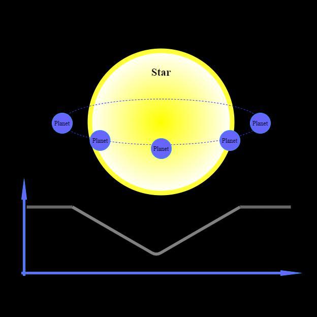
Fig -1: Transit photometry: The flux intensity of the star varies at different point of time as the planet moves around the star. The presence of periodic dips in the intensitycurvescanconfirmthepresenceofanexoplanet. information about exoplanet atmospheres and compositions,aswellastheirhoststars.Itcanalsohelpus understand how the solar system formed. In total, 5190 exoplanets have been identified as of October 2022[1]. The standard exoplanet detection techniques include direct imaging, Doppler Spectroscopy , astrometry, microlensing, and the transit method [2]. Most of the known planets have been discovered by the transit method. If we detect periodic drops in flux intensities of thestarwhenaplanetpassesinfrontofit,wecanconfirm thataplanettransitsaroundthestar.Inthispaperweuse the transit method of analysing light curves. However, analysingthefluxcurvetofindthemisaverytedioustask because vast amounts of data are produced from the observatoriesthatareoftennoisy.

International Research Journal of Engineering and Technology (IRJET) e-ISSN:2395-0056

Volume: 09 Issue: 11 | Nov 2022 www.irjet.net p-ISSN:2395-0072

Thesearchofexoplanetstookastepforwardwiththehelp of observatories such as Kepler [3], the CoRoT spacecraft [4], the Transiting Exoplanet Survey Satellite (TESS) [5], andothers[6-8].AlthoughtheKeplermissionconcludeda fewyearsagoandthedataiswell-systemisedandpublicly available, it is still far from being completely put to use. These data can provide insights that could pave the way for future discoveries in the coming decades. Usually professional teams manually inspect the light curves for possible planet candidates. They vote for each other to reach a final decision after concluding their study [9,10]. To properly and quickly determine the presence of these planetswithoutanymanualefforts,itwillbenecessaryto automatically and reliably assess the chance that individual candidates are, in fact, planets, regardless of low signal-to-noise ratios-the ratio of the expected dip of the transit to the predictable error of the observed averageofthelightintensitieswithinthetransit.

Furthermore, exoplanet classification is an example of an imbalanced binary classification problem. The issue with the data is that the available number of stars with exoplanets is far lesser than the number of stars with no exoplanets. Fortunately, the advancements in machine learning help us to automate the complex computational tasks of learning and predicting patterns in light curves within a short time. In 2016, a robotic vetting program wasdevelopedtoimitatethehumananalysisemployedby some of the planet candidate catalogs in the Kepler pipeline [11]. The Robovetter project was a decision tree meant to eliminate the false-positive ‘threshold crossing events’(TCEs)andtodeterminewhetherthereareplanets having a size similar to that of the earth present around any Sun-like stars. Likewise, in the past several other notableattemptssuchastheautovetter[12]weremadeto propound the applications of machine-learning methodologiesinspottingexoplanetsin Keplerlightcurve data.

Since the introduction of the Astronet, a deep learning model that produced great results in automatic vetting of Kepler TCEs [13] the advantages of using deep learning models for the classification of the light curves are more investigated. Despite the fact that deep learning methods are computationally expensive, since they offer better results for complex problems, many researchers attempt to shift their attention from classical machine learning methodstodeeplearningmethods.Also,asdeep learning is a dynamic field that is constantly evolving, there are possibilities of new techniques other than the conventionalmodelsthatmightprovetobemoreefficient in exoplanet detection. Also, as astronomical projects include long-term strategies and are critical in educational, environmental and economical aspects, researches should adhere to accuracy and ethics. The biased research could cynically affect the scientific

training,educationandfinancingoffutureastronomers.In exoplanetdetection weshouldnotfalsifyorleaveoutany potential exoplanet candidates and fully harness the data availablefromthemissions.Beingmotivatedbythese, we propose two deep learning models, Semi Supervised Generative Adversarial Networks (SGAN) and Auxiliary Classifier Generative Adversarial Networks (ACGAN), for the classification of exoplanets. We call these methods ExoSGAN and ExoACGAN respectively. They produce comparableandsometimesbetter classificationresultsto thetechniquessofarused.

Thepaperisorganizedintosixsections.Section2includes relevant works in this field. Section 3 contains an explanation of the methodologies utilized in this article. Section4discussesthematerialsused, datapreprocessing prior to creating our model along with the architecture used to create the models. Section 5 discusses the evaluation measures utilized and the findings obtained. The study closes with a section that summarises the findingsandfuturedirectionsinthisresearchfield.

2. RELATED WORKS

Alothashappenedintherealmofastrophysicsaswellas deep learning in the last 25 years. Many researchers are investigating the use of deep learning algorithms for exoplanetdiscovery.Oneofthewidelyusedtechniquesfor the detection of extrasolar planets include Box-fitting Least Squares(BLS)[14]. The approach is based on the box-shapeofrecurrentlightcurvesandtakesintoaccount instanceswithlowsignal-to-noiseratios.Theyusebinning to deal with the massive number of observations. They point out that an appreciable identification of a planetary transit necessitates a signal-to-noise ratio of at least 6. Cases that appear to be a good fit are then manually assessed. However, the method is exposed to the risk of false-positive detections generated by random cosmic noisepatterns.

A transit detection technique that makes use of the random forest algorithm is the signal detection using randomforestalgorithm(SIDRA)[15]. SIDRAwastrained on a total of 5000 simulated samples comprising 1000 samples from each class namely constant stars, transiting light curves, variable stars, eclipsing binaries and microlensing light curves. 20,000 total samples from thesedifferentclassesweretestedwhereasuccessratioof 91percentisachievedfortransitsand95-100percentfor eclipsing binaries, microlensing, variables and constant light curves. They recommended that SIDRA should only be used in conjunction with the BLS method for detecting transiting exoplanets since SIDRA had generated low resultsontransitinglightcurves.

In 2017, Sturrock et al [16] conducted a study on the use of the machine learning methods namely, random forest (RF), k-nearest neighbour (KNN) and Support Vector

International Research Journal of Engineering and Technology (IRJET) e-ISSN:2395-0056

Volume: 09 Issue: 11 | Nov 2022 www.irjet.net p-ISSN:2395-0072

Machine(SVM)inclassifyingcumulativeKOIdata (Kepler Objects of Interest). In terms of the fraction of observationsidentifiedasexoplanets,SVMdidnotgivethe desired prediction results. The RF model has the risk of overfitting the dataset. Inorder to reduce overfitting, measures such as StratifiedShuffleSplit, feature reduction, cross validation etc had to be done. It was found that random forest gave a cross-validated accuracy of 98 percentwhichisthebestamongtheotherthreemethods. Using Azure Container Instance and an API (application programming interface) the random forest classifier was madeaccessibletopublic.

In 2018, Shallue and Vanderburg [13] researched about identifyingexoplanetswithdeeplearning.Thisisanotable workinthefieldandisconsideredtobethestateoftheart method. They used NASA Exoplanet Archive: Autovetter Planet Candidate Catalog dataset and introduced a deep learning architecture called Astronet that utilizes convolutionalneuralnetworks(CNN).Thereare3separate input options to the network: global view, local view and both the global and local views. These input representationswerecreatedbyfoldingtheflattenedlight curvesontheTCEperiodandbinningthemtoproducea1 dimensional vector. During training they augmented the training dataset by using random horizontal reflections. They used the google-vizier system to automatically tune the hyperparameters including the number of bins, the numberoffullyconnectedlayers,numberofconvolutional layers,dropoutprobabilitiesetc.Aftermodeloptimization they used model averaging on independent copies of the model with different parameter initializations to improve the performance by not making the model depend upon different regions of input space. The best convolutional model received AUC (Area Under the Curve) of 0.988 and accuracyof0.960onthetestset.

Astronet K2, a one-dimensional CNN with maxpooling, was trained in 2019 to discover planet candidates in K2 data[19].Thisdeeplearningarchitectureisadaptedfrom the model created by Shallue and Vanderburg [13]. It resulted in a 98 percent accuracy on the test set. EPIC 246151543 b and EPIC 246078672 b were discovered as genuine exoplanets by Astronet K2. They are both in betweenthesizerangeoftheEarthandNeptune.Looking at the precision and recall of Astronet K2, if the classification threshold is set such that the model offers a recallof0.9inthetestsetofKeplerdata,theprecisionrate will only be 0.5. For Astronet K2 to estimate planetary occurrenceratesinK2datathemodelshouldbeenhanced to produce a recall of 90 percent while simultaneously maintaining a precision of 95 percent because K2 data containsmorefalsepositivesamples.

Later in 2020, 'TSfresh' library and 'lightbgm' tool was used in exoplanet detection by Malik et al[20] . An ensemble of decision trees called gradient boosted trees (GBT) and 10-fold CV (cross validation) technique were used to create a model to classify light curves into planet

candidates and false positives. Their prediction results in an AUC of 0.948, precision of 0.82 and recall of 0.96 in Kepler data. They provide comparable results to Shallue and Vanderburg [13] and also prove that their method is more efficient than the conventional BLS( box least squaresfitting).However,theperformanceofthismethod waspoorontheclassimbalancedTESSdata.

Yipetal[21]usedgenerativeadversarialnetworks(GAN) to detect planets through direct imaging technique. GAN was used to create a suitable dataset which is further trainedusingconvolutionalneuralnetworksclassifierthat can locate planets over a broad range of signal-to-noise ratios.

Mostofthestudiesrelatedtousingartificialintelligencein exoplanet detection utilize the random forest algorithm [23,24] and CNNs [25,26]. Other heuristic approaches to find extrasolar planets using stellar intensities include KNN [17] and self-organizing maps [18]. In 2021 PriyadarshiniandPuri[22]usedanensemble-CNNmodel on the Kepler light curves. Different machine learning algorithms such as Decision Tree, Logistic Regression, MLP (Multilayer Perceptron), SVM( Support Vector Machines, CNN, random forest classifier and their proposed ensemble-CNN model were implemented and comparedwitheachother.Theyusedastackedmodelthat is trained similarly as k-fold validation. The decision tree, RF,SVM,andMLPmodelswerethemetalearnersandCNN model was employed as base learner in their proposed work. The model was capable to produce an accuracy of 99.62 percent. However training ensemble models can be expensive and hard to interpret since we deal with light curves.

Furthermore, the use of semi supervised generative adversarial algorithm (SGAN) have been proved to be efficient in retrieving potential radio pulsar candidates [27].ThestudyindicatesthatSGANoutperformsstandard supervised algorithms in real world classification. The best performing model in the study gives an overall Fscore of 0.992. This model has been already incorporated into the HTRU-S Lowslat survey post-processing pipeline, andithasfoundeighteenadditionalpulsars.

Moreover, auxiliary classifier generative adversarial networks (ACGAN) have been useful in situations where imbalanceddataisavailableforstudy.Forinstance,Wang etal[28]developedaframeworkthatgivesimprovedand balanced performance for detecting cardiac arrhythmias using a data augmentation model and ACGAN. They also find that ACGAN based data augmentation framework gives better classification results while addressing imbalanceddata. Additionally,Sutedjaetal[29]suggested an ACGAN model to tackle an imbalanced classification issueoffrauddetectionindebitcardtransactiondata.The study also compares the classification performance of the ACGAN model used with that of a CNN model-having similar architecture to the ACGAN discriminator model.

International Research Journal of Engineering and Technology (IRJET) e-ISSN:2395-0056

Volume: 09 Issue: 11 | Nov 2022 www.irjet.net p-ISSN:2395-0072

They believe that because the ACGAN model produces better outcomes, it may also be used to solve unbalanced classificationissues.

These studies reveal that exoplanet detection issue has been approached using standard artificial intelligence techniques but it remains a challenge that deserves more attention. Hardly any exploration has been done that reveals the use of novel deep learning techniques in astronomy. We capitalize the usage of the irrefutably appealing efficiency of semi-supervised generative adversarial networks and auxiliary classifier generative adversarialnetworkstotackletheissue.Thesearealready proved to be useful in biomedical applications and other fields.

3. METHODS

3.1 Generative Adverserial Networks

function of GAN can be derived from the loss function of binarycrossentropy.

where y is the original data and is the reconstructed data.ThelabelsfromPdata (x)is1.D(x)andD(G(z))arethe discriminator'sprobabilities thatxisreal andG(z) isreal. Substituting them in equation (1) for real and fake samples, we get the two terms log(D(x)) and log(1D(G(z)).InordertoclassifyrealandfakesamplesDtriesto maximize the two terms. Generator’s task is to make D(G(z)) close to 1, therefore it should minimize the two terms above. Thereby, they follow a two player minmax game.The loss function of GAN can be expressed as follows,

minGmaxDV(D,G)=Ex~Pdata(x)[logD(x)]+Ez~Pz(z)log(1(D(G(z))] (2)

Erepresentsexpectation.

3.2 Semi-Supervised Generative Adversarial Networks(SGAN)

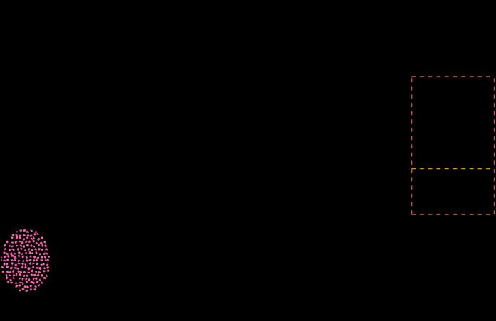
Fig -2: An overview of the GAN framework at a high level.Thegeneratorgeneratesfakesamples.Discriminator accepts false and real data as input and returns the likelihoodthattheprovidedinputisreal.

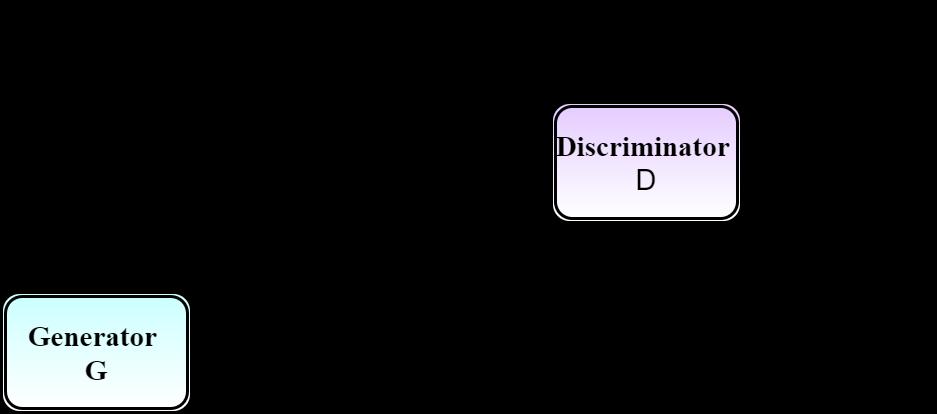
Goodfellow et al (2014) [30] introduced Generative Adversarial Networks in 2014. A generator G and a discriminator D are the two major components of this machinelearning architecture. Both of them are playing a zero-sum game in which they are competing to deceive one other. The concept of the game can be summarized roughly as follows: The generator generates images and attempts to fool the discriminator into believing that the produced images are real. Given an image, the discriminator attempts to identify whether it is real or generated. The notion is that by playing this game repeatedly, both players will improve, which implies that the generator will learn to produce realistic images and the discriminator will learn to distinguish the fake from thegenuine.

Gisagenerativemodelwhichmapsfromlatentspacez to the data space X as G(z;Ө) and tries to make the generative samples G(z) as close as possible to the real datadistributionPdata (x).Pz(z)isthenoisedistribution.D [givenbyD(x;Ө2)]discriminatesbetweentherealsamples of data (labeled 1) and the fake samples (labeled 0) generated from G and outputs D(x) ∈ (0,1). The loss

Fig -3:IllustrationofArchitectureofExoSGAN

An extension to GAN was made by Odena (2016) [31] called SGAN to learn a generative model and a classification job at the same time. Unlike the traditional GAN that uses sigmoid activation function to distinguish between real and fake samples, SGAN uses softmax function to yield N+1 outputs. These N+1 include the classes1toNandthefakeclass.Salimansetal(2016)[32] presentedastateoftheartmethodforclassificationusing SGANonMNIST,CIFAR-10andSVHNdatasetsatthattime. InourcaseSGANshouldproduceoutputs-exoplanets,non exoplanetsandfakesamples.Takingxasinput,astandard supervised classifier produces the class probabilities (stars having exoplanets and stars having no exoplanets). We achieve semi-supervised learning here by providing thegeneratedfakesamplesfrom Glabeledy=N+1tothe D and categorising them as fake samples thereby

International Research Journal of Engineering and Technology (IRJET) e-ISSN:2395-0056

Volume: 09 Issue: 11 | Nov 2022 www.irjet.net p-ISSN:2395-0072

introducing an additional dimension. Let the model predictive distribution be (Pmodel(y| x)) as in case of a standardclassifierwhereyisthelabelcorrespondingtox. Pmodel(y=N+1|x)givestheprobabilitythatxisfake.

The loss function of SGAN consists of an unsupervised andasupervisedcomponent.

L=Lunsupervised+Lsupervised (3)

The unsupervised component has two parts. Given the data being real, one minus the expectation of the model producingthe resultasfake constitutesthefirst part. The next part is the expectation of the model producing the resultasfakewhenthedataisfromG.

WecannoticethatsubstitutingD(x)=1-Pmodel(y=N+1| x)intotheLunsupervised yieldsequation2.

Lunsupervised =-Ex~Pdata(x)log[1-Pmodel(y=N+1|x)]+ Ex~Glog[Pmodel(y=N+1|x)] (4)

If the data is from any of the N classes, the supervised losscomponentisthenegativelogprobabilityofthelabel.

Lsupervised =-Ex,y~Pdata(x,y) logPmodel (y|x,y<K+1) (5)

Therefore,thelossfunction ofSGANcanbegivenas

L = -Ex,y~Pdata(x,y)[logPmodel(y|x)]Ex~G[logPmodel(y=N+1|x)] (6)

The output of the softmax does not change when a common function f(x) is subtracted from each of the classifier'soutputlogits.SoifwefixthelogitsoftheN+1th class to 0, the value doesn’t change. Finally if Z(x) = ∑ is the normalized sum of the exponentialoutputs,thediscriminatorcanbegivenas (7)

Mirza and Osindero [33] presented conditional GAN (CGAN),anenhancementtoGAN,toconditionallygenerate samples of a specific class. The noise z along with class labels c are given as input to generator of CGAN to generatefakesamplesofaspecificclass(Xfake=G(c,z)).This variation improves the stability and speed while training GAN.ThediscriminatorofCGANisfedwithclasslabelsas one of the inputs. ACGAN is a CGAN extension in which instead of inputting class labels into D, class labels are predicted. It was introduced by Odena et al [34]. The discriminator of ACGAN can be thought of as having two classification functions: one that predicts whether the input is real or false(probability P(S|X)), and another that classifies the samples into one of the classes(probability P(C|X)). LC, the log-likelihood of the correct class and LS , the log likelihood of the source make up the two parts of thelossfunctionofACGAN.

LS=E[logP(S=real|Xreal)]+E[logP(S=fake|Xfake)] (8)

LC=E[logP(C=c|Xreal)]+E[logP(C=c|Xfake)] (9)

The generator and discriminator play a minmax game on LS asincaseofnormalGAN.TheytrytomaximiseLC.In contrast to the conditional GAN, the resultant generator learns a latent space representation irrespective of the classlabel.

4. DATA SOURCES AND IMPLEMENTATION

4.1 Dataset

3.3 Auxillary

Classifier

Generative Adversarial Networks(ACGAN)

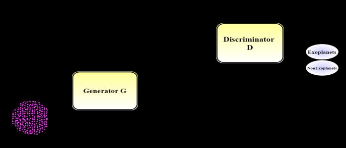
Fig -4:IllustrationofArchitectureofExoACGAN

Kepler Mission: NASAbegantheKeplermissiononMarch 7, 2009, to study stars and hunt for terrestrial planets, particularly habitable planets with liquid water. Two of Kepler's four reaction wheels malfunctioned by May 11, 2013. At least three of them should be in good shape to keepthespaceshippointedintherightdirection.Because thedamagecouldnotberepaired,theK2-"SecondLight"wasinitiated(February4,2014),whichtakesadvantageof Kepler's remaining capabilities. K2 conducted eclipticpointed ‘Campaigns’ of 80 days duration. The light intensities were recorded every 30 minutes. These stellar lightintensitiesareusedtolookfordipsinordertodetect anyprobableexoplanetstransitingthestar.Atotal of477 confirmedplanetswerefoundbyK2asofDecember2021. We use data from K2's third campaign, which began on November 12th, 2014, for this study. A few samples from othercampaignswerealsousedtoenhancethenumberof stars containing exoplanets. However, Campaign 3 accounts for nearly all of the data. Almost 16,000 stars were included in the field-of-view(FOV) of the third Campaign.Kepler’sdatawasmadepublicbyNASAviathe Mikulski Archive. We used the open-sourced data from Kaggle [35] which was created by transposing the PDCSAP-FLUX column(Pre-search Data Conditioning) of the originalFITSfile.

International Research Journal of Engineering and Technology (IRJET) e-ISSN:2395-0056

Volume: 09 Issue: 11 | Nov 2022 www.irjet.net p-ISSN:2395-0072

Train and test data: The train set includes 5087 observations,eachwith3198features.Theclasslabelsare listedinthefirstcolumn.Label2denotesstarshaving

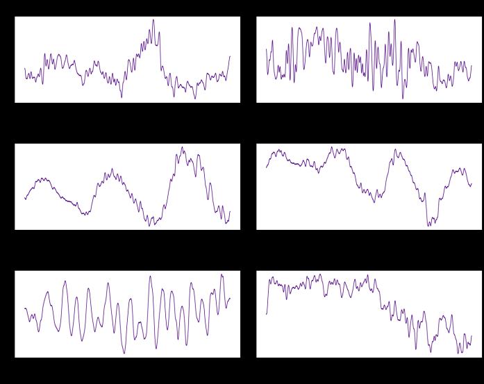
Fig -5: Plot of the light curves of a few stars from the dataset with exoplanets and without exoplanets-before preprocessing. X-axis gives the time and Y-axis shows the flux intensities. The curves are not normalized and standardized.Alsonotethepresenceofhugeoutliers.

exoplanets, whereas label 1 denotes stars without exoplanets.Thesameistrueforthetestset.Thefollowing columns2-3198showtheintensityoflightemittedbythe stars at equal time intervals. As the Campaign lasted 80 days, the flux points were taken around 36 minutes apart (3197/80). There are 545 samples in the test data, 5 of whichcontainexoplanets.Thesearetheunseendataused totestthemethod'soutcomes.Wehaverenamedtheclass labels, 1 for exoplanet-stars and 0 for nonexoplanet-stars for convenience. Figure 5 illustrates few samples from traindata.

4.2 Data Pre-processing

1. Thedatacontainsnoduplicatesandnullvaluesas ithasalreadybeende-noisedbyNASA.

2. When we take a look at the data, we notice that there are many outliers in intensity values. Since wesearchfordips,itisimportantnottoeliminate outlier clusters caused by transits that naturally belong to the target star. So we remove a tiny fraction of the upper outliers and replace them with mean of adjacent points. Later Fast Fourier Transform, followed by gaussian filter is applied to convert the raw flux from temporal to frequencydomainandsmoothenthecurve.

3. As the features are in various ranges, we should normalizethedatasuchthattherowvaluesrange between -1 and 1. We may also standardize the data by using StandardScaler to ensure the column values have a standard deviation of one. Figure 6 illustrates the light curves after the preprocessingsteps.

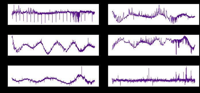
Fig -6: Plot of the light curves of a few stars with exoplanetsandwithoutexoplanets-afterpreprocessing.Xaxis shows the frequency and Y-axis plots the flux intensity. The curves are normalized and standardized as wellasconvertedintofrequencydomain.Themajorupper outliersarealsoremoved.

4.3 Model Architecture and Training : ExoSGAN

The generator G takes noise from a random normal distribution (standard deviation 0.02) in the latent space and generates fake flux curves, which are one of three inputs to D. The true dataset, which comprises the flux curveas well asitslabels,is the next inputtoD. The final setofinputscomesfromrealsamplesaswell,butthistime theyareunlabeled.

A convolutional neural network with two output layers, one withloss function binarycross entropyandtheother with sparse categorical cross entropy, makes up the discriminator network. The second output layer uses a softmax activation function to predict the stars with and without exoplanets while the first output layer uses sigmoid activation to find the realness of the data. In the generator a transpose of 1 dimensional convolutional layer followed by dense layers is used. We also use BatchNormalisation and LeakyReLu with a slope of 0.2. A tanhactivationfunctionisemployedintheoutputlayer.

Wegetabetterperformancemodelwhenweincreasethe number of labeled samples to 148 (74 positive and 74 negativesamples).Toslightlyincreasethepositivelabeled real samples we reverse the order of the flux points preservingtheshapeandaddthemtotheoriginaldataset. Now the train dataset contains 74 light curves with exoplanets and 5050 light curves with no exoplanets. Still the imbalance remains the same with ratio 1:100 exoplanetandnonexoplanetstars.

The training procedure of GAN includes holding D constantwhiletrainingGandviceversa.Weusealearning rate η=4e-6 and β1= 0.5. G is trained via D and Discriminator D is a stacked model with shared weights

International Research Journal of Engineering and Technology (IRJET) e-ISSN:2395-0056

Volume: 09 Issue: 11 | Nov 2022 www.irjet.net p-ISSN:2395-0072

wheretheresultscanbereused. Theunsupervisedmodel is stacked on top of the supervised model before the softmaxactivationfunctionwheretheformertakesoutput fromthelatter.

Figure 3 shows the SGAN model architecture used in this paper.

4.3 Model Architecture and training: ExoACGAN

In the architecture adopted here, we feed random noise and the class labels of exoplanet and non-exoplanet light curves into the generator, which subsequently produces synthetic data. The discriminator receives created flux intensity curves as well as real flux intensity curves as input. It guesses if the data is authentic or bogus and distinguishes between light curves with and without exoplanets.

The discriminator is implemented as a 1-dimensional convolutional network with input shape(3197,1). The learningrate ofDissettoη=4e-5whilethatofGisη=4e6. SimilartoExo-SGAN,Dhastwooutputlayerswherethe first predicts real/fake class and the second gives the probability of the stars having exoplanets. The generator model takes in latent space with 100 dimensions and the single integer class labels. The latent vector is given to a dense layer and later reshaped. We use an embedding layerinGtofeaturemaptheclasslabelswithadimension of 10 (arbitrary). This can then be interpreted by a dense layer. Afterwards, the tensors formed by noise and class labels are concatenated producing an additional channel andsentthrougha1-dimensionalconvolutionaltranspose layer,whichisflattenedand then passedthrough3dense layers later to finally produce curves of 3197 flux points. Also, LeakyRelu and Batch normalisation are used to provideregularization.Theoutputlayerisdesignedwitha hyperbolictangentactivationfunction.ACGAN also uses a compositemodellikeSGANwherethegeneratoristrained via the discriminator. Figure 4 shows the SGAN model architectureusedinthispaper.

5. EVALUATION

5.1 Metrics used for evaluation

1. Confusion Matrix: The summarization of the classification performed by Exo-SGAN and ExoACGAN can be given by a confusion matrix. It provides information not only on the faults produced, but also on the sorts of errors made. For binary classification, it is a 2x2 matrix of actual and predicted positive and negative classificationsasgiveninTable1: where,

TP : True positive (A star with exoplanet predictedasastarwithexoplanet)

FP: False positive (A star without exoplanet predictedasastarwithexoplanet)

FN: False negative (A star without exoplanet predictedasstarwithexoplamet)

TN: True negative (A star without exoplanet predictedasastarwithoutexoplanet)

Table -1: Confusionmatrixforexoplanetclassfication

2. Accuracy: When evaluating a model for classification issues, accuracy is frequently used. As the name implies, accuracy is the number of right predictions divided by the total number of predictions. An accuracy of 1.00 means that all of thesampleswereproperlycategorized. However, in this situation, as the data we have is very imbalanced, accuracy alone cannot be used to evaluate the performance of the models since an 99 accuracy of 0.99 might also suggest that all of thesamplesareplacedintothemajorityclass.

3. Precision: Precision seeks to address the issue of how many positive identifications were truly correct. A precision of 1 indicates that the model produced no FP. To find precision we use the formula

Precision is the ratio between the true positives to the total of true positivesandfalsepositives.

4. Recall: The proportion of positive samples recovered is referred to as recall. It is a useful metric when we need to accurately categorise all of the positive samples. Sensitivity is another termforrecall.

International Research Journal of Engineering and Technology (IRJET)

e-ISSN:2395-0056

Volume: 09 Issue: 11 | Nov 2022 www.irjet.net p-ISSN:2395-0072

Table -3: ConfusionmatrixofExo-ACGANmodelon training dataset

5. Specificity: Specificity is found by dividing the true negatives by the total number of actual negative samples. Specificity answers the question of how many stars with no exoplanets didthemodelaccuratelypredict.

6. F-betascore:Theharmonicmeanofprecisionand recall is used to get the F-score. F-beta is an abstraction oftheF-scorein whichthe balanceof precision and recall in the computation of the harmonicmeanisregulatedbyacoefficientcalled β. In the computation of the score, a beta value greater than 1.0, such as 2.0, provides more weighttorecallandlessweighttoprecision.

Fβ F-2Scorecanbeobtainedbysubstitutingβ=2.

F2 =

5.2 Results and Discussion

The ExoSGAN and ExoACGAN models produce encouraging results in the classification of exoplanets. It should be noted that to the best of our knowledge semisupervised generative adversarial networks and auxiliary classifier generative adversarial networks have not yet been used for the classification of exoplanet stars. Based on our findings, we believe that these approaches are extremely promising for detecting exoplanets from light curves.

Table -2: ConfusionmatrixofExo-SGANmodelon training dataset

Predicted: without exoplanet

Predicted: with exoplanet

Total

Actual:without exoplanet 5032 18 5050

Actual:with exoplanet 0 74 74 Total 5032 92 5124

Predicted: without exoplanet

Predicted: with exoplanet

Total Actual:without exoplanet 5041 9 5050 Actual:with exoplanet 0 74 74 Total 5041 83 5124

Table -4: ConfusionmatrixofExo-SGANandExo-ACGAN modelon testing dataset

Predicted: without exoplanet

Predicted: with exoplanet

Total Actual:without exoplanet 565 0 565 Actual:with exoplanet 0 5 5 Total 565 5 190

Table -5: ResultsoftheperformanceofExo-SGANmodel ontrainandtestdata

Exo-SGAN Training Testing

Accuracy 0996 100 Precision 0.804 1.00 Recall 100 100 Specificity 0996 100 F-Score 0.954 1.00

Table -6: ResultsoftheperformanceofExo-ACGANmodel ontrainandtestdata

Exo-SGAN Training Testing

Accuracy 0998 100 Precision 0892 100 Recall 1.00 1.00 Specificity 0998 100 F-Score 0976 100

International Research Journal of Engineering and Technology (IRJET) e-ISSN:2395-0056

Volume: 09 Issue: 11 | Nov 2022 www.irjet.net p-ISSN:2395-0072

We argue that, among the assessment criteria described above, recall is the most important since we should not overlookanystarswithexoplanets.Asaresult,wetrained our models to provide the highest possible recall. Maximum recall is at the expense of precision. A model withhighrecall mayhavelowprecision.Thisisknown as the precision-recall trade-off. In our case, having a few starswithout exoplanetslabelledasstarswith exoplanets can be compromised if we can properly categorise each starwithexoplanets.Itisimportanttorememberthatthe data is extremely biased with a majority of non exoplanet candidate stars. Therefore as mentioned earlier, accuracy cannotbeconsideredasapropermetricforevaluation.As we place greater emphasis on recall, we increase the weightofrecallintheF-scoreandsetthebetavalueto2.

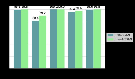
The models, both ExoSGAN and ExoACGAN, output probabilities of a star containing exoplanet. The default threshold for such a classification task is often set at 0.5. Sincewedealwithimbalanceddataandaimtotakeoutall the lighcurves containing the transit, we should optimize the threshold. We choose our threshold to be 0.81 for the semi-supervised classification model and 0.77 for the auxiliaryclassifiergenerativeadversarialnetwork.Bothof these models give us a perfect recall of 1.00 on the train andtestsetforthechosenthreshold.Wegetaprecisionof 0.802 from Exo-SGAN and 0.892 from Exo-ACGAN on the train data. While training, Exo-ACGAN results in an accuracy of 99.8 whereas Exo-SGAN gives an accuracy of 99.6. When we test our models on unseen data both ExoACGAN and Exo-SGAN give a perfect accuracy of 100 percent.Allthe565non-exoplanetstarsand10exoplanet starsinthetestsetare

Chart -2:Acomparisonoftheoutcomesofeachofthe Exo-SGANandExo-ACGANassessmentmetricsusingtest data

classified correctly. Therefore, the precision, recall, specificity, and f-score turns out to be 1.00 for both ExoSGAN and Exo-ACGAN on test data as shown in Table 5 and 6. On the train samples, out of 5050 non-exoplanet stars only 8 have been misclassified by Exo-ACGAN, and only 18 have been misclassified by Exo-SGAN. The confusion matrix in Table 2, 3 and 4 tabulates the classificationresultsofourexperiments.

WhenwecompareExo-SGANandExo-ACGAN,wecanfind that ACGAN marginally surpasses Exo-SGAN. Both have a recallofone,butthelatterhasagainof0.2,0.09,and0.09 inaccuracy,precision,andspecificitywhiletraining.

It can be speculated that during the training and testing procedure of Exo-ACGAN, the adversarial training technique assisted in reducing the impact of the imbalanceddataset.Asaresult,theprejudicetowardsthe majority class is reduced. The discriminator model is taught to learn patterns from both actual and generated datainanadversarialmanner.Asaconsequence,inorder to generalize the patterns from the training dataset, the discriminator model learnt a greater number of richer patterns.

6. CONCLUSIONS AND FUTURE WORKS

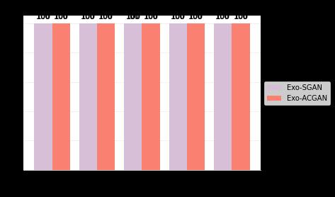
Chart -1:Acomparisonoftheoutcomesofeachofthe Exo-SGANandExo-ACGANassessmentmetricsusingtrain data

In this paper, we utilise the Semi-Supervised Generative Adversarial framework and Auxilary Classifier Generative Adversarialframeworktodetectexoplanetsusingtheflux curves of stars. The performance of both methods is noteworthy since both of them properly detect all lightcurves with transit. Exo-SGAN and Exo-ACGAN both has a recall rate of 100. The capacity to use unlabeled candidates to get better outcomes is the key advantage of our proposed network Exo-SGAN. We anticipate that, as the number of exoplanet candidates increase and maintaining a big labelled dataset becomes more difficult, this method will become even more beneficial for future exoplanet detection. Even though the data is extremely unbalanced, Exo-ACGAN and Exo-SGAN are able to

International Research Journal of Engineering and Technology (IRJET) e-ISSN:2395-0056

Volume: 09 Issue: 11 | Nov 2022 www.irjet.net p-ISSN:2395-0072

produce better results even without the use of any upsamplingapproacheslikeSMOTE.

As for the next steps, these architectures can be tried out on the raw lightcurves from the Kepler mission, provided Graphical Processing Units(GPU) and hardware of great performance since a large amount of data must be handled. The hyperparameters can also be tuned to give better performance. Additionally, experimenting with various data-preprocessing approaches for eliminating outliers may improve the performance. One method to attempt in order to solve the class imbalance issue is to optimize the loss function to produce data only from the minorityclasswhiletraining[36].Thiscanbringabalance between the samples of both classes. Yet another techniquetoimprovetheclassificationaccuracyistheuse of Bad GAN [37] in which the generator’s goal is more focused to produce data that complements the discriminator’sdata.

However, our models can provide a very reliable system forfindingall thetruepositivesin ourdata atthecurrent stage. It is hoped that these deep learning approaches wouldpavethewayforanewerainthefieldofexoplanet hunting.

REFERENCES

[1] https://exoplanetarchive.ipac.caltech.edu/docs/count s_detail.html

[2] Fischer, D.A., Howard, A.W., Laughlin, G.P., Macintosh, B., Mahadevan, S., Sahlmann, J., Yee, J.C.: Exoplanet detection techniques. Protostars and Planets VI (2014).https://muse.jhu.edu/chapter/1386909

[3] Borucki, W.J.: KEPLER Mission: development and overview. Reports on Progress in Physics 79(3), 036901 (2016). https://iopscience.iop.org/article/10.1088/00344885/79/3/036901

[4] Grziwa, S., P¨atzold, M., Carone, L.: The needle in the haystack:searchingfortransitingextrasolarplanetsin CoRoT stellar light curves. Monthly Notices of the Royal Astronomical Society 420(2), 1045–1052 (2012)

[5] Ricker, et.al Journal of Astronomical Telescopes, Instruments, and Systems, Vol. 1, Issue 1, 014003 (October 2014). https://doi.org/10.1117/1.JATIS.1.1.014003

[6] Collier Cameron, A., Pollacco, D., Street, R.A., Lister, T.A., West, R.G., Wilson, D.M., Pont, F., Christian, D.J., Clarkson, W.I., Enoch, B., Evans, A., Fitzsimmons, A., Haswell,C.A.,Hellier,C.,Hodgkin,S.T.,Horne,K.,Irwin, J., Kane, S.R., Keenan, F.P., Norton, A.J., Parley, N.R.,

Osborne, J., Ryans, R., Skillen, I., Wheatley, P.J.: A fast hybrid algorithm for exoplanetary transit searches. Monthly Notices of the Royal Astronomical Society 373(2), 799–810 (2006) https://doi.org/10.1111/j.1365-2966.2006.11074.x

[7] Hartman,J.D.,Bakos,G.A.,Torres,G.:Blendanalysisof hatnet transit ´ candidates. EPJ Web of Conferences 11,02002(2011).

[8] Maciejewski, G., Fern´andez, M., Aceituno, F. J., Ohlert, J., Puchalski, D., Dimitrov, D., Seeliger, M., Kitze, M., Raetz, St., Errmann, R., Gilbert, H., Pannicke, A., Schmidt, J.-G., Neuh¨auser, R.: No variations in transit timesforqatar-1b.A&A577,109(2015).

[9] Crossfield, I.J.M., Guerrero, N., David, T., Quinn, S.N., Feinstein, A.D., Huang, C., Yu, L., Collins, K.A., Fulton, B.J., Benneke, B., Peterson, M., Bieryla, A., Schlieder, J.E.,Kosiarek,M.R.,Bristow, M.,Newton,E.,Bedell,M., Latham, D.W., Christiansen, J.L., Esquerdo, G.A., Berlind, P., Calkins, M.L., Shporer, A., Burt, J., Ballard, S., Rodriguez, J.E., Mehrle, N., Dressing, C.D., Livingston, J.H., Petigura, E.A., Seager, S., Dittmann, J., Berardo, D., Sha, L., Essack, Z., Zhan, Z., Owens, M., Kain, I., Isaacson, H., Ciardi, D.R., Gonzales, E.J., Howard,A.W.,de,M.C.J.V.:VizieROnlineDataCatalog: Variablestarsandcand.planetsfromK2(Crossfield+, 2018).VizieROnlineDataCatalog,239–5(2018)

[10] Yu, L., Vanderburg, A., Huang, C., Shallue, C.J., Crossfield, I.J.M., Gaudi, B.S., Daylan, T., Dattilo, A., Armstrong,D.J.,Ricker,G.R.,Vanderspek,R.K.,Latham, D.W., Seager, S., Dittmann, J., Doty, J.P., Glidden, A., Quinn, S.N.: VizieR Online Data Catalog: Automated triage and vetting of TESS candidates (Yu+, 2019). VizieROnlineDataCatalog,158–25(2019)

[11] JeffreyL.Coughlin et al 2016 ApJS 22412

[12] SeanD.McCauliff et al 2015 ApJ 8066

[13] Christopher J. Shallue and Andrew Vanderburg 2018 AJ 15594

[14] A box-fitting algorithm in the search for periodic transits G. Kovács, S. Zucker, T. Mazeh A&A 391 (1) 369-377(2002)DOI:10.1051/0004-6361:20020802

[15] D. Mislis, E. Bachelet, K. A. Alsubai, D. M. Bramich, N. Parley,SIDRA:ablindalgorithmforsignaldetectionin photometric surveys, Monthly Notices of the Royal Astronomical Society, Volume455,Issue 1,01January 2016, Pages 626–633, https://doi.org/10.1093/mnras/stv2333

International Research Journal of Engineering and Technology (IRJET) e-ISSN:2395-0056

Volume: 09 Issue: 11 | Nov 2022 www.irjet.net p-ISSN:2395-0072

[16] Sturrock, G.C., Manry, B., Rafiqi, S.: Machine learning pipelineforexoplanetclassification.SMUDataScience Review2(1)(2018)

[17] SusanE.Thompson et al 2015 ApJ 81246

[18] D. J. Armstrong, D. Pollacco, A. Santerne, Transit shapes and self-organizing maps as a tool for ranking planetary candidates: application to Kepler and K2, Monthly Notices of the Royal Astronomical Society, Volume 465, Issue 3, March 2017, Pages 2634–2642, https://doi.org/10.1093/mnras/stw2881

[19] AnneDattilo et al 2019 AJ 157169

[20] Abhishek Malik, Benjamin P Moster, Christian Obermeier, Exoplanet detection using machine learning, Monthly Notices of the Royal Astronomical Society, Volume 513, Issue 4, July 2022, Pages 5505–5516,https://doi.org/10.1093/mnras/stab3692

[21] Yip, K.H., Nikolaou, N., Coronica, P., Tsiaras, A., Edwards, B., Changeat, Q., Morvan, M., Biller, B., Hinkley, S., Salmond, J., Archer, M., Sumption, P., Choquet, E., Soummer, R., Pueyo, L., Waldmann, I.P.: Pushing the limits of exoplanet discovery via direct imaging with deep learning. In: Brefeld, U., Fromont, E., Hotho, A., Knobbe, A., Maathuis, M., Robardet, C. (eds.) Machine Learning and Knowledge Discovery in Databases,pp.322–338.Springer,Cham(2020)

[22] Priyadarshini, I., Puri, V. A convolutional neural network (CNN) based ensemble model for exoplanet detection. Earth Sci Inform 14, 735–747 (2021). https://doi.org/10.1007/s12145-021-00579-5

[23] GabrielA.Caceres et al 2019 AJ 15858

[24] N Schanche, A Collier Cameron, G Hébrard, L Nielsen, A H M J Triaud, J M Almenara, K A Alsubai, D R Anderson, D J Armstrong, S C C Barros, F Bouchy, P Boumis,DJABrown,FFaedi,KHay,LHebb,FKiefer, L Mancini, P F L Maxted, E Palle, D L Pollacco, D Queloz, B Smalley, S Udry, R West, P J Wheatley, Machine-learning approaches to exoplanet transit detection and candidate validation in wide-field ground-based surveys, Monthly Notices of the Royal Astronomical Society, Volume 483, Issue 4, March 2019, Pages 5534–5547, https://doi.org/10.1093/mnras/sty3146

[25] MeganAnsdell et al 2018 ApJL 869L7

[26] Alexander Chaushev, Liam Raynard, Michael R Goad, Philipp Eigmüller, David J Armstrong, Joshua T Briegal,MatthewRBurleigh,SarahLCasewell,Samuel Gill, James S Jenkins, Louise D Nielsen, Christopher A

Watson, Richard G West, Peter J Wheatley, Stéphane Udry, Jose I Vines, Classifying exoplanet candidates withconvolutionalneuralnetworks:applicationtothe NextGenerationTransitSurvey, Monthly Notices of the Royal Astronomical Society, Volume 488, Issue 4, October 2019, Pages 5232–5250, https://doi.org/10.1093/mnras/stz2058

[27] Vishnu Balakrishnan, David Champion, Ewan Barr, MichaelKramer,RahulSengar,MatthewBailes,Pulsar candidate identification using semi-supervised generative adversarial networks, Monthly Notices of the Royal Astronomical Society, Volume 505, Issue 1, July 2021, Pages 1180–1194, https://doi.org/10.1093/mnras/stab1308

[28] P.Wang,B.Hou,S.ShaoandR.Yan,"ECGArrhythmias Detection Using Auxiliary Classifier Generative Adversarial Network and Residual Network," in IEEE Access, vol. 7, pp. 100910-100922, 2019, doi: 10.1109/ACCESS.2019.2930882.

[29] Sutedja, I., Heryadi, Y., Wulandhari, L.A., Abbas, B.: Imbalanced data classification using auxiliary classifier generative adversarial networks. InternationalJournalofAdvancedTrendsinComputer ScienceandEngineering9(2)(2020)

[30] Goodfellow, I.J., Pouget-Abadie, J., Mirza, M., Xu, B., Warde-Farley, D., Ozair, S., Courville, A., Bengio, Y.: GenerativeAdversarialNetworks(2014)

[31] Odena, A.: Semi-Supervised Learning with Generative AdversarialNetworks(2016)

[32] Salimans, T., Goodfellow, I., Zaremba, W., Cheung, V., Radford, A., Chen, X.: Improved Techniques for TrainingGANs(2016)

[33] Mirza, M., Osindero, S.: Conditional Generative AdversarialNets(2014)

[34] Odena, A., Olah, C., Shlens, J.: Conditional Image SynthesisWithAuxiliaryClassifierGANs(2017)

[35] https://www.kaggle.com/datasets/keplersmachines/ kepler-labelled-time-series-data

[36] T.Zhou,W.Liu,C.ZhouandL.Chen,"GAN-basedsemisupervised for imbalanced data classification," 2018 4th International Conference on Information Management (ICIM), 2018, pp. 17-21, doi: 10.1109/INFOMAN.2018.8392662.

[37] Dai, Z., Yang, Z., Yang, F., Cohen, W.W., Salakhutdinov, R.:GoodSemisupervisedLearningthatRequiresaBad GAN(2017)