IRJET- One and Two-Dimensional Contaminant Transport Modelling through Unconfined Aquifer

International Research Journal of Engineering and Technology (IRJET)

e-ISSN: 2395-0056

Volume: 08 Issue: 07 | July 2021

p-ISSN: 2395-0072

www.irjet.net

One and Two-dimensional Contaminant Transport Modelling through Unconfined Aquifer Mohammad Danish Assistant Lecturer, Dept. of Civil Engineering, Oxford College of Engineering and Mgt, Nepal, Former Student, Dept. of Civil Engineering, National Institute of Technology, Meghalaya, India ---------------------------------------------------------------------***----------------------------------------------------------------------

Abstract –In this study, an effort is made to develop a finite

contaminant plume, advection-dispersion, degradation, discretized domain

irrigation water, artificial recharge, soluble rock materials, fertilizers etc. Accidental breaking of sewers and percolation from the septic tank may also increase the pollution. When radioactive waste is deeply buried, there is a likelihood of groundwater getting contaminated (Gurganus, 1993).

There is a large amount of published material in the field of contaminant transport as-Guymon et al. (1970) and Nalluswami et al. (1972) used the finite element method (FEM) based on the variational principle for the solution of the dispersion problem in a rectilinear flow field. This method was found to be applicable to dispersion dominant transport only. Smith et al. (1973) compared the variational approach with the Galerkin method and concluding final more adaptable.

1.INTRODUCTION

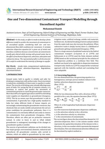
1.1 Governing Equations

difference model to predict the movement of contaminant in an unconfined aquifer, considering both one- and twodimensional flow field conditions for movement. It includes advection dispersion equation for a given set of initial and boundary conditions because concentration of contaminants usually gets altered while moving with ground water due to the effect of mechanical dispersion, advection, adsorption and radioactive decay. The represented profile in all direction for 2D is useful to understand the intensity of damage to aquifer.

Key Words: steady state, computational sophistication,

For one-dimensional flow, the governing equation in a homogeneous, isotropic porous medium reduces to the familiar advection-dispersion equation (Bear 1972):

Ground water, held in aquifer is reliable and safer for drinking in comparison with surface water. Due to increment in industries, availability of clean water in aquifers is under threat. The scarcity of drinking water already affecting many parts of India. For saving the life of common citizens, it is necessary to control and predict the movement of contaminant particles to reach the ground water resources.

More than 60% of irrigated agriculture and 85% of drinking water supplies are dependent on groundwater (Gurganus, 1993). This by no means says that groundwater is safe to contamination. It generally has a high-quality standard in India but today different kinds of human impacts are increasingly contaminating the groundwater resources. Any chemicals that are easily soluble and penetrate the soil are prime candidates for groundwater pollutants. Once it is contaminated, it is extremely difficult and costly to remove the contaminants from groundwater (Gurganus, 1993).

Therefore, efforts are often put on protective measures instead. In order to know if, and to what extent groundwater is endangered, knowledge of the changes in groundwater quality is needed.

The sources of groundwater pollution can be divided into four major groups: environmental, domestic, industrial and agricultural. All groundwater contains salts carried in solution, which are added to groundwater by rain water,

© 2021, IRJET

|

Impact Factor value: 7.529

(1.1) While for two-dimensional flow with a direction of flow parallel to the x-axis, the equation becomes (Bear 1972): (1.2) Where Dx is the longitudinal hydrodynamic dispersion coefficient.

Dy is the transverse hydrodynamic dispersion coefficient. vx is the advection velocity in the x-direction. vy is the advection velocity in y-direction.

C is the concentration of contaminants.

The current figure shows the discretized flow domain for 1-D advection-dispersion. Here i is the column number which represents the spatial discretization of the domain in the xdirection, j is the row number which represents the temporal discretization. Now one-dimensional advection-diffusion can be discretized by explicit method as –

|

ISO 9001:2008 Certified Journal

|

Page 4232

International Research Journal of Engineering and Technology (IRJET)

e-ISSN: 2395-0056

Volume: 08 Issue: 07 | July 2021

p-ISSN: 2395-0072

www.irjet.net

(1.3) (1.9) (1.4)

(1.10)

(1.5)

(1.11) Putting all above expressions in equation (1.2)-

(1.12) For computational sophistication, the flow domain is discretized in Nx+1 and Ny+1 grid points, each of length and ;

2.1 One-dimensional model

Fig. 1.1. Space and Time discretization for onedimensional finite difference formulation

To illustrate the capabilities of the model to predict the effects of advection-dispersion of contaminant transport, here a finite difference model is applied to contaminant transport problem in a saturated unconfined aquifer of finite length with constant velocity and dispersion field. It demonstrate the effect of time, advection velocity and dispersion. Flow dynamics is explained in current graphs.

Putting Eqs. (1.3), (1.4) and (1.5) in Eq. (1.1), we get

(1.6)

Fig. 2.1. Variation of contaminant with respect to distance for two different time duration when the parameters of Eq. (1.6) are given as L = 2 m, m2/day, Dt = 0.0005 day, Dx = 0.05 m, (a) day.

T = 0.5 day and (b)

Fig. 1.2. Space and time discretization for two-dimensional finite difference formulation (1.7)

(1.8)

© 2021, IRJET

|

Impact Factor value: 7.529

|

ISO 9001:2008 Certified Journal

|

Page 4233

International Research Journal of Engineering and Technology (IRJET)

e-ISSN: 2395-0056

Volume: 08 Issue: 07 | July 2021

p-ISSN: 2395-0072

www.irjet.net

(ii) As advection velocity increases from 1 m/day to 1.5 m/day, concentration of contaminant dominated till 0.6 m, plume again shifted in direction of flow beyond 2 m. It shows as velocity increases, plume shifted from one position to other position at larger scale at the same instant of time. As explained in fig. (2.2), when contaminant plume moves it disperses, present graphs show that when advection velocity increases, contaminant plume disperses at faster rate and the contaminant spreads till farther location from the source. (iii) As dispersion increases from 0.12 m2/day to 0.5 m2/day, concentration of contaminant changes with increase in dispersion at the same instant of time, it affects the spreading of contaminant plume at large scale in longitudinal directions as compare to advection velocity and time. As Fig. 2.3 (b) shows at steady state, plume is shifting from its position uniformly in forward and backward direction. If there is no dispersion, all of the contaminant will travel at same advection velocity. As dispersion increases, some contaminant travels faster and some slower. There are differences of velocity between particles, which causes spreading at larger scale. It shows, contaminant transport is affected more by dispersion as compare to advection.

Fig. 2.2. Variation of contaminant with respect to distance for two different advection velocities, when the parameters of Eq. (1.6) are given as m, m2/day, Dt = 0.0005 day, and (b) Dx = 0.05 m, (a)

3.1 Two-dimensional model Now the idea of one-dimensional modeling is extended to model the two-dimensional advection-dispersion phenomenon in an unconfined saturated aquifer. A rectangular domain of length L along x-axis and width of B along y-axis is taken for the present study. The origin of the flow domain is taken at O, which can be seen in Fig. 2.2. The dispersion and velocity field along x and y-directions are taken as Fig. 2.3. Variation of contaminant with respect to the distance for two different dispersion coefficients, when the parameters of Eq. (1.6) are given as L = 2 m,

Dx = 0.05 m, (a)

m2/day (b)

m2/day.

Impact Factor value: 7.529

respectively. The present study

Case 1: Constant velocity field along x and y-direction with different Dirichlet conditions along four faces.

In this study, a constant velocity field is taken along both the directions, whereas the boundaries along are taken as x  0, x  L, y  0, and yB

(i) As the time of simulation increases from 0.5 day to 2-day, contaminant plume in direction of flow shifted from 1.2 m to 2 m. It is observed, as time progresses the contaminant plume shifted from one place to another place. As contaminant moves it disperses, fig. (2.1) shows that the concentration decreases when it moves far away from the source of contaminant. This is the main reason; concentration of contaminant is different at different locations in the aquifer at different time.

|

and

deals with the different variations of velocity field and boundary conditions corresponding to flow diagram Fig. 2.2.

2.2 One-D model’s results and discussion

© 2021, IRJET

Dy ,

C 2 , C 4 , C 3 and C1

respectively. The mathematical

expressions for the same are given by Eqs. (2.2), (2.3), (2.4) and (2.5) respectively. An explicit finite difference methodology is used to obtain the solution of Eq. (1.2) subjected to these boundary conditions. The initial condition of the flow domain is taken as zero. Thus (2.1) C x, y, 0 = 0

(

|

)

ISO 9001:2008 Certified Journal

|

Page 4234

International Research Journal of Engineering and Technology (IRJET)

e-ISSN: 2395-0056

Volume: 08 Issue: 07 | July 2021

p-ISSN: 2395-0072

www.irjet.net

Concentration of contaminants at the entire boundary is given by

C x,0, t   C3 C x, B, t   C1 C 0, y, t   C2 C L, y, t   C4

Case 2: Different velocity field along x and y-direction with different linearly varying Dirichlet conditions along four faces.

(2.2)

This study deals with more general boundary conditions imposition as compared to case 1. The concentrations at the extreme edges of the flow domain are taken as C1 , C2 , C 3

(2.3) (2.4)

(2.5) Fig. 2.4. illustrates the variation of contaminants concentration with respect to the distance for two different time duration when the parameters of Eq. (1.12) are given as

and C 4 . However, the distributions of concentrations along any edge line are taken as linear.

For the boundary y  0, the variation of concentration is

v x  1 m/day, v y  1 m/day, x  0.05 m, y  0.05 m, t  0.5 sec, (a) T  250 sec, (b)

concentration

from

C2 to C 3 varying linearly, which can be observed from

Eq. (2.7) and for boundary y  B the variation of

L  1 m, B  1 m, Dx  2 m 2 /day, D y  2 m 2 /day,

C1 to C4 linearly, observed from Eq. (2.8).

Similarly, for boundary x = 0, the variation of concentration is from C2 to C1 varying linearly which is given by Eq. (2.9) and for boundary x = L, the variation of concentration is from C3 to C4 which is expressed by Eq. (2.10). The initial

T  4000 sec.

condition for the above-mention problem is taken as (2.6) C x, y,0  0



1



Concentration(C/C1)

0.8

Concentration of contaminants at all the boundaries are given by

0.6

0.4

0.2

0 1 0.8

1 0.6

0.8 0.6

0.4

(2.7)

æL-xö æxö C ( x, B, t ) = C1 ç ÷ + C4 ç ÷ è L ø èLø

(2.8)

æB- yö æyö C ( 0, y, t ) = C2 ç ÷ + C1 ç ÷ è B ø èBø

(2.9)

æ B- yö æyö C ( L, y, t ) = C3 ç ÷ + C4 ç ÷ è B ø è Bø

(2.10)

0.4

0.2

0.2

Distance(Y)

0

Distance(X)

0

Fig.2.4. (a) variation of contaminants concentration at T=250 sec.

1

Fig. 2.5. illustrates the variation of contaminants concentration with respect to the distance for two different time duration when the parameters of Eq. (1.12) are given as

0.9 Concentration(C/C1)

 Lx x C x,0, t   C2    C3    L  L

0.8 0.7

L  1 m, B  1 m, Dx  2.7 m 2 /day,

0.6

v x  2 m/day, x  0.05 m,

0.5 0.4 0.3 0.2 1

(b) 0.8

t  0.5 sec, (a) (c)

1 0.6

0.8 0.6

0.4 0.4

0.2

0.2

Distance(Y)

0

0

Distance(X)

Fig.2.4. (b) variation of contaminants concentration at T=4000 sec.

© 2021, IRJET

|

Impact Factor value: 7.529

|

ISO 9001:2008 Certified Journal

|

Page 4235

International Research Journal of Engineering and Technology (IRJET)

e-ISSN: 2395-0056

Volume: 08 Issue: 07 | July 2021

p-ISSN: 2395-0072

www.irjet.net

Case 3: Varying velocity field along x and y-direction with different Dirichlet conditions along four faces.

The concentrations at the extreme edges are distributed 1

uniformly in the flow domain. Are taken as Concentration(C/C1)

0.8

C1 , C2 , C 3 and

C 4 respectively. For the boundary y = 0 , concentration is

0.6

C3 , which can be observed from Eq. (2.12). Similarly for the

0.4

boundary

0.2

y = B,

concentration is

C1 ,

observed by Eq.

x = 0 , concentration is C2 , which can be observed by Eq. (2.14). Similarly for boundary x = L , concentration is C4 , observed by Eq. (2.15).

(2.13). For boundary

0 1 0.8

1 0.6

0.8 0.6

0.4 0.4

0.2

0.2

Distance(Y)

0

Distance(X)

0

Fig.2.5. (a) variation of contaminants concentration at T=250 sec

The initial condition for the above-mention problem is taken as

C x, y,0  0

(2.11)

Concentration of contaminants at all the boundary is given by following equations –

1

Concentration(C/C1)

0.8

C ( x, 0, t ) = C3

(2.12)

C ( x, B, t ) = C1

(2.13)

C ( 0, y, t ) = C2

(2.14)

C L, y, t   C4

(2.15)

0.6

0.4

0.2

0 1 0.8

1 0.6

0.8 0.6

0.4 0.4

0.2

0.2

Distance(Y)

0

Distance(X)

0

Fig. 2.6. illustrates the variation of contaminants concentration with respect to the distance for two different time duration when the parameters of Eq. (1.12) are given as

Fig.2.5. (b) variation of contaminants concentration at T=500 sec.

Dx  2 m 2 /day, 1

v x  (1  x)(1  y) ,

Concentration(C/C1)

0.9 0.8 0.7 0.6 0.5 0.4

(a)

0.3

(b)

0.2 1 0.8

1 0.6

0.8 0.6

0.4 0.4

0.2

0.2

Distance(Y)

0

0

Ditance(X)

Fig.2.5. (c) variation of contaminants concentration at T=5000 sec.

© 2021, IRJET

|

Impact Factor value: 7.529

|

ISO 9001:2008 Certified Journal

|

Page 4236

International Research Journal of Engineering and Technology (IRJET)

e-ISSN: 2395-0056

Volume: 08 Issue: 07 | July 2021

p-ISSN: 2395-0072

www.irjet.net

(ii) Figure 2.4. (b) shows the steady state of contaminants as the time passes beyond 4000 sec, contaminant will not spread more than the present concentration. Here it is observed that for two-dimensional domain also as time progresses dispersion of contaminant increases to full extent.

1

Concentration(C/C1)

0.8

(iii) Fig. 2.5. (a) clearly shows concentration of contaminants is varying linearly at all boundaries. Here advection velocity is not same in both the direction, so contaminant plume shifts from one place to other at different rate in both directions. As the distance is increasing, the contaminant concentration decreasing from all its initial values. Here also, it is observed that when the values of x and y approaches beyond 0.2 m then concentration of contaminant is minimum in this region.

0.6

0.4

0.2

0 1.5 1.5

1 1 0.5

0.5

Distance(Y)

0

0

Distance(X)

(iv) Fig. 2.5. (b) shows when the contaminant concentration increased beyond 0.4 m distance in x and y direction, region of minimum concentration starts beyond this distance. This region is smaller as compare to Fig. 2.5. (a) due to progress in time which causes more dispersion. As previous case discusses when time progresses dispersion increases due to the movement of contaminants by advection velocity.

Fig. 2.6. (a) variation of contaminants concentration at T=240 sec.

(v) Fig. 2.5. (c) shows the steady state condition where the contaminants disperse to its maximum extent for the given parameters. Beyond this time, the concentration of the contaminates will attain its peak value throughout domain; the system has reached to its saturation which can be observed from Fig.2.5. (c).

1

Concentration(C/C1)

0.9 0.8 0.7 0.6 0.5 0.4

(vi) For this case also Fig. 2.6. (a) clearly shows that maximum contamination occurs first somewhere close to corner of contamination. Here advection velocity is changing according to the position of x and y in both directions, so contaminant plume is shifting from one place to other place at different rate at different position in the region. It is observed that when the values of x and y approaches beyond 0.1 m then concentration of contaminant is minimum in this region. Here this region is larger than previous all cases. Fig. 2.6. (b) shows the steady state condition at 4000 sec for given parameters.

0.3 0.2 1.5 1.5

1 1 0.5

0.5

Distance(Y)

0

0

Ditance(X)

Fig. 2.6. (b) variation of contaminants concentration at T=4000 sec.

3.2 Two-dimensional model results (i) Fig. 2.4. (a) clearly shows that maximum contamination occurs first somewhere close to corner of contamination.

Advection velocity is same in both directions, so contaminant plume starts shifting from one place to other place at same rate. As distance increasing, contaminant concentration decreasing uniformly in both direction from all its initial values. It is observed that when the values of x and y approaches beyond 2 m then concentration of contaminant is minimum in this region.

© 2021, IRJET

|

Impact Factor value: 7.529

|

ISO 9001:2008 Certified Journal

|

Page 4237

International Research Journal of Engineering and Technology (IRJET)

e-ISSN: 2395-0056

Volume: 08 Issue: 07 | July 2021

p-ISSN: 2395-0072

www.irjet.net

4. CONCLUSIONS

[10]

The present study involves the modeling of one and twodimensional contaminant transport phenomenon in an unconfined aquifer by solving advection-dispersion equation for a given sets of initial and boundary conditions using finite difference formulation. The study covers the results of one-dimensional modeling in the first step, in which three sub-cases corresponding to different values of dispersion, advection velocity is considered for the study. For further step this study is extended to the two-dimensional domain, where the movement of contaminants is observed for three different cases. The study through insight to the distribution and transport phenomenon of the contaminants in a rectangular domain subjected to different combination of boundary conditions. With the help of these models, we can predict the contaminant concentration at different location in a flow domain at different times. This study has also shown the improvements in the simulation of the transport of contaminants arising from using a two-dimensional advection-dispersion equation. Contaminant transport is examined in unconfined aquifer according to specific boundary conditions along with the assumption of constant dispersion coefficients throughout the domain.

Weeks, E. P., Douglas, E. E., and Glenn, M. T. (1982). “Use of atmospheric fluorocarbons F-11 and F-12 to determine the diffusion parameters of the unsaturated zone in the southern high plains of Texas.” Water Resour. Res., 18(5), 1365–1378.

BIOGRAPHY

Mohammad Danish Assistant Lecturer Oxford College of Engineering and Mgt., Gaindakot, Nepal

REFERENCES [1] [2] [3] [4]

[5] [6]

[7]

[8]

[9]

Anderson Jr, J. D. (1995). Computational fluid dynamics, McGraw-Hill Education, New York.

Bear, J. (1972). Dynamics of fluids in porous media, Elsevier, New York M. Young, The Technical Writer’s Handbook. Mill Valley, CA: University Science, 1989.

Crowe, A. S., Shikaze, S. G., and Patacek, C. J. (2004).

“Numerical modelling of groundwater flow and contaminant transport to Point Peleemarsh.ˮ Ontario, Canada. Hydrology. Process.,18(2), 239–314.

Fetter C.W. (1998). Contaminant Hydrogeology, 2nd edition, Prentice Hall, Indianapolis, Indiana, USA. Gurganus, J. (1993). The Contamination of Groundwater, Department of Agricultural & Biological Engineering, Purdue University, West Lafayette, Indiana, USA. Guymon, G.L. (1970). “A finite element solution of the one-dimensional diffusion-convection equation.ˮ Water Resour. Res., 6(1), 204-210, 1970.

Pinder, G.F., (1973). “A Galerkin finite element simulation of groundwater contamination on Long Island, N.Y. ˮ Water Resour. Res., 9(6), 1657-1669.

Smith, I.M., Farraday, R.V. and O'Connor, B.A., (1973).“Rayleigh Ritz and Galerkin finite elements for diffusion-convection problems.ˮ Water Resour. Res., 9(3), 593-606.

© 2021, IRJET

|

Impact Factor value: 7.529

|

ISO 9001:2008 Certified Journal

|

Page 4238