
International Research Journal of Engineering and Technology (IRJET) e-ISSN: 2395-0056
Volume: 11 Issue: 06 | June 2024 www.irjet.net p-ISSN: 2395-0072
International Research Journal of Engineering and Technology (IRJET) e-ISSN: 2395-0056
Volume: 11 Issue: 06 | June 2024 www.irjet.net p-ISSN: 2395-0072
Vaishnavi Chandran1 , Dr. Rani V 2
1M. Tech Student, Civil Engineering Department, Marian Engineering College, Thiruvananthapuram, Kerala, India
2Associate Professor, Civil Engineering Department, Marian Engineering College, Thiruvananthapuram, Kerala, India
Abstract - CoastalErosionisamajorconcernincountries havingcoastalzone,andIndiahasverylongestcoastalzone Incoastalerosiontheslopestabilityisaffectedratherthan thesoilparticles.About370kmofKeralacoastissubjected tocoastalerosionofvariousmagnitudes,whichcanbedue to several factors like early onslaught of monsoon and subsequent high and steep waves. 23% of Trivandrum's coastallinewasaffectedintheyear2021.Consideringsome recent researches, it was seen that the coastal areas of Thiruvananthapuram district such as Menamkulam, Puthenthope,Veli, Adimalathura,Valiathuraetc.areprone tocoastalerosion.Theaimofthisstudyistoanalysethese identified vulnerable coastal regions and the impacts of coastalerosioncausedduetothevaryingwaveactionand thebeachslopesinthesesitesonthebasisofINCOISdata. BasedontheseideasanduseofemergingAITechnology,a code is developed which can be used to predict the total erosionoraccretionthatcanoccuronthesesites.
Key Words: Soil erosion, Wave action, beach slopes, AI codes
Inordertoaddressthegrowingthreattolifeandpropertyin the coastal zone, precise information on coastal erosion basedonhistoricalandrecentshorelinechangesiscrucial. Thesechangescouldbelongterm,shortterm,seasonalor episodicandresultincoastalerosionoraccretion.Waves, currents,tidesandwinds,aswellasanthropogenicactivities cause coastal erosion. One of the most reliable signs of coastalerosioniscoastlineretreat.Avarietyoftechniques havebeenputforthtoquantifycoastalretreat.Thebaseline approach, area-based approach, dynamic segmentation approach,buffering,andnonlinearleastsquaresestimation approacharethese.Numerousscholarshaveexaminedthe characteristics of coastal erosion in the area surrounding Thiruvananthapuram,whichliesonIndia'ssouthwestcoast. Priorresearchhasestablishedabaselineunderstandingof shoreline change and related erosion and accretion along this coast through the use of Survey of India toposheets, satelliteimagery,andaerialimages.Thiruvananthapuramis the zone where erosion occurs most frequently along the Keralancoast,accordingtoarecentresearchbytheNational Centre for Sustainable Coastal Management. The unique morphologiesalongthishighenergycoastweretakeninto
considerationwhenanalysingshorelinechange,asidefrom thetypicalseasonaldynamicsofshoreline.
J.Shaji(2020)studiedtheThiruvananthapuramdistrictof Kerala, along the southwest coast of India, which is a denselypopulatedcoastlineandissensitivetoseasurgeand severe coastal erosion. This coastal zone is sensitive, as evidencedbythefactthatitwasfloodedinmultipleplaces bytheIndianOceanTsunamiofDecember2004.Sensitivity of the coast if considered in conjunction with other social factors may be an input into broader assessments of the overallvulnerabilityofcoastsandtheircommunities[1].
SheelaNairetal.(2018)madearecentstudythat usesdata fromsatellitepicturesandthe1968SOItopographicchartto investigatelong-termcoastlinechangesalongthesouthwest coast of India from 1968 to 2014. The USGS DSAS programmewasutilisedtocalculatetherateofchanges.The studydiscoveredthatman-madeactivitiesincludingbuilding dams, hard structure development, and mining sand from beachesandrivershaddrasticallyalteredthewholewidthof theKeralacoast.Thepapermakestheargumentthatsince shorelinefeaturesareconstantlychangingasaresultofboth natural andhumanactivity, forecastingfuturetrendsmay notbefeasible.[2]
KimandLee(2022)intheirstudieshighlighttheadvantages of machine learning (ML) over traditional regression techniquesincoastalandoceanengineering.Manyresearch onforecastingcoastalengineeringcharacteristicslikewaves, wave breaking, hydraulic properties, and beach profile changeshavebeenmade.Thestudyfocusesonregression analysisusingcontinuousvariablesinsupervisedmachine learningmodels,excludingcategoricalvariableclassification. It provides a comprehensive review of technological advancements and application examples of ML models in coastalengineering[3].
Goldsteinetal.(2019)madestudiesthatexplorestheuseof machine learning (ML) in coastal morphodynamics and sediment transport research, highlighting the shift from traditional empirical methods to data-driven strategies. It emphasizestheimportanceofcomputationalmethodology, data amount, nonlinearity, and high dimensionality. The study identifies various ML applications in sediment
International Research Journal of Engineering and Technology (IRJET) e-ISSN: 2395-0056
Volume: 11 Issue: 06 | June 2024 www.irjet.net p-ISSN: 2395-0072
transport, morphologic, and hybrid coastal prediction problems, discusses common concepts, future goals, comparisonswithstandardapproaches,andtheselectionof relevantMLmethods[4]
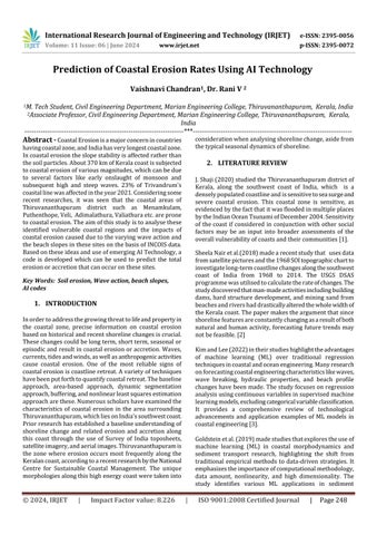
An experimental setup was prepared to analyse wave action's impact on soils. The setup included a wave tank made of glass walls; a wave generator programmed using Arduino UNO, a laptop and a power supply. Experimental setupisshowninFig.1

(a) Experimentalsetup
(b) Experimentalmodelling
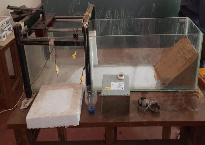
Fig - 3.1: Erosiondegree–30degreesexperimental analysis
The soil slopes of 30 degrees were modelled in the glass tank.Theglasswallswerechosentoresistthewaveimpact aswellastooffereasyvisualanalysisoftheexperiment.The soil samples were mixed in their initial moisture content, compactedandfilledin5layersandtheslopesweremade accordingly.Thewaterlevelwasmaintainedconstantata height of 10cm throughout the experiment. The wave generatoroperatedinthreedifferentvelocitiesi.e.,0.06m/s, 0.07 m/s, 0.08m/s and 0.09m/s respectively. The experimentwasconductedforonehourontheslopeandsoil
sample with varying velocities. The wave height and amplitudewerealsonotedduringtheexperiment.Theinitial heightoftheslopewasnotedandthedifferenceinheights wasnoteddownat0,5,10,15,30,45and60minsrespectively. Thedifferenceinheightofthesoilslopewasusedtofindout the change in the slope angle of the soil slope. The initial massofthesoilsamplewasnotedandtheerodedmasswas also found by calculating the difference between the soil massretainedandthemassinitiallytaken.Erosiondegree, Deisanalysedandfoundoutusingtheformula,De=θ/θ’ Erosion degree is unity when the slope is stable. The reductioninDeindicatesthesoilmassbeingerodedaway.
Artificial intelligence has been used as a tool to solve numericallycomplexproblemswhereanumberofvariables are involved in the field of wave energy and ocean engineering. In recent years, wave height forecasting has been improved by means of diverse artificial intelligence techniques, such as Genetic programming, Neuro wavelet technique, Sequential learning neural networks, Extreme Learning Machine, Bayesian methods, Artificial neural networks.Artificalneuralnetworks(ANNs)ariseasauseful tool as they can deal with non-linear function regression. ANNs can be applied to optimize the coastal protection performance of a wave farm, reducing the computational costofphysically-basednumericalmodels.
Sothecodeiscodedforcalculatingerosiondegreeasfollow: importnumpyasnp
importmath
defcalculate_erosion(initial_slope_degrees, final_slope_degrees,velocity,time_interval):
#Convertslopefromdegreestoradians
initial_slope=math.radians(initial_slope_degrees)
final_slope=math.radians(final_slope_degrees)
#Calculateerosiondegreeusingtheequation:erosion= final_slope/initial_slope
International Research Journal of Engineering and Technology (IRJET) e-ISSN: 2395-0056
Volume: 11 Issue: 06 | June 2024 www.irjet.net p-ISSN: 2395-0072
erosion=final_slope/initial_slope
#Calculatereductionpercentage
reduction_percentage=((initial_slope-final_slope)/ initial_slope)*100
returnerosion,reduction_percentage
#Exampleparameters
initial_slope_degrees=30#Initialbeachslopeindegrees
final_slopes_by_velocity={
0.06:[30,24.62,23.24,21.25,21.21,20.81,20.53],
0.07:[30,22.62,22.08,21.80,21.25,20.70,19.86],
0.08:[30,18.20,16.11,10.08,6.25,5.36,3.20],
0.09:[30,8.53,5.40,2.23,3.18,3.18,3.18]}
time_intervals_minutes_list=[0,5,10,15,30,45,60] # Differenttimeintervalsinminutes
velocities=[0.06,0.07,0.08,0.09] #Differentvelocitiesin m/s
#Calculateerosionfordifferentvelocities,finalslopes, andtimeintervals
erosion_degrees=[] forvelocityinvelocities:
erosion_degree_for_velocity=[]
print(f"Velocity:{velocity}m/s")
print("{:<25}{:<25}{:<20}".format("TimeInterval (minutes)","FinalSlope(degrees)","ErosionDegree")) forfinal_slope_degrees,time_intervalin zip(final_slopes_by_velocity[velocity], time_intervals_minutes_list):
erosion,_=calculate_erosion(initial_slope_degrees, final_slope_degrees,velocity,time_interval)
erosion_degree_for_velocity.append(erosion)
print("{:<25}{:<25}{:<20.3f}".format(time_interval, final_slope_degrees,erosion))
erosion_degrees.append(erosion_degree_for_velocity)
print("\n")
#Calculatereductionpercentagebasedonerosion degreesforthefirstandlastvelocities
reduction_percentages=[] foriinrange(len(time_intervals_minutes_list)):
reduction_percentage=((erosion_degrees[0][i]erosion_degrees[-1][i])/erosion_degrees[0][i])*100
reduction_percentages.append(reduction_percentage)
#Printreductionpercentagetable
print("ReductionPercentage:")
print("{:<25}{:<20}".format("TimeInterval(minutes)", "ReductionPercentage"))
fortime_interval,reduction_percentagein zip(time_intervals_minutes_list,reduction_percentages):
print("{:<25}{:<20.2f}".format(time_interval, reduction_percentage))
the above code will provide the output in tabulated form withtheerosiondegreesandreductionpercentage.
Thefollowingcode,whenincluded,willprovidetheoutput forreductionpercentagecorrespondingtoeachvelocityin graphicaldata
#Plotreductionpercentagesagainsttimeintervalsfor eachvelocity forvelocity,erosion_degree_for_velocityinzip(velocities, erosion_degrees):
plt.plot(time_intervals_minutes_list, erosion_degree_for_velocity,label=f'Velocity:{velocity} m/s')
plt.xlabel('TimeInterval(minutes)')
plt.ylabel('ErosionDegree')
plt.title('ErosionDegreevsTimeInterval')
plt.legend()
plt.grid(True)
plt.show()
© 2024, IRJET | Impact Factor value: 8.226 | ISO 9001:2008
International Research Journal of Engineering and Technology (IRJET) e-ISSN: 2395-0056
Volume: 11 Issue: 06 | June 2024 www.irjet.net p-ISSN: 2395-0072
Forpredictingthetotalerosionoraccretionhappeningat thesitedefinethefollowingaswell;
importmath
defcalculate_erosion_accretion(velocity_data, time_interval,relative_density, original_beach_slope_degrees, erosion_slope_reduction_degrees):
total_erosion=0
total_accretion=0
#Calculatesedimentdensityfromrelativedensity
sediment_density=relative_density*1000 #Densityof wateris1000kg/m^3
foriinrange(len(velocity_data)):
velocity=velocity_data[i]
time=time_interval[i]
erosion_slope_reduction= erosion_slope_reduction_degrees[i]
#Calculatethesloperatiofromtheoriginalbeach slopeindegrees
original_slope_ratio= math.tan(original_beach_slope_radians)
#Assumingerosionandaccretionareproportionalto velocityandadjustedbeachslope
sediment_transport_rate=velocity* reduced_slope_ratio
#Calculateerosionoraccretionforthistimeinterval
erosion_accretion=sediment_transport_rate*time* sediment_density
#Updatetotalerosionoraccretion iferosion_accretion<0:
total_erosion+=abs(erosion_accretion)
else:
total_accretion+=erosion_accretion
returntotal_erosion,total_accretion
Theresultobtainedfortheexperimentistabulatedbelow
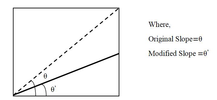
Table 4.1: Erosiondegree–30degrees
From Table 4.1, the extreme case is observed in velocity 0.09m/s after 15 minutes of wave action where the slope notedwasalmost2degrees,Erosiondegreeatthatpointis notedas0.07.After60minutesofexperiment,itisobserved that the erosion degree is reduced by almost 85%. The variationinErosiondegreeof30-degreeslopewithrespect tovariationintimeandvelocitiesareplottedinFig.4.1.
From the graph, it was observed that with the increase in velocity,theerosiondegreedecreaseswhichrepresentsthat theamountofsoilbeingerodedawayincreases.Thisincrease isduetotheincreasedimpactcausedbythewaves.Also,the variationinerosiondegreeisfoundtobemoreintheinitial stagesoftheexperiment.Theerosiondegreeappearstobe morestableinthefinalstageswhichmightbeanindicationof thesoilparticlestryingtoachieveastateofstability.Also,ata higher velocity of 0.09m/s, after 15 minutes some of the
International Research Journal of Engineering and Technology (IRJET) e-ISSN: 2395-0056
Volume: 11 Issue: 06 | June 2024 www.irjet.net p-ISSN: 2395-0072
particlesalreadyerodedawayarefoundtobedepositedin theinitialslopeposition.Thismightbeduetotheswashand backwasheffectofthewaves.
FromtheAICodetheoutputgeneratedisasgivenbelow,
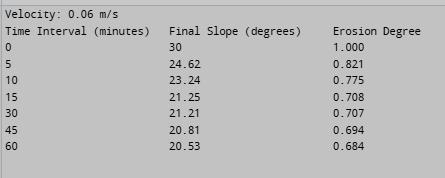
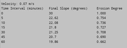
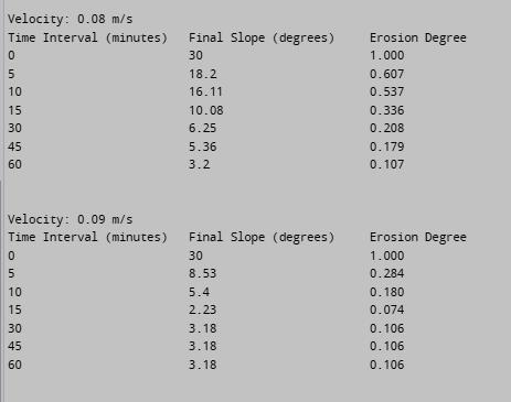
Fig 4.2: Erosiondegree–30degreescodeoutputfor differentvelocitiesandthereductionpercentage
• The erosion degree of soil slopes made in the apparatuswascalculatedfromtheexperiment.
• It is found that increase in velocity decreases erosiondegreewhichindicatesmoreamountofsoil masseroded
• NumericalstudywasconductedusingAIcodesand theerosionratesarecalculated.
• The values of erosion degree obtained from the experiment is comparable to that of the output obtained from the AI code, hence the code is validated
• Similarlythecodecanbeusedtovalidatethedata fordifferentsites
[1] J. Shaji. Coastal sensitivity assessment for Thiruvananthapuram, west coast of India. Natural Hazards 2014,73(3),1369–1392.
[2] L.Sheela Nair,R.Prasad,M.K.Rafeeque, T.N.Prakash. “CoastalMorphologyandLong-termShorelineChanges along the Southwest Coast of India”. Journal of the Geological Society of India 2018,92(5),588–595.
[3] T. Kim, W.-D. Lee. Review on Applications of Machine LearninginCoastal andOceanEngineering. Journal of Ocean Engineering and Technology 2022,36(3),194–210.
[4] E.B.Goldstein,G.Coco,N.G.Plant.Areviewofmachine learningapplicationstocoastalsedimenttransportand morphodynamics. Earth-Science Reviews 2019,194,97–108.