Propagation of Light at the Early Universe Angelo Patrizi and Brett Bochner
Department of Physics and Astronomy The study of the cosmology, mainly the Big Bang Theory, is often a difficult task because no one knows much about what happened at the singularity. Cosmologists try to find a way to eliminate the pre-homogeneous epoch to study what happened before the universe became homogeneous and isotropic. Here we discuss the propagation of light during the early universe and some conclusions drawn from numerical simulation.
Kuang-Li-Liang(KLL) Metric Currently, the universe is homogeneous and isotropic. This implies that anywhere in space is approximately the same temperature, density, and composition in every direction. The Cosmic Microwave Background(CMB) proves this. The CMB is a map of the earliest picture of the entire universe. However, the CMB is radiation from 400,000 years after the start of the universe. To see how light propagated prior to the CMB, two things are required: a model of a pre-homogeneous universe to simulate and mathematical equations that computes the result. The metric used to represent the very early universe is called the Kuang-Li-Liang(KLL) metric. This is a very interesting metric because this metric is nonhomogeneous and filled with pure electromagnetic radiation. Also, this metric is non-vacuum and not flat. This metric represents an expanding but contracting model. The metric is defined as: 2 𝑇±𝑋 𝐽 2 + ⅆ𝑋 2 + 𝑇 ⅆ𝑌 2 + 𝑑𝑍 2 ⅆ𝑠 2 = − ⅆ𝑇 1 𝑇2 This J function satisfies the energy condition J’/J > 0. The J function is shown below: 𝐽 𝑇 ± 𝑋 ∝ ⅇ𝐴 𝑇±𝑋 +𝐵 sin 𝑘𝑠 𝑇±𝑋 Where A ≥ B 𝑘𝑠 .
Electromagnetism in Curved Spacetime Maxwell’s equations are generalized below: 𝜕𝛾 𝐹𝑎𝛽 + 𝜕𝛽 𝐹𝛾𝑎 + 𝜕𝑎 𝐹𝛽𝛾 = 0 𝜕𝑎 𝐹 𝑎𝛽 = 0 Where 𝑎, 𝛽, 𝛾 are t, x, y, or z. Including the KLL metric, the set of equations become: 𝜕𝛾 𝐹𝑎𝛽 + 𝜕𝛽 𝐹𝛾𝑎 + 𝜕𝑎 𝐹𝛽𝛾 = 0
Where Det is the determinant and 𝑔𝜇𝜈 is the KLL metric tensor. The metric tensor is where all the gravitational information about the local curvature is contained. 𝑔𝜇𝜈 is a diagonal matrix with its diagonal values being the coefficients of the spacetime equation on the left. F is the Electromagnetic Tensor which contains information about electromagnetic fields in curved spacetime with gravity(𝑔𝜇𝜈 ). Using the KLL metric, Einstein-Maxwell equations, and a lot of patience, the results are 4th order, uncoupled wave equations in which can be numerically simulated to see how the light propagated in the very early universe. 0
−𝑔𝑡𝑡 𝐸𝑦 −𝑔𝑡𝑡 𝐸𝑧
− 𝑔𝜇𝜈 =
𝑇 0 0 0
0 𝐽2
𝑇 0 0
0
0
0
0
𝑇 0
0 𝑇
𝑎𝛽 𝐹
=
𝜇𝑎 𝛽𝜈 𝑔 𝐹𝑎𝛽 𝑔
𝑔𝜇𝜈 𝑔
𝑎𝛽
=𝐼
− −𝑔𝑡𝑡 𝐸𝑥
−𝑔𝑡𝑡 𝐸𝑥
𝐹𝑎𝛽 =
2 𝐽
−𝐷ⅇ𝑡 𝑔𝜇𝜈 𝐹 𝑎𝛽 = 0
𝜕𝑎
− −𝑔𝑡𝑡 𝐸𝑦 𝑔𝑥𝑥 𝑔𝑦𝑦
0 −
𝑔𝑥𝑥 𝑔𝑦𝑦 𝑔𝑧𝑧
𝑔𝑧𝑧
𝐵𝑧
𝑔𝑥𝑥 𝑔𝑧𝑧 𝐵𝑦 𝑔𝑦𝑦
𝐵𝑧
−
𝑔𝑦𝑦 𝑔𝑧𝑧 𝑔𝑥𝑥
−
𝑔𝑥𝑥 𝑔𝑧𝑧 𝐵𝑦 𝑔𝑦𝑦
𝑔𝑥𝑥
𝐵𝑥
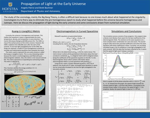
The simulation process consists of two programs. One program does a Monte Carlo Markov Chain search for the best coefficients of the electromagnetic fields. The solutions to the wave equations are a more complex linear combination of a sine and cosine. The second program takes those best searched coefficients and solves the wave equations with those coefficients in them. Currently, runs are being simulated to gain a lot of confidence in how light propagated in the early universe. With the data that has been collected so far, it seems that the speed of light wasn’t always a constant.
− −𝑔𝑡𝑡 𝐸𝑧
𝑔𝑦𝑦 𝑔𝑧𝑧
0
Simulations and Conclusions
0
𝐵𝑥 0.5 , 𝜋
Here is a graph of all the phase velocities with A = 0.6, B = and 𝑘𝑠 = 𝜋. As viewed from the graph, the speed of light exceeds the constant speed of light, c and then dips below c converging to the constant known today. In this picture, the speed of light c = 1 for simplicity. Ideally, the speed of light is close to 3 × 10⁸ m/s.