Greater Yellowstone Climate Assessment

GREATER YELLOWSTONE

CLIMATE ASSESSMENT

Past, Present, and Future Climate Change in Greater Yellowstone Watersheds

This page left to right

first row: Cody WY (photo credit: Wikimedia under Creative Commons); rail-to-trail conversion between Ashland and Driggs ID

second row: pronghorn statues in Pinedale WY; looking west across a portion of Bozeman MT (photos courtesy of Scott Bischke, except as noted)

On the cover

map: created by Emily Reed (using ArcGIS® software, copyright ESRI and used herein under license)

photo: upper Yellowstone River with Electric Peak in the distance and Gardner MT just visible to the right (courtesy of Scott Bischke)

GREATER YELLOWSTONE

CLIMATE ASSESSMENT

Past, Present, and Future Climate Change

in Greater Yellowstone Watersheds

Steven Hostetler 1, Cathy Whitlock 2, Bryan Shuman 3 , David Liefert 4, Charles Wolf Drimal 5, and Scott Bischke 6

1 Co-lead; Research Hydrologist; US Geological Survey Northern Rocky Mountain Science Center, Bozeman MT

2 Co-lead; Regents Professor Emerita of Earth Sciences, Montana Institute on Ecosystems, Montana State University, Bozeman MT

3 Wyoming Excellence Chair in Geology & Geophysics, University of Wyoming, Laramie WY; Director, University of Wyoming-National Park Service Research Center at the AMK Ranch, Grand Teton National Park

4 Water Resources Specialist, Midpeninsula Regional Open Space District, Los Altos CA; PhD graduate, Department of Geology and Geophysics, University of Wyoming, Laramie WY

5 Waters Conservation Coordinator, Greater Yellowstone Coalition, Bozeman MT

6 Science Writer, MountainWorks Inc., Bozeman MT

Land Acknowledgment

The lands and waters of the Greater Yellowstone Ecosystem have been home to Indigenous people for over 10,000 years. In the most recent millennium, over a dozen Tribes have considered this region a part of their traditional (ancestral) homelands. This includes, but is not limited to, several Tribes and bands of Shoshone, Apsáalooke/Crow, Arapaho, Cheyenne and Ute Nations, as well as the Bannock, Gros Ventre, Kootenai, Lakota, Lemhi, Little Shell, Nakoda, Nez Perce, Niitsitapi/Blackfeet, Pend d’Oreille, and Salish. We pay respect to them and to other Indigenous peoples with strong cultural, spiritual, and contemporary ties to this land. We are indebted to their stewardship. We recognize and support Indigenous individuals and communities who live here now, and those with cultural and spiritual connections to these Homelands.

Support for this project came from Montana State University, University of Wyoming, US Geological Survey, Greater Yellowstone Coordinating Committee, and Greater Yellowstone Coalition. Scott Bischke of MountainWorks Inc. (www.emountainworks.com) served as the report science editor, print-copy designer, and website developer.

Greater Yellowstone Climate Assessment: Past, Present, and Future Climate Change in Greater Yellowstone Watersheds is available in digital format at www.gyclimate.org. While included in this report, a stand-alone Executive Summary is also available.

Suggested citation

Hostetler S, Whitlock C, Shuman B, Liefert D, Drimal C, Bischke S. 2021. Greater Yellowstone climate assessment: past, present, and future climate change in greater Yellowstone watersheds. Bozeman MT: Montana State University, Institute on Ecosystems. 260 p. https://doi.org/10.15788/GYCA2021.

Madison River in spring flood, here at 7-mile bridge in Yellowstone National Park, near West Yellowstone MT

Photo courtesy of Scott Bischke

CONTENTS

I EXECUTIVE SUMMARY

II What is the Greater Yellowstone Climate Assessment?

III Major Findings

XVI Implications for the Region

XIX Concerns from Stakeholders

XX Conclusions

XXII Literature Cited

XXIV ACKNOWLEDGMENTS

XXVII LIST OF ACRONYMS

XXVIII FOREWORD

Cam Sholly

1 1. INTRODUCTION TO THE GREATER YELLOWSTONE CLIMATE ASSESSMENT

Cathy Whitlock, Steven Hostetler, and Bryan Shuman

5 The Geography of the Greater Yellowstone Area

8 The HUC6 Watersheds in the GYA

10 Structure of the Assessment

12 Literature Cited

15 2. CLIMATE, CLIMATE VARIABILITY, AND CLIMATE CHANGE IN THE GREATER YELLOWSTONE AREA

Cathy Whitlock, Steven Hostetler, Gregory Pederson, and David Liefert

15 Key Messages

16 What is Climate?

17 Climate and Water Variables Discussed in the Assessment

18 Present Climate

20 Past Climate Change

31 Causes of Climate Change

33 Summary

35 Literature Cited

40 3. HISTORICAL CLIMATE AND WATER TRENDS IN THE GREATER YELLOWSTONE AREA

David Liefert, Bryan Shuman, Steven Hostetler, Rob Van Kirk, and Jennifer L. Pierce

40 Key Messages

41 Introduction

42 Data Sources

44 Historical Climate Changes in the GYA

62 Historical Hydrological Changes in the GYA

71 Summary

73 Literature Cited

79 4. BACKGROUND TO CLIMATE PROJECTIONS

Steven Hostetler

79 Key Messages

79 Introduction

80 Climate Scenarios

82 Climate Models

87 Downscaling Climate Projections

90 Climate Projections Used in the Greater Yellowstone Climate Assessment

91 Summary

92 Chapter 4 Appendix—A Deeper Look

99 Literature Cited

102 5. FUTURE TEMPERATURE PROJECTIONS FOR THE GREATER YELLOWSTONE AREA

Steven Hostetler and Jay Alder

102 Key Messages

102 Details of Temperature Projections

103 Seasonal Temperature Changes Over the GYA

106 Annual Temperature Trends in the Watersheds

108 The Seasonal Cycle of Temperature

110 Temperature Extremes in HUC6 Towns

120 Summary of Projected Temperature Changes

121 Chapter 5 Appendix—A Deeper Look

125 Literature Cited

127 6. FUTURE PRECIPITATION PROJECTIONS FOR THE GREATER YELLOWSTONE AREA

Steven Hostetler and Jay Alder

127 Key Messages

127 Introduction

128 Annual and Seasonal Precipitation Over the GYA

130 Precipitation Over the HUC6 Watersheds

132 The Seasonal Cycle of Precipitation

135 Summary of Projected Precipitation Changes

136 Chapter 6 Appendix—A Deeper Look

138 Literature Cited

139 7. FUTURE WATER PROJECTIONS FOR THE GREATER YELLOWSTONE AREA

Steven Hostetler and Jay Alder

139 Key Messages

141 Introduction 141 Snow

146 Runoff

151 Evapotranspiration and Soil Water

158 Summary

159 Chapter 7 Appendix—A Deeper Look

165 Literature Cited

168 8. VOICES FROM THE GREATER YELLOWSTONE AREA

Charles Wolf Drimal, Ryan Cruz, Allison Michalski, and Emily Reed

168 Key Messages

169 Introduction

171 Stakeholder Concerns

174 Impacts to Stakeholders

177 Current Information

180 Information Needed

184 Leaders and Current Work

186 Project Needs

190 Policy

193 Summary

193 Literature Cited

195 9. CONCLUDING REMARKS

Cathy Whitlock, Steven Hostetler, Bryan Shuman, David Liefert, Charles Wolf Drimal, and Scott Bischke

201 Science and Monitoring Needs

202 Climate Adaptation and Related Needs

203 Literature Cited

204 GLOSSARY

215 BIOGRAPHICAL SKETCHES

215 Contributors

218 Reviewers

Sprinkler irrigation on a potato field east of Ashton, Idaho

Photo courtesy of Brian Apple (Henry’s Fork Foundation)

EXECUTIVE SUMMARY

The Greater Yellowstone Area (GYA) is one of the last remaining large and nearly intact temperate ecosystems on Earth. GYA was originally defined in the 1970s as the Greater Yellowstone Ecosystem, which encompassed the minimum range of the grizzly bear. The boundary now includes about 22 million acres (8.9 million ha) in northwestern Wyoming, south central Montana, and eastern Idaho (Figure ES-1). Two national parks, five national forests, three wildlife refuges, 20 counties, and state and private lands lie within the GYA boundary (Figure ES-1). The Tribal Nations of the Eastern Shoshone, Northern Arapaho, Apsáalooke/Crow, Northern Cheyenne, Shoshone, and Bannock have reservations in and near the Greater Yellowstone Area, and 27 Tribes are formally recognized to have historical connections to the lands and resources of the region. Natural resources sensitive to climate change connect many of the major economic activities of the GYA, including tourism and recreation, agriculture, and energy development.

Outlet of Brewmark Lake, Bridger Wilderness, Wind River Range, Wyoming

Photo courtesy of Bryan Shuman

Figure ES-1. Map of the Greater Yellowstone Area (GYA) showing the six Hydrologic Unit Code 6 (HUC6) watersheds studied under the Assessment, and including mountain ranges, lakes and major river systems, jurisdictions, and selected towns. The portions of the watersheds within the GYA boundary are studied in this report. (Map created using ArcGIS® software, copyright ESRI and used herein under license.)

Humans are contributing substantially to global warming and climate change through greenhouse gas emissions, especially from the burning of fossil fuels (IPCC 2013; USGCRP 2017; Blunden and Arndt 2019). The leading science organizations around the world have issued public statements expressing this finding, including international and United States science academies, the United Nations Intergovernmental Panel on Climate Change, and a host of reputable scientific bodies (IPCC 2013; USGCRP 2017; Blunden and Arndt 2019).

The widespread consensus that the effects of climate change are increasingly apparent in all parts of the planet motivated us to analyze the potential impacts on the climate and water resources of the Greater Yellowstone Area.

WhAT IS ThE Greater Yellowstone Climate assessment?

This first volume of the Greater Yellowstone Climate Assessment (“the Assessment”) presents an in-depth summary of past, historical, and projected future changes to temperature, precipitation, and water in the GYA. It is intended as a basis for further research and discussion of the important impacts and adaptation and mitigation opportunities related to climate change in the region. This Assessment, like others done at the international, national, and state levels, draws on the best science available at the time of writing (see box). To provide geographic detail to the analysis we focus on the GYA and six major river basins within the GYA.

MAjOR FINdINGS

The major findings from the Assessment are summarized in Table ES-1. We provide additional details below. Estimates of confidence are provided for the key messages. They represent confidence that the specific data sets and model results examined here agree upon the direction of change and its significance (see Table 1-2 in the Assessment).

Table ES-1: Major findings of the Greater Yellowstone Climate Assessment for the Greater Yellowstone Area (GYA) and Hydrologic Unit Code 6 (HUC6) watersheds based on observations for the 1950-2018 historical period and projected changes to the year 2100. (RCP stands for Representative Concentration Pathways.)

Change between 1950-2018

Trends to 2100 compared to 1986-2005 (based on MACAv2_METDATA1

1 The MACAv2-METDATA data set includes 20 global climate models that were statistically downscaled to a 4 km by 4 km (2.5 mile by 2.5 mile) grid using the Multivariate Adaptive Constructed Analogs method.

2 Based on April 1st values.

3 At towns in the major watersheds: Bozeman MT, Red Lodge MT, Cody WY, Pinedale WY, Jackson WY, Driggs ID. Base temperature is 45°F (7.2 °C), the germination temperature of wheat.

Historical data reveal how climate trends and extremes can vary geographically within the GYA, but future projections are constrained by the current geographic resolution of the models. Agreement in the future projections across watersheds (Table ES-1) likely underestimates future differences.

How was the Greater Yellowstone Climate Assessment created?

The objective

The Greater Yellowstone Climate Assessment is intended to be a multi-phase effort to analyze and communicate information about climate change in the Greater Yellowstone region. The overarching goals of the Assessment are:

о to present understandable, science-based, and geographically specific information about the potential impacts of climate change on the people and resources of the region; and

о to provide a foundation of knowledge that helps the region prepare for and respond to climate changes occurring within the 21st century.

Water is fundamental for healthy ecosystems, and changes in climate and water affect ecosystem services (e.g., clean air and water, fish, wildlife, forests) in the GYA. The focus of this first volume of the Assessment is to summarize the causes and consequences of past and ongoing climate and hydrologic change on the watersheds of GYA, and to provide projections of future change.

This Assessment—like others done at the international, national, and state level—draws on the best science available at the time of writing to evaluate the state of climate change and its observed and potential impacts. We draw on the science expertise of partner universities, federal and state agencies, and non-governmental organizations, including Montana State University (Montana Institute on Ecosystems), University of Wyoming, Boise State University, US Geological Survey, Yellowstone and Grand Teton national parks, and Henry’s Fork Foundation. An effort to listen to and engage the region’s constituency was led by a team from the Greater Yellowstone Coalition, the Greater Yellowstone Coordinating Committee, National Park Service, the universities and extension services, and the Tribes in Wyoming, Idaho, and Montana.

Prior to release, the Assessment received scientific reviews from experts in the fields of climate, hydrology, and resource management. It also received input from citizens and organizations in the GYA during a period of public comment.

Our analysis

We use the US Geological Survey Hydrologic Unit Code (HUC) watersheds to describe the region because the impact of climate change in the GYA is better characterized by natural geographic boundaries than by artificially defined borders such as state or national park boundaries. In the Assessment, we focus on the six major river basins that meet the definition of HUC level 6 (HUC6) classification: Missouri Headwaters, Upper Yellowstone, Big Horn, Upper Green, Snake Headwaters, and Upper Snake (Figures ES-1 ES-2).

In Chapter 1 we provide an introduction to the GYA and information on the structure of the report, including details on how we assign confidence to our findings. In Chapter 2 we present basic concepts of climate and climate change, summarize past climate and hydrologic changes in the GYA over the last 20,000 yr based on the geological record, and explain the natural and anthropogenic drivers of climate change. In Chapter 3, we examine observed 20th- and early 21stcentury changes and trends in climate and water resources in the GYA based on weather station and streamgage measurements.

In Chapter 4, we provide an overview of the scientific methods used to develop projections of future changes in climate and water. In Chapters 5, 6, and 7, we present 21st-century projections of air temperature, precipitation, and water, respectively, with a focus on climate variables that are relevant to agriculture, energy use, ecosystems, and winter recreation.

In Chapter 8, we offer some of the results of interviews with residents in the Greater Yellowstone Area, including their concerns for the future. In Chapter 9, we identify knowledge gaps and outline the next steps in the assessment process.

Dry periods in the past resulted in a near-century hiatus in eruptions of Old Faithful in the Upper Geyser Basin of Yellowstone National Park. (Photo credit: FDR Library; Creative Commons 2.0)

Figure ES-2. Location of National Weather Service (NWS) weather stations (red +) and US Geological Survey streamgaging stations (blue triangle) that provided the meteorological and streamflow records used in our analysis. We examine weather station data back to 1950 and streamflow data back to 1925.

Temperature

Past perspective

о GYA average temperature of the last two decades (2001-2020) is probably as high or higher than any period in the last 20,000 yr, and likely higher than previous glacial and interglacial periods in the last 800,000 yr. Research suggests that the current level of carbon dioxide in the atmosphere is the highest in the last 3.3 million years. [medium confidence]

о Climate models can only capture the observed global temperature trend from 1880 to present by incorporating natural and anthropogenic drivers, including human-emitted atmospheric greenhouse gases. [high confidence]

Since 1950

о Meteorological records since 1950, averaged across the GYA, show that mean annual temperature in the GYA has increased by 2.3°F (1.3°C) at a rate of 0.35°F (0.20°C) per decade. [high confidence]

Noteworthy:

• The trends are large relative to typical warm- or cold-year departures from the average, of 1.3°F (0.7°C) indicated by the standard deviation since 1950.

• Warming has been more pronounced in spring than other seasons, particularly in March (Figure ES-3).

• Mean annual temperatures in the Missouri Headwaters and Upper Snake watersheds are now similar to those of the Big Horn watershed, which historically was the warmest subregion of the GYA (Figure ES-3 and ES-4).

• In the coolest watershed of the GYA, the Upper Green, annual average temperatures have risen from near freezing in the 1950s to the upper 30s°F (15°C) in the 2010s, causing a reduction in snowfall even though there has been little change in annual precipitation totals.

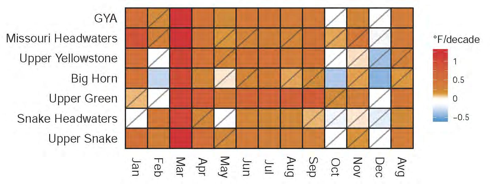
Figure ES-3. Temperature trends from 1950-2018 by watershed and month in the Greater Yellowstone Area (GYA). Boxes without slashes are statistically significant at the 95% confidence level. The last column (Avg) is the mean annual rate of change in each watershed.

Figure ES-4. Annual temperature, total precipitation, and snowfall trends for the Greater Yellowstone Area (GYA) and Hydrologic Unit Code 6 (HUC6) watersheds since 1950. Each dot in the plots represents the mean annual value. The black lines are LOESS regressions fit to the point data and the gray shading indicates the 95% confidence level around the trend LOESS lines. The LOESS fits are used to highlight trends in the data.

Future

In this report we consider two future greenhouse gas emission scenarios, known as Representative Concentration Pathways (RCPs) (see box, Figure ES-5). RCP4.5 describes a moderate greenhouse gas emission scenario assuming significant mitigation of emissions beginning in the next few years. RCP8.5 has little to no mitigation of greenhouse emissions and represents an extreme case. Projections reveal:

о Under RCP4.5 all four seasons warm relative to the 1986-2005 base period. Mean annual temperature in the GYA is projected to increase 5°F (3°C) by the period 20612080 and stabilize thereafter in response to expected mitigation (Figure ES-5). Under RCP8.5 all four seasons warm relative to the 1986-2005 base period and the GYA mean annual temperature is projected to increase by more than 10°F (5.6°C) by the end of the 21st century. [high confidence]

о By the end of the century, the number of hot days per year (high temperature above 90°F [32°C]) is projected to increase and exceed a week in Pinedale WY and a month in Cody WY under RCP4.5. Under RCP8.5, the number of hot days per year increases to nearly two months in Jackson WY and Pinedale WY and exceeds two months in Bozeman MT and Cody WY. [high confidence]

о By the end of the century, the number of cold days (low temperature below 32°F [0°C]) experienced by towns in the major watersheds is projected to decrease by about a month and a half under RCP4.5 and up to two and a half months under RCP8.5. [high confidence]

Precipitation

Past perspective

After the last extended dry period from 1905-1945, which included the 1930s Dust Bowl drought, mean annual precipitation in the GYA has been near to or above the long-term average with substantial year-to-year and decadal variability. For example, low precipitation in 1988 was

Figure ES-5. Historical and projected changes in the Greater Yellowstone Area annual temperature from 1900-2100 plotted as departures from the 1900-2005 PRISM mean (PRISM Climate Group undated). Historical changes in temperature (black line) are described in Chapter 2, and future projections from Representative Concentration Pathway 4.5 (RCP4.5, blue line) and RCP8.5 (red line) are described in Chapter 5. The colored lines for the RCP data are the median of 20 global climate model (GCMs) in the MACAv2-METDATA downscaled data set and the respective shaded bands around the lines are the 10th (lower) and 90th (upper) percentiles of the models.

Future scenarios

The future climate scenarios we use in this Assessment were developed for the Intergovernmental Panel on Climate Change (IPCC) Fifth Assessment Report (IPCC 2013) and are called Representative Concentration Pathways (RCPs). RCPs are a reference to the extent that the accumulation of greenhouse gases (GHGs) and aerosols in the atmosphere affect the balance of incoming and outgoing energy in the Earth system. The number of an RCP indicates the amount of radiative forcing (in watts per square meter, or W/m2) at the year 2100. The higher the RCP value, the greater the potential warming.

The RCPs bracket a range of plausible atmospheric GHG concentrations in the future based on various levels of emission reductions (mitigation), without assigning likelihood to any pathway. We base the Assessment on RCP4.5 and RCP8.5. RCP4.5 is an intermediate pathway that results in about 4.5°F (2.5°C) of global warming by the end of the century. RCP8.5 is an upper bound pathway that represents little or no mitigation in the coming decades and results in global warming of about 9°F (5°C) by the end of century. RCP4.5 and RCP8.5 are currently the most widely considered scenarios in climate change research.

this is dummy text RCP8.5

Annual average atmospheric CO2 concentrations. The black line combines reconstructed values from 1880-1958 and Mauna Loa observations from 1959-2019. The colored lines are the four Representative Concentration Pathway (RCP) scenarios used in the Fifth IPCC Assessment Report (2013). Mauna Loa observations retrieved from Scripps Institute (undated). RCP2.6 data from van Vuuren et al. (2007); RCP4.5 data from Smith and Wigley (2006), Clarke et al. (2007), and Wise et al. (2009); RCP6.0 data from Fujino et al. (2006) and Hijioka et al. (2008); RCP8.5 data from Riahi et al. (2007). These data sources are compiled at RCP Database (undated).

followed by several years of high precipitation during the late 1990s and then very dry years in 2005 and 2016. The geologic record indicates that decade-long periods of low precipitation have occurred in the past 1200 yr. These dry periods were times of reduced snowpack, more fires, lower streamflow, establishment of trees above present tree line, and even a near-century hiatus in geyser activity of Old Faithful.

Since 1950

о Average precipitation across the GYA has not changed significantly and remains near 15.9 inches (40.5 cm) with year-to-year variability of 2.2 inches (5.6 cm) based on the standard deviation of the meteorological record average. [high confidence]

о Precipitation has increased in spring and fall, by 17-23% in April and May, and 42% in October. It has declined by 17% in June and 11% in July. [high confidence]

о As climate has warmed, mean annual snowfall in the GYA has declined by 3.5 inches (8.9 cm) per decade. [medium confidence]

Noteworthy: In the wettest watershed of the GYA, the Snake River headwaters, annual precipitation has increased, but annual snowfall has declined.

о Much of the snowfall decline has occurred in spring when warming was greatest. [high confidence]

Noteworthy:

• Measurable snowfall has become rare in June and September as the snow-free season has lengthened.

• Average snowfall at weather stations in the GYA used to be highest between 60007000 ft (1800-2100 m) elevation, but since 1950, snowfall in this elevation range has declined markedly even as total annual precipitation has remained the same or increased. The decline has occurred because mean temperature has risen by 2.5°F (1.4°C) since the 1980s over those elevations, which converted precipitation from snow to rain.

Figure ES-6. The 1986-2099 annual snow regime for the Greater Yellowstone Area (GYA) and Hydrologic Unit Code 6 (HUC6) watersheds under RCP4.5. The five maps across the top display SWE:P, which is the ratio of snow (measured as snow water equivalent [SWE]) to rain during the cold-season (Oct-Apr). The pie charts inset in the maps show the fraction of the GYA within each snow-to-rain category. The time-elevation plots for the HUC6 watersheds in the bottom two rows display the trend in each category from 1986-2099 averaged over 330 ft (100 m) elevation bands. Gray shading indicates elevations not present in the HUCs. (The appendix to Chapter 7 provides more details on the SWE:P ratio, and the related figure for Representative Concentration Pathway 8.5 [RCP8.5].)

Future

о Under RCP4.5, mean annual precipitation in the GYA is projected to increase 7% by mid century (2041-2060) and 8% by the end of century (2081-2099) relative to the 19862005 base period. Under RCP8.5, the projected increases are 9% and 15% for these periods, respectively. [high confidence]

о The projected increase in mean annual precipitation is attributed to increases during the December through April cold season, particularly in March and April when the snow-to-rain transition occurs. [high confidence]

о By the end of the century (2081-2099), the wettest month shifts from May to April in the Big Horn, Upper Green, and Snake Headwaters HUC6 watersheds. These shifts occur by mid century (2061-2080) and are amplified under RCP8.5. [medium confidence]

о Under RCP4.5, the total area of the GYA dominated by winter snowfall decreases from 59% during the base period (1986-2005) to 27% mid century (2041-2060) and to 11% by the end of century (2081-2099). Under RCP8.5, the extent of snow-dominant area decreases to 17% and to 1% for the same time periods, respectively (Figure ES-6) [high confidence]. These changes result in a decrease in the amount of water stored as annual snowpack (Figure ES-7).

Figure ES-7. Changes in the amount of water (SWE) stored in the April 1 snowpack in the Greater Yellowstone Area relative to the 1950-2005 mean as simulated by the water balance model used in the Assessment. Historical changes (black line), Representative Concentration Pathway 4.5 (RCP4.5, blue line), and RCP8.5 (red line) are the median change for the 20 global climate models (GCMs) in the MACAv2-METDATA data set as described in Chapter 7. The respective shaded bands around the lines are the 10th (lower) and 90th (upper) percentiles of the models.

Streamflow, runoff, and soil water deficit

Streamflow records in the GYA since the early 20th century allow comparison of current trends to past events such as the 1930s Dust Bowl drought. Hydrologic simulations enable projections of streamflow, runoff, and soil moisture based on the climate projections.

Since 1925

о Annual streamflow today is similar to that of the mid-20th century, but on average over the GYA the timing of peak flow has shifted earlier in the year by by 8 days (range of 1-15 days in the HUC6 watersheds), extending the length of the water-limited warm season. [high confidence]

Noteworthy:

• The shift in the timing of peak streamflow since 1970 has been approaching the early timing that occurred during the 1930s Dust Bowl drought. The recent shift, however, is caused by rising spring temperatures that melt snow earlier, whereas during the Dust Bowl drought it was caused by a year-round decline in precipitation.

Bison on Yellowstone’s Northern Range

Photo courtesy of Cindy Goeddel

• The volume of streamflow in most of the rivers has changed little relative to the average conditions of the last 95 yr, but increases in some rivers, such as the Yellowstone, Gallatin, and Madison, contribute to a regional average increase in streamflow of less than 10% since 1925.

• In selected free-flowing rivers within the GYA, annual flows since the mid-20th century have decreased by 3-11%, spring flows have increased by 30-80%, and summer and fall minimum flows have declined by 10-40% (Figure ES-8).

Figure ES-8. Monthly mean streamflow in free-flowing rivers in the Greater Yellowstone Area from 1985-2018 (left column), and percent changes from the 1950-1984 average (right column; the averaging period for the South Fork Shoshone is 1960-1989). The asterisks indicate changes that are statistically significant at a 90% level (based on a means t-test). The inset numbers are the percent change in mean annual flow. The rivers are selected based on USGS streamgages identified in the USGS Hydro-Climate Data Network as having little or no human impact on natural flow (Lins 2012).

Future

о Total annual runoff in the GYA is projected to increase by about 1% by mid century (2041-2060) and by 2% at the end of century (2081-2099) under RCP4.5 and increase by 2% and 3% for same time periods, respectively, under RCP8.5. [low to medium confidence]

о The seasonality of runoff is projected to change as snowfall declines and snowpack melts earlier under both RCP4.5 and RCP8.5. [high confidence]

Noteworthy:

• The biggest changes will be at mid- and high elevations where runoff from snowmelt increases in spring (March through May) and decreases in summer (June through August).

• Timing of peak runoff is projected to shift 1-2 months earlier in the year in the later part of the century under RCP8.5.

о On an annual basis, precipitation (P) over the GYA exceeds potential evapotranspiration (PET), but the reverse is true in summer, particularly at lower elevations, leading to a seasonal water deficit that is projected to increase in the future. [high confidence]

Noteworthy: Under RCP4.5, the summer water deficit is projected to increase by 25% mid century and by 36% by the end of century. Under RCP8.5, projected deficit increases are 35% by mid century and 79% by the end of century.

о Under RCP4.5 June-October soil moisture saturation decreases by 23% by mid century and 33% by the end of the century. Under RCP8.5 June-October soil moisture saturation decreases by 30% mid century and 56% by the end of the century. [high confidence]

Noteworthy: The declines will reduce already limited soil moisture in summer, which in recent decades (1986-2005) has reached about 25% of capacity at low elevations of the GYA and about 50% of capacity at higher elevations.

IMpLICATIONS FOR ThE REGION

Agriculture

The growing season in the GYA—based on temperature and as represented by the towns in the watersheds (Table ES-1)—is about 2 weeks longer now than it was in the 1950s and is projected to be longer and warmer in the future. Recent climate assessments for the Northern Great Plains (Conant et al. 2018) and Montana (Whitlock et al. 2017) suggest the likelihood of both positive and negative impacts on regional agriculture in the future, but the high elevation and diverse topography of the GYA may be somewhat buffered from the negative impacts that are

projected, for example, in the Great Plains. The greenhouse effect of elevated CO2 levels offers the opportunity to grow new plant varieties, and the likelihood of earlier green-up means an earlier grazing season. Still, while some crops and livestock may benefit from longer, warmer growing seasons in the GYA, irrigated and non-irrigated production will need to accommodate earlier snowmelt and timing of runoff and reduced late-season soil moisture. Warmer conditions may also decrease forage quality and support an increase in crop pests.

Energy

Future warming in winter will decrease annual heating degree days in the GYA, which will lessen energy demand for commercial and home heating. Relative to the 1986-2005 base period, under RCP4.5 heating degree days decrease by 13% by mid century (2041-2060) and decrease by 14% by the end of century (2080-2099) (Figure ES-9). Under RCP8.5, decreases are 16 and 31% for the two periods, respectively. By mid century, under both RCPs the projected decrease in heating degree days in the towns is roughly five times greater than the increase in cooling degree days, which would mean less annual energy use in the future.

Figure ES-9. Annual number of heating degree days (top two rows) and cooling degree days (bottom two rows) in the Greater Yellowstone Area. The 1986-2005 base periods are shown in the left column and changes for the four future periods are shown to the right. The mapped data are computed from MACAv2-METDATA daily average minimum temperature (heating degree days) and daily average maximum temperature (cooling degree days).

Wildfire

In the future, earlier snowmelt and loss of snowpack, as a result of warming winters, followed by warmer summers, longer growing seasons, and reduced water availability will increase fire potential at all elevations of the GYA (Westerling et al. 2011). This condition, combined with increased tree mortality, potentially could alter future fire regimes and lead to rapid changes in forest ecosystems. Sustained changes in climate and fire disturbance will also affect the recovery of species after fire, changing forest composition, and possibly converting forest to grassland at low elevations. Thus, increased fire activity portends large ecological changes and threatens human health and the communities in the GYA.

Winter recreation

Decreases in snowpack are projected to continue in the future. Even though precipitation is projected to increase, as winters warm, a smaller portion of precipitation will fall as snow and more will be a mixture of rain and snow, particularly in March and April when the snow-rain transition now occurs. Under RCP4.5, mid-century loss of snowpack ranges between 24-31% of 1986-2005 levels and reaches 38-44% by the end of century. Losses are greater under the warmer conditions of RCP8.5. Elevational changes in snow will affect most aspects of winter recreation in the GYA. In Yellowstone National Park, for example, Tercek and Rodman (2015) found that the length of the snow season at the end of century (2061-2090) could decline by 16 and 27% from present under RCP4.5 and RCP8.5, respectively, with similar or greater declines in the number of days suitable for over-snow vehicles. Lackner et al. (2021) project that under RCP8.5 the number of ski days in 2050 will be reduced by from 6 to 29 days at ski areas within the GYA.

CONCERNS FROM STAkEhOLdERS

The GYA is home to a great diversity of species and environments and a rich variety of cultures. Interviews conducted with 44 stakeholders throughout the GYA yielded important insights into the climate realities faced by local communities. Participants spoke about their perspectives on climate change, providing their concerns, observations, and priorities for the future. The following key findings emerged from these conversations:

о Water issues are at the core of climate change impacts in the GYA. Communities and managers will continue to face challenges like drought and shifts in seasonal water cycles in the future.

о Participants’ understanding of and response to climate change is driven more by their background (stakeholder group) than their location (watershed).

о A pressing need exists for a climate information hub that is comprehensive, collaborative, accessible, and useful to experts and the public alike.

о For the most part, meaningful policy to address and adapt to climate change is lacking in the GYA.

о By addressing water issues like availability and quality in future climate adaptation work, we stand to have positive impacts on myriad other conditions including wildlife habitat, fisheries health, and the economy of local communities.

Photos courtesy of, from left to right: #1,4 Greater Yellowstone Coalition; #2 Charles Wolf Drimal; #3 Bryan Shuman

CONCLuSIONS

This first-phase Assessment provides an overview of the potential impacts of climate change in GYA watersheds. It is intended as a starting point for future assessments focused on related topics, including impacts on water, fish and wildlife, local economies and communities, and human health in the GYA.

We conclude the report by identifying some of the important gaps in our scientific understanding of climate change in the GYA. We also highlight needs for climate adaptation efforts. These lists are not exhaustive but are intended to highlight issues we believe deserve attention in future assessments and planning efforts.

Science and monitoring needs

о Provide regular updates of the Greater Yellowstone Climate Assessment that incorporate the latest climate projections consistent with those developed at the national and international level.

о Develop and apply more detailed models of snow processes, groundwater, surface water, and ecosystem and human water demand to refine our understanding of water and water use in the GYA. Modeling potentially complex local changes in water supply, demand, and their interactions will require improved representations of the underlying processes in each watershed.

о Maintain and expand monitoring of snow, streams, lakes, and wetlands within GYA watersheds. Currently, weather stations and streamgages are unevenly distributed in the GYA, few water bodies and wetlands are monitored, particularly at high elevations, and water demand for ecosystems and for human use and consumption is poorly measured.

о Quantify the connections between climate change, the carbon cycle, urbanization, agricultural practices, and biodiversity in the GYA. This information will help identify opportunities to maintain valued ecosystem qualities and services, sustain essential economic and cultural uses, and increase carbon storage on natural and managed lands.

о Continue to expand monitoring efforts of fish and wildlife to improve our understanding of their changing behavior, disease, and distribution in response to climate change.

о Continue to improve our understanding of the linkages between long-term trends in fire climate and short-term fire weather and fuel conditions.

о Support studies of forest health, including the impact of climate change on insect outbreaks, wildfire activity, drought-caused mortality, and carbon storage to guide appropriate management planning.

о Quantify how climate change in the GYA will affect vital ecosystem services, including air quality, water quality and quantity, food, timber, and biodiveristy.

Climate adaptation needs

о Expand efforts to engage regional stakeholders on the topic of climate change through listening sessions and other exchanges that help find common ground for effective watershed and community planning. Establish effective ways to share information from new scientific studies and from monitoring and evaluation efforts so that it is available to all stakeholders in a timely way.

о Work with communities and water management districts to identify the local consequences of climate change, as a step toward developing implementing adaptation plans. On tribal lands, sustaining traditional subsistence, ceremonial, and medicinal resources is also important. Identify crossjurisdictional challenges early in the process, so that planning efforts are effective and efficient.

о Develop a list of at-risk habitats and specific indicators of ecological and human health to be studied and monitored to help resource managers maintain a robust baseline for measuring change and assessing the effectiveness of adaptation measures.

о Evaluate the effects of projected climate change on the economies of the GYA: tourism and recreation, hunting and fishing, agriculture and forestry, and mineral and energy resource extraction as part of a sustained Assessment effort.

Arapaho Color Guard at Northern Arapaho bison release in 2019, Ethete WY

Photo courtesy of Crystal C’Bearing

LITERATuRE CITEd

Blunden J, Arnd DS (editors). 2019. State of the climate in 2018. Bulletin of the American Meteorological Society 100(9):Si–S306. Available online https://doi.org/10.1175/2019BAMSStateoftheClimate.1. Accessed 13 May 2021.

Clarke L, Edmonds J, Jacoby H, Pitcher H, Reilly J, Richels R. 2007. Scenarios of greenhouse gas emissions and atmospheric concentrations: sub-report 2.1A of synthesis and assessment product 2.1 by the US Climate Change Science Program and the Subcommittee on Global Change Research. Washington DC: Department of Energy, Office of Biological & Environmental Research. 154 p.

Conant RT, Kluck D, Anderson M, Badger A, Boustead BM, Derner J, Farris L, Hayes M, Livneh B, McNeeley S, Peck D, Shulski M, Small v. 2018. Northern Great Plains [chapter 22]. In: Impacts, Risks, and Adaptation in the United States: Fourth National Climate Assessment, vol II. In: Reidmiller DR, Avery CW, Easterling DR, Kunkel KE, Lewis KLM, Maycock TK, Stewart BC, editors. Washington DC: US Global Change Research Program. p 941-86. https://doi.org/10.7930/NCA4.2018.CH22.

Fujino J, Nair R, Kainuma M, Masui T, Matsuoka Y. 2006. Multi-gas mitigation analysis on stabilization scenarios using AIM global model. The Energy Journal 3:343-54.

Hijioka Y, Matsuoka Y, Nishimoto H, Masui M, Kainuma M. 2008. Global GHG emissions scenarios under GHG concentration stabilization targets. Journal of Global Environmental Engineering 13:97-108.

[IPCC] International Panel on Climate Change. 2013. In: Stocker TF, Qin D, Plattner G-K, Tignor M, Allen SK, Boschung J, Nauels A, xia Y, Bex v, Midgley PM. editors. Climate change 2013: the physical science basis. Contribution of Working Group I to the Fifth Assessment Report of the Intergovernmental Panel on Climate Change. Cambridge UK and New York NY: Cambridge University Press. 1535 p. Available online https://www.ipcc.ch/report/ar5/wg1/. Accessed 8 Mar 2021.

Lins HF. 2012. USGS HHydro-Climatic Data Network 2009 (HCDN–2009). US Geological Survey fact sheet 2012-3047. 4 p. Available online https://pubs.usgs.gov/fs/2012/3047/. Accessed 20 Dec 2020.

Lackner CP, Greets B, Wang Y. 2021 (Mar 19). Impact of global warming on snow in ski areas: a case study using a regional climate simulation over the interior western United States Journal of Applied Meteorology and Climatology. Available online only. doi:10.1175/JAMC-D-20-0155.1.

PRISM Climate Group. [undated]. PRISM climate data [website]. Available online https://prism.oregonstate. edu/. Accessed 5 Jan 2021.

RCP Database. [undated]. RCP database version 2.05 [website]. Available online https://tntcat.iiasa.ac.at/ RcpDb/. Accessed Oct 2020.

Riahi K, Gruebler A, Nakicenovic N. 2007. Scenarios of long-term socio-economic and environmental development under climate stabilization. Technological Forecasting and Social Change 74(7):887-935.

Scripps Institute. [undated]. Atmospheric CO2 data: primary Mauna Loa CO2 record [webpage]. Accessible online https://scrippsco2.ucsd.edu/data/atmospheric_co2/primary_mlo_co2_record.html. Accessed 29 Mar 2021.

Smith SJ, Wigley TML. 2006. Multi-gas forcing stabilization with the MiniCAM. The Energy Journal 3:373-91.

Tercek MT, Rodman AW. 2015. Forecasts of 21st-century snowpack and implications for snowmobile and snowcoach use in Yellowstone National Park. PLOS One 11. https://doi.org/10.1371/journal. pone.0159218.

[USGCRP] US Global Change Research Program. 2017. Wuebbles DJ, Fahey DW, Hibbard KA, Dokken DJ, Steward BC, Maycock TK, editors. Climate science special report: fourth national climate assessment, vol 1. Washington DC: USGCRP. 470 p. doi:10.7930/J0J964J6.

van vuuren D, den Elzen M, Lucas P, Eickhout B, Strengers B, van Ruijven B, Wonink S, van Houdt R. 2007. Stabilizing greenhouse gas concentrations at low levels: an assessment of reduction strategies and costs. Climatic Change 81:119-59. doi:10.1007/s10584-006-9172-9.

Westerling AL, Turner MG, Smithwick EAH, Romme WH, Ryan MG. 2011. Continued warming could transform Greater Yellowstone fire regimes by mid-21st century. Proceedings of the National Academy of Sciences USA 108:13165-70. https://doi.org/10.1073/pnas.1110199108.

Whitlock C, Cross W, Maxwell B, Silverman N, Wade AA. 2017. 2017 Montana Climate Assessment. Bozeman and Missoula MT: Montana State University and University of Montana, Montana Institute on Ecosystems. 318 p. doi:10.15788/m2ww8w.

Wise MA, Calvin Kv, Thomson AM, Clarke LE, Bond-Lamberty B, Sands RD, Smith SJ, Janetos AC, Edmonds JA. 2009. Implications of limiting CO2 concentrations for land use and energy. Science 324:1183-6.

ACKNOWLEDGMENTS

The authors of this report acknowledge the many individuals and organizations who provided input and inspiration for the Assessment. We greatly appreciate your help. We list them alphabetically below, with a special callout to those individuals who completed a technical review of a late draft version of the Assessment.

Jake Bell, Adaptation International, Austin, Tx

L. Whitley Binder, University of Washington Climate Impacts Group, Seattle WA

Bob Crabtree, Chief Scientist, Yellowstone Ecological Research Center, Bozeman, MT

David Diamond, Executive Coordinator, Greater Yellowstone Coordinating Committee, Bozeman, MT

K. Dello, Oregon Climate Change Research Institute, Corvallis OR

John Doyle, Crow Tribal Elder, Director and Principal Investigator, Crow Water Quality Project, Crow Environmental Health Steering Committee, Little Big Horn College, Crow Agency, MT

Watershed restoration work along the Ruby River, Montana

Photo courtesy of Greater Yellowstone Coalition

Margaret Eggers, Research Assistant Professor of Environmental Health, Montana State University, Bozeman MT

Scott Hauser, Upper Snake River Tribes Foundation, Boise, ID

Julia Hobson Haggerty, Director, Montana Institute on Ecosystems, Montana State University, Bozeman, MT

Jackie Klancher, Professor of Environmental Health & Director of Alpine Science Institute, Central Wyoming College, Riverton, WY

Meade Krosby, University of Washington Climate Impacts Group, Seattle, WA

JoRee LaFrance, Doctoral Student, University of Arizona, Tucson, AZ

Myra Lefthand, MSW, Member, Crow Environmental Health Steering Committee, Little Big Horn College, Crow Agency, MT

Kristin Legg, Ecologist/Manager, Greater Yellowstone Network, National Park Service, Bozeman, MT

W. Andrew Marcus, Director, Atlas of Yellowstone project, University of Oregon, Eugene, OR

Wes Martel, Eastern Shoshone/Northern Arapaho, Senior Wind River Conservation Associate, Greater Yellowstone Coalition, Fort Washakie, WY

Christine Martin, JS. Program Coordinator and US Department of Agriculture Principal Investigator, Crow Water Quality Project, Crow Environmental Health Steering Committee, Little Big Horn College, Crow Agency, MT

Cary Mock, Professor, University of South Carolina, Columbia, SC

Harriet Morgan, University of Washington Climate Impacts Group, Seattle, WA

Alexander (Sasha) Petersen, Adaptation International, Austin, Tx

Andrew Ray, Aquatic Ecologist, National Park Service, Bozeman, MT

Hillary Robison, Yellowstone Center for Resources, Yellowstone National Park, Mammoth, WY

Ann Rodman, Yellowstone Center for Resources, Yellowstone National Park, Mammoth, WY

David Rupp, Oregon Climate Change Research Institute, Corvallis, OR

Naomi Schadt, former MA student, Montana State University, Bozeman, MT

D. Sharp, Oregon Climate Change Research Institute, Corvallis, OR

Alethea Steingisser, Atlas of Yellowstone Project, University of Oregon, Eugene OR

Julia Stuble, Wyoming Public Lands and Energy Associate, The Wilderness Society, Jackson WY

David Thoma, Landscape Ecologist, National Park Service, Bozeman, MT

Emery Three Irons, Crow Environmental Health Steering Committee, Little Big Horn College, Crow Agency, MT

Paige Tolleson, Project Manager, Montana Institute on Ecosystems, Montana State University, Bozeman, MT

Michelle Uberuaga, Executive Director, Park County Environmental Council, Livingston, MT

Sara Young, Crow Environmental Health Steering Committee, Little Big Horn College, Crow Agency, MT

The authors also thank the many photographers, named throughout the report, who have kindly allowed us to use their images.

REvIEWERS

Stephen Gray, PhD, USGS Director of the Alaska Climate Adaptation Science Center, Fairbanks, AK

Greg J. McCabe, PhD, Research Scientist and Hydroclimatologist, US Geological Survey, Denver, CO

Tom Olliff, Intermountain Region Chief, Landscape Conservation and Climate Change, National Park Service, Bozeman, MT

Adam Terando, PhD, Research Ecologist, USGS Southeast Climate Adaptation Science Center, Raleigh, NC

LIST OF ACRONYMS

AMO — Atlantic Multi-decadal Oscillation

AR5 — refers to the Fifth Assessment Report of the IPCC

BSU — Boise State University

CMIP5 — fifth Coupled Model Intercomparison Project

ENSO — El Niño-Southern Oscillation

GCM — global climate model

GHG — greenhouse gas

GYA — Greater Yellowstone Area

GYC — Greater Yellowstone Coalition

HUC — Hydrologic Unit Code

IPCC — Intergovernmental Panel on Climate Change

MCA — Montana Climate Assessment

MSU — Montana State University

NOAA — National Aeronautic and Atmospheric Administration

NPS — National Park Service

NWS — National Weather Service

PDO — Pacific Decadal Oscillation

PDSI — Palmer Drought Severity Index

RCP — Representative Concentration Pathway

SNOTEL — snow telemetry

SNR — signal-to-noise ratio

SWE — snow water equivalent

USGS — United States Geological Survey

UW — University of Wyoming

FOREWORD

Cam Sholly

Superintendent, Yellowstone National Park (2018-present), Chair, Greater Yellowstone Coordinating Committee (GYCC) (2020- 2022)

June 2021

Climate change is one of the biggest threats to transboundary conservation efforts within the Greater Yellowstone Area (GYA). The Greater Yellowstone Climate Assessment is an excellent synthesis of the best available science and serves as a basis for discussion and common understanding among agencies, organizations, and the public in finding solutions to climate change at a regional scale.

The report was produced by researchers from the universities in Montana, Wyoming, and Idaho, partnering with scientists from the US Geological Survey and National Park Service. It will be a much-needed source of climate change information for diverse groups in the region, including private landowners, communities, policy makers, natural resource specialists, and non-profit organizations. Its coverage of past, present, and future climate change and water resources in the GYA provides baseline information for future assessments of the climate impacts on fish, wildlife and forests in the region, as well as our social-economic well-being and human health.

Impacts to water and other natural resources in the GYA associated with climate change are often unidirectional and push the bounds of historic trends. Reframing our priorities and future resource goals is one of our biggest challenges. We know from the Assessment, for example, that temperatures in the GYA have increased by 0.35°F/decade since 1950 and are projected to increase at a higher rate in the future. Warmer temperatures have already led to decreased snowpack at elevations ranging from 5000 to 7000 ft, drier conditions conducive to fire, widespread die-offs of mature whitebark pine trees, invasive species outbreaks, and changes in the timing and rate of snowmelt are affecting fish spawning and the health of aquatic systems. Grassland habitats are altering bison migratory patterns, and rising temperatures are affecting food availability for songbirds. Protecting and restoring corridors (passageways that connect habitat patches) and connectivity across landscapes will require strong collaboration with partners and programs—public and private—throughout the GYA and beyond. These partners must share knowledge, ensure the survival of native species, and develop meaningful cross-jurisdictional conservation priorities and tools to address climate change threats across the ecosystem.

Climate change impacts are not just environmental. Every year, millions of visitors from across the world come to Yellowstone to see the park’s awe-inspiring landscapes and wildlife and spend hundreds of millions in local economies. The communities within the GYA are experiencing rapid growth as people move to the region to enjoy the amenities. Climate impacts throughout the GYA, if not addressed, will directly affect the strength of local and regional economies as resource values and use change across the region.

To mitigate the impacts, Yellowstone National Park and its partners are developing climate response strategies that better incorporate climate data and projections into planning, operations, and program management efforts. We continue to develop new tools to provide realistic assessments of climate vulnerabilities and coordinate actions needed to better understand and respond to these changes.

I recommend the Greater Yellowstone Climate Assessment to you as the current definitive source of how climate change is affecting the GYA. The Assessment makes clear that the scale of climate change impacts far exceeds the ability of any one park, agency, organization, or community to effectively respond as a single entity. Integrated, cooperative adaptation strategies across large geographic areas will lead to more informed, comprehensive, and successful results.

Grand Canyon of the Yellowstone River in Yellowstone National Park

Photo courtesy of Cathy Whitlock

Figure 1-1. Map of the Greater Yellowstone Area (GYA) showing the six Hydrologic Unit Code 6 (HUC6) watersheds studied under the Assessment, and including mountain ranges, lakes and major river systems, jurisdictions, and selected towns. The portions of the watersheds within the GYA boundary are studied in this report. (Map created using ArcGIS® software, copyright ESRI and used herein under license.)

The Greater Yellowstone Area (GYA) is one of the last remaining large and nearly intact temperate ecosystems on Earth…. GYA, and especially the national parks, have long been a place for important scientific discoveries, an inspiration for creativity, and an important national and international stage for fundamental discussions about the interactions of humans and nature.

1. INTRODUCTION TO THE GREATER YELLOWSTONE CLIMATE ASSESSMENT

Cathy Whitlock, Steven Hostetler, and Bryan Shuman

The Greater Yellowstone Area (GYA) is one of the last remaining large and nearly intact temperate ecosystems on Earth (Reese 1984; NPSa undated). GYA was originally defined in the 1970s as the Greater Yellowstone Ecosystem, which encompassed the minimum range of the grizzly bear (Schullery 1992). The boundary was enlarged through time and now includes about 22 million acres (8.9 million ha) in northwestern Wyoming, south central Montana, and eastern Idaho. Two national parks, five national forests, three wildlife refuges, 20 counties, and state and private lands lie within the GYA boundary (Figure 1-1). GYA also includes the Wind River Indian Reservation, but the region is the historical home to several Tribal Nations (see box).

Federal lands managed by the US Forest Service, the National Park Service, the Bureau of Land Management, and the US Fish and Wildlife Service amount to about 64% (15.5 million acres [6.27 million ha] or 24,200 square miles [62,700 km2]) of the land within the GYA. The federal lands and their associated wildlife, geologic wonders, and recreational opportunities are considered the GYA’s most valuable economic asset. GYA, and especially the national parks, have long been a place for important scientific discoveries, an inspiration for creativity, and an important national and international stage for fundamental discussions about the interactions of humans and nature (e.g., Keiter and Boyce 1991; Pritchard 1999; Schullery 2004; Quammen 2016).

Yellowstone National Park, established in 1872 as the world’s first national park, is the heart of the GYA. Grand Teton National Park, created in 1929 and expanded to its present size in 1950, is located south of Yellowstone National Park1 and is dominated by the rugged Teton Range rising from the valley of Jackson Hole. The Gallatin-Custer, Shoshone, Bridger-Teton, Caribou-Targhee, and Beaverhead-Deerlodge national forests encircle the two national parks and include the highest mountain ranges in the region. The National Elk Refuge, Red Rock Lakes National Wildlife Refuge, and Grays Lake National Wildlife Refuge also lie within GYA.

1 Yellowstone and Grand Teton national parks are connected by another unit of the national park system, the 23,000 acre (9300 ha) John D. Rockefeller, Jr. Memorial Parkway.

The People of the GYA

W. Andrew Marcus, University of Oregon

People have lived in the GYA as far back as 12,500 yr ago (Rasmussen et al. 2014) and actively used the resources of the region for millennia (MacDonald 2012). Today, 27 Tribes are formally recognized to have connections to the lands and resources of the region (NPSb undated), including, but not limited to, several Tribes of Shoshone, Bannock, Lemhi, Niitsitapi/Blackfeet, Nez Perce, Salish, Apsáalooke/Crow, Arapaho, Pend d’Oreille, Kootenai, Gros ventre, Assiniboine, Sioux, Little Shell, Northern Cheyenne, and Chippewa Cree. The Tribal Nations of the Eastern Shoshone, Northern Arapaho, Apsáalooke/Crow, Northern Cheyenne, Shoshone, and Bannock have reservations in and near the Greater Yellowstone Area. The long-term presence of these Indigenous peoples is apparent across the cultural landscapes of the region, just as their stewardship of the lands is core to the conservation and preservation of natural resources in the region.

GYA is today the fastest-growing rural region in the western US. In 2020, the 20 counties of the GYA had a combined population of nearly 488,000, more than twice the number of residents in 1970 (USCB undated). The recent influx of people and businesses, drawn by the area’s high quality of life, is known as “amenity migration.” Bozeman is the largest city within the GYA boundary, and the fastest growing city of its size in the nation. Most of the region’s smaller cities and towns are also seeing rapid population growth (USCB 2018). At the current rate of growth, Hansen and Phillips (2018) estimated the GYA will have 846,000 residents and over 503,000 homes by 2050.

visitor numbers to the region have increased enormously in recent years. Yellowstone National Park visitation increased by 85% from 1970 to 2015, with nearly 4 million people entering the park every year since 2015 (NPSb undated). Similar increases in visitation have occurred in Grand Teton National Park. Skier days have risen by 5% per yr in the three commercial ski areas of the region. Angler days on the Madison River have tripled from 1984-2016 (Hansen and Phillips 2018).

The region’s economy has undergone a massive transition over the past 50 yr (Marcus et al. forthcoming). In 1970, agriculture, mining, and oil and gas development made up nearly 30% of labor earnings; they now account for less than 8%. The service sector now provides more than 50% of the income in 11 of the 20 GYA counties; these jobs include work associated with tourism and recreation and high-wage jobs in architecture, engineering, software development, and legal and medical services. Non-labor income from investments and retirement is more than 50% of total income in five of the counties centered around Yellowstone National Park and, in total, is equal to labor income in the region. Jobs with federal, state, county, and local governments and public universities provide more than 20% of the total income in ten of the 20 counties. Across the whole region, the single largest employer is retail trade, followed by accommodation and food services, health care services, and construction. The counties that include the towns of Jackson WY, Cody WY, Livingston MT, and Gardiner MT are more dependent on travel and tourism than other counties in the region, reflecting the importance of Yellowstone National Park to the local economies.

Developed lands, which include agriculture, exurban, suburban/urban, and commercial/industrial areas as well as roads and buffers, comprise about one-third of the GYA (Hansen and Phillips 2018). Cattle and associated hay production dominate the agricultural landscape through most of the region, although production of wheat, barley, potatoes, and vegetables are the primary crops in the Snake River Plain of Idaho. Wyoming has significant earnings in the oil and gas industry, and large active mines still operate in all the GYA states.

The potential impacts of climate change in the GYA are inextricably linked to those caused by rapid population growth and dramatic economic change. Suburban and exurban sprawl, increased demand for water as water supplies diminish, changing wildlife habitats, and myriad other climate- and population-driven changes will challenge public and private efforts to maintain resilient ecosystems and communities in the coming decades.

In recent decades, climate assessments have been conducted at many geographic and jurisdictional scales. Internationally, the Intergovernmental Panel on Climate Change (IPCC) completed climate assessments in 1990, 1996, 2001, 2007, 2014, and, most recently, in 2018 (IPCC 2018). In the United States, congressionally mandated national climate assessments were undertaken in 2000, 2009, 2014, and 2017 (USGCRP 2017). Some states, including Montana, have produced state-focused climate assessments, and communities have undertaken local ones. These assessments examine trends and projections of future climate change, usually through the 21st century.

Climate assessments at all scales draw on the best science available at the time of writing to evaluate the state of climate change and its observed and potential impacts. Given their generally nontechnical presentation of information, assessments have been fundamental in increasing awareness and understanding of climate change. The 2017 Montana Climate Assessment (Whitlock et al. 2017), for example, addresses potential climate change impacts on the state’s water, forests, and agriculture and has been used by diverse stakeholders across Montana for a wide range of planning efforts and decision-making.

The borders of the GYA cross three states, plus multiple agency jurisdictions and land ownerships. For this reason, the Greater Yellowstone Climate Assessment is a regional assessment. The decision to take a regional focus is motivated by a body of literature that indicates the impacts of climate change should be evaluated across the entire Yellowstone ecosystem (e.g., Romme and Turner 1991; Bartlein et al. 1997; Saunders et al. 2011; Al-Chokhachy et al. 2013; Monahan and Fisichelli 2014; Chang and Hansen 2015).

The Greater Yellowstone Climate Assessment (“the Assessment”) is planned as a multi-phase effort, one that will analyze and communicate climate change and its potential impacts across a variety of sectors. The overarching goals of the Assessment are to a) present understandable, science-based, and geographically specific information about the potential impacts of climate change on the people and resources of the region; and b) provide a foundation of knowledge that helps the region prepare for and respond to climate changes occurring within the 21st century.

Little Big Horn anniversary, Crow Agency, Montana. Photo courtesy of Crystal C-Bearing.

This first volume of the Assessment focuses on climate and water: both are essential components of a healthy ecosystem, and that changes in either will impact ecosystem services (e.g., clean air and water, fish, wildlife, forests) that GYA communities and economies depend upon.

The specific goals of Greater Yellowstone Climate Assessment—Past, Present, and Future Climate Change in Greater Yellowstone’s Watersheds are to

о provide information on past, present, and potential future climate change and the potential impacts on water resources across the GYA and within major GYA watersheds;

о include the perspective of diverse stakeholders on climate change in the GYA, as summarized by a series of listening sessions in 2020 that highlight areas of concern; and

о point out key knowledge gaps in the science and monitoring.

In the Assessment, we draw on the science expertise of partner universities, federal and state agencies, and non-governmental organizations, including Montana State University (Montana Institute on Ecosystems), University of Wyoming, Boise State University, US Geological Survey, Yellowstone and Grand Teton national parks, and Henry’s Fork Foundation. Support for the project comes from Montana State University, University of Wyoming, US Geological Survey, Greater Yellowstone Coordinating Committee, and Greater Yellowstone Coalition.

In addition to its technical contributions, the Assessment includes a summary report of an ongoing, concerted effort to understand the concerns of citizens and communities of the GYA with respect to current and projected climate change in the region. The effort to listen and engage the region’s constituency is being led by a team from the Greater Yellowstone Coalition, the Greater Yellowstone Coordinating Committee, National Park Service, the universities and extension services, and the Tribes in Wyoming, Idaho, and Montana.

ThE

GEOGRAphY

OF ThE GREATER YELLOWSTONE AREA

The unique landscape of the GYA is characterized by mountain ranges and intermountain valleys that are the product of geologic uplift and faulting, volcanic activity, and glaciation (Figure 1-1). The mountain ranges include peaks that are nearly 14,000 ft (4300 m) in elevation (Table 1-1). The volcanic plateaus of Yellowstone National Park range from 8000-9000 ft (2400-2700 m) elevation and provide the setting for Yellowstone Lake, the largest lake above 7000 ft (2100 m) in North America. Jackson Hole and other river valleys in the region are bounded by active geologic faults where periodic earthquakes occur. The low-lying Snake River Plain of eastern Idaho is underlain by volcanic rocks and intersects with the southwest margin of GYA.

Table 1-1. Major peaks of the Greater Yellowstone Area (GYA).

GYA mountain range Location in the GYA Tallest peak Height

Beartooth Mountains in Montana,

Yellowstone River Photo courtesy of Scott Bischke

Three of the nation’s largest river systems—the Missouri-Mississippi, the Colorado, and the Columbia—have headwaters in the GYA (Figure 1-2). Two-thirds of water originating in the GYA reaches the Missouri River by one of two routes: from the Madison and Gallatin rivers, which combine with the Jefferson River to form the Missouri River, and from the Yellowstone River, which drains the central GYA and joins the Missouri River in western North Dakota. The Snake River flows through Jackson Hole and joins with the Columbia River in eastern Washington. The Green River originates at Green River Lakes in the Wind River Range and adds water from the Gros ventre and Wyoming ranges before it joins the Colorado River in southern Utah.

The geology, soils, topography, and climate of the GYA support a diverse range of vegetation types (Despain 1990; Whitlock 1993). In general, sagebrush (Artemisia tridentata) steppe and grassland predominate dry landscapes below 5900 ft (1800 m) elevation; conifer forests grow in wetter and cooler locations from 5900-9500 ft (1800-2900 m) elevation, and alpine tundra predominates above 9500 ft (2900 m) elevation. The composition of conifer forests is largely determined by gradients of temperature and precipitation that vary with elevation. Rocky Mountain and Utah juniper (Juniperus scopulorum, J. osteospermum), ponderosa pine (Pinus ponderosa), and limber pine (Pinus flexilis) predominate in drier low-elevation forests. Mid-elevation forests support Douglas-fir (Pseudotsuga menziesii) and lodgepole pine (Pinus contorta), and the cooler and wetter upper range forests are composed of Engelmann spruce (Picea engelmannii), whitebark pine (Pinus albicaulis), and subalpine fir (Abies lasiocarpa). Based on the geologic record, the current distribution of plant species in the GYA will be short-lived. Just as species shifted their range in elevation and latitude in response to past climate changes, so will they shift in the future.

Based on the geologic record, the current distribution of plant species in the GYA will be short-lived. Just as species have shifted their range in elevation and latitude in response to past climate changes, so will they shift in the future.

Madison River in the northwestern portion of the GYA

Photo courtesy of Rick and Susie Graetz

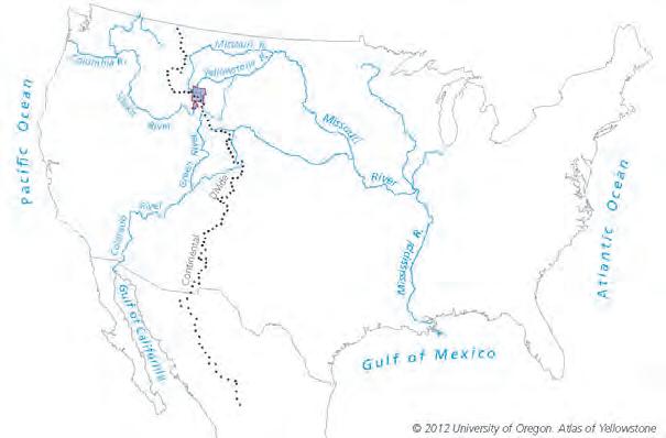
Figure 1-2. Two views—continental (inset) and regional—of major river systems that have headwaters in the Greater Yellowstone Area (GYA). (Image credits: Atlas of Yellowstone [Marcus et al. 2012]).

ThE huC6 WATERShEdS IN ThE GYA

In the 1980s, the United States Geological Survey (USGS) developed a hierarchical classification— the Hydrologic Unit Code (HUC) system—that subdivides the country’s river basins and watersheds into regions, subregions, and smaller units (Seaber et al. 1987; NRCS 2007; USGS undated). The HUC system divides land based on the physical properties of rivers and tributaries and is thus independent of political boundaries and ownership. We use the HUC system for the Greater Yellowstone Climate Assessment because the impact of climate change on GYA rivers can be better studied for individual watersheds than inside artificially defined borders (e.g., state or national park boundaries).

In the Assessment, we focus on six river basins that meet the definition of HUC level 6 (HUC6), also considered a subregion in USGS parlance. The area and elevation data in the following HUC descriptions are based on the 4-km (2.5-mi) resolution map shown in Figure 1-3:

о Missouri Headwaters (area: 6526 square miles [16,898 km2]; 21% of the GYA area) includes the Gallatin, Madison, Ruby and Upper Red Rock river watersheds. Elevation ranges from 4100-10,000 ft (1250-3050 m), with a mean elevation of 6900 ft (2100 m). The subregion supports the northern Centennial Range, the Ruby Range, the Madison Range, and the western side of the Gallatin Range. The city of Bozeman, and towns of Belgrade, Big Sky, and Ennis, Montana are in this HUC.

о The Upper Yellowstone (area: 7791 square miles [20,178 km2]; 23% of the GYA area) includes the Upper Yellowstone, which originates in Bridger-Teton National Forest, with the added tributaries of the Shields and Stillwater river watersheds. Elevation ranges from 4200-11,150 ft (1280-3400 m), with a mean elevation of 9850 ft (3000 m). The subregion includes the Absaroka Range, including the Beartooth Mountains, the Crazy Mountains, and the east side of the Gallatin Range and Bridger Range. The Montana towns of Livingston and Red Lodge are in this HUC.

о Big Horn (area: 5395 square miles [13,973 km2]; 10% of the GYA area) includes the Big Horn, North Platte, Clarks Fork, Shoshone, and Upper Wind river watersheds. Elevation ranges from 5250-12,139 ft (1600-3700 m), with a mean elevation of 8700 ft (2650 m). The region includes the Absaroka Range, the Owl Creek Range, and the north slope of the Wind River Range. Cody, Wyoming, is in this HUC, and Lander is near the border.

о Upper Green (area: 3486 square miles [9029 km2]; 17% of the GYA area) includes parts of the Upper Green, Upper Bear, Lower Bear, and the New Fork river watersheds. Elevation ranges from 6700-12,300 ft (2040-3750 m), with a mean elevation of 8400 ft (2560 m). The subregion extends from the south side of the Wind River Range to the Wyoming Range. Pinedale, Wyoming, is in this HUC.

о Snake Headwaters (area: 5772 square miles [14,591 km2]; 14% of the GYA area) includes the Upper Snake River, Gros ventre, Grays-Hoback, Salt, and Palisades river watersheds. Elevation ranges from 4840-9680 ft (1475-2950 m), with a mean of 6500 ft (1980 m). Jackson, Wyoming, is the largest community in this HUC. This region includes Grand Teton National Park, with the east side of the Teton Range, the Gros ventre Range, and Wyoming Range.

о Upper Snake (area: 4969 square miles [12,870 km2]; 16% of the GYA area) includes Henrys, Teton, and Upper Beaver-Camas river watersheds. Elevation ranges from 5250-10,732 ft (1600-3271 m), with a mean elevation of 7790 ft (2374 m). This is the lowest elevation HUC6 and includes the eastern end of the Snake River Plain. It is bound by the west side of the Teton Range and the south side of the Centennial Range. Driggs, Idaho, is in this HUC.

Most of our HUC6 watersheds include part of a main stem river (e.g., a segment of the Yellowstone River or Snake River) that is fed by smaller tributaries (designated as HUC8). In the case of the Snake Headwater and Upper Snake subregions, there is no single main stem river, but rather a set of intermediate-sized smaller rivers.

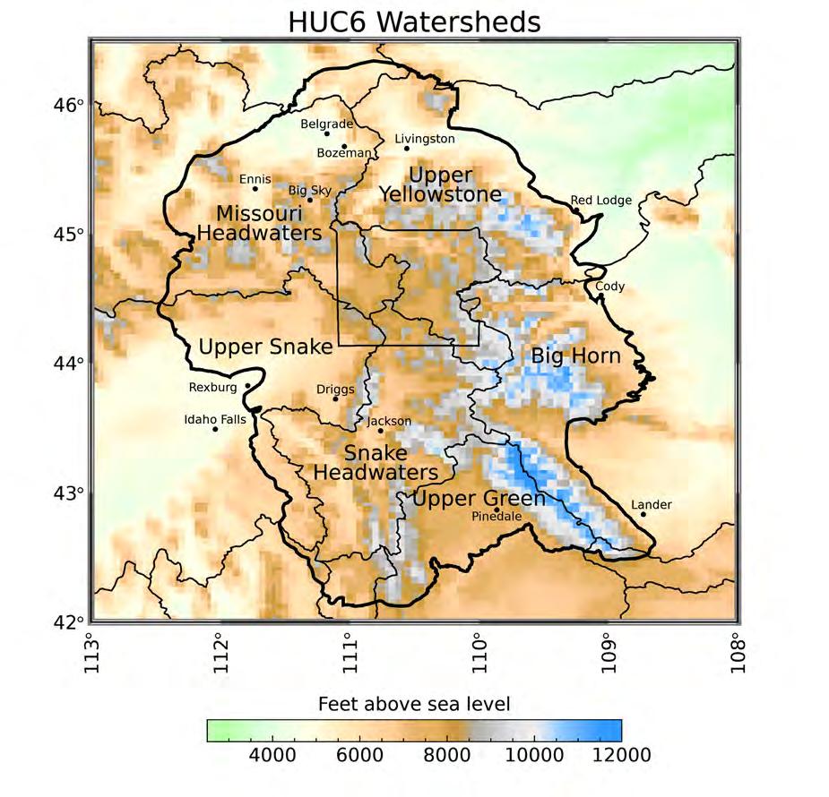
Figure 1-3. Topography of the Greater Yellowstone Area (GYA, dark outline). The names of the six Hydrologic Unit Code 6 (HUC6) watersheds addressed in this report are labeled. The topography is represented by 4-km (2.5-mile) grid cells, which is also the resolution of the climate and hydrology data in the report. Note that small areas of several other HUC6 watersheds are within the boundary of the GYA. For example, the Upper Missouri north of Belgrade MT and the Lower Bear south of the Snake Headwaters, and the North Platte south of Lander WY. For this study, we combined the smaller HUCs with the appropriate neighboring larger HUCs.

STRuCTuRE OF ThE ASSESSMENT

The Greater Yellowstone Climate Assessment—Past, Present, and Future Climate Change in Greater Yellowstone’s Watersheds is divided into nine chapters. Following this Introduction, in Chapter 2 we present basic concepts of climate and hydrologic change, summarize past climate changes in the GYA over the last 20,000 yr based on the geologic record, and explain the natural and anthropogenic drivers of climate change. In Chapter 3, we examine observed 20th- and early 21stcentury changes and trends in climate and water in the GYA based on weather and streamgaging station measurements. In Chapter 4, we provide an overview of the scientific methods used to develop projections of future changes in climate and water. In Chapters 5, 6, and 7, we present 21st-century projections of air temperature, precipitation, and water, respectively, with focuses on climate variables that are relevant to ecosystems, agriculture, winter recreation, and energy use. In Chapter 8, we offer some of the results of interviews with residents in the Greater Yellowstone Area, including their concerns for the future. In Chapter 9, we identify knowledge gaps and outline the next steps in the assessment process. The report also contains a glossary and several appendices that provide additional details for some chapters and include technical information about the data and methods used in the Assessment.

We begin Chapters 2, 3, 5, 6, 7, and 8 with key messages of the chapter’s information. These messages are accompanied by a statement of confidence by the chapter authors. Confidence levels are based on the authors’ judgment following the approach used by the Intergovernmental Panel on Climate Change’s (IPCC’s) Fifth Assessment Report (IPCC 2014). The greater the evidence, agreement, and statistical significance, the higher the level of author confidence in the certainty of the key message (Table 1-2).

Table 1-2. Chart of levels of agreement, evidence, and confidence in the key messages.

The authors of Chapters 2 rate their confidence in the observed data, with evidence of change as limited, medium, or robust, depending on the type, amount, and quality of the scientific information supporting the finding. These authors rate agreement as the consistency of the evidence (low, medium, or high) among scientific publications. The authors of Chapter 3 combine their confidence statement into a single net confidence rating.

In Chapters 5-7, the authors rate the confidence of projected climate and hydrologic changes from climate and water balance models. Consistent with the MCA (Whitlock et al. 2017), the authors report the number of models out of 20 that agree on the sign (positive or negative) of the median value of the future change. For example, if the median value is positive and 18 out of 20 models project positive change, then the percent agreement is 100 ×18/20 = 90%. In addition, the authors follow the IPCC (Meehl et al. 2007) and report the signal to noise ratios (SNRs). The SNR is the ratio of the mean change in a climate variable (signal) to the standard deviation of the 20 models comprising the mean (noise). SNRs greater than one (SNR >1) are used to establish when a projected climate change emerges over the 21st century (Hawkins and Sutton 2012) and provide additional support for confidence in the change. The categories for assigning model confidence are also based on guidance from the IPCC AR5 (Fifth IPCC Assessment Report) (Mastrandrea et al. 2010):

о high confidence—greater than 80% model agreement (more than 16 of the 20 models) with added confidence from SNR greater than 1;

о medium confidence—60 to 80% model agreement with or without SNR greater than 1;

о low confidence—less than 60% model agreement SNR less than 1.

These assignments of confidence on model-based results are specific to the projections in this Assessment.

Old homestead in the GYA

Photo courtesy of Cathy Whitlock

LITERATuRE CITEd

Al-Chokhachy R, Alder J, Hostetler S, Gresswell R, Shepard B. 2013. Thermal controls of Yellowstone cutthroat trout and invasive fishes under climate change. Global Change Biology 19:3069-81.

Bartlein PJ, Whitlock C, Shafer S. 1997. Future climate in the Yellowstone National Park region and its potential impact on vegetation. Conservation Biology 11:782-92.

Chang T, Hansen AJ. 2015. Historic and projected climate change in the greater Yellowstone ecosystem. Yellowstone Science 23(1):14-9.

Despain DG. 1990. Yellowstone vegetation: consequences of environment and history in a natural setting. New York NY: Roberts Rinehart. 239 p.

Hansen AJ, Phillips L. 2018. Trends for vital signs for Greater Yellowstone: application of a Wildland Health Index. Ecosphere 9:e02380.

Hawkins E, Sutton R. 2012. Time of emergence of climate signals. Geophysical Research Letters 39:L01702. doi:10.1029/2011GL050087.

[IPCC] Intergovernmental Panel on Climate Change. 2014. Climate Change 2014: synthesis report: contribution of working groups I, II and III to the Fifth Assessment Report of the Intergovernmental Panel on Climate Change. Pachauri RK, Meyer LA, eds. Geneva Switzerland: Intergovernmental Panel on Climate Change. 151 p.

[IPCC] International Panel on Climate Change. 2018. In: Masson-Delmotte v, Zhai P, Pörtner H-O, Roberts D, Skea J, Shukla PR, Pirani A, Moufouma-Okia W, Péan C, Pidcock R, Connors S, Matthews JBR, Chen Y, Zhou x, Gomis MI, Lonnoy E, Maycock T, Tignor M, Waterfield T, editors. Global Warming of 1.5°C: an IPCC Special Report on the impacts of global warming of 1.5°C above pre-industrial levels and related global greenhouse gas emission pathways, in the context of strengthening the global response to the threat of climate change, sustainable development, and efforts to eradicate poverty. 630 p. Available online https://www.ipcc.ch/site/assets/uploads/sites/2/2019/06/SR15_Full_Report_Low_Res.pdf. Accessed 8 Mar 2021.

Keiter RB , Boyce MS. 1991. The Greater Yellowstone Ecosystem, redefining America’s wilderness heritage. New Haven CT: Yale University Press. 428 p.

MacDonald D. 2012. Montana before history: 11,000 years of hunter-gatherers in the Rockies and Plains. Missoula MT: Mountain Press Publishing Company. 204 p.

Marcus WA, Meacham JE, Rodman AW, Steingisser AY. 2012. Atlas of Yellowstone. Berkeley CA: University of California Press. 274 p.

Marcus WA, Meacham JE, Rodman AW, Steingisser AY, Menke JT. 2022. Atlas of Yellowstone, 2nd edition. Berkeley CA: University of California Press. Forthcoming.

Mastrandrea MD, Field CB, Stocker TF, Edenhofer O, Ebi, KL, Frame DJ, Held H, Kriegler E, Mach KJ, Matschoss PR, Plattner G-K, Yohe GW, Zwiers FW. 2010 (Jul). Guidance note for lead authors of the IPCC Fifth Assessment Report on consistent treatment of uncertainties. Geneva: Intergovernmental Panel on Climate Change. 6 p. Available online https://www.ipcc.ch/site/assets/uploads/2017/08/AR5_Uncertainty_ Guidance_Note.pdf. Accessed 9 Mar 2021.

Meehl GA, Stocker TF, Collins WD, Friedlingstein P, Gaye AT, Gregory JM, Kitoh A, Knutti R, Murphy JM, Noda A, Raper SCB, Watterson IG, Weaver AJ, Zhao Z-C. 2007. Global climate projections [chapter 10]. In Solomon S, Qin D, Manning M, Chen Z, Marquis M, Averyt KB, Tignor M, MillerHL, eds. Climate Change 2007: The Physical Science Basis. Contribution of Working Group I to the Fourth Assessment Report of the Intergovernmental Panel on Climate Change. Cambridge UK and New York NY: Cambridge University Press. 1007 p.

Monahan WB, Fisichelli NA. 2014. Climate exposure of US national parks in a new era of change. PLOS ONE 9(7):e101302. doi:10.1371/journal.pone.0101302

[NPSa] National Park Service. [undated]. Greater Yellowstone Ecosystem [webpage]. Available online https:// www.nps.gov/yell/learn/nature/greater-yellowstone-ecosystem.htm. Accessed 26 Mar 2021.

[NPSb] National Park Service. [undated]. visitor use statistics. Available online https://irma.nps.gov/STATS/ SSRSReports/Park%20Specific%20Reports/Annual%20Park%20Recreation%20visitation%20(1904%20 -%20Last%20Calendar%20Year)?Park=YELL. Accessed 9 Mar 2021.

[NRCS] Natural Resources Conservation Service. 2007 (Jun). Watersheds, hydrologic units, hydrologic unit codes, watershed approach, and rapid watershed assessments [internal paper]. 2 p. Available online https://www.nrcs.usda.gov/Internet/FSE_DOCUMENTS/stelprdb1042207.pdf. Accessed 8 Mar 2021.

Pritchard JA. 1999. Preserving Yellowstone’s natural conditions: science and the perception of nature. Lincoln NB: University of Nebraska Press. 370 p.

Quammen D. 2016. A journey through America’s wild heart: Yellowstone. Washington DC: National Geographic Partners. 222 p.

Reese R. 1984. Greater Yellowstone, the national park and adjacent wildlands. Helena MT: Montana Geographic. 104 p.

Romme WH, Turner MG. 1991. Implications of global climate change for biogeographic patterns in the Greater Yellowstone Ecosystem. Conservation Biology 5:373-86. https://doi. org/10.1111/j.1523-1739.1991.tb00151.x.

Saunders S, Findlay D, Easely T, Christensen S. 2011 (Sep). Greater Yellowstone in peril; the threats of climate disruption [report]. Louisville CO and Bozeman MT: The Rocky Mountain Climate Organization and Greater Yellowstone Coalition. 55 p. Available online http://www.rockymountainclimate.org/images/ YellowstoneInPeril.pdf. Accessed 9 Mar 2021.

Schullery P. 1992. The Bears of Yellowstone. Worland WY: High Plains Publishing. 318 p.

Schullery P. 2004. Searching for Yellowstone: ecology and wonder in the last wilderness. Helena MT: Montana Historical Society Press . 352 p.

Seaber PR, Kapinos FP, Knapp GL. 1987. Hydrologic unit maps: US Geological Survey water-supply paper 2294. Denver CO: USGS. 66 p. Available online https://pubs.usgs.gov/wsp/wsp2294/pdf/wsp_2294.pdf. Accessed 8 Mar 2021.

[USCB] US Census Bureau. [undated]. National population totals and components of change 2010-2019; annual estimates of the resident population: April 1, 2010 to July 1, 2019. Available online. https://www. census.gov/data/tables/time-series/demo/popest/2010s-national-total.html. Accessed 9 Mar 2021.

[USCB] US Census Bureau. 2018 (Mar 22). New Census Bureau population estimates show Dallas-Fort Worth-Arlington has largest growth in the United States. Available online https://www.census.gov/ newsroom/press-releases/2018/popest-metro-county.html. Accessed 9 Mar 2021.

[USGCRP] US Global Change Research Program. 2017. Wuebbles DJ, Fahey DW, Hibbard KA, Dokken DJ, Steward BC, Maycock TK, editors. Climate science special report: fourth national climate assessment, vol 1. Washington DC: USGCRP. 470 p. doi:10.7930/J0J964J6.

[USGS] US Geological Survey. [undated]. Hydrologic unit maps [webpage]. Available online https://water. usgs.gov/GIS/huc.html. Accessed 28 Mar 2021.

Whitlock C. 1993. Postglacial vegetation and climate of Grand Teton and southern Yellowstone national parks. Ecological Monographs 63:173-98.

Whitlock C, Cross W, Maxwell B, Silverman N, Wade AA. 2017. 2017 Montana Climate Assessment. Bozeman and Missoula MT: Montana State University and University of Montana, Montana Institute on Ecosystems. 318 p. doi:10.15788/m2ww8w.

Bridger Foothills Fire near Bozeman MT, September 2020

Photo courtesy of Janice Gaedtke

2. CLIMATE, CLIMATE VARIABILITY, AND CLIMATE CHANGE IN THE GREATER YELLOWSTONE AREA

Cathy Whitlock, Steven Hostetler, Gregory Pederson, and David Liefert

kEY MESSAGES

о The climate history of the Greater Yellowstone Area shows changes on timescales ranging from seasons to millennia. Over thousands of years, the primary drivers of natural climate change are cyclical variations in solar radiation related to Earth’s orbit around the sun and associated changes in the amount of greenhouse gas in the atmosphere. Over years to centuries, the natural drivers of climate variability are volcanic activity, solar output, and coupled atmosphere-ocean circulation patterns. [high agreement, robust evidence]

о The geologic record of the GYA indicates that the last glaciation (approximately 22,00013,000 yr ago) was as much as 5-7°F (2.8-3.9°C) colder than the pre-industrial period (1850-1900). Two warm periods in the past are the early Holocene (11,500-7000 yr ago), which was about 1.8-3.6°F (1-2°C) warmer in summer than the pre-industrial period, and the Medieval Climate Anomaly (from 800 to 1300), characterized by prolonged droughts and slightly warmer summers than pre-industrial time. [high agreement, robust evidence]

о The average temperature of the last two decades (2001-2020) is probably as high or higher than any period in the last 20,000 yr, and likely higher than previous glacial and interglacial periods in the last 800,000 yr. The current level of carbon dioxide in the atmosphere is the highest in the last 3.3 million years. [medium agreement, medium evidence]

WhAT IS CLIMATE?

Climate differs from weather. Weather refers to atmospheric changes that occur over minutes to months and are reflected, for example, by the temperature, humidity, and precipitation at a location and particular time. Climate is the long-term average of weather over an extended time period, such as decades to centuries. In this report, we define the climate base period for comparison with future periods as the 1986 through 2005 average or mean. We chose this 20year base period because 1) it captures observed global warming trends and, therefore, is a conservative (warm) baseline; and 2) climate model simulations of the historical period end in 2005 and projections of future climate in this Assessment begin in 2006.

The climate system describes all the interacting components that create Earth’s climate: the atmosphere (air), hydrosphere (water), the cryosphere (ice and permafrost), lithosphere (Earth’s upper rocky layer), and biosphere (living things). Climate change refers to shifts (e.g., decadal and longer) in the average or mean climate, which can be abrupt or gradual, as evidenced in historical and geological records discussed later in this chapter and in Chapter 3. A climate trend is a longterm trajectory of change in the mean climate. Climate variability refers to short-term departures from the mean state of the climate (note that climate variations are longer than individual weather events, spanning seasons or years). In the coming decades, climate change is projected to trend toward ever warmer conditions; however, as illustrated in Figure 2-1, climate variability may result in seasons and years that are warmer or colder than the 20-year means, just as occurs today.

Figure 2-1. An example of climate change that displays both trend and variability. The black line shows steadily increasing temperature through time with year-to-year temperature variations along with a linear trend shown by the gray line. The three horizontal lines indicate the average or mean temperature for three 20-year periods, as examples of the averaging periods used in the Assessment, and the shading shows the range of temperature variability (minimum to maximum) during each averaging period.

CLIMATE ANd WATER vARIAbLES dISCuSSEd IN ThE ASSESSMENT

The international climate science community uses over 50 essential physical, chemical, and biological variables to characterize the state of the Earth’s climate (WMOa undated). To qualify as an essential climate variable, the information about it must be 1) worldwide in coverage; 2) freely available; 3) quality controlled with appropriate documentation; and 4) considered relevant by an international panel of climate experts. Our report focuses on a small subset of the 50 essential climate variables that are relevant to the GYA:

о Air temperature (referred to temperature in this report) is a measure of how hot or cold the air is with reference to some standard value. Seasonal variations in temperature result from latitudinal differences in the amount of solar radiation received at the Earth’s surface, contrasts in seasonal heating of land and oceans, and atmospheric circulation.

о Precipitation is the quantity of water (liquid or solid) falling to the Earth’s surface at a specific place over a given period. Like temperature, precipitation varies from season to season and place to place and depends on coupled atmospheric-ocean circulation.

In addition to the climate variables, we also focus on other variables:

о Snowfall and snowpack are measures of the amount and fate of solid winter precipitation. Snowfall is the amount of accumulated snow after a storm. It is measured in terms of the depth of solid water it contains. In mountainous and relatively dry areas like the GYA, 10 inches (25 cm) or more of snow is often needed to create 1 inch (2.5 cm) of liquid water when melted. Snowpack is the amount of snowfall that accumulates over the cold season. It also is measured by both depth (snow depth) and the amount of liquid water it stores (called snow water equivalent or SWE).

о Streamflow (also called discharge) refers to water moving within a river measured by the volume of water passing a point in a given time. Streamflow is measured at gaging stations in units of cubic feet per second or cubic meters per second. In GYA, streamflow is strongly controlled by the seasonality of runoff from snowmelt.

о Runoff is the depth of water uniformly distributed over an area, such as a watershed. It is the potential amount of water available for groundwater and streamflow.

о Evapotranspiration is water lost through evaporation from bare soil and transpiration by plants. Potential evapotranspiration is the amount of evapotranspiration that would occur under unlimited water availability.

о Drought is a prolonged period of dryness relative to long-term average conditions. The climatological community defines four types of drought: 1) meteorological drought occurs when unusually dry weather patterns persist over an area from days to months; 2) hydrological drought refers to low-water supply and usually occurs after many months of meteorological drought; 3) agricultural drought occurs when

low soil moisture limits survival and production of crops and grazing lands; and 4) socioeconomic drought reflects the economic and social impact of a combination of hydrological and agricultural drought. In this report, we use the term drought, without distinguishing the type, but unless otherwise noted, we are referring to meteorological or hydrological drought.

о Palmer Drought Severity Index (PDSI) is a standard measure of drought that combines temperature or potential evapotranspiration and precipitation data to quantify dryness or wetness relative to average or normal conditions. The PDSI describes soil moisture conditions (generally the top meter of soil).

о Vapor pressure deficit is a measure of the drying capacity of the atmosphere based on air temperature and relative humidity. High vapor pressure deficits (i.e., high temperature combined with low humidity) can limit tree growth, increase their vulnerability to drought, and dry fuels, all potential contributors to wildfire.

pRESENT CLIMATE

The climate of the GYA is characterized by long, often bitterly cold winters. Summers are short and mild. May and June are generally the wettest months in the valleys; August is generally the driest. Snow is the primary form of winter precipitation.

The GYA’s climate is attributed primarily to its mid-latitude continental location, high average elevation, and distance from the Pacific and Gulf coasts. At approximately 44oN latitude, the region has long summer days and long winter nights. Even summer days are relatively cool, however, due to the high elevation of the GYA. GYA receives air masses not only from the Pacific Ocean to the west, but also from the Arctic Ocean to the north and Gulf of Mexico to the south. The relative contribution of these air masses and the moisture they entrain is reflected in seasonal temperature and precipitation patterns for any given year (Whitlock and Bartlein 1993).

Precipitation generally increases with elevation in GYA, as it does throughout the West. Cold, wet winters in the GYA reflect a combination of moisture carried by storms off the Pacific Ocean and frequent, cold Arctic air mass intrusions. Most of these storms are funneled northeastward along the Snake River Plain and the precipitation they carry is delivered as snow over the high mountains and plateaus of the GYA (Farnes 1997). Cold, dry weather in winter occurs when a sustained southward incursion of an Arctic air mass brings subzero temperatures (Fahrenheit) to the region. Winters are generally wetter in the Teton Range and western Yellowstone Plateau region than in the eastern GYA. Pacific storm systems, as well as moisture transported along the Rocky Mountain Front from the Gulf of Mexico, account for wet spring conditions in the region.

Summers in much of the GYA are typified by warm, dry conditions punctuated by thunderstorms. During summer, Pacific storm tracks shift well north of the GYA so summer rainfall is delivered by low-pressure centers and their related atmospheric disturbances (or fronts). Moisture in the northern and eastern GYA originates from the subtropical Gulf of Mexico, whereas that in the southwestern GYA comes from the subtropical Pacific Ocean.

Year-to-year and decadal climate variations that affect the GYA derive from recurring, global scale changes in atmosphere and ocean circulation patterns. The El Niño-Southern Oscillation (ENSO), for example, is a climate pattern set up by changes in sea-surface temperature and atmospheric pressure in the equatorial Pacific Ocean that can persist for several years. Warmer-than-normal equatorial ocean surface temperatures are associated with El Niño events, whereas colder surface temperatures are associated with La Niña events. ENSO influences storm tracks and pressure systems at mid-latitudes through atmospheric connections (called teleconnections) that, in turn, influence surface climate conditions across the West, including the GYA (Figure 2-2). The Pacific Decadal Oscillation (PDO) is a similar, multi-year pattern of climate variability forced by seasurface temperature changes that occur on decadal scales. Phases of the PDO are identified by warm or cold ocean temperature patterns in the north Pacific Ocean. Even persistent decades of warmer and colder than normal sea surface temperature in the North Atlantic Ocean known as the Atlantic Multi-decadal Oscillation (AMO) can interact with ENSO and PDO to affect long-term drought in the GYA (McCabe et al. 2004, 2008).

Figure 2-2. Differences or anomalies from mean annual temperature (top row) and precipitation (bottom row) from 1950-2010 during El Niño (left column) and La Niña (right column) (figure from Kennedy 2012). El Niño events tend to bring warmer and drier conditions than average to the Greater Yellowstone Area (GYA), whereas La Niña events tend to bring cooler and wetter conditions, especially in the western GYA. El Niño-Southern Oscillation (ENSO) patterns are unstable spatially and through time as a result of interactions with other atmosphere-ocean processes. A particular ENSO event does not always result in the same surface climate conditions in the GYA.

ENSO and PDO patterns alter the north-south position of Pacific storm tracks across western North America, which can result in large and contrasting variations in winter precipitation and air temperature that persist for short (~12-18 months) to long (decades) periods. The regional effects on precipitation from changes in the PDO are strongest along the Pacific Coast in the Pacific Northwest, whereas the greatest influence of ENSO is over the American Southwest and Southeast. On average, El Niño events bring warmer and drier conditions to the GYA whereas La Niña events bring cooler and wetter conditions; however, interaction with other atmosphereocean circulation processes often affect this generalized pattern. Thus, not all ENSO or PDO events have a similar effect on the climate of the GYA (Pederson et al. 2011a,b; Abatzoglou 2011; Pederson et al. 2013).

pAST CLIMATE ChANGE

Natural climate change, ever ongoing, can be examined on many timescales. Over millions to 100s of millions of years, changes in the size and position of continents and ocean basins and related mountain uplift have shaped the Earth’s climate. Over tens to hundreds of thousands of years, repeated cycles of cold (called glacial periods or ice ages) and warmth (called interglacial periods) have been caused by seasonal and latitudinal variations in the amount of solar radiation received by the Earth.

Glacial-interglacial cycles result from continual changes in the tilt and wobble of Earth’s axis and in the elliptical orbit of the Earth around the sun. These recurring astronomical drivers1 of climate change, known as Milankovitch cycles, are the pacemaker of the ice ages (Ruddiman 2013). Levels of greenhouse gases in the atmosphere also varied with these cycles, amplifying the warmth of interglacial periods and the cold conditions of glacial intervals. The last ice age on the planet occurred between about 115,000 and 11,700 yr ago, with maximum glaciation between 27,000 and 19,000 yr ago in different regions (Clark et al. 2009). Global warming of 5-7°F (3-4°C) occurred between 19,000-11,000 yr ago, ushering in the current interglacial period, which is called the Holocene (the last 11,700 yr) (Clark et al. 2012; IPCC 2013).

Climate variations on timescales of centuries or less tend to be more regional in scale, but with different principal drivers (Ruddiman 2013):

о Over decades to centuries, volcanic activity, changes in solar output, and globalscale changes in atmosphere-ocean circulation patterns have caused climate to vary. Notable examples of such variations have resulted in climate anomalies relative to a defined average, such as the persistent cold conditions and widespread glacial advances that occurred from about 1600-1850, known as the Little Ice Age, and the periods of warmth and drought that define the Medieval Climate Anomaly from about 800-1300.

о Over interannual to decadal timescales, persistent atmosphere-ocean circulation patterns, such as ENSO and the PDO, are the important drivers of climate variations (discussed above).

1 Some authors use the word forcings instead of drivers. For this report we will generally use the latter.

The last 20,000 years

The climate of the GYA has varied widely over the last 20,000 yr—from the culmination of an ice age to periods that were warmer than the pre-industrial period2. The climate history of the GYA, as interpreted from the geologic record and measured by observations, provides a useful context for perspective on the significance of current and projected climate changes.

GYA was extensively covered by ice during past glacial periods. Ice cover during the recent Pinedale glaciation (22,000-13,000 yr ago) and the previous Bull Lake glaciation (150,000-140,000 yr ago) are shown in Figure 2-3 (Licciardi and Pierce 2018). The Pinedale glaciation began when glaciers started to grow and expand in the Beartooth-Absaroka Mountains of northeastern GYA and Gallatin Range of northwestern GYA. By 15,000 yr ago, individual glaciers from the two regions had coalesced into a large Yellowstone ice cap centered over present-day Yellowstone Lake. valley glaciers flowed from the ice cap down all the major river valleys. Geologists name the terminal ridges of gravel and boulders (moraines) deposited by these valley glaciers by their location (e.g., the Chico moraine, the Outer Jenny Lake moraine) and determine the age of the moraines using cosmogenic nuclide dating methods3. From this information, geologists have determined that Yellowstone ice cap was asymmetrical; its maximum growth occurred to the southwest, indicative of the dominant source of precipitation from the direction of the Snake River Plain (Licciardi and Pierce 2018). Glaciers started to recede first in the northeast in the Clarks Fork drainage 19,800 yr ago, and last in the south at Jackson Lake 15,500 yr ago. Glacial ice was largely gone from the GYA by 12,000 yr ago.

2 Pre-industrial refers to the period when fossil-fuel burning had yet to change the climate. This period (18501900) is used as baseline for assessing current climate change (IPCC 2018).

3 Cosmogenic nuclide dating uses the interactions between cosmic rays and the atomic nuclides found in glacially transported boulders to provide age estimates for the rock’s exposure at the Earth’s surface (Davies 2020). In other words, cosmogenic nuclide dating determines how long the boulders in moraines have been at the surface, which in turn provides the age of glacier position.

Yellowstone Lake was once covered by an ice cap

Photo courtesy of Cathy Whitlock

Figure 2-3. Extent of ice cover during the Pinedale (22,000-13,000 yr ago) and previous Bull Lake glaciations in the Greater Yellowstone Area (GYA) (image from Licciardi and Pierce [2018]; reprinted with permission). Pinedale-age glaciers were larger than those of Bull Lake in the northern and eastern parts of GYA, and smaller in the southern and western parts. Ages, shown in thousands of years ago (kiloannum = ka), of the glacier limits are based on cosmogenic exposure dating of moraine boulders. Contours (purple lines) show the elevation of the ice cap surface in thousands of feet. The three circles provide ages (ka) and locations of the highest ice elevation at 15,000, 18,000, and 20,000 yr ago. Note the southwesterly advance of the ice cap with time.

The present-day landscape, river systems, and lakes of the GYA were formed largely during the Pinedale glaciation by the erosional and depositional processes associated with ice advance, melting, and recession (Good and Pierce 1996). The ruggedness of Teton and Wind River ranges exemplify glacial sculpting under former ice divides (Figure 2-4). The sagebrush-covered terraces within the major river valleys were created by high-volume braided rivers that flowed from melting glaciers and deposited coarse gravels beyond the ice margins. These porous gravels are the source of shallow, groundwater storage in most of the GYA’s river basins. Many lakes in the GYA (e.g., Jenny Lake, Jackson Lake, Fremont Lake) are dammed by moraines of gravel that were deposited at the terminus of valley glaciers. Other smaller lakes (e.g., Blacktail Pond, Swan Lake, Swamp Lake) were formed when blocks of ice buried under glacial debris melted with warming temperatures and created a depression on the land surface.

Figure 2-4. This iconic photo by Ansel Adams shows the legacy of past glaciation in Grand Teton National Park (1942). About 16,000 yr ago, the southern margin of the Yellowstone ice cap reached the valley of Jackson Hole. As the climate warmed about 15,500 yr ago, the position of the southern ice margin retreated northward (to the right in the photo). In the process of ice melting, an ancient, braided Snake River flowed from the glacial terminus and deposited a sheet of gravel and cobbles on the valley floor. These gravel deposits formed flat terraces that are today covered by sagebrush (middle distance). The Snake River continues to carve through these glacial deposits in a meandering pattern, creating gravel bars covered with cottonwoods (foreground). The Teton Range (background) was carved by their own set of glaciers; the small glaciers in the Teton Range today are remnants of more extensive ice cover. (Photo credit: US National Archives Identifier 519905.)

As the climate warmed and glaciers started to melt in the GYA, plants were able to colonize areas that had previously been covered by ice. Pollen buried in the sediment in Yellowstone’s lakes indicates that the first conifer to appear was juniper, probably common juniper (Juniperus communis), which established in a relatively open, tundra-like landscape. Next came Engelmann spruce (Picea engelmannii), followed by whitebark pine (Pinus albicaulis), limber pine (Pinus flexilis), and subalpine fir (Abies lasiocarpa) (Krause and Whitlock 2017). Lodgepole pine (Pinus contorta) was widespread after 11,000 yr ago, and Douglas-fir (Pseudotsuga menziesii) was the last conifer to arrive and expand its range after 9000 yr ago (Iglesias et al. 2018).

This sequence of forest development shows the capacity of the region’s conifers to respond to rising temperatures by adjusting their range and abundance over thousands of years. Similar responses will certainly take place in the future, but likely at a faster rate. Some native species (e.g., whitebark pine) may no longer find suitable climate in GYA and become regionally absent (Chang et al. 2014) and different species (e.g., Gambels oak [Quercus gambelii], western larch [Larix occidentalis], ponderosa pine [Pinus ponderosa]) may be better suited to future climate conditions. The rate of current climate change, however, is many times faster than what occurred in the past, and it is doubtful that species will be able to keep pace on a timescale relevant to forest management (Bartlein et al. 1997).

The current interglacial period, the Holocene, began as the latest of a series of interglacial periods. Two warm intervals in the Holocene serve as important benchmarks for evaluating future climate and ecological change in the GYA (Whitlock and Hostetler 2019). The first was a prolonged period from about 11,500 to 7000 yr ago (the early-Holocene period) when summers in the region were on average 1.8-3.6°F (1-2°C) warmer than the pre-industrial average (Kutzbach et al. 1998: Bartlein et al. 1998). The causes of this warming were increased solar radiation during the Northern Hemisphere summer resulting from slow Milankovitch variations in the tilt of the Earth’s axis and rising levels of greenhouse gases in the atmosphere.4

Pollen records indicate that the early-Holocene period in the GYA was a time of expanded lodgepole pine forest and more Douglas-fir and aspen (Populus tremuloides) compared to present. The upper tree line lay at a higher elevation than at present in response to longer growing seasons, and lower tree line shifted upslope in response to drought (Whitlock 1993; Iglesias et al. 2018). Many of the small lakes and wetlands in northern Yellowstone National Park dried during the early Holocene, and fires were more frequent. Snow and ice fields at high elevations shrank in size and accumulated plant debris and artifacts that were preserved by ice during subsequent cold periods (see box). Longer summers at Yellowstone Lake likely resulted in earlier ice-off in spring and longer open-water conditions in fall (Thompson et al. 1998).

4 Winter insolation was lower in the early Holocene and as a result winters in the GYA were probably cooler than during pre-industrial time.

Snow and Icefields of the Greater Yellowstone Area

Patches of year-round ice are found at high elevations throughout the Greater Yellowstone Area (GYA), and scientists have discovered that some of these patches are thousands of years old and preserve valuable information about the past. Recent warming has resulted in substantial melting and shrinking of the ice bodies, exposing organic artifacts that have been frozen in the ice. GYA artifacts provide unique insights into the activities of ancient hunter-gatherers in the high mountains. For example, a 10,300-year-old atlatl dart, used in hunting big game, was recovered from a melting ice patch in northwestern Wyoming (photos).

These ice patches are also a valuable source of paleoenvironmental and paleoclimatic information (Chellman et al. 2021). In 2018, a 6-m-long ice core was taken from the same ice patch where the atlatl dart shaft was found. The core contained 29 layers of plant remains (e.g., seeds, pollen, needles, and organic matter), animal dung, and dust (photo). Radiocarbon dating revealed that these debris layers formed during periods of warm and/or dry conditions that occurred on average every 300 yr over the last 10,000 yr.

A nearby melting ice patch uncovered fossil logs of whitebark pine (Pinus albicaulis), indicating that during a warm period 5000 yr ago conifers grew at elevations at least 100 m (330 ft) above presentday tree line. Tree-ring analysis of the wood showed that this warm period persisted for about 800 yr. Scientists expect more discoveries as a warming climate continues to melt old ice patches. Uncovered debris and artifacts will help us better understand past high-elevation environments, as well as the people who lived there.

Top: This 10,300-year-old atlatl foreshaft from the GYA is the oldest organic artifact recovered from an ice patch anywhere in the world.

Bottom: Detail of foreshaft showing three parallel ownership marks (red arrow) near where the projectile point would have been attached. (Photo credits: by Craig Lee)

Left: Scientists taking an ice core from a GYA ice patch.

Right: Sampling logs from ancient whitebark pines that have been exposed from a melting ice patch. (Photo credits: Greg Pederson)

The last 1000 years

The second period of warmth since the last ice age, the Medieval Climate Anomaly (800-1300), occurred on most continents, although the underlying cause of warming is not fully understood. Tree-ring records and other studies from GYA offer regional information about past temperature, precipitation, summer drought, snowpack, and streamflow over the last 1000 yr. The Medieval Climate Anomaly was overall not as warm as the early Holocene and instead was characterized by multi-decadal periods of warm summer temperatures, low snowpack, and dry conditions, which are referred to as megadroughts (Pederson et al. 2011b; Martin et al. 2019; Heeter et al. 2021).

Megadroughts occurred in the GYA and across much of the western United States in the early 600s, late 800s, 1200s, and late 1500s (Williams et al. 2020). These dry periods led to more fires, desiccation of small lakes, reduced streamflow, an upslope shift in upper tree line, and reduced Old Faithful geyser activity (see box) (Meyer et al. 1995; Millspaugh et al. 2004; Pederson et al. 2011b; Hurwitz et al. 2020).

Severe 13th-century Drought Silences Old Faithful

Old Faithful Geyser got its name in the 19th century because its eruptions were both regular and predictable. Recent years of low precipitation have resulted in less frequent eruptions of Old Faithful, and this slowdown has raised concerns from the public.

To investigate this change in eruption frequency, a team of scientists were given permission by Yellowstone National Park to collect 13 mineralized specimens of lodgepole pine (Pinus contorta) wood from the Old Faithful geyser mound (Hurwitz et al. 2020). The fact that trees at one time grew on the mound suggests that the geyser was not actively erupting at some point in the past. When eruptions at Old Faithful resumed, the trees were killed and preserved in mineral deposits. Radiocarbon dating of the wood samples show that tree establishment and associated eruption hiatus occurred in the early-13th through mid-14th centuries (1233-1362).

Independent climate studies based on tree-ring records indicate a severe and sustained drought across GYA in the mid-13th century at the time the trees grew on the Old Faithful mound. The scientists hypothesize that reduced precipitation limited the subsurface supply of water to the geyser basin causing a cessation in eruptions of Old Faithful for an extended period of time.

Old Faithful Geyser in Upper Geyser Basin, probably taken in 1878.

(Photo credit: William Henry Jackson, USGS, public domain)

The Medieval Climate Anomaly was followed by a period of above-average snowpack, renewed glacial activity, and cool conditions called the Little Ice Age. The Little Ice Age occurred at different times around the world, and its beginning and end are variously defined (Mann 2003; Neukom et al. 2019). In this Assessment we use the period from about 1550-1850, but note that cooling events began as early as 1300 in the GYA (Heeter et al. 2021). Cooling during the Little Ice Age may have been triggered by heightened volcanic activity, decreased solar activity, a shift in atmosphereocean circulation patterns, or even increased forest cover (acting as a carbon sink) during times of human population decline (Mann 2003; Ruddiman 2013). Glaciers at high elevations in the Rocky Mountains were reactivated during this period (Carrara et al. 1987; Menounos et al. 2009), and annual snowpack was high in the GYA during the years of 1535-1550, 1600-1620, 1660-1790, and 1845-1895 (Pederson et al. 2011b). Following the Little Ice Age, the lowest snowpack of the last 1000 yr occurred from 1900 to 1949 and since the 1980s (see box).

Changing Snowpack in the Greater Yellowstone Area

The steady decline in snowpack since the 1980s (measured as the amount of liquid water [or snow water equivalent] on April 1) is a concern for natural resource managers and communities that depend on mountain snowpack for their water supply.

While the great ecological and societal importance of mountain snowpack is clear, the observational record of mountain snowpack variability is short. Thus, scientists used records of tree growth that are sensitive to changes in snowpack across the GYA to reconstruct April 1 snow water equivalent for over the past 800 yr (Pederson et al. 2011b).

The reconstruction (see figure) shows a significant decrease in snowpack during the 20th and early 21st centuries as compared to the previous 800 yr. During the Little Ice Age (circa 1550-1850; shown in blue shading), glaciers in GYA, like elsewhere in the northern Rocky Mountains, reached their greatest extent of the Holocene as a result of persistent above average snowpack and cool summers. Conversely, exceptionally low snowpack during the 1930s Dust Bowl drought (shown in red shading) and since the 1980s—both attributed in part to warm summer conditions— has not been observed since at least the Medieval Climate Anomaly (800-1300).

Tree-ring reconstructions of the amount of water stored in April 1 snowpack across the Greater Yellowstone Area (GYA). Annual departures in April 1 snow water equivalent (SWE) from the 12502000 average (horizontal line) are based on information from tree-ring records (gray line) and recent observations (black line). Annual changes in the data are highlighted by the thin blue line and decadal trends are highlighted by the thick dark blue line. The Little Ice Age (mid-1500s to mid-1800s) is shown by the blue shading; the 1930s Dust Bowl drought is indicated by the pink shading. The observed data for the late 20th and early 21st century come from long-term NRCS snow course and SNOTEL (snow telemetry) records.

The tree-ring based reconstructions of snowpack in the GYA indicate that variations in summer temperature govern the overall amount of snowpack that persists over the long term (decades to centuries), whereas short-term differences (year-to-year to decadal) in snowpack are caused by variability in precipitation. The snowpack reconstruction implies that the recent decades of extremely low April 1 snow water equivalent relative to the last 800 yr are associated with regional warming; warming in the future will likely continue this trend (as discussed in Chapter 6).

The tree-ring based reconstructions of snowpack in the GYA indicate that variations in summer temperature govern the overall amount of snowpack that persists over the long term (decades to centuries), whereas short-term differences (year-to-year to decadal) in snowpack are caused by variability in precipitation.

The last 120 years

Observations over the last 120 yr (1900 to present) show long-term trends in temperature and precipitation with substantial year-to-year and decadal variability, including extreme dry and wet episodes relative to average conditions (Figure 2-5C). Some notable events in the GYA associated with trends and variability over the last 120 yr include:

о Trends across the 120-year period.—Mean annual temperature and precipitation in the GYA have varied over the last 120 yr with a substantial range of year-to-year variability and extended periods that were drier or wetter and colder or warmer than average (Figures 2-5A and B). After an extended dry period from 1905-1945 that included the 1930s Dust Bowl drought, precipitation has been near or above the longterm average. GYA temperatures were below the long-term average before late 1920s and then increased during the Dust Bowl years. Temperatures then dropped to near average values until the late 1970s, when they started to increase substantially. The combination of changing temperature and precipitation resulted in variable drought conditions as characterized by the Palmer Drought Severity Index (PDSI). The PDSI shows a few extreme droughts in the past 120 yr, such as in the 1930s, 1988, and early 2000s (Figure 2-5C). Extreme cold and heavy snow events that were common in the late 19th century are now rare (see box).

о Decadal-scale variability: the 1930s Dust Bowl drought.—Moisture variability across the GYA is evident as wet and dry conditions that lasted for decades (highlighted by 20year smoothing average in Figure 2-5A and C). The tendency for moisture conditions to persist over extended periods presents unique challenges for resource managers and local communities. For example, sustained low precipitation, elevated temperatures, and drought conditions during the 1930s Dust Bowl event (orange highlighted boxes in Figure 2-5) resulted in years of elevated regional fire activity, severely reduced surface water resources and streamflow, and the foreclosure and sale of many farms and ranches around the GYA (Murphy 2003). In many USGS streamgage records in the GYA, the Dust Bowl drought still ranks as one of the most severe and sustained drought events on record.

о

Year-to-year variability: the 1988 Yellowstone National Park fires.—Unusually little precipitation fell in 1988 (red point, Figure 2-5A), when extensive forest fires swept through Yellowstone National Park. Average temperature was high and precipitation was low in 1988 (Figure 2-5B) resulting in severe drought, as indicated by the Palmer Drought Severity Index (PDSI; Figure 2-5C). PDSI is a measure of drought intensity that accounts for both the current weather and the cumulative effects of precipitation and temperature from previous months. (See the wildfire box in Chapter 3 for more information.)

Classification of Palmer Drought Severity Indices

0.49 to -0.49 near normal

-0.5 to -0.99 incipient dry spell

-1.0 to -1.99 mild drought

-2.0 to -2.99 moderate drought

-3.0 to -3.99 severe drought

-4.0 or less extreme drought

Figure 2-5. Climate trends and variability for the last 120 yr in the Greater Yellowstone Area (GYA). Mean annual precipitation (A), mean annual temperature (B), and the Palmer Drought Severity Index (C; PDSI). The black lines in panels A and B are mean annual precipitation and temperature, respectively. The blue lines are 20-year smoothed averages of the annual values; the horizontal line is the 1905-2018 mean for precipitation (A) and temperature (B), and the 1900-1920 zero line for PDSI (C). The PDSI in panel C is a measure of long-term wetness (positive values) and dryness (negative values). Values of the PDSI range from +4 to -4 (see table above for categories). The red dots indicate the warm, dry conditions of 1988 and the orange shading marks the Dust Bowl years of the 1930s. Temperature and precipitation are the average of all 4-km (2.5 mile) grid PRISM points in the GYA (PRISM Climate Group 2020), and PDSI data are from NOAA National Centers for Environmental Information (NOAAa undated).

The Children’s Blizzard of 1888 and Bygone Cold Events

Naomi Schadt, Montana State University, and Cary J Mock, University of South Carolina

A century before the Yellowstone fires of 1988, an extreme natural disturbance of a different type occurred: the Children’s Blizzard of 1888. The morning of January 12, 1888, was warm and calm across GYA and onto the Great Plains, but these conditions abruptly changed as an Arctic cold air mass enveloped the region, causing temperatures to plummet to subzero values. Children were making their normal trek to rural schools, but when the icy weather hit en route, some attempted to return home. Many didn’t make it back to their families and perished while stranded in the storm (Potter 2012). It is estimated that 250-500 individuals died in this event (valle undated).

The Children’s Blizzard of 1888 was one of a series of severe, cold winter storms that swept the United States—from the Rocky Mountains to the East Coast—during the late 1800s and early 1900s. These winter storms were usually preceded by relatively warm weather and characterized by sudden drops in temperature and heavy snow.

Records from Camp Sheridan (now Mammoth) in Yellowstone National Park reported severe cold snaps and heavy snow starting January 3rd and extending to January 20, 1888, the year of the Children’s Blizzard. The lowest temperature recorded was -41°F (-40.5°C) on January 14, 1888. The high temperature on that same day was -25°F (-32°C). During that month, the Camp recorded almost 30 inches (76 cm) of snow. Thirteen out of those 17 snow days experienced lows below -20°F (-29°C) (US National Archives and Records Administration undated).

The previous year, 1887, Montana ranchers experienced high cattle losses in what is now known as “The Great Die-Up.” Heavy snows, low temperatures, and strong winds created a thick crust of ice and snow that livestock could not break through to reach the sparse grasses beneath. Lack of food and exposure to the elements proved disastrous for Montana cattle (LeCain 2017).

Today, subzero cold weather is often associated with cold Arctic air and little snow. National Weather Service data from Bozeman, Montana, and Cody, Jackson, and Mammoth, Wyoming, show periods of extended subzero cold in the last 50 yr, but typically these periods received less than 5 inches (13 cm) of snow. At these four stations, 6 days in the last half century registered temperatures below -40°F (-40°C; the low recorded during the Children’s Blizzard of 1888). All 6 days occurred in Jackson WY (Climate Analyzer undated).

In the last decade (2010-2019), there have been only five times in the GYA when 8 inches (20 cm) or more of snow accumulated in a 48-hour period that also featured subzero drops in temperature. Four of these weather events occurred in Mammoth WY (in 2010, 2014, 2017, and 2019) with the lowest temperature of -29°F (-34°C) during the 2019 storm. The low temperature recorded in Bozeman MT during this same storm was -10°F (-23°C).

No GYA weather event in the last decade measures up to the 7 days of negative temperatures and 30 inches (76 cm) of snow that was recorded between the 3rd and 20th of January 1888. Our winters have gotten warmer and the absence of the extreme, extended sub-zero periods is an indication that the climate of GYA is changing.

An image in Frank Leslie’s Weekly (1888) of the Children’s Blizzard in the Dakotas

CAuSES OF CLIMATE ChANGE

The Earth’s energy balance is driven by solar radiation that is absorbed by land surface and oceans and radiated back to the atmosphere as heat (Figure 2-6). Greenhouse gas (GHG) molecules, like water vapor (H2O) and carbon dioxide (CO2), have chemical bond structures that trap some of the heat from the Earth’s surface that otherwise would escape back to space. In this way, GHGs promote the accumulation of heat in the lower atmosphere that is necessary to sustain life. (Without atmospheric water vapor and GHGs, the global temperature would be -0.4°F [-18°C], roughly 59°F [33°C] colder than present [WMOb undated].)

The heat-trapping capacity of GHGs has been known since 19th-century laboratory studies: increasing GHG concentrations increases temperature. The ability of a gas to trap heat is determined by the amount of the gas in the atmosphere, how long the gas lasts before breaking down, and the ability of the gas to absorb (or trap) energy. Water vapor is the most abundant GHG in the atmosphere but also one of the fastest to cycle. CO2 is the second most abundant GHG and has a lifetime of 300-1000 yr (NASAb undated); its concentration recently surpassed 415 parts per million (NOAAc undated). Concentrations of other GHGs in the atmosphere are lower than CO2, but they have far greater heat-trapping ability. For example, methane (CH4), which is measured in parts per billion, is 84 times more effective at trapping heat than CO2 but it only persists in the atmosphere for about a decade (NOAAc undated).

Figure 2-6. The greenhouse effect (figure from Le Treut et al. 2007).

The past changes in climate discussed in this chapter are largely the result of natural drivers that affect the Earth’s energy and moisture balances in ways that result in cooling or warming. Additional human-caused or anthropogenic climate drivers—which can reinforce or attenuate the climate response to natural drivers—include changes in land cover, and increasing emissions of greenhouse gases, sulfate aerosols, and particulate matter like ash and soot. Since 1750, humancaused climate drivers have been rapidly increasing and, in the last century, their effect exceeds that of all natural climate drivers combined (see Chapter 4). The primary anthropogenic driver is the burning of fossil fuels, as described in detail in national and international climate assessments (IPCC 2013; USGCRP 2017; Blunden and Arndt 2019). Scientific agreement that humans are the cause of current climate change is overwhelming, as summarized by NASA (NASA undated):

The vast majority of actively publishing climate scientists—97%—agree that humans are causing global warming and climate change. Most of the leading science organizations around the world have issued public statements expressing this, including international and US science academies, the United Nations Intergovernmental Panel on Climate Change and a whole host of reputable scientific bodies around the world.

Concentrations of atmospheric CO2 have been directly measured since the 1950s at the Mauna Loa Observatory in Hawaii (Figure 2-7). The concentration exceeded 415 ppm in March 2021, by far the highest level in the past 800,000 yr when natural CO2 levels ranged between 180-290 ppm (EPICA Community Members 2004). The current level of CO2 also implies that today the Earth’s climate is warmer than the last 20,000 yr, and likely warmer than previous interglacial and glacial periods in the last 800,000 yr. Recent research based on analysis of Pliocene-age CO2 levels in deep ocean sediment cores suggests that there is more CO2 in the atmosphere than at any time in the past 3.3 million years (de la vega et al. 2020). GHG levels in the atmosphere will continue to rise unless deliberate action is taken to reverse the trend through mitigation (IPCC 2018).

Recent research based on analysis of Pliocene-age CO2 levels in deep ocean sediment cores suggests that there is more CO2 in the atmosphere than at any time in the past 3.3 million years (de la Vega et al. 2020). GHG levels in the atmosphere will continue to rise unless deliberate action is taken to reverse the trend through mitigation.

Carbon dioxide concentration at Mauna Loa Observatory

Updated May 2021

Data from Scripps CO2 Program

Figure 2-7. Continuous measurements of atmospheric CO2 at the Mauna Loa Observatory in Hawaii began in the 1950s. These measurements show the steady rise in CO2 to the present, as well as the seasonal ups and downs reflecting uptake of CO2 by the world’s vegetation, most of which is in the Northern Hemisphere (data from Keeling and Keeling 2017).

SuMMARY

Climate is the long-term average of weather and usually measured over a base period (e.g., 20 yr, from 1986 through 2005, in this report). Climate changes gradually or abruptly lead to different long-term trends and multi-decadal averages. Shorter (e.g., annual or decadal) variability is superimposed on long-term trends. Both trends and variability can change over time, and indeed they are related but should not be confused.

Seasonal temperature and precipitation in the GYA are governed by the relative contribution of air masses from the Pacific Ocean, Arctic Ocean, and Gulf of Mexico regions through the year. Winter and spring precipitation largely comes from Pacific storms, and summer (and sometimes spring) precipitation comes from subtropical sources in the Pacific and Gulf of Mexico. Year-to-year and decadal climate patterns, such as ENSO and PDO, are attributed to large-scale atmosphere-ocean interactions and their influence on surface climate conditions in other regions. Given the inland location of the GYA, the relationship between ENSO and 20th-century climate variability in the GYA is relatively weak.

Climate change has occurred on all timescales in the Greater Yellowstone Area. Gradual changes over thousands of years are largely driven by cyclical variations in solar radiation related to Earth’s orbit around the sun and the natural variability in atmospheric greenhouse gases. Short-term variations occurring over years to centuries are related to changes in volcanic activity, solar output, and atmosphere-ocean circulation patterns.

The high elevations of the Greater Yellowstone area were covered by a large ice field cap from 22,000-13,000 yr ago, with glaciers flowing down all the major valleys to low elevations. The climate was 5-7°F (2.8-3.9°C) colder than the pre-industrial period. Past glaciations were responsible for shaping most of the landforms that we see in the region today.

A period of warming occurred from 11,500-7000 yr ago (the early-Holocene period), when summers were 1.8-3.6°F (1-2°C) warmer than the pre-industrial period. This was a time of vegetation change, drying wetlands, more fires, and shrinking snow fields.

The Medieval Climate Anomaly, from years 800 to 1300, was a time when summers were slightly warmer than the pre-industrial period. This period was characterized by decade-long droughts that brought more fires, lower streamflow, establishment of trees above present tree line, and even a near-century hiatus of geyser activity at Old Faithful. Notable droughts occurred in the early 600s, late 800s, 1200s, and late 1500s. The Medieval Climate Anomaly was followed by cold, snowy conditions in the Little Ice Age from about 1550-1850.

Warming globally and in the GYA over the 20th and 21st centuries is attributed to increased emission of anthropogenic greenhouse gases (e.g., CO2, CH4, and others) from the burning of fossil fuels. The average temperature of the last two decades (2001-2020) is probably higher than any period in the last 20,000 yr, and likely higher than previous interglacial or glacial periods in the last 800,000 yr. The current level of carbon dioxide in the atmosphere currently is the highest in the last 3.3 million years.

Early season snowmelt in the Wyoming Range Photo courtesy of Scott Bischke

LITERATuRE CITEd

Abatzoglou JT. 2011. Influence of the PNA on declining mountain snowpack in the western United States. International Journal of Climatology 31:1135-42. https://doi.org/10.1002/joc.2137.

Bartlein PJ, Anderson PM, Anderson KH, Edwards ME, Thompson RS, Webb RS, Webb T III, Whitlock C. 1998. Paleoclimate simulations for North America over the past 21,000 years: features of simulated climate and comparisons with paleoenvironmental data. Quaternary Science Reviews 17:549-85.

Bartlein PJ, Whitlock C, Shafer S. 1997. Future climate in the Yellowstone National Park region and its potential impact on vegetation. Conservation Biology 11:782-92.

Blunden J, Arnd DS (editors). 2019. State of the climate in 2018. Bulletin of the American Meteorological Society 100(9):Si–S306. Available online https://doi.org/10.1175/2019BAMSStateoftheClimate.1. Accessed 13 May 2021.Carrara, PE. 1987. Holocene and the latest Pleistocene glacial chronology, Glacier National Park, Montana. Canadian Journal of Earth Sciences 24:387-95.

Chang T, Hansen A, Piekielek N. 2014. Patterns and variability of suitable bioclimate habitat for Pinus albicaulis under multiple projected climate models. PLOS ONE 9(11):e111669.

Chellman NJ, Pederson GT, Lee CM, McWethy DB, Puseman K, Stone JR, Brown SR, McConnell JR. 2021. High elevation ice patch documents Holocene climate variability in the northern Rocky Mountains. Quaternary Science Advances 3:1000021. https://doi.org/10.1016/j.qsa.2020.100021.

Clark PU, Dyke AS, Shakun JD, Carlson AE, Clark J, Wohlfarth B, Mitrovic J, Hostetler SW, McCabe AM. 2009. The last glacial maximum. Science 325:710-14.

Clark PU, Shakun JD, Baker PA, Bartlein PJ, Brewer S, Brook EJ, Carlson AE, Cheng H, Kaufman DS, Liu Z, Marchitto TM, Mix AC, Morrill C, Otto-Bliesner B, Pahnke K, Russell JM, Whitlock C, Adkins JF, Blois J, Colman SC, Curry WN, Flower BP, He F, Johnson TC, Lynch-Stieglitz J, Markgraf v, McManus JF, Mitrovica Jx, Moreno PI, Williams JW. 2012. Global climate evolution during the last deglaciation. Proceedings of the National Academy of Sciences USA 109 (19) E1134-E1142. doi:10.1073/pnas.1116619109.

Climate Analyzer. [undated]. The climate analyzer [website]. Available online http://www.climateanalyzer. org. Accessed 26 Feb 2021.

Davies B. 2020. Cosmic nuclide dating [website of ArcticGlaciers.org]. Available online www.antarcticglaciers. org/glacial-geology/dating-glacial-sediments-2/cosmogenic_nuclide_datin/. Accessed 16 Feb 2021.

de la vega E, Chalk TB, Wilson PA, Bysani RP, Foster GL. 2020. Atmospheric CO2 during the Mid-Piacenzian Warm Period and the M2 glaciation. Scientific Reports 10:11002. https://doi.org/10.1038/s41598-02067154-8.

EPICA Community Members. 2004. Eight glacial cycles from an Antarctic ice core. Nature 429:623-8.

Farnes P. 1997. The snows of Yellowstone. Yellowstone Science 5:8-11.

Good JD, Pierce KL. 1996. Interpreting the landscape: recent and ongoing geology of Grand Teton and Yellowstone national parks (2nd printing, revised and reprinted, 1998). Moose WY: Grand Teton Association. 58 p.

Heeter KJ, Rochner ML, Harley GL. 2021. Summer air temperature for the Greater Yellowstone Ecoregion (770-2019 CE) over 1250 years. Geophysical Research Letters 48:e2020GL092269. https//doi. org/10.1029/2020GL092269.

Hurwitz S, King JC, Pederson GT, Martin JT, Damby DE, Manga M, Hungerford JDG, Peek S. 2020. Yellowstone’s Old Faithful Geyser shut down by a severe thirteenth century drought. Geophysical Research Letters. doi: 10.1029/2020GL089871.

Iglesias v, Whitlock C, Krause TR, Baker RG. 2018. Reconstructing past ecosystem dynamics in the Greater Yellowstone Ecosystem region based on modern pollen-vegetation relationships. Journal of Biogeography 45:1768-80. doi:10.1111/jbl.13364.

[IPCC] International Panel on Climate Change. 2013. In: Stocker TF, Qin D, Plattner G-K, Tignor M, Allen SK, Boschung J, Nauels A, xia Y, Bex v, Midgley PM, editors. Climate change 2013: the physical science basis. Contribution of Working Group I to the Fifth Assessment Report of the Intergovernmental Panel on Climate Change. Cambridge UK and New York NY: Cambridge University Press. 1535 p. Available online https://www.ipcc.ch/report/ar5/wg1/. Accessed 8 Mar 2021.

[IPCC] International Panel on Climate Change. 2018. In: Masson-Delmotte v, Zhai P, Pörtner H-O, Roberts D, Skea J, Shukla PR, Pirani A, Moufouma-Okia W, Péan C, Pidcock R, Connors S, Matthews JBR, Chen Y, Zhou x, Gomis MI, Lonnoy E, Maycock T, Tignor M, Waterfield T, editors. Global Warming of 1.5°C: an IPCC Special Report on the impacts of global warming of 1.5°C above pre-industrial levels and related global greenhouse gas emission pathways, in the context of strengthening the global response to the threat of climate change, sustainable development, and efforts to eradicate poverty. 630 p. Available online https://www.ipcc.ch/site/assets/uploads/sites/2/2019/06/SR15_Full_Report_Low_Res.pdf. Accessed 8 Mar 2021.

Keeling RF, Keeling CD. 2017. Atmospheric monthly in situ CO2 data—Mauna Loa Observatory, Hawaii [webpage]. In Scripps CO2 program data; UC San Diego Library Digital Collections. Available online https://doi.org/10.6075/J08W3BHW. Accessed 9 Mar 2021.

Kennedy C. 2012 (Sep 28). NOAA Climate.Gov: El Niño and US winter weather [webpage]. Available online https://www.climate.gov/news-features/featured-images/el-ni%C3%B1o-and-us-winter-weather. Accessed 9 Mar 2021.

Krause TR, Whitlock C. 2017. Climatic and non-climatic controls shaping early postglacial conifer history in the northern Greater Yellowstone Ecosystem, USA. Journal of Quaternary Science 32:1022-36.

Kutzbach J, Gallimore R, Harrison S, Behling P, Selin R, Laarif F. 1998. Climate and biome simulations for the past 21,000 years. Quaternary Science Reviews 17:473-506.

LeCain TJ. 2017. The matter of history: how things create the past. Cambridge UK: Cambridge University Press. 366 p.

Le Treut H, Somerville R, Cubasch U, Ding Y, Mauritzen C, Mokssit A, Peterson T, Prather M. 2007. Historical Overview of Climate Change [chapter 1]. In: Solomon S, Qin D, Manning M, Chen Z, Marquis M, Averyt KB, Tignor M, Miller HL, editors. Climate change 2007: the physical science basis. Contribution of Working Group I to the Fourth Assessment Report of the Intergovernmental Panel on Climate Change. p 95-127. Cambridge UK and New York NY: Cambridge University Press.

Licciardi J, Pierce, KL. 2018. History and dynamics of the Greater Yellowstone glacial system during the last two glaciations. Quaternary Science Reviews 200:1-33. https://doi.org/10.1016/j.quascirev.2018.08.027.

Mann ME. 2003. Little Ice Age [section]. In: MacCracken MC, Perry JS, Munn T, editors. Encyclopedia of Global Environmental Change, volume 1: The Earth system—physical and chemical dimensions of global environmental change. p 504-9. Hoboken NJ: Wiley and Sons.

Martin JT, Pederson GT, Woodhouse CA, Cook ER, McCabe GJ, Wise EK, Erger P, Dolan L, McGuire M, Gangopadhyay S, Chase K, Littell JS, Gray ST, St. George S, Friedman J, Sauchy D, St Jacques J, King J. 2019. 1200 years of upper Missouri River streamflow reconstructed from tree rings. Quaternary Science Reviews 224:105971. https://doi.org/10.1016/j.quascirev.2019.105971.

McCabe GJ, Betancourt JL, Gray ST, Palecki MA, Hidalgo HG. 2008. Associations of multi-decadal sea-surface temperature variability with US drought. Quaternary International 188(1):31-40.

McCabe GJ, Palecki MA, Betancourt JL. 2004. Pacific and Atlantic Ocean influences on multidecadal drought frequency in the United States. Proceedings of the National Academy of Sciences USA 101:4136-41.

Menounos B, Osborn G, Clague JJ, Luckman BH. 2009. Latest Pleistocene and Holocene glacier fluctuations in western Canada. Quaternary Science Reviews 28:2049-74.

Meyer GA, Wells SG, Jull AJT. 1995. Fire and alluvial chronology in Yellowstone National Park: climatic and intrinsic controls on Holocene geomorphic processes. Geological Society of America Bulletin 107:121130.

Millspaugh SH, Whitlock C, Bartlein PJ. 2004. Postglacial fire, vegetation, and climate history of the Yellowstone-Lamar and Central Plateau provinces, Yellowstone National Park. In: Wallace L, editor. After the fires: the ecology of change in Yellowstone National Park. p 10-28. New Haven CT: Yale University Press.

Murphy M. 2003. Hope in hard times: new deal photographs of Montana, 1936-1942. Helena MT: Montana Historical Press Society. 256 p.

[NASA] National Aeronautics and Space Administration. [undated]. Do scientists agree on climate change [webpage]? Available online https://climate.nasa.gov/faq/17/do-scientists-agree-on-climate-change/. Accessed 9 Mar 2021.

Neukom R, Steiger N, Gomez-Navarro JJ, Want J, Werner JP. 2019. No evidence for globally coherent warm and cold periods over the preindustrial Common Era. Nature 571:550-4.

[NOAAa] National Oceanic and Atmospheric Administration. [undated]. National Centers for Environmental Information: Palmer Drought Severity Index data. Available online https://psl.noaa.gov/cgi-bin/data/ timeseries/timeseries.

[NOAAb] National Oceanic and Atmospheric Administration. [undated]. The atmosphere: getting a handle on carbon dioxide [webpage]. Available online https://climate.nasa.gov/news/2915/the-atmospheregetting-a-handle-on-carbon-dioxide/#:~:text=Carbon%20dioxide%20is%20a%20different,timescale%20 of%20many%20human%20lives. Accessed 9 Mar 2021.

[NOAAc] National Oceanic and Atmospheric Administration. [undated]. The NOAA annual greenhouse gas index [webpage]. Available online https://www.esrl.noaa.gov/gmd/aggi/aggi.html. Accessed 9 Mar 2021.

Pederson GT, Betancourt JL, McCabe GJ. 2013. Regional patterns and proximal causes of the recent snowpack decline in the Rocky Mountains. US Geophysical Research Letters 40:1811-6.

Pederson GT, Gray ST, Ault T, Marsh W, Fagre DB, Bunn AG, Woodhouse CA, Graumlich LJ. 2011a. Climatic controls on the snowmelt hydrology of the northern Rocky Mountains. Journal of Climate 24(6):1666-87.

Pederson GT, Gray ST, Woodhouse CA, Betancourt JL, Fagre DB, Littell JS, Watson E, Luckman BH, Graumlich LJ. 2011b. The unusual nature of recent snowpack declines in the North American Cordillera. Science 333:332-5.

Potter S. 2012. Retrospect: January 12, 1888: the Children’s Blizzard. Weatherwise 65(1):10-1. Available online https://doi.org/10.1080/00431672.2012.635992. Accessed 9 Mar 2021.

PRISM Climate Group. 2020. PRISM climate data [data source]. Available online http://prism.oregonstate. edu. Accessed 20 Dec 2020.

Rasmussen M, Anzick SL, Waters MR, Skoglund P, DeGiorgio M, Stafford Jr TW, Rasmussen S, Moltke I, Albrechtsen A, Doyle SM, and others. 2014. The genome of a late Pleistocene human from a Clovis burial site in western Montana. Nature 506:225-9.

Ruddiman WF. 2013. Earth’s climate: past and future. New York NY: WH Freeman and Company. 465 p.

Thompson RS, Hostetler SW, Bartlein PJ, Anderson KH. 1998. A strategy for assessing potential future changes in climate, hydrology, and vegetation in the western United States. US Geological Survey Circular 1153. Washington DC: US Government Printing Office. 20 p.

[USGCRP] US Global Change Research Program. 2017. Wuebbles DJ, Fahey DW, Hibbard KA, Dokken DJ, Steward BC, Maycock TK, editors. Climate science special report: fourth national climate assessment, vol 1. Washington DC: USGCRP. 470 p. doi:10.7930/J0J964J6.

US National Archives and Records Administration [undated]. Meteorological records, 1888. Record group 27; records of the Weather Bureau. Available by microfilm; see information at https://www.archives.gov/ research/guide-fed-records/groups/027.html#27.2. Accessed 9 Mar 2021.

valle D. [undated]. The Blizzards of 1888. National Weather Service Heritage. Available online https://vlab. ncep.noaa.gov/web/nws-heritage/-/the-children-s-blizzard. Accessed 9 Mar 2021.

Whitlock C. 1993. Postglacial vegetation and climate of Grand Teton and southern Yellowstone national parks. Ecological Monographs 63:173-98.

Whitlock C, Bartlein PJ. 1993. Spatial variations of Holocene climate change in the Yellowstone region. Quaternary Research 39(2):231-8.

Whitlock C, Hostetler S. 2019. Past warm periods provide vital benchmarks for understanding the future of the Greater Yellowstone Ecosystem. Yellowstone Science 27:72-6.

Williams AP, Cook ER, Smerdon JE, Cook BI, Abatzoglou JT, Bolles K, Baek SH, Badger AM, Livneh, B. 2020. Large contribution from anthropogenic warming to an emerging North American megadrought. Science 368:314-8.

[WMOa] World Meteorological Organization. [undated]. Essential climate variables [webpage]. Available online https://public.wmo.int/en/programmes/global-climate-observing-system/essential-climatevariables. Accessed 26 Dec 2020.

[WMOb] World Meteorological Organization. [undated]. Greenhouse gases [webpage]. Available online https://public.wmo.int/en/our-mandate/focus-areas/environment/greenhouse%20gases. Accessed 9 Mar 2021.

Beartooth Mountains as seen from the Stillwater River basin in Montana

Photo courtesy of Rick and Susie Graetz

3. HISTORICAL CLIMATE AND WATER TRENDS IN THE GREATER YELLOWSTONE AREA

David Liefert, Bryan Shuman, Steven Hostetler, Rob Van Kirk, and Jennifer L. Pierce

kEY MESSAGES

Trends at weather stations and streamgages show that temperature has risen, snowfall has declined, and peak streamflow has shifted earlier into the spring in the GYA’s watersheds since 1950.

о Meteorological records, averaged across the GYA, show that the mean annual temperature in the GYA has increased by 2.3°F (1.3°C) at a rate of 0.35°F (0.19°C) per decade. [high confidence]

о Average precipitation across the GYA has not changed significantly and remains near 15.9 inches (40.5 cm) with year-to-year variability of 2.2 inches (5.6 cm) based on the standard deviation of the meteorological record average. [high confidence]

о Average annual total precipitation has remained near 15.9 inches (40.5 cm), but precipitation has increased in spring and fall, by 17-23% in April and May and 42% in October. It has declined by 17 and 11% in June and July, respectively. [high confidence]

о As the climate has warmed, mean annual snowfall in the GYA has declined by 3.5 inches (8.9 cm) per decade [medium confidence]. Much of the snowfall decline occurred in spring when warming was greatest [high confidence].

о Annual streamflow today is similar to that of the mid-20th century, but on average over the GYA the timing of peak flow has shifted earlier in the year by 8 days (range of 1-15 days in the HUC6 watersheds), extending the length of the water-limited warm season. [high confidence]

Stream monitoring

Photo courtesy of Greater Yellowstone Coalition

INTROduCTION

In this chapter we examine recent climate and hydrologic trends in the GYA as recorded by observations at weather stations and streamgages. The trends parallel climate and hydrological changes that have occurred in recent decades throughout the western United States. Instrumental records from across the western states show that rising mean annual temperature has reduced snowpack (Mote et al. 2018; Milly and Dunne 2020), increased winter rainfall (Knowles et al. 2006; Klos et al. 2014), diminished the volume of snowmelt, pushed the timing of peak streamflow earlier in the year (Stewart et al. 2005; Moore et al. 2007; Udall and Overpeck 2017), and enhanced evaporation (Golubev et al. 2001; Brutsaert 2006; Milly and Dunne 2020). Collectively these observations confirm that even a modest rise in temperature is already transforming the hydrology of the West.

Previous work in the GYA shows similar trends, which we examine here in detail. GYA temperatures have risen (Chang and Hansen 2015), the amount of snowmelt has declined (Tercek et al. 2015), and summer streamflow has diminished (Leppi et al. 2012). Important watershed differences that may modulate the response to warming include topography and elevation (Chang and Hansen 2015), atmospheric circulation (Whitlock and Bartlein 1993), and vegetation (Romme and Turner 1991) owing to their potential influence on weather patterns and the distribution of moisture.

We examine the climate and hydrologic trends by season, location, and elevation in the GYA over the last century, particularly since 1950. We describe historical trends based on a network of weather and hydrological stations across the region, focusing on changes in the HUC6 watersheds, as defined in Chapter 1, and at different elevations.

Important watershed differences that may modulate the response to warming include topography and elevation (Chang and Hansen 2015), atmospheric circulation (Whitlock and Bartlein 1993), and vegetation (Romme and Turner 1991) owing to their potential influence on weather patterns and the distribution of moisture.

dATA SOuRCES

Reasons for selection

To compile meteorological data across the United States, the National Weather Service established its Cooperative Observer Network in 1890 (National Research Council 1998). For GYA watersheds, the greatest number of those weather stations making continuous measurements were established after World War II (Fiebrich 2009). Thus, for this analysis we use temperature, precipitation, and snowfall data recorded since 1950 at weather stations in the GYA.

To compile streamflow data, the USGS began installing streamgages across the United States as early as 1889 and on key GYA rivers and tributaries beginning in the 1890s (Eberts et al. 2018).

Given these earlier installations, we consider GYA streamflow data since 1925 in this analysis, which provide records from the 1930s Dust Bowl drought for context.

Based on these long-term data sources, our analysis reveals historical trends from 43 weather stations (Table 3-1) and 17 streamgages across the GYA in Wyoming, Montana, and Idaho at elevations from 4000-8000 ft (1200-2400 m) (Figure 3-1). The absence of long-term weather records from above 8000 ft (2400 m) limits our understanding of how the GYA’s climate and hydrology have changed, particularly the relationship of snowfall to runoff because much of the snowpack in the GYA falls at the highest elevations. Other types of records, such as automated SNOTEL weather stations, manual measurements from snow courses, and gridded climate data sets that interpolate observations to areas without direct measurements (e.g., the widely used PRISM Climate Group’s gridded climate products, see Figure 2-5) provide high-elevation records but cover only the past few decades. They may also measure other weather variables, like snow depth, that are not directly comparable with measurements from the Cooperative Observer Network, like snowfall, or may be sampled too infrequently to determine seasonal trends. Here we focus on the Cooperative Observer Network stations because the data are direct measurements that extend continuously to 1950.

Avoiding data biases

Site-specific biases, such as observer practices and instrumentation, can affect individual measurements at a station (Mahmood et al. 2006; Pielke et al. 2007), and average trends spanning multiple stations over decades are considered more accurate (Fall et al. 2011; Shuman 2012).

To ensure the reliability of the historical records, we used only the most complete monthly and annual data sets from 1950 through 2018, specifically those with fewer than 5 days of observation missing in any month. This constraint reduces the number of records but ensures that all trends are well documented and not influenced by changes in the number of stations used. When we refer to average conditions, we use 1950-2018 as the base period for the meteorological data and 1925-2018 as the base period for hydrological data.

Table 3-1. The spatial distribution of National Weather Service Cooperative Observer Network weather stations included in our analysis.

Figure 3-1. Location of National Weather Service (NWS) weather stations (red +) and USGS streamgaging stations (blue triangle) that provided the meteorological and streamflow records used in our analysis. We examine weather station data back to 1950 and streamflow data back to 1925.

hISTORICAL CLIMATE ChANGES IN ThE GYA

Below we describe the historical patterns of average temperature, precipitation, and snowfall across the GYA that account for varying elevation and location of the HUC6 watersheds. We also analyze how these patterns are changing for the GYA as a whole, by elevation, and by watershed. We first address annual trends, then examine monthly trends.

Geographic patterns of average temperature, precipitation, and snowfall

Since 1950, weather stations above 7000 ft (2100 m) have recorded the lowest annual average temperatures (Figure 3-2). This observation is expected as temperature generally decreases with increasing elevation. Some exceptions to this generalization arise, however, due to the north-south distribution of station locations in the GYA (Figure 3-1). Weather stations located in the southern part of the GYA between 5000-6000 ft (1500-1800 m), the second-lowest elevation range in Figure 3-2, have frequently recorded the highest annual temperatures and lowest total precipitation.

Elevation:4000 − 8000 ft

Figure 3-2. Mean annual temperature, total precipitation, and snowfall trends for the Greater Yellowstone Area (GYA) since 1950, shown by elevation. Each dot in the plots represents the mean annual value of all sites within the indicated elevation bands where long-term weather station records exist. The first (grayed) column is the average over all elevation bands. (No long-term weather stations are located above 8000 ft, see Figure 3-1). The black lines are LOESS regressions fit to the point data and the gray shading indicates the 95% confidence level around the LOESS lines. The LOESS fits highlight trends in the data.

The amount of snowfall also changes with elevation and temperature (Figure 3-2). Like most of the mountainous West, annual precipitation totals in the GYA tend to be greater at high elevation than at low elevation. Snowfall accumulates above 7000 ft (2100 m) because it is colder there than at lower elevations, where temperatures consistently average above freezing—greater than 35°F (1.7C°).

Temperatures below 6000 ft (1800 m) exceed those above 7000 ft (2100 m) by roughly 10°F (6°C), so less precipitation falls as snow below 6000 ft. The historical data show that weather stations below 6000 ft (1800 m) rarely have received more than 75 inches (190 cm) of snow annually, but twice that amount has fallen annually when averaged across stations above 6000 ft (1800 m) (Figure 3-2). The greatest snowpack accumulation recorded by the weather stations examined here occurs between 7000 (2100 m) and 8000 ft (2400 m), where snowfall has exceeded 150 inches (380 cm) six times in the last 70 yr.

Distinct climate trends arise throughout the GYA due to the topography and position of each of the six HUC6 watersheds (Figure 3-1). Weather stations in the Big Horn watershed, where lowlying plains surround the mountainous terrain of the Shoshone National Forest, often record the highest average annual temperatures in the GYA (top row, Figure 3-3). Temperatures in the Upper Green and Snake Headwaters watersheds, which include high-elevation areas in the Wind River Range, are typically the coolest. Since 1950, total precipitation has often been highest in western watersheds, which are maximally exposed to winter storms derived from the Pacific Ocean. For this reason, maximum annual snowfall frequently develops over the cold, high elevations in these western GYA watersheds, particularly the Snake Headwaters and Upper Snake watersheds (bottom row, Figure 3-3).

Figure 3-3. Annual temperature, total precipitation, and snowfall trends for the Greater Yellowstone Area (GYA) and Hydrologic Unit Code 6 (HUC6) watersheds since 1950. Each dot in the plots represents the mean annual value. The black lines are LOESS regressions fit to the point data and the gray shading indicates the 95% confidence level around the trend LOESS lines. The LOESS fits are used to highlight trends in the data.

Annual variability and trends in GYA climates by elevation and watershed

Climate change since 1950 has modified the geographic patterns described above. Temperatures in the GYA have risen 2-5°F (1.1-2.8°C) since 1950 across all elevations below 8000 ft (2400 m) where weather station data are available (Figure 3-2, top row). The trends are large relative to interannual variability, typical warm or cold year departures from the average, of 1.3°F indicated by the standard deviation of the GYA mean annual temperature since 1950.

Average annual total precipitation has remained near 15.9 inches (40.5 cm), but the GYA has experienced year-to-year precipitation variability of 2.2 inches (5.6 cm) based on the standard deviation of the meteorological record average (Figure 3-2, middle row).

The regional gradients in temperature, precipitation, and snowfall at different elevations and in different watersheds also have changed since the 1950s, as demonstrated by the following examples:

о Changing annual temperature patterns include:

• Temperatures above 7000 ft (2100 m) elevation now approach those commonly recorded between 6000-7000 ft (1800-2100 m) elevation in the mid-20th century (top row, Figure 3-2).

• Mean annual temperatures in the Missouri Headwaters and Upper Snake watersheds are now similar to those in the Big Horn watershed, which, historically, was the warmest subregion of the GYA (Figure 3-3).

о Changing annual snowfall and precipitation patterns include:

• Snowfall has declined, despite stable precipitation totals, such that the 6000-7000 ft (1800-2100 m) elevation band no longer yields the greatest average snowfall (bottom row, Figure 3-2).

• Declining snowfall is most apparent in the Snake Headwaters watershed, where total precipitation has increased but total snowfall has declined to equal mid-20th century totals in the less snowy Upper Snake watershed to the west (Figure 3-3, middle and bottom rows).

• Overall, as temperatures across the GYA in 6000-7000 ft (1800-2100 m) elevation range have increasingly exceeded freezing, snowfall has declined (Figure 3-2).

• Snowfall is now highest above 7000 ft (2100 m) elevation, where total precipitation has increased by approximately 5.0 inches (13 cm) since the 1990s (Figure 3-2), even though the mean temperatures at these elevations have also risen by 2.5°F (1.4°C) since the 1980s. As temperatures increase above freezing, the snowfall increase has leveled off despite continued increases in precipitation (Figure 3-2).

Monthly variability and trends for the full GYA

GYA’s hydrological resources depend on seasonal dynamics that influence the storage and transport of water across the landscape. Thus, we next discuss changes in the monthly trends of temperature, precipitation, and snowfall to reveal important seasonal differences in climate not apparent in the annual trends of individual watersheds discussed above.

The availability of water shifts seasonally due to the annual cycle of precipitation and temperature (see Chapter 2). During the warmest months of the year, July and August, precipitation is readily accessible for use by plants, animals, and communities, but the water is also more easily evaporated than in cooler seasons, making the storage potential for runoff comparatively low. Heavy snowfall received during the coldest months—December through February—stores vast amounts of water, but plants, animals, and communities must wait until spring melt to access it. Warm springs or falls extend summer conditions and decrease local water storage in two primary ways: by increasing evaporative water loss and by decreasing the amount of precipitation that falls as snow. Such changes cause seasonal water availability to shift with significant consequences for other natural resources by altering factors such as the length of the growing- and fire-seasons by changing seasonal exposure to drought or extreme winter conditions.

The dots in Figure 3-4 show the average temperatures, precipitation totals (rainfall plus the amount of water contained in snowfall), and snowfall totals averaged across GYA for each month since 1950. The line in each panel shows the long-term trends based on averaging over the different decades, and the gray band shows the likely range (uncertainty) of the trend.

Figure 3-4. Monthly temperature, total precipitation, and snowfall trends for the Greater Yellowstone Area (GYA) since 1950. Each dot in the plots represents the mean value of all sites within the GYA. The black lines are LOESS regressions fit to the point data and the gray shading indicates the 95% confidence level around the LOESS lines. The LOESS fits illustrate trends in the data. The high variability of snowfall from year to year indicated by the wide shaded bands makes those trends less certain than the temperature trends (narrower shaded bands).

Temperature

Today, average temperatures in the GYA slowly rise each year from the end of December to late July by over 40.0°F (22.2°C), and then decline again beginning in August (Figure 3-4, top row). variability in monthly temperatures from year to year is greatest in winter and smallest in summer. Although monthly average temperatures have changed since 1950, those changes (Figure 3-4, from beginning to end of monthly lines) have been small compared to month-tomonth and season-to-season differences (Figure 3-4). Temperature increases within the months have not yet equaled the historical differences between months. More simply: even with warming temperatures the coolest days in November are, on average, cooler than the coolest days in October, both in 1950 and today.

Temperatures in some months, however, have become like one might have historically expected for an adjacent month. For example, March temperatures have increased since 1950 and are now more similar to April than to February. Consequently, the duration of winter cold has been reduced. Spring warming is earlier in the year now than it was in the mid-20th century, and the month-to-month warming of >10°F (>6°C) that previously occurred from March to April now occurs from February to March. The change is large relative to the variability typically experienced from year to year. In other months, the range in temperature from one year to the next remains larger than the change since 1950. October displays the least temperature change of any month.

Precipitation

On average, between 1.0-2.0 inches (2.5-5.1 cm) of precipitation is received during most months of the year (middle row, Figure 3-4). The maximum amount of precipitation typically falls in May, June, and September and can reach as high as 4.5 inches (17 cm), but this amount varies substantially from one year to the next. During droughts, average monthly precipitation decreases to less than 0.5 inches (1 cm). Wet extremes of more than 2.5 inches (6.4 cm)/month and unusually dry conditions of 0.5 inches (1 cm)/month or less have also been common from September to January.

Since 1950, the biggest change in precipitation has occurred in April and May. April now is as wet as May was in the mid-20th century and May precipitation has increased to a new average monthly high of 2.5 inches (6.4 cm)/month (Figure 3-4). A substantial decline in June, combined with the April–May increases, indicates that most precipitation now falls earlier in the year than in the midto-late 20th century. Year-to-year and decade-to-decade variability dominates the trends in many months, and notable increases in precipitation from September to November have occurred since the 1950s. A prominent decline in January precipitation since the 1950s means that wet years no longer reach more than 1.8 inches (4.5 cm)/month , even though they exceeded 2.0 inches (5.1 cm)/month six times before 1980.

April now is as wet as May was in the mid-20th century and May precipitation has increased to a new average monthly high of 2.5 inches (6.4 cm)/month (Figure 3-4). A substantial decline in June, combined with the April–May increases, indicates that the most precipitation now falls earlier in the year than in the mid-to-late 20th century.

Snowfall

Snowfall tracks the seasonal cycle of temperature and peaks from December through February, with monthly totals often exceeding 20.0 inches (50.8 cm) when averaged across the GYA (Figure 3.4, bottom row). Measurable snowfall historically has been limited in June and September and is extremely rare in July and August. Interannual variability is typically greatest in December with monthly totals ranging from less than 5.0 inches (13 cm) to more than 30.0 inches (76.2 cm). January snowfall totals have been consistently the highest with only one year since 1950 below 5.0 inches (13 cm).

January snowfall has declined by an average of 7.5 inches (19 cm; 43% of the average monthly total from 1950-2018) since the 1950s (line in Figure 3.4), and extreme snowfalls today reach a maximum of 25.0 inches (63.5 cm) even though they had exceeded 30.0 inches (76.2 cm; dots in Figure 3.4) before the 1980s. March snowfall has also substantially declined by about 7.0 inches (18 cm; 53%) compared to amounts before 1980. Overall, the snow-free season has lengthened with snow accumulation in June and September declining to near zero.

Lake of the Woods, near the triple junction of the Green-Colorado, Wind-Missouri, and Snake-Columbia river watersheds, Union Pass, Wyoming

Photo courtesy of Bryan Shuman

Why is Temperature Changing?

Recent climate changes in the GYA are hard to explain without accounting for the effects of increasing greenhouse gases (GHGs) in the atmosphere. For example, one study of Wyoming temperature trends from 1910 through 2000 examined the influence of natural drivers of climate change including variations in oceanic-atmospheric circulation patterns (El Niño-Southern Oscillation [ENSO], Pacific Decadal Oscillation [PDO], and Atlantic Multi-decadal Oscillation [AMO]), volcanic eruptions, and the influence of anthropogenic climate drivers, namely the emission of GHGs (Shuman 2012). The study showed that the warming trend since 1980 could only be explained by including the influence of increasing emissions of GHGs (black line). variations in oceanic and atmospheric circulation patterns were particularly relevant for explaining past decadal fluctuations in temperature (dotted line in figure). The eruptions of El Chicon, Mexico, in 1982, and Mount Pinatubo, Philippines, in 1991 released hemispheric-spanning ash clouds that led to cold years (dashed line in figure). Solar variability was also examined in the study and shown to have no predictive power for the regional temperature history.

Just as a dice rolled many times rarely produces a consistent string of high numbers, it is unlikely that the recent string of warm years in Wyoming is caused by chance alone (Shuman 2012). Drivers of year-to-year variability in temperature are complex, but the warming trend since 1980 has a strong fingerprint of human activity, namely the increases in GHGs.

Observed and Expected Wyoming Temperature Trends (1895−2019)

Observed Temperatures

Anthropogenic + Natural Influences

Natural Influences

39.8 °F (average)

Wyoming average temperatures from 1895-2019 (orange line) were compared with trends expected from important natural climate drivers including ENSO, PDO, AMO, and volcanic eruptions (blue line). The combination of influences that best predicted the observed changes (black line) also includes added anthropogenic effects, specifically atmospheric greenhouse gas concentrations, which accounts for an added 1.2°F (0.67°C) of warming since 1970 compared to the natural influences alone. The dotted line shows the statewide average temperature for 1895-2019. Updated based on Shuman (2012).

Climate trends by month, elevation, and watershed

To summarize the long-term trends in the average annual and monthly records at different locations, we calculated the average trend (using linear regression) over all the weather-station records. Checkerboard plots with squares for each month and location are colored to show the direction and magnitude of change represented by the average trend in a) temperature (Figures 3-5 and 3-6), b) precipitation (Figures 3-7 and 3-8), and c) snowfall (Figures 3-9 and 3-10). The checkerboard plots for each climate variable show:

о the trends for the entire GYA in the top row and trends for either HUC watersheds or elevation bands in the rows below;

о the direction of change—warming or cooling (orange or blue), moistening or drying (green or brown)—and the magnitude of the trend (as color intensity) from 1950-2018 plotted by month (the last column represents the average monthly change); and

о gray slashes to indicate locations or months where the trends are too small to be statistically significant.

For precipitation and snowfall only, related bar graphs summarize the magnitudes of the changes (bar graphs in Figures 3-7 and 3-9), including as a percent of the long-term mean (bar graphs in Figures 3-8 and 3-10). Linear trends are summarized in Table 3-2.

Figure 3-5. Temperature trends from 1950-2018 by elevation and month in the GYA. We have less confidence in the boxes with slashes because the trend is small (that is, the slope of the regression in degrees/decade was not statistically significant at the 95% confidence level). The last column (Avg) is the rate of change in the mean annual temperature of each elevation band.

Figure 3-6. Temperature trends from 1950-2018 by watershed and month in the Greater Yellowstone Area (GYA). We have less confidence in the boxes with slashes because the trend is small (that is, the slope of the regression in degrees/decade is not statistically significant at the 95% confidence level). The last column (Avg) is the rate of change in the mean annual temperature of each watershed.

Figure 3-7. Precipitation trends from 1950-2018 by elevation and month in the Greater Yellowstone Area (GYA). We have less confidence in the boxes with slashes because the trend is small (that is, the slope of the regression in inches/decade is not statistically significant at the 95% confidence level). The last column (Avg) is the mean rate of change in precipitation across all months for each elevation.

Figure 3-8. Precipitation trends from 1950-2018 by watershed and month. We have less confidence in the boxes with slashes because the trend is small (that is, the slope of the regression in inches/decade is not statistically significant at the 95% confidence level). The last column (Avg) is the mean rate of change in precipitation across all months in each watershed.

Total average change since 1950 (in)

Figure 3-9. Snowfall trends from 1950-2018 by elevation and month. We have less confidence in the boxes with slashes because the trend is small (that is, the slope of the regression in inches/decade is not statistically significant at the 95% confidence level). The last column (Avg) is the mean rate of change in snowfall across all months for each elevation.

Figure 3-10. Snowfall trends from 1950-2018 by watershed and month. We have less confidence in the boxes with slashes because the trend is small (that is, the slope of the regression in inches/decade is not statistically significant at the 95% confidence level). The last column (Avg) is the mean rate of change in snowfall across all months in each watershed.

Table 3-2. Change in mean annual temperature, precipitation, and snowfall over the Greater Yellowstone Area (GYA), the Hydrologic Unit Code 6 (HUC6) watersheds, and elevation bands from 1950 through 2018.

Elevation in ft (m)

Temperature

The analyses of historical temperatures across the GYA, summarized in Figures 3-5 and 3-6, and Table 3-2, provide insight, as shown below, into how GYA temperatures have changed since 1950.

Annual temperature changes since 1950

о The mean annual temperature in the GYA has warmed by 2.3°F (1.3°C).

о Annual temperature in the GYA has risen significantly when averaged across all elevations and watersheds (last column in Figures 3-5 and 3-6).

о Mean annual temperatures have warmed the least in areas below 5000 ft (1500 m) elevation (last column in Figures 3-5 and 3-6).

Magnitude of warming and temperature trends since 1950

о The magnitude of warming since 1950 varies by month and watershed (indicated by the color scale in °F/decade in Figures 3-5 and 3-6).

о Temperature trends among the HUC6 watersheds and elevation bands have been least consistent in fall and winter (Figure 3-6). October, December, and February cooled or showed no temperature change when averaged across elevations (Figure 3-5) and within the eastern watersheds (Upper Yellowstone, Big Horn, and Upper Green, Figure 3-6).

о Except for October and December, all months have warmed across the GYA (orange and red boxes, top row, Figures 3-5 and 3-6).

о The annual trends are not significant below 5000 ft (1500 m) elevation nor in the Upper Yellowstone and Big Horn watersheds (gray slashes in last column in Figures 3-5 and 3-6), but all watersheds and elevation bands warmed significantly in March.

Changes for the entire GYA are consistent with the data shown in Figures 3-2, 3-3, and 3-4.

Sunset over Upper Geyser Basin near Old Faithful, Yellowstone National Park Photo courtesy of Scott Bischke

Total precipitation

Figures 3-7 and 3-8 show the trends in precipitation from 1950-2018 (color scale in inches/ decade), and the bar graphs show the magnitude of change in inches (Figure 3-7) and percent change (Figure 3-8) calculated from the trends. Those figures, along with Table 3-2, provide insight into the magnitude of GYA precipitation and precipitation trends since 1950. Average annual precipitation in the GYA today remains about the same as that of 1950, but the seasonal patterns that control the region’s water resources have changed considerably.

о Spring and fall.—The trends show that both spring and fall precipitation, which can be rain or snow depending on the temperature, have increased while summer precipitation, usually rain, has decreased. Spring and fall now contribute a larger proportion of the region’s total amount of precipitation compared to the 1950s. Late spring (April and May) precipitation has increased by an average of 20% and fall (September through November) precipitation has increased by 24% (Figure 3-8).

о Winter.—Total precipitation has declined from December through March, predominantly between 6000-7000 ft (1800-2100 m) elevation (Figures 3-2 and 3-7). January precipitation has declined to 40% below the long-term average (Figure 3-8) and represents most of the winter drying. The year-to-year variability in winter precipitation remains high compared to the long-term trend in most of the watersheds, but the Upper Snake has consistently dried in all winter months.

о Summer.—Precipitation in June through August has also declined by as much as 17% across all watersheds and elevations, except for the Snake Headwaters watershed. The long-term changes have been small compared to the year-to-year variability (Figure 3-4), but even modest shifts in summer conditions can have widespread effects on the landscape by drying vegetation and ground fuels that promote wildfires. An unusually dry summer contributed to the major wildfires in Yellowstone National Park during 1988 and demonstrates how weather can interact with fire (see box on the 1988 Yellowstone fires). If the average amount of summer precipitation continues to decline, a drier climate could contribute to more frequent and severe wildfires.

[Since 1950] annual temperature in the GYA has risen significantly when averaged across all elevations and watersheds. … Average annual precipitation in the GYA today remains about the same as that of 1950, but the seasonal patterns that control the region’s water resources have changed considerably.… [For example,] spring and fall now contribute a larger proportion of the region’s total amount of precipitation compared to the 1950s.

Snowfall

High-elevation snowpack is the main source of runoff and freshwater in the GYA, as it is throughout mountainous areas of the western US. Snow accumulates at high elevations during fall, winter, and spring (Figure 3-4). Spring warming initiates annual snowmelt that recharges groundwater, sustains rivers, and supports ecosystems and communities. During years with low snowpack, less snowmelt is produced, and summer water supplies can become scarce across large (regional) areas. High spring temperatures that melt snow earlier than average can also reduce summer waters, even during years with high snowpack. At finer geographic scales, complex interactions between local geology, soils, slope and aspect, and vegetation must also be considered, but each year’s availability of water is most affected by snowpack and temperature.

Climate trends that alter snow accumulation and the snowmelt period, as well as year-to-year variability, affect water availability in rivers, lakes, reservoirs, and wetlands (McMenamin et al. 2008; Schook and Cooper 2014; Ray et al. 2019), groundwater recharge (Rye and Truesdall 2007; Gardner et al. 2010), and accessibility for uptake by plants and animals (Middleton et al. 2013; Notaro et al. 2019; Potter, 2020).

Annual snowfall

Like most of the western United States, average annual snowfall in the GYA has declined dramatically since the mid-20th century (Mote et al. 2018). Total snowfall averaged across the GYA declined by 3.5 inches (8.9 cm)/decade since 1950. That reduction means nearly 24.0 inches (60.0 cm) less snow now falls on average each year (bar graph in Figure 3-9), about a 25% reduction from the long-term average (Figure 3-10). Much of the snowpack decline in the West is attributed to pronounced spring warming (Pederson et al. 2011b; Milly and Dunne 2020), and it is a key feature of warming trends in the GYA (Figures 3-4, 3-5, and 3-6).

The Missouri Headwaters and Upper Yellowstone are the only HUC6 watersheds not to have experienced a decline in average annual snowfall since the 1950s (last column, Figure 3-10), although snowfall has decreased in those watersheds in January and March.

Total snowfall averaged across the GYA declined by 3.5 inches (8.9 cm)/decade since 1950. That reduction means nearly 24.0 inches (60.0 cm) less snow now falls on average each year (bar graph in Figure 3-9), about a 25% reduction from the long-term average (Figure 3-10). Much of the snowpack decline in the West is attributed to pronounced spring warming (Pederson et al. 2011b; Milly and Dunne 2020), and it is a key feature of warming trends in the GYA (Figures 3-4, 3-5, and 3-6).

Lessons from the 1988 Yellowstone fires

David Thoma, National Park Service

From 1980-2016, fires of more than 10 acres (4 ha) in size burned 6,507,003 acres (2,633,291 ha) in and around the GYA (Figure A). Inside the Greater Yellowstone Area (GYA) boundary, 598 fires of 10 acres (4 ha) or more burned a total of 4,550,561 acres (1,841,547 ha). The year 1988 stands out as an extreme fire year, both in terms of the acres burned and the number of fires (Figure B).

Figures: A) Location of wildfires of 10 acres (4 ha) or more in size from 1980 through 2016. These fires were started by lightning and humans. The triangles are scaled to the size of the fires as indicated. B) Annual area burned (top) and number of fires (bottom) that are greater than 10 acres (4 ha) in size within the GYA from 1980 through 2016. Data from the USGS Federal Wildland Fire Occurrence Data (USGS undated).

Aerial view of crown fire with billowing smoke on the Mirror Plateau of Yellowstone National Park, 1988. Photo courtesy of Jim Peaco.

(A)

(B)

The conditions that set the stage for the 1988 Yellowstone fires began the previous winter when snowpack was only 30% of average, giving 1988 a dry and early start to the fire season. Late spring and early summer followed with no measurable rain, resulting in a record-setting drought by mid-summer (see Chapter 2).

Dry vegetation and ground fuels, coupled with high winds, created walls of flame hundreds of feet high and plumes of smoke that shocked the public watching on television and seasoned fire fighters alike. Over $120 million was spent and more than 25,000 people fought the fires, mostly to ensure human safety and preserve structures. Efforts to control fires proved pointless. An inch of snow in late September finally ended the fire season, after 36% of the park (793,800 acres [321,200 ha]) had burned (Figure C). The scale of the fires and the newly blackened landscape that emerged resulted in a media frenzy claiming the “death of Yellowstone.”

Before 1988, ecologists and park managers knew that periodic fire maintains the mixture of forest and meadow habitats needed by Yellowstone wildlife. Although the post-1988 landscape looked very different to park visitors, the ecological effects were not as devastating as reported in the news. The impacts to rivers and lakes were minimal and short lived. Native vegetation regenerated quickly in burned areas, and wildlife took advantage of new habitats in the years after the fire. Scientific studies following the 1988 fire confirm that Yellowstone’s ecosystems have evolved with large severe fires, which occur every few centuries.

The close relationship between large fires and warming raises concern for the future. Although the fires of 1988 were unusual at the time, events of that scale have occurred many times across the western United States since, and the fire season is now several weeks longer than it was in 1988. More large fires are expected in the decades ahead as temperatures rise, snowpack is reduced, and summers become drier. If fires like the 1988 event occur more frequently in the future, we may see significant ecological change as well as increasing threats to human health and communities.

Figure C. Fires in and near Yellowstone 1988 (NPS undated).

The rate of snowfall decline has been greatest in January and March, dropping by more than 1.0 inch (2.5 cm)/decade and by 2.2 inches (5.6 cm)/decade at elevations from 6000-7000 ft (18002100 m) (Figure 3-9). Decreasing snowfall best explains the decline in total precipitation from 6000-7000 ft (1800-2100 m; Figure 3-8). As a result of the reduced accumulation in this critical elevation range, January and March snowfall have declined since 1950 across the GYA by 53 and 43%, respectively. The mid-to-late winter changes in snowfall are only surpassed by the near elimination (96% reduction) of the much smaller total amount in September (Figure 3-10). In contrast to the overall reduction, mean annual snowfall has increased slightly in areas below 5000 ft (1500 m) and above 7000 ft (2100 m) elevation (Figure 3-9), but the trends there are less significant compared to the drying trends at the other elevations because year-to-year variations at high and low elevations have been large compared to the long-term trends.

The average amount of snowfall is typically lower in spring than winter, though spring snow still contributes critical snowpack to the GYA (Figure 3-4). Spring snowfall and retention are sensitive to temperature change because average spring temperatures are close to the freezing point. Temperatures have risen fastest in spring, particularly in March (Figures 3-5 and 3-6), and this warming has contributed to the decline in March snowfall (Figures 3-9 and 3-10). The rate of decline has been highest between 6000-7000 ft (1800-2100 m) and in the Snake Headwaters watershed, but all watersheds show a downward trend in March snowfall.

Snow water equivalent, another measure of water availability

The trends show that less snow falls in the GYA today compared to the mid-20th century, but the total amount of water contained in the snowmelt, known as the snow water equivalent (SWE), is a better measure of available water. Snow water equivalent typically peaks in spring each year (Pederson et al. 2011a) and is usually reported on April 1 to enable year-to-year comparison (see Chapter 2). It is difficult to infer snow water equivalent from snowfall or snow depth (Sturm et al. 2010) because snow density varies with the temperature at which snow forms in the atmosphere and how it settles on the ground and compacts. Nonetheless, April 1 SWE estimates are good for assessing annual water supply and the potential for drought in snowmelt-dominant regions (Pagano et al. 2004).

Climate changes since the early 20th century show that snow water equivalent losses throughout the western United States have gradually reduced the amount of water delivered to major river basins in response to both drying and warming (Udall and Overpeck 2017; Hoerling et al. 2019). Previous work in the GYA shows that April 1 SWE—representing the volume of snowmelt that can enter rivers and be available during dry summer months—declined from 1961-2012 at 70% of sites located across a range of elevations in each of the six watersheds (Tercek et al. 2015). Sites with declining snowpack generally experienced warming during winter months over the same period (Tercek et al. 2015). In the 1990s to 2000s, spring snow water equivalent in GYA was at least 20% below the long-term average of the last eight centuries (see Chapter 2; Pederson et al. 2011b), indicating that the current downturn is substantial in the context of long-term climate trends. If snow water equivalent losses continue, droughts will likely become more frequent and severe. Drought could also become less predictable since a larger portion of the annual water supply will come from irregular rainfall and a reduced amount of snowmelt compared to historical averages (Livneh and Badger 2020).

Regional Glacial Recession

Jackie Klancher, Central Wyoming College

The Wind River Range in the southern GYA contains the greatest density of glaciers in the US Rocky Mountains. The contribution of glacial meltwater buffers adjacent lakes and streams from seasonal drawdown. Climate changes in the region, however, have the potential to profoundly transform the glaciers and alter the critical water supplies they provide.

With reduced snowfall and increasing temperatures, the extent of the Wind River Range glaciers has begun to change. Glacial ice depth and perimeter measurements from Wyoming’s Dinwoody Glacier (located in the Wind River Range of the Fitzpatrick Wilderness) over the past several decades reveal a significant decline in depth and extent of this glacier (Cheesbrough 2007). In his 2007 thesis, Cheesbrough compared photos from 1935, 1950, and 2006 (Figure A). An additional photo from 2015 provides more recent imagery for comparison.

Qualitative evidence from the repeat photography demonstrates visual changes in the Dinwoody Glacier. Quantitative observations obtained using elevations derived from a global positioning system and mapping of the ice-margin further demonstrate a decrease in ice depth and progressive retreat of the ice. Ongoing work is expanding such measurements to complement the qualitative assessment of change from photography. Year-to-year changes in temperature and snowfall, such as a heavy snow year in 2017, create variability in the extent of open ice on the glacier surface, but mapping the margin reveals reduction during the past decade (Figure B). The changes are consistent with declining spring snowfall (Figure 3-10) and rising temperatures in the Big Horn watershed (Figure 3-6).

Figure A. From Cheesbrough (2007): “ Repeat ground photographs showing Dinwoody Glacier in A) 1935, B) 1988, and C) 2006. 1935 photos were obtained from the American Heritage Center in Laramie, Wyoming; 1988 photos were obtained from Marston et al. (1991). The fourth image D) in the series is from 2015 and was taken by Darran Wells on the CWC Alpine Science Institute’s Interdisciplinary Climate Change Expedition.

Figure B. Map of perimeter of Dinwoody Glacier over years looking north. Data collected for years when there was no snow cover on the ice in August are more representative of the actual terminus. Accuracy of approximately 1.0 m (3.2 ft). Map created by Jacki Klancher.

hISTORICAL hYdROLOGICAL ChANGES IN ThE GYA

We focus on how climate changes have affected streamflow and groundwater extending back to 1925.

Average streamflow trends

Rivers in the GYA function:

о as habitat for aquatic and riparian species (Minshall and Brock 1991; van Kirk et al. 2001);

о to redistribute water from headwater areas to lower elevations and from the subsurface to surface through groundwater-streambed connections (Tercek et al. 2015);

о to provide diversions for communities and agriculture (Nolan and Miller 1995; Zelt et al. 1999; Hansen and Rotella 2002; Gosnell et al. 2006); and

о to carry runoff to the Missouri-Mississippi, Colorado, and Columbia river systems. Both surface runoff and groundwater make up streamflow (measured in cubic feet/second or cubic meters/second). The average annual streamflow from a watershed varies with the amount of water gained through runoff, gained from and lost to seepage through the streambed, and lost from evapotranspiration and diversions.

Natural and human impacts

Annual streamflow varies widely among GYA rivers, as exemplified by the low flows in the Ruby River1 compared to the high flows in the Yellowstone River. Streamflow also varies along the length of a river as tributaries combine, such as in the Snake River in Wyoming where streamflow near Alpine (downstream) exceeds streamflow near Moran (Figure 3-11a).

Historical flows across the GYA

Historical trends in mean annual streamflow reflect gradual shifts in the amount of water delivered to rivers by precipitation and runoff and by changes in human water use (Meyer 2001). Human-induced changes in streamflow have arisen from alteration of erosion and sedimentation (e.g., riprapping banks), water diversion from river channels (e.g., for irrigation), and water impoundment behind dams. The presence and operation of the Jackson Lake Dam, for example, has decreased spring flooding and increased late-summer streamflow downstream in the Snake River compared to natural flows (Schmidt and White 2003).

1 The Ruby River is part of the Missouri Headwaters HUC6 unit. The Ruby River and other rivers mentioned in this section were described in Chapter 1.

To assess the effects of climate change on streamflow, we examine data from 12 streamgages that measure modified streamflow and from five streamgages that measure essentially unmodified streamflow (Yellowstone at the Yellowstone Lake’s outlet and at Corwin Springs, Gardner at Mammoth, South Fork at Shoshone, and Madison at West Yellowstone). All streams have continuous flow records since 1925 (Figures 3-11, 3-12, and 3-13). The unmodified streams allow us to assess effects attributable to climate alone.

Figure 3-11. A) Mean annual streamflow at streamgages on the indicated rivers (varying lines) and trend lines fitted by linear regression (straight lines). The gray shading indicates the statistical uncertainty of the regression at a 95% confidence level. B) Mean annual streamflow at streamgages in the Greater Yellowstone Area (GYA) shown as the percent change relative to the 1925-2018 mean indicated by the dashed line. Each dot in the plots represents the percent change. Values above the dashed line indicate higher-than-average streamflow, and values below the line indicate lower-than-average streamflow. The black line is the LOESS regression fit to the point data and the gray shading indicates the 95% confidence level around the trend LOESS lines. The LOESS fits are used to highlight trends in the data. C) Palmer Drought Severity Index (PDSI). PDSI measures the intensity of long-term drought or wet periods by including both the current and cumulative effects of temperature and precipitation over months. Positive values indicate wet periods, and negative values indicate dry periods; values below -3 indicate severe to extreme drought. The orange vertical box indicates the period of the 1930s Dust Bowl drought. See Figure 2-5 for classification of the index.

Snake (Alpine)Snake (Moran)Green Wind New Fork

Teton Madison Lamar Yellowstone (outlet)

South Fork

Ruby Gallatin Yellowstone (Livingston)

Stillwater Clarks Fork

Streamflow may not change linearly with precipitation due to factors that vary among watersheds and influence runoff to streams, like evapotranspiration (Emanuel et al. 2010), soil properties (McNamara et al. 2005), underlying geology (Frisbee et al. 2011), groundwater storage (Leppi et al. 2012), and the length of the drainage network through which water is transported from its source to a particular point in the river (e.g., surface flow from a snowfield down a hillside to a tributary stream). Mean annual streamflow (varying lines) and the linear trends (straight lines) from each of the selected streamgages show the range of hydrologic changes since 1925 (Figure 3-11A). The mean of annual streamflow across all gages indicates a trend toward overall increased streamflow in the GYA (dots in Figure 3-11B represent individual years; curved line shows the long-term trends over decades); the increase is most apparent on the Gallatin, Yellowstone, Madison, and Lamar rivers (Figure 3-11A). Because other rivers, such as the Green and Wind, declined or remain the same over time, the GYA mean represents a less than 10% percent increase relative to the mean streamflow from 1925-2018 (Figure 3-11B).

Previous work shows that streamflow in the region has declined in recent decades (Leppi et al. 2012), but our analysis indicates that streamflow has increased since 1925 in some rivers. The long-term rise in streamflow we find reflects the recovery of flows after the 1930s Dust Bowl drought. However, additional changes have taken place since the 1950s when most of the temperature change has occurred. For example, as indicated in the annual streamflow data in the graphs, the Madison, Gallatin, and Yellowstone rivers have experienced decreased streamflow since 1950, even though their overall discharge has increased since the Dust Bowl drought.

During and after the 1930s Dust Bowl (orange shading in Figure 3-11B), mean annual streamflow (dots) from 1929-1941 was 5-40% less than the mean from 1925-2018 (horizontal dashed line), indicating a period of extreme drought. The timing of the diminished annual streamflow aligns with the lowest Palmer Drought Severity Index values over the 94 yr of record (PDSI; orange shading in Figure 3-11C). Streamgage records and PDSI also indicate severe drought in the late 1980s and again in the early 2000s when mean annual streamflow dropped by as much as 30% relative to the 1925-2018 mean. The duration of reduced streamflow during the early 2000s drought was shorter than that of the 1930s Dust Bowl drought and the major droughts of previous centuries, but it was likely more severe (Cook et al. 2010; Martin et al. 2020). Many years since 1925 exhibit unusually high mean annual streamflow, including eight years (1928, 1971, 1974, 1996, 1997, 2011, 2017, 2018) when streamflow was 30-60% higher than the 19252018 mean and the positive PDSI values indicate wetter-than-normal conditions. The three years of highest annual streamflow (1997, 2011, 2017) occurred since 1997 (Figure 3-11B). Overall, however, the long-term trends of most individual streamgage records (Figure 3-11A) show little long-term change in annual streamflow since 1925.

Peak streamflow trends

The distribution of streamflow throughout the year can change even if annual average flows remain unchanged. Changes in the distribution can contribute to spring flooding and late-summer drought.

Streamflow in the GYA typically peaks in late spring and early summer as snowmelt saturates the ground and floods the rivers. The date of peak streamflow varies from year to year in conjunction with variations in precipitation, temperature, and snowpack.

[T]he annual date of peak streamflow averaged across all rivers and gages has shifted earlier in the year since the 1950s.

Figure 3-12A shows the change in the date of peak streamflow as the difference (in number of days) of the date of peak streamflow relative to the average date for the period from 1925-2018. Higher values indicate that peak streamflow occurred later in the year and lower values indicate that it occurred earlier. Figure 3-12B shows that the annual date of peak streamflow averaged across all rivers and gages has shifted earlier in the year since the 1950s.2

Figure 3-12. The average date of peak annual streamflow, as the difference (in number of days) relative to the 1925-2018 average (A) and as the calendar date (B). In A) the vertical lines indicate the number of days earlier (negative values) or later (positive values) that peak flow occurred relative to the 1925-2018 mean date (June 9) indicated by the solid line at zero. In B) the black line is the LOESS regression fit to the point data and the gray shading indicates the 95% confidence level around the trend LOESS lines. The LOESS fits are used to highlight trends in the data. C) Shows the calendar date of peak annual streamflow of individual streamgages (variable lines) and the trend fitted by linear regression. The gray shading around the regression lines indicates the statistical uncertainty of the trend at a 95% confidence level.

2 The average dates shown Figure 3-12B were used to calculate the differences in Figure 3-12A.

Snake (Alpine)Snake (Moran) Green Wind New Fork

Teton Madison Lamar Yellowstone (outlet) South Fork

Ruby Gallatin Yellowstone (Livingston)

Stillwater Clarks Fork

Most of the 15 individual records show a trend toward earlier peak streamflow dates, regardless of the degree of human management. Figure 3-12C shows each record with the linear trend since 1925. The Ruby, Yellowstone (near Livingston), and Snake rivers experienced the largest changes, and peak flow now occurs later in the year only on the Teton River (Figure 3-12C). The average date of peak streamflow in the 15 rivers (Figure 3-12B) ranges from late May to mid-July depending on when temperatures were sufficiently high to melt snow; site-specific climate and water management variations, however, cause the date of peak flow in individual rivers to range any time from March to October (Figure 3-12C).

Year-to-year variability in the timing of peak streamflow is high and many years experienced laterthan-average peak flow (positive values in Figure 3-12A). Peak streamflow at least 15 days later than the 1925-2018 average has been recorded in four years since 1940. Snowpack conditions and temperature likely contributed to the late timing during some years, such as in 1975 when streamflow peaked 20 days later than average: temperatures from April–May were the coolest on record, and snowfall was higher than 92% of the years since 1925.

Unusually warm conditions during the Dust Bowl drought caused streamflow in the GYA to peak up to 17 days earlier in the 1930s than the 1925-2018 average in mid-June (Figure 3-12A and B). Peak streamflow then recovered to near the average date by the 1950s. Streamflow now peaks 8 days earlier than during the mid-20th century, which is comparable to the changes during the Dust Bowl years (Figure 3-12B). In the absence of prolonged drought today (Figure 3-11C), rising spring temperatures (Figures 3-4, 3-5, and 3-6) that cause snow to melt earlier are likely the source of the recent trend in the GYA, as is the case elsewhere in the western United States (McCabe and Clark 2005; Stewart et al. 2005; Dudley et al. 2017).

Over each decade since the 1970s, average timing of peak streamflow has occurred earlier than in previous decades. The proportion of years with earlier-than-average peak streamflow increased after 1970 (Figure 3-12A) as indicated by the steep trend line (Figure 3-12B). Fifteen of the years between 1998 and 2018 and all years since 2008 have experienced earlier-than-average peak streamflow.

Over each decade since the 1970s average timing of peak streamflow has occurred earlier than in previous decades.

Free-flowing rivers are considered reliable indicators of climate change given little-to-no human alteration of flow regimes. Figure 3-13 (left column) shows average monthly streamflow for five free-flowing rivers in the GYA. We compare streamflow averages for those rivers from a recent period (1985-2018) to an earlier period (1950-1984). While peak flows during both periods occur in June, spring flows in the 1985-2018 period increased by 30-80% relative to the 1950-1984 period, and summer and fall minimum flows declined by 10-40% (right-hand column, Figure 3-13).

from 1985-2018 (left column), and percent changes from the 1950-1984 average (right column; the averaging period for the South Fork Shoshone River is 1960-1989). The asterisks indicate changes that are statistically significant at the 90% confidence level (based on a means t-test). The inset numbers are the percent change in total annual flow between the periods. The rivers are selected based on USGS streamgages identified in the USGS Hydro-Climate Data Network as having little or no human influence on natural flows (Lins 2012).

Influences of climate change on groundwater

Groundwater, or water that fills pores or fractures in underground materials such as sand, gravel, and rock, is of vital importance to the GYA. Groundwater supplies clean drinking water for communities, provides irrigation water, and is essential to Yellowstone’s iconic geysers. The availability and quality of groundwater in the GYA depends on location. Factors that control the amount of groundwater and the outflow from springs include elevation and topography, the nature of the underlying rocks and sediments (the aquifer), and the rates of refilling (recharge) of aquifers (Figure 3-14).

Figure 3-14. Schematic of the relationships among surface water, groundwater, and land use. (Illustration credit: prepared by Veronica Orosz with funding from USDA grant 2008-51130-19555.)

Snowmelt provides a majority of the water for aquifer recharge in the mountain systems of the GYA (e.g., Gardner et al. 2010; Tercek et al. 2015), whereas seepage from stream channels and surface-water irrigation systems are important sources of recharge in valley areas (see box) (Johnson et al. 1999; Kendy and Bredehoeft 2006; Peterson 2010). Groundwater-fed springs maintain streamflow and wetlands in late summer and fall, long after the winter snowpack has melted. However, the time it takes for surface water to percolate through the groundwater system and emerge as inflow ranges from a few months in valleys filled with porous sands and gravels to decades, centuries, and longer in deep aquifers. More rapid snowmelt can reduce the amount of time that seepage from stream channels can recharge water to aquifers, thereby reducing aquifer recharge from natural sources and modifying the length of time water resides underground.

Groundwater and Climate Change in Idaho

To the southwest of Yellowstone National Park, the Eastern Snake Plain Aquifer (ESPA) supports cities, global-scale agriculture, and the Nation’s largest fish-farming industry. Over the past 14 million years, the passage of the North American Plate over a hotspot produced a track of northeast-southwest trending volcanic centers from the Idaho-Oregon border to Yellowstone (Pierce et al. 1992). This same hotpot has been under the GYA for the past 2 million years and provides the energy for spectacular volcanic and geothermal features in what is now Yellowstone National Park. The landscape was covered by thousands of feet of ice during glacial times (see Chapter 2), and glaciers and streams deposited thick packets of sands and gravels on top of fractured volcanic rock. This distinctive geologic setting provides a reservoir for groundwater in a roughly 10,000 mile2 (25,000 km2) aquifer that is unique on Earth because of its geology and the strong interactions between groundwater and surface water. Water from the ESPA flows back into the Snake River at numerous locations along its course, maintaining streamflow for fish and wildlife, as well as irrigation and other uses downstream.

Although only a few percent of the Eastern Snake Plain Aquifer lies within the GYA, about 20% of the annual recharge to the aquifer is provided by rivers that originate in the GYA. Seepage from irrigation canals and traditional flood irrigation practices provide most of the remainder. During the 1970s through 1990s, most farmers on the ESPA switched from flood irrigation to sprinklers. Although sprinklers are more efficient, this change greatly reduced the amount of water that recharges the ESPA on agricultural lands (Boggs et al. 2010). Climate change will increase demand for water during warmer and drier summers. In addition, decreased snowpack and earlier spring runoff will reduce summer streamflow and prompt irrigators to increase reliance on groundwater or become even more efficient with their surface water. Both actions decrease aquifer levels, which in turn will decrease the amount of water that flows out of the aquifer and back into the Snake River. This tight coupling of surface and subsurface water, along with the high degree of human management, act to magnify the effect of climate change for this system (Hoekema and Sridhar 2013).

Increased irrigation efficiency and its negative effects on recharge have also been widely documented in the GYA’s river valleys (venn et al. 2004; Kendy and Bredehoeft 2006; Lonsdale et al. 2020). Thus, these aquifers are susceptible to the effects of climate change through loss of natural recharge, as well as through the same feedback mechanism observed on the Eastern Snake Plain Aquifer. Careful irrigation practices provide an opportunity to recharge groundwater to buffer climate-driven impacts in the future. A water management strategy called managed aquifer recharge (intentional introduction of water into aquifers through injection wells or seepage ponds) allows aquifers to serve as large natural reservoirs, increasing the resilience of both surface water and groundwater supplies to climate change (Lonsdale et al. 2020). Important fish and wildlife habitat in GYA’s valley areas can be maintained and enhanced in a warming climate with carefully planned managed aquifer recharge (Kendy and Bredehoeft 2006; van Kirk et al. 2020).

In summary, groundwater sources, rates of recharge, and flow are difficult to understand in areas of complex topography. Hence, the contribution of groundwater in mountainous and rugged areas of the GYA is poorly understood. On the other hand, appropriate water management actions on the Eastern Snake Plain Aquifer and in GYA’s river valleys can help buffer the effects of climate change. Threats to groundwater from climate change will be variable across the GYA and are not well known or easily measured for many regions. Addressing this unknown, then, is an area of important future research.

Within Yellowstone National Park and adjacent regions underlain by volcanic rock, the abundant springs are groundwater emerging at the surface. The springs forming the headwaters of the Madison River and Henrys Fork, on the Yellowstone Plateau, are good examples. Because their recharge areas are at high elevation—areas of high precipitation and deep snow—and because large volumes of water are stored below ground in some areas, springs may be more resilient to future climate changes than surface water (Burnett 2020).

The history of Old Faithful reveals, however, that not all groundwater is resilient to climate change. The geyser erupts less frequently during years of low precipitation and snowpack, demonstrating the tight coupling of surface water and groundwater in that area, and evidence that groundwater can respond quickly to changes in snowpack, including those anticipated as the climate changes (see box in Chapter 2 regarding drought impact on Old Faithful). Old Faithful is not the rule. Generally, many decades are required for water to move through some of the deep Yellowstone Plateau aquifers. Thus, changes in groundwater due to climate change are usually difficult to assess and may not be evident for many decades (Benjamin 2000; Gardner et al. 2010).

The groundwater supplies that are likely to be most vulnerable to climate change are those found in most of the GYA’s low- to mid-elevation river valleys, such as those of the Teton, Madison, and Gallatin rivers. These aquifers store relatively small amounts of water and are recharged by a combination of snowmelt-fed streams and irrigation seepage. Because these aquifers are relatively small, they potentially will change rapidly as the climate changes. Moreover, many of these river valleys are experiencing rapid population growth, which reduces the amount of irrigation seepage and increases the amount of groundwater withdrawn for drinking water and household use (Baker et al. 2014).

Grand Prismatic Spring, Yellowstone National Park

Photo courtesy of Cathy Whitlock

SuMMARY

Figure 3-15 provides a graphical compilation of the findings presented in this chapter, which are summarized on the following page.

Figure 3-15. Summary graphs of mean annual temperature (A), precipitation (B), snowfall (C), and timing of peak streamflow (D) in the Greater Yellowstone Area (GYA) for the period 1950-2018. The variable line is the annual data and the straight lines are regression lines showing the trends over the period. The graphs show that the upward trend in temperature is mirrored by a downward trend in snowfall and progressively earlier dates of peak streamflow in the GYA. Mean annual precipitation has not changed substantially.

When averaged across all the records, climate and hydrologic measurements show significant changes in the region since 1950:

о Mean annual temperature in the GYA has increased by 2.3°F (1.3°C) since 1950, a rate of 0.35°F (0.19°C)/decade.

о Total annual precipitation in the GYA has not changed substantially, but the distribution throughout the year has changed with increases in spring and fall and decreases in summer and winter.

о Peak precipitation has shifted from May and June to April and May.

о Average annual snowfall has declined by 3.5 inches (8.9 cm)/decade and is now greater in December and February than in January.

о Measurable snowfall has become rare in June and September as the snow-free season has lengthened.

о Annual streamflow today is similar to the mid-20th century, but the timing of peak flow now occurs 8 days earlier.

о The shift in the timing of peak streamflow since 1970 has been approaching the early timing that occurred during the 1930s Dust Bowl drought. The recent shift, however, is caused by rising spring temperatures that melt snow earlier, whereas during the Dust Bowl drought it was caused by a year-round decline in precipitation.

о In selected free-flowing rivers in the GYA since the mid-20th century annual flows have decreased by 3-11%, spring flows have increased by 30-80%, and summer and fall minimum flows have declined by 10-40%.

Some trends differ by elevation and watershed:

о Mean annual temperatures in the Missouri Headwaters and Upper Snake watersheds are now similar to those of the Big Horn watershed, which historically was the warmest subregion of the GYA.

о In the wettest watershed of the GYA, the Snake River headwaters, annual precipitation has increased, but annual snowfall has declined.

о In the coolest watershed of the GYA, the Upper Green, annual average temperatures have risen from near freezing in the 1950s to the upper 30s°F (1-5°C) in the 2010s, causing a reduction in snowfall even though there has been little change in annual precipitation totals.

о Snowfall has changed in amount and distribution. It has declined at most elevations, including between 6000-7000 ft (1800-2100 m), where it used to be greatest but where today mean annual temperatures are 2.5°F (1.4°C) higher than the 1980s. The lone exception is above 7000 ft (2100 m) elevation, where snowfall has increased and is now the greatest.

о Long-term streamflow trends are small, but increases in some rivers, such as the Yellowstone, Gallatin, and Madison, contribute to a regional average increase in streamflow of less than 10% since 1925.

LITERATuRE CITEd

Baker JM, Everett Y, Liegel L, van Kirk R. 2014. Patterns of irrigated agricultural land conversion in a western US watershed: implications for landscape-level water management and land-use planning. Society and Natural Resources: An International Journal 27(11):1145-60.

Benjamin L. 2000. Groundwater hydrology of the Henry’s Fork springs. Intermountain Journal of Sciences 6(3):119-42.

Boggs KG, van Kirk RW, Johnson GS, Fairley JP, Porter PS. 2010. Analytical solutions to the linearized Boussinesq equation for assessing the effects of recharge on aquifer discharge. Journal of the American Water Resources Association 46(6):1116-32.

Brutsaert W. 2006. Indications of increasing land surface evaporation during the second half of the 20th century. Geophysical Research Letters 33(20):1-4. https://doi.org/10.1029/2006GL027532.

Burnett BN. 2020. Fluvial geomorphic and hydrologic evolution and climate change resilience in young volcanic landscapes: Rhyolite Plateau and Lamar valley, Yellowstone National Park [PhD dissertation]. Diss. Albuquerque NM: The University of New Mexico, Department of Earth and Planetary Sciences. 160 p. Available online https://digitalrepository.unm.edu/cgi/viewcontent.cgi?article=1292&context=eps_ etds. Accessed 10 Mar 2021.

Chang T, Hansen AJ. 2015. Historic and projected climate change in the greater Yellowstone ecosystem. Yellowstone Science 23(1):14-9.

Chang T, Hansen A, Piekielek N. 2014. Patterns and variability of suitable bioclimate habitat for Pinus albicaulis under multiple projected climate models. PLOS ONE 9(11):e111669.

Cheesbrough KS. 2007. Glacial recession in Wyoming’s Wind River Range [MS thesis]. Lander WY: University of Wyoming, Department of Civil and Architectural Engineering. 63 p. Available online http://mediad. publicbroadcasting.net/p/wpr/files/chesseborough_thesis.pdf. Accessed 10 Mar 2021.

Cook ER, Seager R, Heim Jr RR, vose RS, Herweijer C, Woodhouse C. 2010. Megadroughts in North America: placing IPCC projections of hydroclimatic change in a long-term palaeoclimate context. Journal of Quaternary Science 25(1):48-61.

Dudley RW, Hodgkins GA, McHale MR, Kolian MJ, Renard B. 2017. Trends in snowmelt-related streamflow timing in the conterminous United States. Journal of Hydrology 547:208-21.

Eberts SM, Woodside MD, Landers MN, Wagner CR. 2018. Monitoring the pulse of our nation’s rivers and streams—the US Geological Survey streamgaging network. US Geological Survey fact sheet 2018-3081. Reston vA: USGS. 2 p. https://doi.org/10.3133/fs20183081.

Emanuel RE, Epstein HE, McGlynn BL, Welsch DL, Muth DJ, D’Odorico P. 2010. Spatial and temporal controls on watershed ecohydrology in the northern Rocky Mountains. Water Resources Research 46(11):W11553. doi:10.1029/2009WR008890.

Fall S, Watts A, Nielsen‐Gammon J, Jones E, Niyogi D, Christy JR, Pielke Sr RA. 2011. Analysis of the impacts of station exposure on the US Historical Climatology Network temperatures and temperature trends. Journal of Geophysical Research: Atmospheres 116(D14). https://doi.org/10.1029/2010JD015146.

Fiebrich CA. 2009. History of surface weather observations in the United States. Earth Science Reviews 93(34):77-84.

Frisbee MD, Phillips FM, Campbell AR, Liu F, Sanchez SA. 2011. Streamflow generation in a large, alpine watershed in the southern Rocky Mountains of Colorado: is streamflow generation simply the aggregation of hillslope runoff responses? Water Resources Research 47(6):W06512. doi:10.1029/2010WR009391.

Gardner WP, Susong DD, Solomon DK, Heasler H. 2010. Snowmelt hydrograph interpretation: revealing watershed scale hydrologic characteristics of the Yellowstone volcanic plateau. Journal of hydrology 383(3-4):209-22.

Golubev vS, Lawrimore JH, Groisman PY, Speranskaya NA, Zhuravin SA, Menne MJ, Peterson TC, Malone RW. 2001. Evaporation changes over the contiguous United States and the former USSR: a reassessment. Geophysical Research Letters 28(13):2665-8. https://doi.org/10.1029/2000GL012851.

Gosnell H, Haggerty JH, Travis WR. 2006. Ranchland ownership change in the Greater Yellowstone Ecosystem, 1990-2001: implications for conservation. Society and Natural Resources 19(8):743-58.

Hansen AJ, Rotella JJ. 2002. Biophysical factors, land use, and species viability in and around nature reserves. Conservation Biology 16(4):1112-22.

Hoekema DJ, Sridhar v. 2013. A system dynamics model for conjunctive management of water resources in the Snake River basin. Journal of the American Water Resources Association 49(6):1327-50.

Hoerling M, Barsugli J, Livneh B, Eischeid J, Quan x, Badger A. 2019. Causes for the century-long decline in Colorado River flow. Journal of Climate 32(23):8181-203.

Johnson GS, Sullivan WH, Cosgrove DM, Schmidt RD. 1999. Recharge of the Snake River Plain aquifer: transitioning from incidental to managed. Journal of the American Water Resources Association 35(1):123-31.

Kendy E, Bredehoeft JD. 2006. Transient effects of groundwater pumping and surface-water-irrigation returns on streamflow. Water Resources Research 42(8). https://doi.org/10.1029/2005WR004792.

Klos PZ, Link TE, Abatzoglou JT. 2014. Extent of the rain‐snow transition zone in the western US under historic and projected climate. Geophysical Research Letters 41(13):4560-8.

Knowles N, Dettinger MD, Cayan D. 2006. Trends in snowfall versus rainfall for the western United States, 1949-2001. Journal of Climate 19(18):4545-59.

Leppi JC, DeLuca TH, Harrar SW, Running SW. 2012. Impacts of climate change on August stream discharge in the central Rocky Mountains. Climatic Change 112(3-4):997-1014.

Lins HF. 2012. USGS HHydro-Climatic Data Network 2009 (HCDN–2009). US Geological Survey fact sheet 2012-3047. 4 p. Available online https://pubs.usgs.gov/fs/2012/3047/. Accessed 20 Dec 2020.

Livneh B, Badger AM. 2020. Drought less predictable under declining future snowpack. Nature Climate Change 10:452-8.

Lonsdale WR, Cross WF, Dalby CE, Meloy SE, Schwend AC. 2020. Evaluating irrigation efficiency: toward a sustainable water future for Montana [report[. Bozeman MT: Montana State University, Montana University System Water Center. 44 p. doi:10.15788/mwc202011.

Mahmood R, Foster SA, Logan D. 2006. The GeoProfile metadata, exposure of instruments, and measurement bias in climatic record revisited. International Journal of Climatology 26(8):1091-124. doi:10.1002/joc.1298

Marston RA, Pochop LO, Kerr GL, varuska ML, veryzer DJ. 1991. Recent glacier changes in the Wind River Range, Wyoming. Physical Geography 12(2):115-23.

Martin JT, Pederson GT, Woodhouse CA, Cook ER, McCabe GJ, Anchukaitis KJ, Wise EK, Erger PJ, Dolan L, McGuire M, Gangopadhyay S, Chase KJ, Littell JS, Gray ST, St. George S, Friedman JM, Sauchyn DS, StJacques J-M, King J. 2020. Increased drought severity tracks warming in the United States’ largest river basin. Proceedings of the National Academy of Sciences 117(21):11328-36.

McCabe GJ, Clark MP. 2005. Trends and variability in snowmelt runoff in the western United States. Journal of Hydrometeorology 6(4):476-82.

McMenamin SK, Hadly EA, Wright CK. 2008. Climatic change and wetland desiccation cause amphibian decline in Yellowstone National Park. Proceedings of the National Academy of Sciences USA 105(44):16988-93.

McNamara JP, Chandler D, Seyfried M, Achet S. 2005. Soil moisture states, lateral flow, and streamflow generation in a semi‐arid, snowmelt‐driven catchment. Hydrological Processes: An International Journal 19(20):4023-38.

Meyer GA. 2001. Recent large-magnitude floods and their impact on valley-floor environments of northeastern Yellowstone. Geomorphology 40(3-4):271-90.

Middleton AD, Kauffman MJ, McWhirter DE, Cook JG, Cook RC, Nelson AA, Jimenez MD, Klaver RW. 2013. Animal migration amid shifting patterns of phenology and predation: lessons from a Yellowstone elk herd. Ecology 94(6):1245-56.

Milly PCD, Dunne KA. 2020. Colorado River flow dwindles as warming-driven loss of reflective snow energizes evaporation. Science 367:1252-5.

Minshall GW, Brock JT. 1991. Observed and anticipated effects of forest fire on Yellowstone stream ecosystems. In: Keiter RB (author), Mark S. Boyce MS editor. The Greater Yellowstone Ecosystem: redefining America’s wilderness heritage. p 123-35. London UK: Yale University Press.

Moore JN, Harper JT, Greenwood MC. 2007. Significance of trends toward earlier snowmelt runoff, Columbia and Missouri basin headwaters, western United States. Geophysical Research Letters 34(16):1-5. https:// doi.org/10.1029/2007GL031022.

Mote PW, Li S, Lettenmaier DP, xiao M, Engel R. 2018. Dramatic declines in snowpack in the western US. npj Climate and Atmospheric Science 1(1):1-6.

National Research Council. 1998. Future of the National Weather Service Cooperative Observer Network. Washington DC: National Academies Press. 65 p. Available online https://www.nap.edu/read/6197/ chapter/1. Accessed 10 Mar 2021.

Nolan BT, Miller KA. 1995. Water resources of Teton County, Wyoming, exclusive of Yellowstone National Park. US Geological Survey water-resources investigations report 95-4204. Denver CO: USGS. 76 p. doi:10.3133/wri954204.

Notaro M, Emmett K, O’Leary D. 2019. Spatio-temporal variability in remotely sensed vegetation greenness across Yellowstone National Park. Remote Sensing 11(7):798. doi.10.3390/rs11070798.

[NPS] National Park Service. [undated]. 1988 fires [webpage]. Available online https://www.nps.gov/yell/ learn/nature/1988-fires.htm. Accessed 30 Apr 2021.

Pagano T, Garen D, Sorooshian S. 2004. Evaluation of official western US seasonal water supply outlooks, 1922-2002. Journal of Hydrometeorology 5(5):896-909.

Pederson GT, Gray ST, Ault T, Marsh W, Fagre DB, Bunn AG, Woodhouse CA, Graumlich LJ. 2011a. Climatic controls on the snowmelt hydrology of the northern Rocky Mountains. Journal of Climate 24(6):1666-87.

Pederson GT, Gray ST, Woodhouse CA, Betancourt JL, Fagre DB, Littell JS, Watson E, Luckman BH, Graumlich LJ. 2011b. The unusual nature of recent snowpack declines in the North American Cordillera. Science 333:332-5.

Peterson K. 2010. An analytical model of surface water/groundwater interactions in a western watershed experiencing changes to water and land use [MS thesis]. Arcata CA: Humboldt State University, Environmental Systems. 99 p. Available online http://humboldt-dspace.calstate.edu/bitstream/ handle/2148/808/KimberlyPetersonthesis.pdf?sequence=3. Accessed 10 Mar 2021.

Pielke Sr R, Nielsen-Gammon J, Davey C, Angel J, Bliss O, Doesken N, Cai M, Fall S, Niyogi D, Gallo K, Hale R, Hubbard KG, Lin x, Li H, Raman S. 2007. Documentation of uncertainties and biases associated with surface temperature measurement sites for climate change assessment. Bulletin of the American Meteorological Society 88(6):913-28.

Pierce KL, Morgan LA, Link PK. 1992. The track of the Yellowstone hot spot: volcanism, faulting, and uplift [chapter 1]. In: Link PK, Kuntz MA, Piatt LB, editors. GSA Memoirs—Regional geology of eastern Idaho and western Wyoming. p 1-53. Boulder CO: Geological Society of America. https://doi.org/10.1130/ MEM179-p1.

Potter C. 2020. Snowmelt timing impacts on growing season phenology in the northern range of Yellowstone National Park estimated from MODIS satellite data. Landscape Ecology 35(2):373-88.

Ray AM, Sepulveda AJ, Irvine KM, Wilmoth SK, Thoma DP, Patla DA. 2019. Wetland drying linked to variations in snowmelt runoff across Grand Teton and Yellowstone national parks. Science of the Total Environment 666:1188-97.

Romme WH, Turner MG. 1991. Implications of global climate change for biogeographic patterns in the Greater Yellowstone Ecosystem. Conservation Biology 5(3):373-86.

Rye RO, Truesdell AH. 2007. The question of recharge to the deep thermal reservoir underlying the geysers and hot springs of Yellowstone National Park [chapter H]. In: Morgan LA, editor. Integrated geoscience studies in the Greater Yellowstone Area—volcanic, tectonic, and hydrothermal processes in the Yellowstone geoecosystem. USGS professional paper 1717-H. Renton vA: USGS. 32 p. doi:10.3133/ pp1717H.

Schmidt JC, White MA. 2003. The hydrologic regime of the Snake River in Grand Teton National Park [report to the National Park Service]. Available as draft report online http://files.cfc.umt.edu/cesu/NPS/ USU/2003/Schmidt03/Snake%20River%20hydrology.pdf. Accessed 10 Mar 2021.

Upper Gallatin River

Photo courtesy of Rick and Susie Graetz

Schook DM, Cooper DJ. 2014. Climatic and hydrologic processes leading to wetland losses in Yellowstone National Park, USA. Journal of Hydrology 510:340-52.

Shuman B. 2012. Recent Wyoming temperature trends, their drivers, and impacts in a 14,000-year context. Climatic Change 112(2):429-47.

Stewart IT, Cayan DR, Dettinger MD. 2005. Changes toward earlier streamflow timing across western North America. Journal of Climate 18(8):1136-55. https://doi.org/10.1175/JCLI3321.1.

Sturm M, Taras B, Liston GE, Derksen C, Jonas T, Lea J. 2010. Estimating snow water equivalent using snow depth data and climate classes. Journal of Hydrometeorology 11(6):1380-94.

Tercek MT, Rodman AW, Thoma D. 2015. Trends in Yellowstone snowpack. Yellowstone Science 23(1):20-7.

Udall B, Overpeck, J. 2017. The twenty-first century Colorado River hot drought and implications for the future. Water Resources Research 53(3):2404-18.

[USGS] US Geological Survey. [undated]. Combined wildfire datasets for the United States and certain territories, 1878-2019. Available online https://www.sciencebase.gov/catalog/ item/5ee13de982ce3bd58d7be7e7. Accessed 13 May 2021.

van Kirk RW, Benjamin L. 2001. Status and conservation of salmonids in relation to hydrologic integrity in the Greater Yellowstone Ecosystem. Western North American Naturalist 61(3):359-74.

van Kirk RW, Contor BA, Morrisett CN, Null SE, Loibman AS. 2020. Potential for managed aquifer recharge to enhance fish habitat in a regulated river. Water 12(3):673.

venn BJ, Johnson DW, Pochop LO. 2004. Hydrologic impacts due to changes in conveyance and conversion from flood to sprinkler irrigation practices. Journal of Irrigation and Drainage Engineering 130(3):192200.

Whitlock C, Bartlein PJ. 1993. Spatial variations of Holocene climate change in the Yellowstone region. Quaternary Research 39(2):231-8.

Zelt RB, Boughton G, Miller KA, Mason JP, Gianakos LM. 1999. Environmental setting of the Yellowstone River Basin, Montana, North Dakota, and Wyoming. US Geological Survey water-resources investigations report 98-4269. Denver CO: USGS. 120 p. Available online https://pubs.usgs.gov/wri/wri984269/ wri984269.pdf. Accessed 10 Mar 2021.

4. BACKGROUND TO CLIMATE PROJECTIONS

Steven Hostetler

kEY MESSAGES

о Climate models cannot capture the observed global temperature trend from 1880 to present without accounting for natural and human-emitted atmospheric greenhouse gases in the simulations. [high confidence, robust evidence]

о For a given future greenhouse gas scenario, global climate models run by international modeling centers collectively produce similar 21st-century temperature trends with a range or spread in the magnitude of change.

INTROduCTION

In the following chapters we present key aspects of projected 21st-century climate and hydrologic change in the GYA. In this chapter we provide a summary overview of the IPCC climate scenarios and climate models as a basis for understanding what underlies the GYA projections. We also present details of the climate data we use in the Assessment.

House Rock with the Gallatin River in flood, near Big Sky, Montana

Photo courtesy of Scott Bischke

CLIMATE SCENARIOS

Climate scenarios or projections describe plausible pathways for future climate change and provide goals for potentially mitigating such change. There are two, interconnected parts to building climate scenarios. First, assumptions about societal choices, population growth, energy use, existing and future technology, and land-use change are used to establish a range of timedependent trajectories of future emissions of greenhouse gases (GHGs)—e.g., carbon dioxide (CO2), methane (CH4), nitrous oxide (N2O), and fluorinated gases (e.g., HFCs)—and aerosols (fine particles) into the atmosphere1 (Moss et al. 2010; Taylor et al. 2012). The emissions trajectories are incorporated into climate models to simulate a range of future climates, typically to the year 2100 and beyond. (See Hayhoe et al. 2017 for further details about scenarios.)

Climate scenarios are re-evaluated with each successive IPCC Assessment Report to include new information as it becomes available. Successive generations of climate models used in the assessments are evaluated for their ability to simulate known past and present changes in climate. Projections of future climate from the models are rigorously analyzed by the scientific community, and the output from the models is used to assess the climate impacts on marine and terrestrial ecosystems, water resources, economies, and human health.

The climate scenarios developed for IPCC AR5 are called Representative Concentration Pathways (RCPs), which is a reference to how much the balance of incoming and outgoing energy in the Earth system is affected by the accumulation of GHGs and aerosols in the atmosphere (Figure 2 7). … RCP8.5 is an upper bound pathway that represents little or no mitigation in the coming decades and results in global warming of about 9°F (5°C) by the end of century. RCP4.5 is an intermediate pathway that results in about 4.5°F (2.5°C) warming. RCP4.5 and RCP8.5 are currently the most widely considered scenarios in climate change research.

The climate scenarios developed for IPCC AR5 are called Representative Concentration Pathways (RCPs), which is a reference to how much the balance of incoming and outgoing energy in the Earth system is affected by the accumulation of GHGs and aerosols in the atmosphere (Figure 2 7). The RCPs bracket a range of plausible atmospheric GHG concentrations in the future based on various levels of emission reductions (mitigation), without assigning likelihood to any pathway.

1 While the role of GHGs such CO2 in climate warming has been established since the mid-1800s (see the review by Kellogg 1984), the consequences of naturally occurring and human-emitted aerosols are more complex and less well understood. Some aerosols (black carbon or soot) absorb solar radiation and have a warming effect; others are light in color and reflect solar radiation and so have a cooling effect.

The number of an RCP indicates the amount of radiative forcing (in watts per square meter, or W/ m 2) at the year 2100 relative to the baseline year 1750. Radiative forcing is the difference between the energy gained from the sun and the energy radiated back to space. A positive difference means the atmosphere is warming so the higher the RCP value, the greater the potential warming. Four RCPs are considered in AR5 (Figure 4-1): RCP2.6, RCP4.5, RCP6.0, and RCP8.5. In RCP2.6, GHGs peak at mid century and decline thereafter as an outcome of aggressive mitigation, ultimately leading to global warming of about 2.7°F (1.5°C) at end of century as compared to the pre-industrial period (1850-1900). RCP8.5 is an upper bound pathway that represents little or no mitigation in the coming decades and results in global warming of about 9°F (5°C) by the end of century. RCP4.5 is an intermediate pathway that results in about 4.5°F (2.5°C) warming. RCP4.5 and RCP8.5 are currently the most widely considered scenarios in climate change research. Note that these projected temperature changes are global averages over land and oceans and, as evidenced by the continued rate of warming observed in the Arctic today versus other places, the degree of regional warming will vary across the globe.

RCP8.5

RCP6.0

RCP4.5

RCP2.6 Historical

Figure 4-1. Annual average atmospheric CO2 concentrations. The black line combines reconstructed values from 1880-1958 and Mauna Loa observations from 1959-2019. The colored lines are the four Representative Concentration Pathway (RCP) scenarios used in the Fifth IPCC Assessment Report. Mauna Loa observations retrieved from Scripps Institute (undated). RCP2.6 data from van Vuuren et al. (2007); RCP4.5 data from Smith and Wigley (2006), Clarke et al. (2007), and Wise et al. (2009); RCP6.0 data from Fujino et al. (2006) and Hijioka et al. (2008); RCP8.5 data from Riahi et al. (2007). These data sources are compiled at RCP Database (undated).

CLIMATE MOdELS

The geologic, historical, and observational records discussed in Chapters 2 and 3 provide a picture of past and ongoing climate change in the GYA. To explore the complexities of future climate— as well those of the past and present—the international scientific community relies on climate models.

Climate models are numerical models based on the long-known physics that govern the circulation of the atmosphere and oceans. Global climate models (GCMs)2 used in climate assessments such as the IPCC were originally derived from weather prediction models and have progressively become more complex and comprehensive to be capable of simulating the Earth system. As illustrated in Figure 4-2, GCMs now account for many interrelated processes across time and space (e.g., cloud formation, ocean circulation and heat transport, carbon cycling, soil water, transpiration from a leaf) in response to external and internal drivers (e.g., changes in Earth-Sun geometry, atmospheric composition, solar variability, volcanic eruptions) and internal conditions (e.g., the extent of continental ice sheets, position of the continents, sea level). The models are composed of tens to hundreds of thousands of lines of computer code run on super computers. The 20 models used in this Assessment are described in Table A4-1 of the appendix to this chapter.

[Global climate models] account for many interrelated processes across time and space (e.g., cloud formation, ocean circulation and heat transport, carbon cycling, soil water, transpiration from a leaf) in response to external and internal drivers (e.g., changes in EarthSun geometry, atmospheric composition, solar variability, volcanic eruptions) and internal conditions (e.g., the extent of continental ice sheets, position of the continents, sea level). The models are composed of tens to hundreds of thousands of lines of computer code run on super computers.

2 The acronym GCM also refers to general circulation models of the atmosphere (AGCM) or oceans (OGCM).

Global climate models portray the Earth’s climate on three-dimensional grids that are used for numerical computations (Figure 4-3). The horizontal grid boxes in the models in AR5, for example, typically are on the order of 2° in latitude and longitude (about 140 miles by 100 miles [225 km by 160 km] at the latitude of the GYA). The models also include many tens of vertical levels that extend from ocean bottom through the stratosphere (Table A4-1). The models are run on time steps of minutes and output from the simulations (e.g., temperature, precipitation, wind) is recorded at some hourly interval, typically 6 hours, and aggregated into daily and monthly values. The raw output can require petabytes of storage space (a petabyte of storage is roughly equivalent to the capacity of 1000 large home computers).

Spatial resolution for each successive generation of GCMs generally increases (Figure 4-3). Finer resolution models—that take advantage of increased computer capacity and speed—lead to model improvements that better represent atmospheric, oceanic, and surface physics. Extensive details on climate models and climate modeling are given by the National Research Council (2012) and the National Center for Atmospheric Research (NCAR-UCAR undated). The details of the fifth Coupled Model Intercomparison Project (CMIP5) GCMs and their configurations are presented by Flato et al. (2013) as part of the full Fifth IPCC Assessment Report (IPCC 2014).

Figure 4-2. Processes and features of the Earth system represented in state-of-the-art climate models. Source: Le Treut et al. (2007).

Figure 4-3. Resolution of topography and ocean bathymetry as represent by progressive generations of global climate models used in IPCC Assessment Reports from 1990-2007. The model grid boxes range from about 500 km by 500 km (310 mile by 310 mile) in 1990 to about 110 by 110 km (62 mile by 62 mile) in 2007. FAR: First Assessment Report (1990); SAR: Second Assessment Report (1995); TAR: Third Assessment Report (2001); and AR4: Assessment Report 4 (2007). (Source: Le Treut et al. [2007])

The utility of climate models in GHG-based climate projections and the role of atmospheric GHG concentrations in global warming are clearly demonstrated by comparing long-term modeled global temperature changes with observations (Figure 4-4).

(a) the solid orange line is the average of all CMIP5 (fifth Coupled Model Intercomparison Project) global climate models, the orange shading is the standard deviation of the models, and the dashed orange lines indicate the maximum and minimum range of the models. Three independent estimates of the observed temperature changes are shown by the teal, red, and black lines. The modeled temperature change in panel (a) includes both anthropogenic drivers (e.g., greenhouse gases, land-use change) and natural climate drivers (e.g., solar variability, volcanic eruptions). Note that the models collectively simulate the observed global cooling caused by the eruption of Mount Pinatubo in 1991 (dashed dark orange vertical line). Panel (b) shows the global mean temperature change simulated by climate models (solid blue line, shading, and dashed lines as in [a]) that included the natural drivers but not the anthropogenic drivers. After about 1960, the observed temperature changes diverge substantially from the temperature changes without anthropogenic drivers (see Chapter 3). Thus, both natural and anthropogenic greenhouse gases must be included in the simulations for the models to reproduce the observed warming since 1960, indicating that the warming is to a large part attributable to anthropogenic factors. (Source: modified after Knutson et al. [2017])

[N]atural and anthropogenic greenhouse gases must be included in the simulations for the models to reproduce the observed warming since 1960, indicating that that the warming is to a large part attributable to anthropogenic factors.

Climate models published since the 1970s have been shown to simulate accurately the global warming attributed to atmospheric CO2 in the intervening 50 yr to present day (Hausfather et al. 2020). Similarly, when looking back further, models can only reproduce paleoclimates if they include the appropriate level of GHGs in the simulations. For example, accurate representation of the climate during the Last Glacial Maximum (21,000 yr ago) is only possible when using GHG concentrations from that time, which, based on reconstructions from ice cores, were less than half those of present day. Successful comparisons of model results with paleoclimate and historical data described in Chapters 2 and 3 increases our confidence in the ability of the models to project how the climate system would respond to a given scenario of future GHG emissions.

Successful comparisons of model results with paleoclimate and historical data described in Chapters 2 and 3 increases our confidence in the ability of the models to project how the climate system would respond to a given scenario of future GHG emissions.

In climate assessments, emissions scenarios are incorporated into climate models to produce time-dependent simulations of future climate. The fifth Coupled Model Intercomparison Project (CMIP5) includes climate simulations conducted with over 50 global climate models that used the four RCP scenarios shown in Figure 4-1. The trajectory and amount of global warming under each RCP (Figure 4-5) closely follows that of the four emissions scenarios. Given the longevity of GHGs in the atmosphere, global warming will continue after any initial net reduction of emissions is achieved. (See the appendix to this chapter for a discussion of projections and their uncertainty.)

Figure 4-5. Projected change in mean annual air temperature over North America under the four Representative Concentration Pathway (RCP) emission scenarios shown in Figure 4-1. In each plot, the heavy solid line is the 10-year smoothed average of all CMIP5 GCM (fifth Coupled Model Intercomparison Project global climate model) simulations that were run for the RCP, and the lighter lines are the similarly smoothed individual GCM simulations. The total number of simulations conducted for each scenario is indicated by N in the legend. The projections illustrate that, after about 2030, the choice of the RCP becomes the primary controlling factor in projected temperature change and there is increasing spread among the models through time. The plotted data were derived by averaging 1 degree gridded monthly data sets over land in North America between 24.5°N and 53.5°N latitude. Data from the Downscaled CMIP3 and CMIP5 Climate and Hydrology Projections archive at https://gdo-dcp.ucllnl.org/downscaled_cmip_projections/.

dOWNSCALING CLIMATE pROjECTIONS

Primary methods of downscaling

GCMs depict accurately the main features of the global climate system (Flato et al., 2013; Hayhoe et al. 2019). Even though it is ever improving, spatial resolution can still limit the ability of current GCMs to resolve important details, such as the influence of the diverse topography of the GYA on climate. For regional climate assessments, such as this one, it is desirable to have climate data at a finer spatial scale than is typically produced by GCMs. Several downscaling methods have been developed to derive finer-scale data from GCMs.

The primary downscaling methods are of two types, dynamical and statistical:

о Dynamical downscaling.—Dynamical methods involve using output from a GCM as input to a separate regional climate model. The regional model also incorporates the physics of atmospheric circulation and surface feedbacks, but at a spatial resolution of tens of kilometers or less over a specific region (e.g., North America). Regional climate models have limitations and require substantial computing power; these constraints limit how many GCM simulations can be practically downscaled using a regional climate model.

о Statistical downscaling.—Several increasingly complex statistical downscaling methods have emerged since their introduction by Wood et al. (2002). These methods use statistical relationships in observed (i.e., recent) climate data to remove the bias (e.g., differences between modeled and observed temperature) in GCM output and downscale the output to finer spatial resolution. The statistical approach is far less demanding computationally than regional climate models, making it possible to downscale the output from many GCMs.

Statistical downscaling methods also have limitations. For example, the methods are sensitive to the observed data used to establish statistical relationships, and some assume that the relationships will not change in the future, which may be an erroneous assumption. Statistical downscaling is mostly limited to temperature and precipitation; other climate variables are derived from temperature and precipitation by empirical methods. Further information on statistical downscaling and the current leading methods used in the US is provided in Brekke et al. (2013), Bracken (2016), and Pierce et al. (2014).

Downscaling for this Assessment

All downscaling methods transform gridded GCM data onto a finer spatial grid, such as the 4 km by 4 km (2.5 mile by 2.5 mile) grid in this Assessment (Figure 4-6).

Figure 4-6. Global climate model (GCM) and downscaling grid cells over the Greater Yellowstone Area (GYA). The 0.9° latitude by 1.25° longitude grid cells of the National Center for Atmospheric Research Community Climate System Model (CCSM4) are shown in blue. The CCSM4 is one of the higher spatial resolution GCMs (see Table A4-1 in the appendix to this chapter) in CMIP5 (fifth Coupled Model Intercomparison Project). The red lines indicate the 4-km (2.5 mile) downscaled grid cells used in the Assessment. The full GYA contains 12,960 4-km (2.5-mile) grid cells and there are 800 such grid cells within each GCM cell.

Elevation maps (Figure 4-7) and air temperature maps (Figure 4-8) illustrate how downscaling reveals geographic features that influence the spatial complexity of climate in greater detail than can be resolved by the GCM. It is important to point out, however, that while downscaling often better reflects regional and local topographic features, it is predicated on the accuracy of the original GCM simulations. As such, downscaling cannot reduce issues such as the spread or uncertainty in the simulations, as illustrated in Figures 4-4 and 4-5.

Figure 4-7. Topography of the northern Rocky Mountain region as it is represented on the National Center for Atmospheric Research Community Climate System Model (CCSM4, Table A4-1) (A), and on a 4-km (2.5-mile) grid used in the Assessment (B).

Figure 4-8. Top row: 1980 through 1996 average winter (December through February) air temperature A) and average summer (June through August) air temperature C) as simulated by the National Center for Atmospheric Research Community Climate System Model (CCSM4, Table A41). Bottom row: winter B) and summer D) CCSM4 air temperature statistically downscaled to the 4 km by 4 km grid (2.5 mile by 2.5 mile). The downscaled data are from the MACAv2METDATA data set used in this Assessment.

CLIMATE pROjECTIONS uSEd IN ThE Greater Yellowstone Climate assessment

We based the Assessment on statistically downscaled MACAv2 METDATA climate data (see Table A4-2). The MACAv2-METDATA data set includes 20 CMIP5 GCMs that were statistically downscaled to a 4 km by 4 km (2.5 mile by 2.5 mile) grid using the Multivariate Adaptive Constructed Analogs method (Abatzoglou and Brown 2012; Climatology Lab UC Merced. undated). The modeled data cover the 1950-2005 historical period and the 2006-2099 projection period. The METDATA observational data combines the North American Land Data Assimilation System Phase 2 (Mitchell et al. 2004) and the Parameter-elevation Regressions on Independent Slopes Model (PRISM) (Daly et al. 2008) data to derive gridded data used to bias correct the GCMs (Abatzoglou 2013). The MACAv2-METDATA data were also used in the Montana Climate Assessment (Whitlock et al. 2017). See the appendix to this chapter for further details about the data and data presentations in the Assessment.

In the Assessment, we analyze the two most widely considered 21st-century scenarios (Figure 4-1): RCP4.5 and RCP8.5. We focus on RCP4.5, which is representative of effective mitigation of greenhouse gases by the mid century and include projections for RCP8.5 to cover the full range of possible outcomes. RCP4.5 and RCP8.5 inherently bracket RCP6.0.

An important step is to assess the agreement between observed and modeled temperature and precipitation. Such comparisons evaluate how well the downscaled GCM simulations capture the actual historical period which, assuming they are in good agreement, lends confidence in the 21stcentury projections. See the appendix to this chapter for details on the comparison.

Horses near Bozeman, Montana

Photo courtesy of Scott Bischke

SuMMARY

Humans are contributing to global warming through greenhouse gas and aerosol emissions. Climate projections are used to understand, plan for, and mitigate the potential impacts of climate change from present and future emissions.

The process of building projections includes two components: estimating a range of plausible future greenhouse gas and aerosol emissions and incorporating the emissions into global climate models to simulate the response of the Earth system to the scenarios. Projected future emissions are based on assumptions about how energy use, population growth, land-use change, and existing and future technology will affect the emissions. For a given emissions scenario, the climate models collectively produce similar 21st-century temperature trends but with a range in the magnitude of change.

The Assessment uses the two most widely considered 21st-century IPCC scenarios: RCP4.5, which is representative of effective mitigation of greenhouse gases by mid century, and RCP8.5, which is a high-end emissions scenario representative of the unmitigated increase in greenhouse gases. Historical (1950-2005) and future temperature and precipitation data used in the assessment are from 20 CMIP5 global climate models that were downscaled to a 4 km by 4 km (2.5 mile by 2.5 mile) grid over the GYA using the “Multivariate Adaptive Constructed Analogs” (MACA) statistical downscaling method.

ChApTER 4 AppENdIx—A dEEpER LOOk

Tables A4-1 and A4-2 provide a summary of the climate models and climate data used in this report.

Table A4-1. Summary of the downscaled CMIP5 (fifth Coupled Model Intercomparison Project) climate models used in the Assessment. The horizontal grid is the resolution of the Earth land surface (first number) and ocean (second number). The vertical layers are the number of layers extending into the atmosphere (first number) and to the ocean bottom (second number).

Model

bcc-csm1-1-m 3.75°×2.5°, 1°×1° 26, 40

bcc-csm1-1 1.125°×1.125°, 1°×1° 26, 40

Beijing Climate Center, China Meteorological Administration

Beijing Climate Center, China Meteorological Administration

BNU-ESM 3.75°×2.5°, 0.9°×1° 26, 50 Beijing Normal University

CanESM2 1.875°×1.875°, 0.7°×1.875° 35, 40 Canadian Center for Climate Modelling and Analysis

CCSM4 0.9°×1.25°, 1°×1° 27, 60 US National Centre for Atmospheric Research

CNRM-CM5 1.4°×1.4°, 0.7°×0.7° 32, 31

CSIRO-Mk3-6-0 1.875°×1.875°, 0.9°×1.875° 31, 31

GFDL-ESM2G 2.5°×2°, 1°×2° 24, 63

GFDL-ESM2M 2.5°×2°, 1°×2° 24, 50

Centre National de Recherches Meteorologiques and Centre Europeen de Recherche et Formation Avancees en Calcul Scientifique (France)

Queensland Climate Change Centre of Excellence and Commonwealth Scientific and Industrial Research Organization Australia

NOAA Geophysical Fluid Dynamics Laboratory (USA)

NOAA Geophysical Fluid Dynamics Laboratory (USA)

HadGEM2-CC365 1.25°×1.875°, 1.0°×1.0° 38, 40 Met Office Hadley Centre (United Kingdom)

HadGEM2-ES365 1.25°×1.875°, 1.0°×1.0° 38, 40 Met Office Hadley Centre (United Kingdom)

INM-CM4 1.5°×2.0°, 0.5°×1.0° 21, 40

Russian Institute for Numerical Mathematics

IPSL-CM5A-LR 1.9°×3.75°, 0.5°×0.5° 39, 31 Institut Pierre Simon Laplace (France)

IPSL-CM5A-MR 1.5°×2.5°, 0.5°×0.5° 39, 31

IPSL-CM5B-LR 1.9°×3.75°, 0.5°×0.5° 39, 31

MIROC5 1.41°×1.41°, 1.41°×1.41° 40, 50

MIROC-ESM 2.81°×2.81°, 1.41°×1.41° 80, 44

MIROC-ESM-CHEM 2.81°×2.81°, 1.41°×1.41° 80, 44

Institut Pierre Simon Laplace (France)

Institut Pierre Simon Laplace (France)

University of Tokyo, National Institute for Environmental Studies, and Japan Agency for Marine-Earth Sci. & Tech.

MRI-CGCM3 1.25°×1.25°, 0.5°×1.0° 48, 44 Meteorological Research Institute (Japan)

Variable Description Source Units

Air temperature Maximum, minimum, and average at a height of 2 m (6.6 ft)

Precipitation Amount (depth)

Vapor pressure deficit

A measure of the drying power of the atmosphere based on temperature and relative humidity, used to evaluate wildfire potential

Projection uncertainty

Global climate models

MACAv2-METDATA Fahrenheit (°F) Centigrade (°C)

MACAv2-METDATA Inches Millimeters (mm)

MACAv2-METDATA

Kilo Pascals (kPa)

Climate projections from global climate models are probabilistic in that they indicate which areas on the Earth have the highest likelihood of climatological change under a given emissions scenario. The output from each model simulation includes internal variability (or weather) as it occurs in the actual climate system, but there is no reason to expect that the simulated weather will match actual observed weather conditions for a particular day or month in the past or in the future. Just as we cannot know which day will be warmest next July, the climate simulations will likely not match future outcomes in detail. They represent the average ways in which future years may differ from present based on a given scenario. Thus, it is the trends and changes in the average climatology that are important in the Assessment, not year-to-year variation (see Chapter 2).

Just as we cannot know which day will be warmest next July, the climate simulations will likely not match future outcomes in detail. They represent the average ways in which future years may differ from present based on a given scenario. Thus, it is the trends and changes in the average climatology that are important in the Assessment, not year-to-year variation (see Chapter 2).

Table A4-2. The downscaled MACAv2-METDATA climate variables discussed in this report

As shown in Figure A4-1, the total uncertainty in the 21st-century climate projections is attributed to three sources: I) the natural variability inherent in the climate system discussed in Chapter 2 (green in Figure A4-1); II) model uncertainty in our knowledge of exactly how much warming GHGs produce in the climate system and how well climate models represent critical processes (the sources of the spread of the individual models shown in Figure 4.5) (blue in Figure A4-1); and III) socioeconomic uncertainty in the societal choices and assumptions used to build emissions scenarios (orange in Figure A4-1) (Hawkins and Sutton 2012; Terando et al. 2020). Over the next 10-20 yr, type I is the largest contributor to total uncertainty. Over the next 30-50 yr, type II emerges as the largest contributor. Much of the type II uncertainty centers around determining the sensitivity of the climate system to a doubling of CO2 in the atmosphere (Sherwood et al. 2020). Over next 60-100 yr, type III dominates total uncertainty.

Figure A4-1. Illustration of the fraction of total uncertainty in decadal average surface air temperature projections for the conterminous United States. The three colors in the graph correspond to the three categories of uncertainty discussed in the text. Figure from Hayhoe et al. (2017) as adopted from Hawkins and Sutton (2009).

GYA climate data

We present the data in various ways: for the entire GYA, the HUC6 watersheds, and selected towns in the GYA. The selected towns represent important population centers and surrounding agriculture areas and they also have available National Weather Service station climate and weather records that we use in our analysis. In our analysis it is also important to note that the level of confidence can decline as the geographic area being considered shrinks (e.g., from the GYA to a town). This is a limitation of downscaling the GCM data over the region. Similarly, some variables (e.g., temperature) exhibit a higher degree of inter-model agreement in the annual average than in the monthly average, particularly early in the 21st century before atmospheric GHG concentrations start to rise substantially.

The projections from the climate models span the period from 1950 to 2099. As discussed in previous chapters, we selected 1986-2005 as our base period for comparison with future periods in the CMIP5 projections. This 20-year period is sufficiently long for computing climatological means; it captures recent observed warming; and allows us to divide the future into four continuous 20-year climatology periods: 2021-2040, 2041-2060, 2061-2080, and 2081-2099. In some figures, we illustrate progressive changes in the 21st-century climate as differences (also referred to as anomalies) obtained by subtracting the 1986-2005 average of a variable from the averages of each future period. We use maps based on Figure 1-3 to highlight spatial variability in the projections. Line graphs and checkerboard plots show the 21st-century changes in monthly averages for each HUC6 watershed and selected towns.

As suggested by Figure 4-5, for a given RCP scenario the 20 GCMs used in this report produce a range of results that varies by climate variable and future year. For example, in 2060 under RCP4.5, all 20 downscaled models project annual warming for the Upper Yellowstone HUC6 watershed, with an all-model mean increase of about 4°F (2.2°C) and range (the difference between the warmest and coldest models) of 6°F (3.3°C) compared to 1950. Thus, the projected temperature increase relative to 1950 is 4 ± 3°F (2.2 ± 1.7°C) or from 1-7°F (0.56-3.9°C). Greater uncertainty exists in projected changes in precipitation than temperature owing to the complexity of representing the underlying processes that result in rain and snow in the GCMs, especially processes related to convection and thunderstorms. Uncertainties in the downscaled MACAv2METDATA data propagate into the water-balance model simulations.

Comparison of 1950-2018 observed and MACAv2-METDATA temperature and precipitation

The MACAv2-METDATA temperature data are in good agreement with observations (Figure A42). The graphs illustrate how temperature decreases with elevation. Less obvious, as indicated by the observations, is that the location of a weather station can strongly influence observed temperature (also precipitation), even over short distances (see Figure 3-1). That influence results from the varied topography of GYA, some of which is not captured at the 4 km (2.5 mile) resolution of the MACAv2-METDATA. An additional factor is that the gridded observational METDATA that is used to bias correct the GCM data is based on interpolation of sparse observations at high elevations.

Figure A4-2. Mean annual temperature (y-axis) plotted by elevation (x-axis) for the HUC6 watersheds (Figure 1-3). The solid line is the 1950-2018 20-model mean of the MACAv2METDATA and the gray bands are the model spread around the mean lines. The blue dots are the mean of the 1950-2018 data from National Weather Service weather stations used in the analysis of historical data in Chapter 3.

The observed and modeled trends in annual air temperature over the HUC6 watersheds are shown in Figure A4-3. The MACAv2-METDATA trend (0.39°F [0.22°C]/decade, significant at the 95% confidence level) is very close to that of the observations (0.35°F [0.19°C]/decade, also significant at the 95% confidence level). Apart from the Big Horn and Snake Headwaters basins, where the trends in the observations are not statistically significant, the HUC6 trends display similar interHUC variation and are mostly in agreement with observations.

Figure A4-3. Scatter plots of 1950-2018 mean annual temperature for the National Weather Service stations used in Chapter 3 row (A), and time series plots of the MACAv2-METDATA for the Hydrologic Unit Code 6 (HUC6) watersheds row (B). In (A) the gray dots are the observations, and the black lines are linear trend lines fit to the data. In (B), the black lines are the 20-model mean and the gray bands are the model spread around the means. The numbers inset in the upper left of the graphs indicate the trends (in degrees/decade) and an asterisk indicates that the trend is statistically significant at the 95% confidence level.

Overall, the MACAv2-METDATA precipitation data are also in reasonably good agreement with observations (Figure A4-4). The graphs illustrate how, in contrast to temperature, precipitation generally increases with elevation.

Figure A4-4. Total annual precipitation (y-axis) plotted by elevation (x-axis) for the Hydrologic Unit Code 6 (HUC6) watersheds (Figure 1-3). The solid line is the 1950-2018 20-model average of the MACAv2 METDATA and the gray bands are the model spread around the mean line. The blue dots are the mean of the 1950-2018 data from National Weather Service weather stations used in the analysis of historical data in Chapter 3.

The small, positive trends in precipitation in the MACAv2-METDATA data are all greater than those of the observations (Figure A4-5). Except for the Snake Headwaters watershed, the observed trends are not statistically significant over HUCs or GYA, whereas all the trends in the MACAv2METDATA are significant. This disagreement in trends is attributed somewhat to differences in the climate models and statistical downscaling, however, as indicated in Figure A4-4. The lack of high elevation observations likely underrepresents total precipitation and is likely a large source of disagreement.

Figure A4-5. Scatter plots of 1950-2018 mean annual precipitation for the National Weather Service stations used in Chapter 3 row (A), and time series plots of the MACAv2-METDATA for the Hydrologic Unit Code 6 (HUC6) basins row (B). In (A) the gray dots are the observations, and the black lines are linear trend lines fit to the data. In (B), the black lines are the 20-model means and the gray bands are the model spread around the means. The numbers inset in the upper left of the graphs indicate the trends (in inches/decade) and an asterisk indicates that the trend is statistically significant at the 95% confidence level.

LITERATuRE CITEd

Abatzoglou JT. 2013. Development of gridded surface meteorological data for ecological applications and modelling. International Journal of Climatology 33(1):121-31. https://doi.org/10.1002/joc.3413.

Abatzoglou JT, Brown TJ. 2012. A comparison of statistical downscaling methods suited for wildfire applications. International Journal of Climatology 32(5):772-80. https://doi.org/10.1002/joc.2312.

Bracken C. 2016 (Sep). Downscaled CMIP3 and CMIP5 climate projections—addendum [report]. Available online https://gdo dcp.ucllnl.org/downscaled_cmip_projections/techmemo/Downscaled_Climate_ Projections_Addendum_Sept2016.pdf. Accessed 30 Sep 2020.

Brekke L, Thrasher BL, Maurer EP, Pruitt T. 2013 (May 7). Downscaled CMIP3 and CMIP5 climate projections: release of downscaled CMIP5 climate projections, comparison with preceding information, and summary of user needs [report]. 104 p. Available online https://gdo-dcp.ucllnl.org/downscaled_cmip_projections/ techmemo/downscaled_climate.pdf. Accessed 30 Sep 2020.

Clarke L, Edmonds J, Jacoby H, Pitcher H, Reilly J, Richels R. 2007. Scenarios of greenhouse gas emissions and atmospheric concentrations: sub-report 2.1A of synthesis and assessment product 2.1 by the US Climate Change Science Program and the Subcommittee on Global Change Research. Washington DC: Department of Energy, Office of Biological & Environmental Research. 154 p.

Climatology Lab UC Merced. [undated]. MACA [website]. Available online http://www.climatologylab.org. Accessed 30 Sep 2020.

Daly C, Halbleib M, Smith JI, Gibson WP, Doggett MK, Taylor GH, Curtis J, Pasteris PP. 2008. Physiographically sensitive mapping of climatological temperature and precipitation across the conterminous United States. International Journal of Climatology, 28(15):2031-64. https://doi.org/10.1002/joc.1688.

Flato G, Marotzke J, Abiodun B, Braconnot P, Chou SC, Collins W, Cox P, Driouech F, Emori S, Eyring v, Forest C, Gleckler P, Guilyardi E, Jakob C, Kattsov v, Reason C, Rummukainen M. 2013. Evaluation of climate models [chapter 9]. In: Stocker TF, Qin D, Plattner G-K, Tignor M, Allen SK, Boschung J, Nauels A, xia Y, Bex v, Midgley PM, editors. Climate change 2013: the physical science basis. Contribution of Working Group I to the Fifth Assessment Report of the Intergovernmental Panel on Climate Change. p 741-866. Cambridge UK and New York NY: Cambridge University Press.

Fujino J, Nair R, Kainuma M, Masui T, Matsuoka Y. 2006. Multi-gas mitigation analysis on stabilization scenarios using AIM global model. The Energy Journal 3:343-54.

Hausfather Z, Drake HF, Abbott T, Schmidt GA. 2020. Evaluating the performance of past climate model projections. Geophysical Research Letters 47(1): e2019GL085378. https://doi.org/10.1029/2019GL085378

Hawkins E, Sutton R. 2009. The potential to narrow uncertainty in regional climate predictions. Bulletin of the American Meteorological Society 90:1095-107. https://doi.org/10.1175/2009BAMS2607.1.

Hawkins E, Sutton R. 2012. Time of emergence of climate signals. Geophysical Research Letters 39(1):1-6. https://doi.org/10.1029/2011GL050087.

Hayhoe K, Edmonds J, Kopp RE, LeGrande AN, Sanderson BM, Wehner MF, Wuebbles DJ. 2017. Climate models, scenarios, and projections [chapter 4]. In: Wuebbles DJ, Fahey DW, Hibbard KA, Dokken DJ, Stewart BC, Maycock TK, editors. Climate science special report—fourth national climate assessment, vol I. p 133-160. Washington DC: US Global Change Research Program. https://doi.org/10.7930/J0J964J6.

Hijioka Y, Matsuoka Y, Nishimoto H, Masui M, Kainuma M. 2008. Global GHG emissions scenarios under GHG concentration stabilization targets. Journal of Global Environmental Engineering 13:97-108.

Kellogg WW. 1987. Mankind’s impact on climate—the evolution of an awareness. Climatic Change 10:113-36.

Knutson T, Kossin JP, Mears C, Perlwitz J, Wehner MF. 2017. Detection and attribution of climate change [chapter 4]. In: Wuebbles DJ, Fahey DW, Hibbard KA, Dokken DJ, Stewart BC, Maycock TK, editors. Climate science special report—fourth national climate assessment, vol I. p 114-32. Washington DC: US Global Change Research Program. https://doi.org/10.7930/J0J964J6.

Le Treut H, Somerville R, Cubasch U, Ding Y, Mauritzen C, Mokssit A, Peterson T, Prather M. 2007. Historical Overview of climate change [chapter 1]. In: Solomon S, Qin D, Manning M, Chen Z, Marquis M, Averyt KB, Tignor M, Miller HL, editors. Climate change 2007: the physical science basis. Contribution of Working Group I to the Fourth Assessment Report of the Intergovernmental Panel on Climate Change. p 95-127. Cambridge UK and New York NY: Cambridge University Press.

Mitchell KE, Lohmann D, Houser PR, Wood EF, Schaake JC, Robock A, Cosgrove BA, Sheffield J, Duan Q, Luo L, and others. 2004. The multi-institution North American Land Data Assimilation System (NLDAS): utilizing multiple GCIP products and partners in a continental distributed hydrological modeling system. Journal of Geophysical Research 109 (D7). https://doi.org/10.1029/2003JD003823.

Moss RH, Moss RH, Edmonds JA, Hibbard KA, Manning MR, Rose SK, van vuuren DP, Carter TR, Emori S, Kainuma M, and others. 2010. The next generation of scenarios for climate change research and assessment. Nature 463:747-56.

National Research Council. 2012. A national strategy for advancing climate modeling. Washington DC: The National Academies Press. 294 p. https://doi.org/10.17226/13430.

[NCAR-UCAR] National Center for Atmospheric Research - University Corporation for Atmospheric Research. [undated]. Climate modeling [webpage]. Available online https://scied.ucar.edu/longcontent/climatemodeling. Accessed 30 Sep 2020.

Pierce DW, Cayan DR, Thrasher BL. 2014. Statistical downscaling using localized constructed analogs (LOCA). Journal of Hydrometeorology 15:2558-85. https://doi.org/10.1175/JHM-D-14-0082.1.

Riahi K, Gruebler A, Nakicenovic N. 2007. Scenarios of long-term socio-economic and environmental development under climate stabilization. Technological Forecasting and Social Change 74(7):887-935.

RCP Database. [undated]. RCP database version 2.05 [website]. Available online https://tntcat.iiasa.ac.at/ RcpDb/. Accessed Oct 2020.

Scripps Institute. [undated]. Atmospheric CO2 data: primary Mauna Loa CO2 record [webpage]. Accessible online https://scrippsco2.ucsd.edu/data/atmospheric_co2/primary_mlo_co2_record.html. Accessed 29 Mar 2021.

Smith SJ, Wigley TML. 2006. Multi-gas forcing stabilization with the MiniCAM. The Energy Journal 3:373-91.

Taylor KE, Stouffer RJ, Meehl GA. 2012. An overview of CMIP5 and the experiment design. Bulletin of the American Meteorological Society 93:485-98.

Terando A, Reidmiller D, Hostetler SW, Littell JS, Beard Jr TD, Weiskopf SR, Belnap J, Plumlee GS. 2020. Using information from global climate models to inform policymaking—the role of the US Geological Survey. US Geological Survey open-file report 2020-1058. 25 p. https://doi.org/10.3133/ofr20201058

van vuuren D, den Elzen M, Lucas P, Eickhout B, Strengers B, van Ruijven B, Wonink S, van Houdt R. 2007. Stabilizing greenhouse gas concentrations at low levels: an assessment of reduction strategies and costs. Climatic Change 81:119-59. doi:10.1007/s10584-006-9172-9.

Whitlock C, Cross W, Maxwell B, Silverman N, Wade AA. 2017. 2017 Montana Climate Assessment. Bozeman and Missoula MT: Montana State University and University of Montana, Montana Institute on Ecosystems. 318 p. doi:10.15788/m2ww8w.

Wise MA, Calvin Kv, Thomson AM, Clarke LE, Bond-Lamberty B, Sands RD, Smith SJ, Janetos AC, Edmonds JA. 2009. Implications of limiting CO2 concentrations for land use and energy. Science 324:1183-6.

Wood AW, Maurer EP, Kumar A, Lettenmaier DP. 2002. Long-range experimental hydrologic forecasting for the eastern United States. Journal of Geophysical Research-Atmospheres 107(D20):ACL6.1-6.15. https:// doi.org/10.1029/2001JD000659.

5. FUTURE TEMPERATURE PROJECTIONS FOR THE GREATER YELLOWSTONE AREA

Steven Hostetler and Jay Alder

kEY MESSAGES

о Under RCP4.5, all four seasons warm relative to the 1986-2005 base period. GYA mean annual temperature is projected to increase 5°F (3°C) by the period 2061-2080 and stabilize thereafter in response to the expected mitigation of greenhouse gas emissions. [high confidence; 100% model agreement and SNR >1]

о Under RCP8.5, all four seasons warm relative to the 1986-2005 base period and the GYA mean annual temperature is projected to increase more than 10°F (5.6°C) by the end of the 21st century. [high confidence, 100% model agreement and SNR >1]

о By the end of the century, the number of hot days per year (high temperature above 90°F [32°C]) is projected to increase and exceed a week in Pinedale WY and a month in Cody WY under RCP4.5. Under RCP8.5, the number of hot days per year increases to nearly two months in Jackson WY and Pinedale WY and exceeds two months in Bozeman MT and Cody WY. [high confidence, statistical significance of the trends]

о By the end of the century, the number of cold days (low temperature below 32°F [0°C]) experienced by towns in the major watersheds is projected to decrease by about a month and a half under RCP4.5 and up to two and a half months under RCP8.5. [high confidence, statistical significance of trends]

dETAILS OF TEMpERATuRE pROjECTIONS

We provide the details of the projections through time and space with interrelated maps, graphs, and “checkerboard” plots. We focus on RCP4.5, which is representative of effective mitigation of greenhouse gases by the mid century projections and include projections for RCP8.5 to cover the full range of possible outcomes.1 The related RCP8.5 graphics, designated by an “A” (e.g., Figure A5-2) are included in the appendix to this chapter, as is Table A5-1, which details the climate variables discussed in this chapter.

1 RCP (Representative Concentration Pathway) projections are described in Chapter 4, including graphically in Figure 4-1.

SEASONAL TEMpERATuRE

ChANGES OvER ThE GYA

The seasonal climatology of air temperature over the GYA reflects the prevailing climate source region (e.g., Pacific versus Arctic during winter) and the contrast between high and low elevations (Figure 5-1 and Figure A5-1 in the appendix to this chapter). In the base period (1986-2005), as in the past, the coldest winter temperatures occur across the Yellowstone Plateau, the Absaroka and Wind River ranges, and around Pinedale WY. The warmest summer temperatures occur in the Gallatin and Yellowstone River valleys, the Upper Snake HUC6 watershed, and valleys of the Missouri Headwaters. The temperature contrast between high and low elevations is maintained in the four future periods in RCP4.5 and is more evident under RCP8.5.

Figure 5-1. Seasonal mean temperature (average of minimum and maximum temperatures) in the Greater Yellowstone Area for the 1986-2005 base period (left column), Representative Concentration Pathway 4.5 (RCP4.5, four center columns), and the end of the 21st century under RCP8.5 (right column). The seasons (e.g., December-February [DJF]) are arranged in rows and the future periods (e.g., 2021-2040) are in columns. The data shown are the 20-model means of the MACAv2-METDATA. See Figure A5-1 in the appendix to this chapter for RCP8.5 maps.

Future changes in seasonal temperature are further illustrated by maps of temperature differences (or anomalies) relative to the 1986-2005 base period (Figures 5-2 and A5-2). (Note that the spatially uniform patterns of the anomalies reflect the resolution of the climate models and the downscaling method.) Temperatures increase in all seasons across the GYA in both RCP4.5 and RCP8.5, with progressively greater increases through the century, especially under the RCP8.5 scenario in which little effort to curb GHG emissions is assumed. In the near term, under RCP4.5:

о all four seasons display temperature increases of 2-3°F (1.1-1.7°C) during the 20212040 period;

о warming of 3-4°F (1.7-2.2°C) occurs during the 2041-2060 period in response to increasing greenhouse gas emissions; and

о a maximum of 5-6°F (2.8-3.3°C) is reached during the 2061-2080 period and is maintained until the end of century in response to the mitigation of GHG emissions.

Figure 5-2. Change in seasonal mean temperature (average of minimum and maximum temperatures) in the Greater Yellowstone Area under Representative Concentration Pathway 4.5 (RCP4.5, left four columns) and at the end of the 21st century under RCP8.5 (right column). The seasons (e.g., December-February [DJF]) are arranged in rows and the changes relative to the 19862005 base period for each future period (e.g., 2021-2040) are in columns. The data shown are the 20-model means of the MACAv2-METDATA. See Figure A5-2 for the RCP8.5 maps.

Temperatures increase in all seasons across the GYA in both the RCP4.5 and RCP8.5 scenarios, with progressively greater increases through the century, especially under the RCP8.5 scenario in which little effort to curb GHGs is assumed.

In contrast, under RCP8.5 mid-century (2041-2060) temperatures increase by over 5°F (2.8°C) and reach increases of over 10°F (5.6°C) by the end of the 21st century, with greater changes between the 20-year periods than those of RCP4.5, particularly from 2061-2080 onward, a response to little or no mitigation of GHG emissions (Figures A5-1 and A5-2).

Under both RCP4.5 and RCP8.5, warm spells in the GYA increase through the 21st century (Figure 5-3). Under RCP8.5, by the end of the century the warm spell duration index is greater than 200 days out of the year, meaning there are more than 200 consecutive days where the daily maximum temperature exceeds the historical 90th percentile. The steady increase in warm spell duration index under both RCP scenarios represents a fundamental warming of the daily maximum temperature, as opposed to heatwaves, which are extremes relative to the prevailing climatology.

Figure 5-3. Projected duration of warm spells A) and B) and cold spells duration C) and D) in the Greater Yellowstone Area under Representative Concentration Pathway 4.5 (RCP4.5) and RCP8.5. The heavy lines are the 20-model median and the shaded bands indicate the 10th (bottom) to 90th (top) percentiles around the medians. The black portion is the 1950-2005 period and the colored portion is for the RCP simulations (20062099). Indexes calculated from the MACAv2-METDATA temperature data. Table A5-1 in the Appendix for details of how wet and dry spells are calculated.

In contrast, in both scenarios, the cold spell duration index, which ranges from 2-8 days over the historical period, is projected to decline to zero after about 2050. This indicates the GYA daily minimum temperature will have warmed to a point that cold days are no longer colder than the historical 10th percentile.

ANNuAL TEMpERATuRE TRENdS IN ThE WATERShEdS

Graphs of mean annual temperature from 1950-2099 for the HUC6 watersheds illustrate the spatial differences in warming under RCP4.5 and RCP8.5 from the mid-20th through the 21st centuries (Figure 5-4).

Figure 5-4. Time-series plots of 1950-2099 mean annual temperatures (average of maximum and minimum temperatures) for the Hydrologic Unit Code 6 (HUC6) watersheds. The solid lines are the medians of the 20 models in the MACAv2-METDATA 1950-2005 (black line), and 2006-2099 under Representative Concentration Pathway 4.5 (RCP4.5, blue line) and RCP8.5 (red line). The shaded bands around the lines are the 10th (lower) and 90th (upper) percentiles of the models The inset numbers are the trends (in oF/ decade) for RCP4.5 (blue) and RCP8.5 (red). An asterisk indicates a trend that is statistically significant at a 95% confidence level.

From 1950-2005 mean annual temperatures of the HUC6 watersheds differ by a range of 5°F (2.8°C); low elevations of the Upper Green watershed are the coldest (34°F [1.1°C]) and the Upper Snake watershed the warmest (39°F [3.9°C]) (Table 5-1). The warming trends evident over the period continue in both RCPs through about 2030. Thereafter, warming in RCP4.5 continues, but at a lower rate as the rate of GHG emissions drops and begins to stabilize (Figure 4-1, Table 5-1), ultimately resulting in late century warming of about 5°F (2.8°C) over all HUC6 watersheds. Under RCP8.5, the warming trends after 2030 continue at a higher rate than under RCP4.5 and ultimately result in increases over of 10°F (5.6°C) and greater by 2099.

Under RCP8.5, the warming trends after 2030 continue at a higher rate than RCP4.5 and ultimately result in increases [in mean annual temperatures] over of 10°F (5.6°C) and greater by 2099.

Table 5-1. Mean annual temperature in the Hydrologic Unit Code 6 (HUC6) watersheds for the 1986-2005 base period and change during the four future periods under Representative Concentration Pathway 4.5 (RCP4.5) and RCP8.5. The units are degrees Fahrenheit (°F).

ThE SEASONAL CYCLE OF TEMpERATuRE

The progression of projected changes in monthly temperature for the base and four future periods is shown in the graphs in Figure 5-5. As suggested by the maps in Figure 5-1, the changes are essentially uniform across the HUC6 watersheds and are greater under RCP8.5 than under RCP4.5.

The narrowness of shaded bands of model spread indicates a high degree of agreement among models (which is further illustrated in Figure A5-3). Under both RCPs, just as today January remains the coldest month and July the warmest month in the future. The seasonal cycle and month-tomonth changes are preserved, but each month becomes progressively warmer.

Figure 5-5. The seasonal cycle of mean monthly temperature for the Hydrologic Unit Code 6 (HUC6) watersheds under Representative Concentration Pathway 4.5 (RCP4.5) and RCP8.5. The black line shows the 1986-2005 base period. The colored lines are the 20-model means of the MACAv2-METDATA data for the periods indicated in the legend at the bottom. The shaded bands are the model spread around the respective colored mean lines.

Checkerboard plots for the HUC6 watersheds and the GYA (Figure 5-6) highlight the nature of the projected 21st-century temperature changes by presenting minimum (low) and maximum (high) air temperature separately. Each rectangular grid in Figure 5-6 illustrates the differences (anomalies) between a given period and the base period (e.g., 2021-2040 minus 1986-2005) broken down by monthly and annual means for the GYA and each HUC6 watershed.

Figure 5-6. Change in projected mean monthly and annual minimum air temperature (top two rows) and average maximum air temperature (bottom two rows) in the Greater Yellowstone Area (GYA) and Hydrologic Unit Code 6 (HUC6) watersheds. The columns from left to right show changes for each future period (e.g., 20212040) relative to the 1986-2005 base period with Representative Concentration Pathway 4.5 (RCP4.5) on the top row and RCP8.5 on the bottom row. In each RCP figure, the months and annual mean (AVG) run from left to right across the horizontal axis on the bottom and the HUC6 watersheds and GYA run along the vertical axis on the left. Colored cells indicate >80% (more than 16 of the 20 models) agree on the sign of the change in the median value (positive or negative). A slash in a colored cell indicates that 60-80% of the models (12-16 out of 20) agree on the sign of the change, and an X in a box indicates that fewer than 60% (<12) of the models agree on the sign of the change. A black dot in a box indicates that the ensemble mean value of the future change is greater than the inter-model standard deviation (SNR >1), an indicator of significance of the change (see Chapter 1 for details). The data shown are the 20-model mean of the MACAv2-METDATA.

Relative to the 1986-2005 base period, as a group both RCPs display unidirectional warming of minimum and maximum temperatures during the four time periods; these differences from the base period display greater than 80% model agreement and, with the exception of one month in the Upper Yellowstone watershed, SNRs >1. (After 2021-2040, there is nearly 100% model agreement.) The effect of GHG stabilization under RCP4.5 versus unchecked emissions in RCP8.5 is clear, as are the patterns of monthly and seasonal temperature change. In general, the checkerboard plots display subtle differences in the degree of monthly warming across the GYA and HUCs.

TEMpERATuRE ExTREMES IN huC6 TOWNS

The projected number of hot days (high temperature above 90°F [32°C]) and cold days (low temperature below 32°F [0°C]) per year change substantially over the 21st century for towns in the GYA (Figure 5-7). The trends in cold and hot days are statistically significant under both RCP4.5 and RCP8.5. While the number of days above 90°F (32°C) will increase in the GYA, neither nighttime temperatures (i.e., over 65°F [18°C]) nor heat indexes (a measure that combines temperature and relative humidity, commonly referred to as the “feels like” temperature) are projected to be exceptionally high. The differences in hot and cold hot days between the base period and future periods are summarized in Tables 5-2 and 5-3, respectively.

Rodeo in Cody, Wyoming

Photo credit: US Marine Corp (public domain)

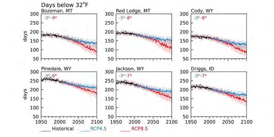
Figure 5-7. Time-series plots of the number of days per year with daily high temperatures above than 90°F (32°C; top) and daily low temperatures below 32°F (0°C; bottom) for selected towns in the Greater Yellowstone Area (GYA). The solid lines are the medians of the 20 models in the MACAv2-METDATA 1950-2005 (black line), and 2006-2099 under Representative Concentration Pathway 4.5 (RCP4.5, blue line) and RCP8.5 (red line). The shaded bands around the lines are the 10th (lower) and 90th (upper) percentiles of the models. The first inset number is the trend (in days/decade) for RCP4.5 (red) and the second number is the trend for RCP8.5 (blue). An asterisk indicates the trend is statistically significant at a 95% confidence level. The small triangles indicate the observed average at National Weather Service sites in the cities for the period of observations (which varies by location). The plotted data are from the MACAv2 METDATA grid cell containing or closest to the location of the city. The observed data are from National Weather Service records (Western Regional Climate Center undated).

Table 5-2. Annual number of days above 90°F (32°C) for the 1986-2005 base period and the change in the number of days for the four future periods under Representative Concentration Pathway 4.5 (RCP4.5) and RCP8.5.

City, State

Table 5-3. Annual number of days below 32°F (0°C) for the 1986-2005 base period and the change in the number of days for the four future periods under Representative Concentration

4.5 (RCP4.5) and RCP8.5.

City, State

Wildfire

The controls of wildfire include energy from the sun, the temperature and humidity of the air, precipitation, wind, and moisture levels of live and dead vegetation and a source of ignition, either from lightning or humans. These factors interact over timescales ranging from minutes to years and longer. Here we discuss some future conditions in the GYA that relate to fire.

The top panel of maps in the Figure Wf-A shows the number of cold days (when the average minimum temperature is below 32°F [0°C]), as a measure of winter warming. Under RCP4.5, the GYA will have nearly 4 weeks fewer cold days by mid century (2041-2060) than the 1986-2005 base period of about 7 months. By the end of century (20802099), there will be 5-6 fewer weeks below freezing than the base period average. Under RCP8.5, the reduction in cold days is even more dramatic (5 weeks for mid century and 10 weeks for end of century).

Fewer cold days in the future suggests that on average winter temperatures will not be cold enough to kill bark beetles and bud worms in GYA forests. Already, warmer temperatures are allowing mountain pine beetles to go through multiple reproductive cycles in a year while extending their range to high-elevation whitebark pine forests (Jewett et al. 2010; Shanahan et al. 2016; Shanahan 2019).

vapor pressure deficit is derived by combining air temperature and relative humidity. It determines the drying capacity of the atmosphere and, as such, affects fuels drying, plant transpiration and plant growth, and more. In conifer forests, high vapor pressure deficits limit tree growth and increase their vulnerability to, and mortality from, drought (Allen et al. 2010; Williams et al. 2013). High vapor pressure deficit also increases the potential for large and severe fires (Seager et al. 2015; Williams et al. 2015; Abatzoglou and Williams 2016). Today, vapor pressure deficits in GYA are greater at lower elevations—where air temperatures are higher and humidity is lower—than at higher elevations (Figure Wf-A, bottom panel). This pattern is projected to be maintained in the future as deficits increase progressively through the century under both RCPs with greater increases at lower elevations.

Figure Wf-A. Top panel: The number of days/year with average minimum temperature below 32°F (0°C) for the 1986-2005 base period (left column) and the changes for future periods under Representative Concentration Pathway 4.5 (RCP4.5) and RCP8.5 in the Greater Yellowstone Area. Bottom panel: Vapor pressure deficit (VPD) for the 1986-2005 base period (left column) and the changes for future periods under Representative Concentration Pathway 4.5 (RCP4.5) and RCP8.5. Vapor pressure deficit is shown as the average for May through September (MJJAS), historically the main months for wildfire. The mapped data are the 20-model means of the MACAv2-METDATA data.

In the future, earlier snowmelt and loss of snowpack as a result of warming winters, followed by warmer summers, longer growing seasons, and more limited soil moisture will increase fire potential at all elevations of the GYA (Westerling et al. 2006). This condition, combined with increased tree mortality, potentially will alter future fire regimes and lead to rapid changes in forest ecosystems (Westerling et al. 2011). Sustained changes in climate and fire disturbance will also affect post-fire recovery of species, thereby changing forest composition and converting forest to grassland at low elevations (Turner et al. 2019). Thus, increased fire activity portends large ecological changes and threatens human health and the communities living in fire-prone areas.

Energy

Projected rising temperatures will alter our demand for energy to heat houses and buildings in winter and cool them in summer. Two widely used temperature-based indicators of energy demand are annual heating degree days and cooling degree days.

Degree days are a measure of how much heating or cooling is needed when the daily average temperature is above or below a “comfortable” outside temperature of 65°F (18°C). For example, if the average daily temperature is 55°F (13°C), there are 10 heating degree days for that date. If the average daily temperature for the next day is 45°F (7.2°C), there are 20 heating degree days for that date and the 2-day total is 30. (If the daily average temperature is 65°F [18°C] or higher, there are zero heating degree days for that date as no energy is needed to heat the home or building.) Cooling degree days are determined similarly when the daily average temperature is above 65°F (18°C) and energy is needed to cool a home or building.

Annual heating or cooling degree days are the total of all daily values throughout the year. Information about future trends in heating and cooling degree days helps the building industry, energy companies, system operators, homeowners, and utilities plan to accommodate the effects of climate change.

Due to its high elevation and northerly location, for the 1986-2005 base period the average number of heating degree days over GYA (10,030) is above the national average (4395), and the annual number of cooling degree days (54) is far below the national average (1216) (NOAA-NCEI undated).

Future warming in winter will decrease the annual heating degree days in GYA (Figure En-A), which will lessen energy demand for commercial and home heating. Relative to the 1986-2005 base period, under RCP4.5 heating degree days decrease by 13% (from 10,030 to 8744) by mid century (2041-2060), and the decrease is 14% (8627) by the end of century (2080-2099). Under RCP8.5, the decreases are 16% (8378) and 31% (6881), respectively, for the two periods.

The percent change in the annual number of heating degree day across GYA cities, which are on average at lower elevations of the GYA, is relatively uniform. (Table En-A, Figure En-B, ), with an average decrease of 14% at mid century (2041-2060) and 19% at the end of century (2080-2099). Under RCP8.5, the average mid-century decrease is 19% and the end of century average decrease is 33%.

Projected summer warming will increase cooling degree days and the need for cooling systems in the GYA, but to a lesser extent than other parts of the country. Mid century (2041-2060) cooling degree days increase by 91% (to 103, presently at 54) and by the end of century they increase by 191% (157, presently 54) in RCP4.5. Under RCP8.5, by mid-century cooling degree days increase by 196% (to 160) and by 844% (510) at the end of century. The need for new or additional cooling largely occurs in lower elevations.

Over the 1986-2005 base period, the annual number of cooling degree days differs substantially across GYA cities (Figure En-C). Under RCP4.5 mid century (2041-2060) annual increases range from 80% (345) at Cody WY to 537% (80) at Pinedale WY (Figure En-C, Table En-B), and by the end of century (2080-2099) cooling degree days increase from 113% (488) at Cody to 867% (130) at Pinedale. (Note that some percentage changes are very large in comparison to heating degree days because they reflect relatively large changes in small numbers, e.g., from 15 at present to 130 by the end of century at Pinedale.) Under RCP8.5 changes in cooling degree days are more extreme and range from 110% (477) at Cody to 805% (135) at Pinedale at mid century, and 267% (1154) at Cody and 3351% (501) at Pinedale at the end of century.

According to the National Academies of Science, space heating consumes more than twice as much energy as cooling nationally (NAS undated). So, the good news is that by mid century, under both RCPs the projected decrease in heating degree days in the towns is roughly five times greater than the increase in cooling degree days, which would mean less annual energy use in the future.

Figure En-A. Annual number of heating degree days (top two rows) and cooling degree days (bottom two rows) in the Greater Yellowstone Area. The 1986-2005 base periods are shown in the left column and changes for the four future periods are shown to the right. The mapped data are the 20-model means computed from MACAv2-METDATA daily average minimum temperature (heating degree days) and daily average maximum temperature (cooling degree days).

Photo credit: Alireza Kaviani/Pexels

Figure En-B. Total annual heating degree days for selected towns in the Greater Yellowstone Area. The solid lines are the medians of the 20 models in the MACAv2-METDATA 1950-2005 (black line), and 2006-2099 under Representative Concentration Pathway 4.5 (RCP4.5, blue line) and RCP8.5 (red line). The shaded bands around the lines are the 10th (lower) and 90th (upper) percentiles of the models The first number in the inset parentheses is the trend (in number/ decade) for RCP4.5 and the second number is the trend for RCP8.5. An asterisk indicates a trend that is statistically significant at a 95% confidence level. The black triangles indicate the observed average at National Weather Service sites in the cities (Western Regional Climate Center undated).

Table En-A. Annual number of heating degree days for the 1986-2005 base period and percent change during the four future periods under Representative Concentration Pathway 4.5 (RCP4.5) and RCP8.5.

City, State

Figure En-C. Total annual cooling degree days for selected towns in the Greater Yellowstone Area. The solid lines are the medians of the 20 models in the MACAv2-METDATA 1950-2005 (black line), and 2006-2099 under Representative Concentration Pathway 4.5 (RCP4.5, blue line) and RCP8.5 (red line). The shaded bands around the lines are the 10th (lower) and 90th (upper) percentiles of the models The first number in the inset parentheses is the trend (in number/ decade) for RCP4.5 and the second number is the trend for RCP8.5. An asterisk indicates a trend that is statistically significant at a 95% confidence level. The black triangles indicate the observed average at National Weather Service sites in the cities (Western Regional Climate Center undated).

Table En-B. Annual number of cooling degree days for the 1986-2005 base period and percent change four future periods under Representative Concentration Pathway 4.5 (RCP4.5) and RCP8.5.

Agriculture

Many aspects of climate affect agriculture, including length of growing season, timing and availability of water, and extreme events such as heat waves, cold snaps, floods, and droughts. Here we examine projected changes in the growing season in the GYA.

The growing season in the GYA today is up to 2 weeks longer than it was in the 1950s, and projections indicate that the growing season in the GYA will be longer and warmer in the future. Under both RCP4.5 and RCP8.5, growing seasons in the future start earlier and end later in the year (Figure Ag-A). The season is lengthened more at low elevations than at high elevations. Under RCP4.5, at mid century (2041-2060) the average growing season length increases by about 3 weeks from the 1986-2005 base-period average of 23 weeks, and by 5 weeks at the end of century (2080-2099). Under RCP8.5, the increases are over 5 weeks and 9 weeks, respectively, for the two periods.

Figure Ag-A. Growing season length in the Greater Yellowstone Area based on temperatures greater than 45°F (7.2°C) (the germination temperature for wheat) for the 1986-2005 base period (left column) and changes over the 21st century under Representative Concentration Pathway 4.5 (RCP4.5, top row) and RCP8.5 (bottom row). The mapped data are 20-model means computed from MACAv2-METDATA daily average temperature.

At representative towns across the GYA, under RCP4.5 (2041-2060) growing season length increases mid century by 3-4 weeks (Figure Ag-B, Table Ag-A), and by 4-6 weeks at the end of century (2080-2099). The growing season lengthens even more under RCP8.5, reaching 4-5 weeks at mid century and 7-11 weeks by the end of century.

Recent climate assessments for the Northern Great Plains (Conant et al. 2018) and Montana (Whitlock et al. 2017) suggest the likelihood of both positive and negative impacts on regional agriculture in the future, but the high elevation and diverse topography of the GYA may be somewhat buffered from the negative impacts that are projected in the Great Plains. For example, the greenhouse effect of elevated CO2 levels may offer the opportunity to grow new plant varieties, and the likelihood of earlier green-up means an earlier grazing season. Still, while some crops and livestock may benefit from longer, warmer growing seasons in the GYA, irrigated and non-irrigated production will need to accommodate earlier snowmelt and timing of runoff, and reduced late-season soil moisture (discussed in Chapter 7). Warmer conditions may also decrease forage quality and support an increase in crop pests (Conant et al. 2018).

Figure Ag-B. Growing season length (base 45°F [7.2°C], the germination temperature of wheat) for selected towns in the Greater Yellowstone Area. The solid lines are the medians of the 20 models in the MACAv2METDATA 1950-2005 (black line), and 2006-2099 under Representative Concentration Pathway 4.5 (RCP4.5, blue line) and RCP8.5 (red line). The shaded bands around the lines are the 10th (lower) and 90th (upper) percentiles of the models. The first inset number is the trend (in days/decade) for RCP4.5 (blue) and the second number is the trend for RCP8.5 (red). An asterisk indicates a trend that is statistically significant at a 95% confidence level. Computed from the MACAv2 METDATA daily mean temperature.

Table Ag-A. Length of growing season based on temperatures greater than 45°F (7.2°C) in weeks for the 1986-2005 base period and changes in the four future periods under Representative Concentration Pathway 4.5 (RCP4.5) and RCP8.5. City, State

Photo courtesy of Rob Van Kirk

SuMMARY OF pROjECTEd TEMpERATuRE ChANGES

о Under both RCP4.5 and RCP8.5, there is 100% model agreement and SNRs >1 in the projected change in mean annual, seasonal, and monthly minimum, maximum, and mean temperatures relative to the 1986-2005 base period in the GYA and the HUC6 watersheds, consistent with previous studies (Whitlock et al. 2017).

о Projected annual warming trends in the HUC6 watersheds are 0.5°F (0.3°C)/decade under RCP4.5 and 1.1-1.2°F (0.6-0.7°C)/decade under RCP8.5. The trends are statistically significant at a 95% confidence level over all HUC6 watersheds.

о Under both RCP4.5 and RCP8.5, warm spells in the GYA increase through the 21st century (Figure 5-3). Under RCP8.5, by the end of the century the warm spell duration index is greater than 200 days out of the year. The steady increase in the warm spell duration index represents a fundamental warming of the daily maximum temperature, as opposed to heatwaves, which are extremes relative to the prevailing climatology.

о The modeled mean annual number of cold days (below 32°F [0°C]) and hot days (above 90°F [32°C]) at selected towns in the GYA agree with the 1950-2005 mean of observations, and the projected trends in the number of cold and hot days are statistically significant under both RCP4.5 and RCP8.5, also consistent with previous studies (Whitlock et al. 2017; Conant et al. 2018).

о In the HUC6 watersheds, under RCP4.5 mid century (2041-2060) decreases in the number of cold days/yr range from 23 at Red Lodge MT (base period mean 186), to 28 at Bozeman MT (base period mean 175), and 29 at Jackson WY (base period mean 229). By the end of century (2080-2099) decreases range from 36 at Red Lodge and Pinedale WY to 41 days at Bozeman and Jackson. Under RCP8.5 decreases range from 32 days at Red Lodge to 38 days at Jackson and Bozeman by mid century, and from 63 days at Pinedale to 77 days at Bozeman by the end of century.

о In the HUC6 watersheds, under RCP4.5 mid century (2041-2060) increases in hot days/ yr range from 5 at Pinedale WY (base period mean 0) and Jackson WY (base period mean 0), to 23 at Bozeman MT (base period mean 9) and Cody WY (base period mean 11). By the end of century (2080-2099) increases in hot days/yr range from 9 at Pinedale and 10 at Jackson, to 31 in Bozeman and 32 in Cody. Under RCP8.5 increases in hot days/yr range from 10 in Pinedale and Jackson to 32 at Cody by mid century, and from 42 at Pinedale and Jackson to 64 at Cody at the end of century.

о Under RCP4.5, at mid century (2041-2060) the average growing season length increases by about 3 weeks from the 1986-2005 base-period average of 23 weeks, and by 5 weeks at the end of century (2080-2099). Under RCP8.5, the increases are over 5 weeks and 9 weeks, respectively, for the two periods.

о Projected warmer cold season temperatures will reduce energy demands for heating and warmer summers will increase energy demands for cooling. The energy reduction for heating could be as much as five times greater than the increase for cooling.

о In the future, earlier snowmelt, and loss of snowpack during warmer winters followed by warmer summers and longer growing seasons will increase fire potential at all elevations of GYA. Increased fire activity portends large ecological changes and threatens human health and the communities living in fire-prone areas.

ChApTER 5 AppENdIx—A dEEpER LOOk

Climate variables

Table A5-1. The climate variables discussed in this chapter.

Variable Description Source

Air temperature

Vapor pressure deficit

Annual number of days below 32°F (0°C)

Annual number of days above 90°F (32°C)

Growing season lengtha

Heating degree days

Cooling degree days

Maximum, minimum, and average at a height of 2 meters (6.6 ft)

A measure of the fuel-drying power of the atmosphere based on temperature and relative humidity, used to evaluate wildfire potential

MACAv2-METDATA

Warm spell

Cold spell

Kilo Pascals (kPa)

Count of the days/yr. Important for growth of plants. Derived from MACAv2-METDATA Days

Count of the days/yr. Important for human and ecological health

An index of the number of days between the first 6-day period and last 6-day period with average air temperature greater than 42°F (5°C). Important for agriculture and forests.

The total degrees/yr that the daily average temperature is less than 65°F (5°C). Important for energy demands for heating.

The total degrees/yr that the daily average temperature is greater than 65°F (5°C). Important for energy demands for cooling.

A sequence of 6 or more days in which the daily maximum temperature exceeds the 90th percentile of daily maximum temperature for a 5-day running window surrounding this day during the baseline period (1961-1990)

A sequence of 6 or more days in which the daily maximum temperature is below the 10th percentile of daily minimum temperature for a 5-day running window surrounding this day during the baseline period (1961-1990)

Derived from MACAv2-METDATA Days

Derived from MACAv2-METDATA based on Climdex Days

Derived from MACAv2-METDATA Degree days

Derived from MACAv2-METDATA Degree days

Derived from MACAv2-METDATA Days

Derived from MACAv2-METDATA Days

a Growing season length depends on the geographic location and the particular type of plant or plants. Because frost is possible throughout the GYA on any day of the year, we chose to use the Climdex index (which generally applies to the 45°F (7.2°C) germination temperature of wheat.). Climdex is a collaborative international project that develops and maintains a wide array of climate extreme variables for climate research (see https://www.climdex.org/about/project/ and https://www.climateextremes.org. au/).

Figures supporting Chapter 5

Figure A5-1. Seasonal mean temperature (average of minimum and maximum temperatures) in the Greater Yellowstone Area for the 1986-2005 base period (left column), Representative Concentration Pathway 8.5 (RCP8.5, four center columns), and the end of the 21st century under RCP4.5 (right column). The seasons (e.g., December-February [DJF]) are arranged in rows and the future periods (e.g., 2021-2040) are in columns. The mapped data are the 20-model means of the MACAv2-METDATA.

Figure A5-2. Change in seasonal mean temperature (average of minimum and maximum temperatures) in the Greater Yellowstone Area under Representative Concentration Pathway 8.5 (RCP8.5, left four columns) and at the end of the 21st century under RCP4.5 (right column). The seasons (e.g., December-February [DJF]) are arranged in rows and the changes relative to the 1986-2005 base period for each future period (e.g., 2021-2040) are in columns. The mapped data are the 20-model means of the MACAv2-METDATA.

Figure A5.3. The range of projected change in seasonal mean of maximum air temperature under Representative Concentration Pathway 8.5 (RCP8.5) for the Hydrologic Unit Code 6 (HUC6) watersheds, as simulated individually by the 20 downscaled global climate models (GCMs) in the MACAv2-METDATA. The seasons are in columns and the future period are in rows. Within each block the GCM names and their mean (Mean Model) are labeled on the left and the HUC6 watersheds are labeled at the bottom. See Table A4-1 for model details.

LITERATuRE CITEd

Abatzoglou JT, Williams AP. 2016. Impact of anthropogenic climate change on wildfire across western US forests. Proceedings of the National Academy of Sciences 113:11770-5.

Allen CD, Macalady AK, Chenchouni H, Bachelet D, McDowell N, vennetier M, Kitzberger T, Rigling A, Breshears DD, Hogg EH, Gonzalez P, Fensham R, Zhang Z, Castro J, Demidova N, Lim J-H, Allard G, Running SW, Semerci A, Cobb N. 2010. A global overview of drought and heat-induced tree mortality reveals emerging climate change risks for forests. Forest Ecology and Management 259(4):660-84. https://doi.org/10.1016/j.foreco.2009.09.001.

Conant RT, Kluck D, Anderson M, Badger A, Boustead BM, Derner J, Farris L, Hayes M, Livneh B, McNeeley S, Peck D, Shulski M, Small v. 2018. Northern Great Plains [chapter 22]. In: Impacts, Risks, and Adaptation in the United States: Fourth National Climate Assessment, vol II. In: Reidmiller DR, Avery CW, Easterling DR, Kunkel KE, Lewis KLM, Maycock TK, Stewart BC, editors. Washington DC: US Global Change Research Program. p 941-86. https://doi.org/10.7930/NCA4.2018.CH22.

[IPCC] Intergovernmental Panel on Climate Change. 2014. Climate Change 2014: synthesis report: contribution of working groups I, II and III to the Fifth Assessment Report of the Intergovernmental Panel on Climate Change. Pachauri RK, Meyer LA, eds. Geneva Switzerland: Intergovernmental Panel on Climate Change. 151 p.

Jewett JT, Lawrence RL, Marshall LA, Gessler PE, Powell SL, Savage SL. 2011. Spatiotemporal relationships between climate and whitebark pine mortality in the Greater Yellowstone Ecosystem. Forest Science 57(4): 320-35. https://doi.org/10.1093/forestscience/57.4.320.

[NAS] National Academy of Sciences, Engineering, Medicine. [undated][. What you need to know about energy: energy efficiency [webpage]. Available online http://needtoknow.nas.edu/energy/energyefficiency/heating-cooling/. Accessed Feb 2021.

[NOAA-NCEI] National Oceanic and Atmospheric Administration-National Centers for Environmental Information. [undated]. Comparative climatic data [webpage]. Available online https://www.ncdc.noaa. gov/ghcn/comparative-climatic-data. Accessed 13 May 2021.

Seager R, Hooks A, Williams AP, Cook B, Nakamura J, Henderson N. 2015 (Jun). Climatology, variability, and trends in the US vapor pressure deficit, an important fire-related meteorological quantity. Journal of Applied Meteorology and Climatology 54:1121-41. https://doi.org/10.1175/JAMC-D-14-0321.1.

Shanahan E. 2019. An uncertain future: the persistence of whitebark pine in the Greater Yellowstone Ecosystem. Yellowstone Science 27(1):67-71.

Shanahan E, Irvine KM, Thoma D, Wilmoth S, Ray A, Legg K, Shovic H. 2016 (Dec). Whitebark pine mortality related to white pine blister rust, mountain pine beetle outbreak, and water availability. Ecosphere 7(12):e01610. https://doi.org/10.1002/ecs2.1610.

Turner MG, Braziunas KH, Hansen WD, Harvey BJ. 2019. Short-interval severe fire erodes the resilience of subalpine lodgepole pine forests. Proceedings of the National Academy of Sciences 116:11319-28.

Westerling AL, Hidalgo HG, Cayan DR, Swetnam TW. 2006. Warming and earlier spring increase western US forest wildfire activity. Science 313:940-3.

Westerling AL, Turner MG, Smithwick EAH, Romme WH, Ryan MG. 2011. Continued warming could transform Greater Yellowstone fire regimes by mid-21st century. Proceedings of the National Academy of Sciences USA 108:13165-70. https://doi.org/10.1073/pnas.1110199108.

Western Regional Climate Center. [undated]. Local climate data summaries [webpage]. Available online https://wrcc.dri.edu/summary/lcd.html. Accessed Jan 2020.

Whitlock C, Cross W, Maxwell B, Silverman N, Wade AA. 2017. 2017 Montana Climate Assessment. Bozeman and Missoula MT: Montana State University and University of Montana, Montana Institute on Ecosystems. 318 p. doi:10.15788/m2ww8w.

Williams AP, Seager R, Macalady AK, Berkelhammer M, Crimmins MA, Swetnam TW, Trugman AT, Buenning N, Noone D, McDowell NG, Hryniw N, Mora CI, Rahn T. 2015. Correlations between components of the water balance and burned area reveal new insights for predicting forest fire area in the southwest United States. International Journal of Wildland Fire 24(1):14-26. https://doi.org/10.1071/WF14023.

Williams P, Allen CD, Macalady AK, Griffin D, Woodhouse CA, Meko DM, Swetnam TW, Rauscher SA, Seager R, Grissino-Mayer HD, Dean JS, Cook ER, Gangodagamage C, Cai M, McDowell NG. 2013. Temperature as a potent driver of regional forest drought stress and tree mortality. Nature Climate Change 3:292-7.

Virga over Montana’s Gallatin Valley

Photo courtesy of Suzi Taylor

6. FUTURE PRECIPITATION PROJECTIONS FOR THE GREATER YELLOWSTONE AREA

Steven Hostetler and Jay Alder

kEY MESSAGES

о Under RCP4.5, mean annual precipitation in the GYA is projected to increase 7% by mid century (2041-2060) and 8% by the end of century (2081-2099) relative to the 1986-2005 base period. Under RCP8.5, the projected increases are 9 and 15% for these periods, respectively. [medium confidence, >80% model agreement and SNR >1]

о The projected increase in mean annual precipitation is attributed to increases during the December through April cold season, particularly in March and April when the snow-rain transition occurs. [high confidence, >80% model agreement and SNR >1]

о By the end of the century (2081-2099), the wettest month shifts from May to April in the Big Horn, Upper Green, and Snake Headwaters watersheds. These shifts occur by mid century (2061-2080) and are amplified under RCP8.5. [medium confidence, 60-80% model agreement]

о In the HUC6 watersheds, statistically significant positive trends in mean annual precipitation range from 0.17-0.23 inches/decade (0.43-0.58 cm/decade) under RCP4.5, and 0.35-0.52 inches/decade (0.89-1.3 cm/decade) under RCP8.5. Given the spread in the models, RCP4.5 and RCP8.5 trends are not significantly different over the 21st century. [medium confidence, significance in trends]

INTROduCTION

In this chapter, we analyze projected changes in mean annual, seasonal, and monthly precipitation in the GYA and the HUC6 watersheds. We summarize the main points of the projections and provide the details of the projections through time and space with interrelated maps, graphs, and checkerboard plots.

ANNuAL ANd SEASONAL pRECIpITATION

OvER ThE GYA

The distribution of precipitation over GYA is influenced by the direction from which the moisture arrives, which varies seasonally and topographically (see Chapter 2). As evident in Figure 6-1, that influence is particularly strong during the winter and spring when most precipitation falls as snow at higher elevations. Under RCP4.5, projected mean annual precipitation over GYA increases by 1.4 inches (3.6 cm; 5.4%) over the 2021-2040 period to 2.4 inches (6.1 cm; 9.0%) in 2080-2099. Under RCP8.5, the increases for these periods are 1.6 inches (4.1 cm; 6.0%) and 3.9 inches (9.9 cm; 14.6%). Throughout the 21st century, the largest increase for both RCPs is in spring (MAM) followed by winter (DJF). During summer, the changes range from small increases (0.1 inches [0.3 cm]; 2.2%) to small decreases (-0.2 inches [-0.5 cm]; 2.8%). Fall precipitation increases somewhat until 2060 and decreases thereafter. A 1 inch (2.5-cm) change in precipitation over the entire GYA amounts to roughly 1,000,000 acre-ft (123,348,000 m3) of water.1

Figure 6-1. Seasonal mean precipitation in the Greater Yellowstone Area for the 1986-2005 base period (left column), changes under Representative Concentration Pathway 4.5 (RCP4.5, four center columns), and the end of the 21st century under RCP8.5 (right column). The seasons (e.g., December-February [DJF]) are arranged in rows and the differences relative to the 1986-2005 base period for each future period (e.g., 2021-2040) are in columns. The data shown are the 20-model means of the MACAv2-METDATA. See Figure A6-1 in the appendix to this chapter for all RCP8.5 maps.

1 For comparison, the volume of Yellowstone Lake is just over 12,000,000 acre-ft (14,801,760,000 m3) (NPS undated).

There is little change in the projected maximum length of wet spells under either RCP4.5 or RCP8.5 across the GYA (Figure 6-2). There is also little projected change in the maximum length of dry spells. As indicated by the increased upper portion of the shaded bands, after 2050 some models simulate an increase in the number of days for the maximum dry spell length under RCP8.5.

Figure 6-2. Length of wet spells A) and B) and dry spells C) and D) in the Greater Yellowstone Area under Representative Concentration Pathway 4.5 (RCP4.5) and RCP8.5. The heavy lines are the 20-model median and the shaded bands indicate the 10th (bottom) to 90th (top) percentiles around the medians. The black portion is the 1950-2005 period and the colored portion is for the RCP simulations (2006-2099). Indexes are calculated from the MACAv2-METDATA precipitation data. See Table A6-1 in the Appendix for details of how wet and dry spells are calculated.

pRECIpITATION OvER ThE huC6 WATERShEdS

For the 1986-2005 base period, mean annual precipitation in the GYA ranges from 22 inches (56 cm) in the Upper Green watershed to 31 inches (79 cm) in the Snake Headwaters watershed (Figure 6-3 and Table 6-1). The positive trend between 1950 and 2005 (here and in Chapter 3) continues under both RCPs. The trends are statistically significant at the 95% confidence level in all HUC6 watersheds under both RCPs. Although the amount of annual precipitation varies among the HUC6 watersheds, as indicated by the inset numbers, the trends (in inches/decade) are similar. Under RCP8.5, the projected trends are roughly twice those of RCP4.5. The precipitation trends are more gradual than those of temperature described in Chapter 5 and the annual values of the RCPs are not statistically different, as indicated by overlap of the medians and the range and overlap of the shaded bands.

Figure 6-3. Time-series plots of the 1950-2099 mean annual precipitation for the Hydrologic Unit Code 6 (HUC6) watersheds. The solid lines are the medians of the 20 models in the MACAv2METDATA data, from 1950-2005 (black line), and 2006-2099 for Representative Concentration Pathway 4.5 (RCP4.5, blue line) and RCP8.5 (red line). The shaded bands around the lines are the 10th (lower) and 90th (upper) percentiles of the models. The first number in the inset in each panel is the trend (in inches/decade) for RCP4.5 and the second number is the trend for RCP8.5. An asterisk indicates that the trend is statistically significant at a 95% confidence level.

Relative to the 1986-2005 base period, under RCP4.5 projected mean annual precipitation in the GYA is 7% greater by mid century (2041-2060) and 8% greater at the end of century (2081-2099) (Table 6-1). Under RCP8.5, the projected increases are 9 and 15% for these periods, respectively. The increases are essentially uniformly distributed over the HUC6 watersheds. Again, the absolute changes are relatively small but represent a substantial amount of water when totaled over the area of a HUC or the GYA.

Table 6-1. Mean annual precipitation in the Greater Yellowstone Area (GYA) and Hydrologic Unit Code 6 (HUC6) watersheds for the 1986-2005 base period and change during the four future periods under Representative Concentration Pathway 4.5 (RCP4.5) and RCP8.5. The units are in inches and the parenthetical values are percent change. Watershed

ThE SEASONAL CYCLE OF pRECIpITATION

Projected mean monthly precipitation across the HUC6 watersheds, like mean annual precipitation across the GYA, shows the influence of topography and varies by season (Figure 6-4). For the 1986-2005 base period, May is the wettest month in the GYA. Over the northern and eastern watersheds (Missouri Headwaters, Upper Yellowstone, and Big Horn), precipitation increases throughout the winter and peaks in May before declining to summer minima (Figure 6-4). The southern and western watersheds (Upper Green, Snake Headwaters, and Upper Snake) receive more-or-less uniform precipitation throughout winter and spring before it declines to summer minima after May. As shown in Figure 6-4, under RCP4.5 an increase in January through April precipitation becomes greater through the century and, by the end of the century (20812099) the wettest month shifts from May to April in the Big Horn, Upper Green, and Snake Headwaters watersheds. These shifts occur by mid century (2061-2080) and are amplified under RCP8.5. This projected change in the seasonality of precipitation contributes to altering the timing of future runoff.

[U]nder RCP4.5 an increase in January through April precipitation becomes greater through the century and, by the end of the century (2081-2099) the wettest month shifts from May to April in the Big Horn, Upper Green, and Snake Headwaters watersheds. These shifts occur by mid century (2061-2080) and are amplified under RCP8.5. This projected change in the seasonality of precipitation contributes to altering the timing of future runoff.

Younts Peak, headwaters of the Yellowstone River, Bridger-Teton National Forest, Wyoming

Photo courtesy of Scott Bischke

Figure 6-4. The seasonal cycle of mean monthly precipitation for the Hydrologic Unit Code 6 (HUC6) watersheds under Representative Concentration Pathway 4.5 (RCP4.5) and RCP8.5. The black line shows 1986-2005 base period. The colored lines are the 20-model means of the MACAv2-METDATA data for the periods indicated in the legend at the bottom. The shaded bands are the model spread around the respective colored mean lines.

Checkerboard plots for the HUC6 watersheds and the GYA (Figure 6-5) further illustrate the nature of the projected 21st-century precipitation changes. As in Figure 5-6, each rectangular grid in Figure 6-5 illustrates the differences (anomalies) between a given period and the base period (e.g., 2021-2040 minus 1986-2005) broken down by monthly and annual means, for the GYA and each HUC6 watershed.

Figure 6-5. Change in projected mean monthly and annual precipitation in the Greater Yellowstone Area (GYA) and Hydrologic Unit Code 6 (HUC6) watersheds. The columns from left to right show changes for each future period (e.g., 2021-2040) relative to the 1986-2005 base period with Representative Concentration Pathway 4.5 (RCP4.5) on the top row and RCP8.5 on the bottom row. In each RCP figure, the months and annual mean (AVG) run from left to right across the horizontal axis on the bottom and the HUC6 watersheds and GYA run along the vertical axis on the left. Colored cells indicate >80% (more than 16 of the 20 models) agree on the sign of the change in the median value (positive or negative). A slash in a colored cell indicates that 60-80% of the models (12-16 out of 20) agree on the sign of the change, and an X in a box indicates that fewer than 60% (<12) of the models agree on the sign of the change. A black dot in a box indicates that the ensemble mean value of the future change is greater than the inter-model standard deviation (SNR >1), an indicator of significance of the change (see Chapter 1 for details). The data shown are the 20-model means of the MACAv2-METDATA data.

Changes in mean monthly precipitation are more variable both among HUC6 watersheds and between RCPs than is the case with temperature (Figures 5-5, 5-6, 5-7). The four time periods all show increases in cold season (November through April) precipitation. The number of boxes displaying model agreement and SNRs >1 increases through time as the magnitude of future changes become greater. Subtle differences across the HUC6 watersheds for a given month reflect spatial differences in precipitation shown in Figure 6-1.

Changes in mean monthly precipitation are more variable both among HUC6 watersheds and between RCPs than is the case with temperature. … [However,] increases in cold season (November through April) precipitation are clear.

From June through October, precipitation changes are mixed in sign and vary by HUC6 watershed. Slightly more drying is evident in the northern and eastern watersheds. There is less agreement of the projected change among the models than there is during the cold season and no boxes display SNR >1. Lack of significance and model agreement is attributed to the wide range of summer precipitation simulated by the 20 GCMs (Figure A6-2). While projected increases in winter and spring are consistent among models, projections for the warm season (June through October) are a mix of increases, decreases, and no change that vary by climate model and watershed. Decreased precipitation in summer and increased precipitation in fall in some HUC6 watersheds are consistent with observed trends since 1950 (see Chapter 3). Seasonal contrasts in model agreement and model spread suggest that the underlying mechanisms of winter precipitation (e.g., changes in storm tracks and greater capacity for a warming atmosphere to hold moisture) are shared among the models, whereas the primary form of summer precipitation (convection) is more challenging to model and less consistent among models. It also reveals limitations in the ability to statistically downscale convective precipitation.

SuMMARY OF pROjECTEd pRECIpITATION ChANGES

о Under both RCP4.5 and RCP8.5, there is a high level of model agreement in the projected increase in mean annual precipitation over the GYA and the HUC6 watersheds. The increase is attributed to increases in winter and spring. [85 to 100% model agreement and SNRs >1]

о Under both RCP4.5 and RCP8.5, the models project a mix of increases and decreases in summer precipitation with generally less than 60% model agreement. There are no SNRs >1 in the projected changes in summer precipitation.

о There is little change in the projected length of wet spells under either RCP4.5 or RCP8.5 across the GYA (Figure 6-2). There is also little projected change in the maximum length of dry spells; however, after 2050 some models simulate an increase in the length of dry spells under RCP8.5.

о Statistically significant positive trends in mean annual precipitation are projected for all HUC6 watersheds under both RCP4.5 and RCP8.5, but the trends for the RCPs are not statistically different.

ChApTER 6 AppENdIx—A dEEpER LOOk

Table and figures supporting Chapter 6

Table A6-1. The climate variables discussed in this chapter.

Variable Description

Wet spell

Dry spell

Maximum number of consecutive days/yr with daily precipitation amounts of at least a trace (>1 mm).

Maximum number of consecutive days/yr with daily precipitation amounts of less than a trace (<1 mm).

Source

Units

Derived from MACAv2-METDATA Days

Derived from MACAv2-METDATA Days

Figure A6-1. Seasonal mean precipitation in the Greater Yellowstone Area for the 1986-2005 base period (left column), changes under Representative Concentration Pathway 8.5 (RCP8.5, four center columns), and the end of the 21st century under RCP4.5 (right column). The seasons (e.g., DecemberFebruary [DJF]) are arranged in rows from top to bottom and the changes relative to the 1986-2005 base period for each future period (e.g., 2021-2040) are in columns. The data shown are the 20-model means of the MACAv2-METDATA data.

Figure A6-2. The range of projected change in seasonal mean precipitation under Representative Concentration Pathway 8.5 (RCP8.5) for the Hydrologic Unit Code 6 (HUC6) watersheds, as simulated individually by the 20 downscaled global climate models (GCMs) in the MACAv2-METDATA. The seasons are in columns and the future period are in rows. Within each block of the GCM names and their mean (Mean Model) are labeled on the left and the HUC6 basins are labeled at the bottom. See Table A4-1 for model details.

LITERATuRE CITEd

[NPS] National Park Service. [undated]. Water [webpage]. Available online https://www.nps.gov/ yell/learn/nature/water.htm#:~:text=Yellowstone%20Lake%20is%20the%20largest, December%20 to%20May%20or%20June. Accessed 30 Apr 2021.

High-country limnological research at Spider Lake in the upper Wind River watershed, Wind River Indian Reservation, Wyoming

Photo courtesy of Bryan Shuman

7. FUTURE WATER PROJECTIONS FOR THE GREATER YELLOWSTONE AREA

Steven Hostetler and Jay Alder

kEY MESSAGES

о Snow governs the annual water cycle of GYA. Under RCP4.5, the total area of the GYA dominated by winter snowfall decreases from 59% during the base period (1986-2005) to 27% at mid century (2041-2060) and to 11% by the end of century (2081-2099). Under RCP8.5, the extent of snow-dominant area decreases to 17% and to 1% for the same time periods, respectively. [high confidence, 100% model agreement and SNR >1]

о Total annual runoff in GYA is projected to increase by about 1% by mid century (20412060) and by 2% at the end of century (2081-2099) under RCP4.5, and increase by 2% and 3% for same time periods, respectively, under RCP8.5. [low to medium confidence, <60% to 80% model agreement, SNR <1]

о The seasonality of runoff is projected to change as snowfall declines and snowpack melts earlier under both RCP4.5 and RCP8.5. [high confidence, >80% model agreement and SNR >1]

о The biggest changes are at mid and high elevations where runoff from snowmelt increases in spring (March through May) and decreases in summer (June through August). Timing of peak runoff is projected to shift by 1-2 months earlier in the year in the later part of the century under RCP8.5. [high confidence, >80% model agreement and SNR >1]

о On an annual basis, precipitation (P) over the GYA exceeds potential evapotranspiration (PET), but the reverse is true in summer, particularly at lower elevations, leading to a seasonal water deficit that is projected to increase in the future. [high confidence, >80% model agreement and SNR >1]

о Summer PET is projected to increase in the future so the summer water deficit is projected to increase by 25% by mid century (2041-2060) and by 36% at the end of century (2081-2099) under RCP4.5. Under RCP8.5, projected deficit increases are 35% by mid century and 79% by the end of century. [high confidence, >80% model agreement and SNR >1]

о For the 1986-2005 base period over the GYA, modeled summer soil moisture levels are about 25% of capacity at low elevations and 50% of capacity at higher elevations. Under RCP4.5 June-October soil moisture saturation decreases by 23% mid century and 33% by the end of the century. Under RCP8.5 June-October soil moisture saturation decreases by 30% at mid century and 56% by the end of the century [high confidence, > 80% model agreement and SNR >1]

The Water Balance Model

Water balance is the difference between water gains and losses over an area like the GYA or a HUC6 watershed. Gains come from precipitation in the form of rain, sleet, or snow. Losses occur through runoff (draining away of water on the surface), evapotranspiration (evaporation from bare soils plus transpiration from vegetation), sublimation of snow (evaporation directly from the snow without melting), and change in water stored as snowpack or in the ground. The water balance model applied here (see figure) accounts for these various components of the water balance monthly.

о Potential evapotranspiration (PET) is the amount of evapotranspiration that would occur if unlimited water were available, such as from an open pan of water or well irrigated crops.

Schematic diagram of the water balance model. Monthly precipitation and temperature inputs are from the MACAv2METDATA data set and solar radiation is determined as a function of latitude and day of year (Hostetler and Alder 2016).

о Actual evapotranspiration is the amount of evapotranspiration that occurs under actual moisture conditions. Soil moisture is the primary limiter of water available for evapotranspiration. When soil moisture levels decline, evapotranspiration is increasingly limited as it becomes more difficult to extract water from the soil.

о The seasonal water deficit or precipitation minus evapotranspiration (P-PET) is the difference between supply (precipitation, P) and atmospheric demand (potential evapotranspiration, PET). It is a measure of climatological wetness (P greater than PET) or dryness (P less than PET) in an area such as the GYA (McCabe and Wolock 2015; NOAA-NCEI undated).

о Runoff is the excess water available from precipitation and snowmelt that does not get evaporated, sublimated, or absorbed in the soil. It is a depth of water in a given area (e.g., the GYA or HUC6 watersheds) that would be available for routing into streamflow and groundwater. (More detailed hydrologic models are needed to simulate routing of runoff into stream and groundwater networks.)

Additional details on the water balance model are provided in the appendix to this chapter.

INTROduCTION

In this chapter we present aspects of projected changes in water in GYA. We apply a water balance model to evaluate climate-driven changes in the water cycle (for more detail see box and the appendix to this chapter). The relatively simple model uses monthly average air temperature and precipitation from the MACAv2-METDATA data and the seasonal cycle of potential solar radiation as inputs. The water balance model output is produced over the same 4-km (2.5-mile) grid cells as the temperature and precipitation data.

SNOW

The annual water cycle of the GYA is governed by snow accumulation during winter and snowmelt during spring and summer. Summer thunderstorms frequently increase streamflows and augment soil moisture for periods of days, but snowpack determines the annual availability of water for ecosystems, agriculture, and communities in the GYA.

The annual water cycle of the GYA is governed by snow accumulation during winter and snowmelt during spring and summer… snowpack determines the annual availability of water for ecosystems, agriculture, and communities in the GYA.

As indicated by tree-ring analyses and observations (see Chapters 2 and 3), the snow regime in the GYA (and elsewhere in the West) is already changing. Precipitation in the GYA is projected to increase somewhat through the 21st century, but issues of concern for snow in the future are:

о How much precipitation will fall as snow versus rain?

о How much water will accumulate in, or be lost from, the snowpack?

о What will be the rate and timing of snowmelt?

As simulated by the water balance model, ongoing changes in snow in the GYA are projected to continue into the future (Figure 7-1 and Table 7-1, also Figure A7-1 in the appendix to this chapter). The range of colors in the time-elevation plots in Figures 7-1 and A7-1 illustrate that, just as today, future periods display trends, as well as year-to-year variability, in snow. While the overall trends among the HUC6 watersheds are similar, details—for example, the large range and evolution of the rain-to-snow transition zone—reflect both intra- and inter-HUC6 differences in topography, location, and variation of winter temperatures around freezing.

Figure 7-1. The 1986-2099 annual snow regime for the Greater Yellowstone Area and Hydrologic Unit Code 6 (HUC6) watersheds under Representative Concentration Pathway 4.5 (RCP4.5), as simulated by the water balance model. The five maps across the top display the ratio of maximum snow water equivalent (SWE) to total cold-season (Oct-Apr) precipitation (P) SWE:P for the indicated time periods (see appendix to this chapter for details on the ratio). The pie charts inset in the maps show the fraction of GYA area within each SWE:P category. The time-elevation plots for the HUC6 watersheds in the bottom two rows display the trend in SWE:P ratio from 1986-2099 averaged over 330 ft (100 m) elevation bands. Gray shading indicates elevations not present in the HUCs. See Figure A7-1 for RCP8.5.

Table 7-1. Percent area of the Greater Yellowstone Area (GYA) by precipitation type for the 1986-2005 base period, and the four future periods under Representative Concentration Pathway 4.5 (RCP4.5, blue numbers) and RCP8.5 (red numbers), as simulated by the water balance model. See the appendix at the end of this chapter for details on how the precipitation zones are delineated.

The map for the 1986-2005 base period shows that the rain-dominated zone amounts to 10% of the total area of the GYA (Table 7-1) and is characteristic of elevations below about 5000 ft (1500 m). The rain-snow mix zone amounts to 32% of the GYA and generally occurs at elevations between 5000-7000 ft (1500-2100 m), and the snow-dominant area amounts to 59% of the area above 7000 ft (2100 m). There is a progressive upward elevational shift in these zones in response to the warming under both RCPs. Under RCP4.5, by mid century (2041-2060) the area dominated by rain more than doubles to 23%, the area of rain-snow mix increases from 32% to 50%, and the snow dominant area shrinks from 59% to 27% of the total area. By the end of century, the area of rain-snow mix increases to 62% and the snow-dominant area is further reduced to 11%. These changes stabilize around 2070 and, at the end of century, only areas above about 9000 ft (2700 m) remain snow dominant. The trends are more dramatic under RCP8.5 (Table 7-1, also Figure A7-1 in the appendix to this chapter). By 2041-2060, the loss of the snow-dominant areas under RCP8.5 are similar to those of RCP4.5 for the 2061-2080 period, and by the end of century snowdominant areas are lost except at the highest elevations of the Upper Yellowstone and Upper Green watersheds.

The 21st-century changes in the distribution of the snow regime in the HUC6 watersheds shown in Figures 7-1 and A7-1 are summarized by trends in the amount of liquid water stored in the snowpack (snow water equivalent, or SWE) on April 1st (Figure 7-2). All watersheds exhibit statistically significant negative trends in the SWE over the 1986-2005 base period that continue through the 21st century under both RCPs. Under RCP4.5, mid century (2041-2060) decreases range from about 24% (from 3.1 inches [7.9 cm] to 2.4 inches [6.1 cm]) in the Upper Yellowstone and Big Horn watersheds to about 30% in the western Upper Snake and Missouri Headwaters watersheds; by the end of century (2081-2099) the decreases range from 38% in the Upper Yellowstone and Big Horn watersheds to 44% in the Upper Snake and Missouri Headwaters watersheds. Under RCP8.5, mid century decreases range from 31% in the Big Horn and Upper Green watersheds to 39% in the Upper Snake and Missouri Headwaters watersheds, and by the end of century decreases range from 65% in the Upper Yellowstone to 73% in the Upper Snake and Missouri Headwaters watersheds.

Figure 7-2. Time-series plots of the 1950-2099 April 1 amount of water stored in the snowpack (snow water equivalent, or SWE), as simulated by the water balance model. The solid lines are the medians of the 20 simulations that used the MACAv2-METDATA data, from 1950-2005 (black line), and 2006-2099 for Representative Concentration Pathway 4.5 (RCP4.5, blue line) and RCP8.5 (red line). The shaded bands around the lines are the 10th (lower) and 90th (upper) percentiles of the models. The first number in the inset in each panel is the trend (in inches/decade) for RCP4.5 and the second number is the trend for RCP8.5. An asterisk indicates that the trend is statistically significant at a 95% confidence level.

Checkerboard plots further illustrate changes in SWE in the HUC6 watersheds (Figure 7-3). As in the previous checkerboard figures, each rectangular grid illustrates the differences (anomalies) between a given period and the base period (e.g., 2021-2040 minus 1986-2005) broken down by monthly and annual means, for the GYA and each HUC6 watershed.

Figure 7-3. Change in the monthly and annual amount of water stored in the snowpack (snow water equivalent) over the Hydrologic Unit Code 6 (HUC6) watersheds and Greater Yellowstone Area (GYA), as simulated by the water balance model. The columns from left to right show changes for each future period (e.g., 2021-2040) relative to the 1986-2005 base period with Representative Concentration Pathway 4.5 (RCP4.5) on the top row and RCP8.5 on the bottom row. In each RCP figure, the months and annual mean (AVG) run from left to right across the horizontal axis on the bottom and the HUC6 watersheds and GYA run along the vertical axis on the left. Colored cells indicate >80% (more than 16 of the 20 models) agree on the sign of the change in the median value (positive or negative). A slash in a colored cell indicates that 60-80% of the models (12-16 out of 20) agree on the sign of the change, and an X in a box indicates that fewer than 60% (<12) of the models agree on the sign of the change. A black dot in a box indicates that the ensemble mean value of the future change is greater than the inter-model standard deviation (SNR >1), an indicator of significance of the change (see Chapter 1 for details). Shown are the 20 model means of the simulations that used the MACAv2-METDATA data as model input.

Beginning in the 2021-2040 period, there is a high level of model agreement with SNRs >1 in the loss of snowpack (SWE) in all the HUC6 watersheds. The greatest absolute losses are in the Snake Headwaters, which receives most of its precipitation from Pacific storms during the cold season. By 2041-2060, the monthly loss of snowpack is unidirectional and evident in all HUC6 watersheds, in all future periods, and under both RCPs. There is greater than 95% model agreement (19 to 20 out of 20 models) and SNRs >1 for the GYA and HUC6 watersheds from November through May when snowpack is present.

RuNOFF

Runoff considered by elevation

As simulated by the water balance model, over the 1986-2005 base period the source of runoff in the GYA primarily originates from snowmelt at elevations between 6000 and 10,000 ft (1800 and 3000 m), where snowpack accumulates (left column, Figure 7-4). Sixty three percent of annual precipitation over the GYA becomes runoff and in some areas of the GYA up to 80% of annual runoff is supplied by snowmelt. Runoff begins at lower- and mid-elevations in March and April and generally peaks in May or June in the HUC6 watersheds (left column, Figure 7-5).

Figure 7-4. Seasonal mean runoff in the Greater Yellowstone Area for the 1986-2005 base period (left column), changes under Representative Concentration Pathway 4.5 (RCP4.5, four center columns), and changes at the end of the 21st century under RCP8.5 (right column), as simulated by the water balance model. The seasons (e.g., December-February [DJF]) are arranged in rows and the changes relative to the 1986-2005 base period for each future period (e.g., 2021-2040) are in columns. Shown are the 20-model means of the simulations that used MACAv2-METDATA data as model input. See Figure A7-4 for RCP8.5.

Figure 7-5. Mean monthly runoff by elevation in the Greater Yellowstone Area for the base period and changes under A) Representative Concentration Pathway 4.5 (RCP4.5) and B) RCP8.5, as simulated by the water balance model. The units are millions of acre-ft (MAF). The raw value for 1986-2005 base period is plotted in the left column and the projected changes for the indicated future periods are plotted in the panels to the right. In each period plot the dashed line labeled “TR” is the lower elevational limit of the zone of rain-snow mixed precipitation; below the TR line precipitation is all rain. The upper dashed line labeled “SD” is the lower elevational limit of the snow dominated zone. See Figure 7-1 for more information. Shown are the 20-model means of the simulations that used MACAv2-METDATA data as model input. See Figure A7-4 for RCP8.5.

Under both RCP4.5 and RCP8.5, the onset of runoff is projected to shift progressively earlier in the year (Figures 7-4, 7-5, and A7-2). As a result, there is more runoff than present in February through April and less from May through August. Earlier runoff originates from earlier snowmelt and more immediate runoff of rain, the latter because warmer temperatures increase the portion of precipitation falling as rain instead of snow. The contribution of snowmelt to runoff is reduced by 5-25% by the end of century, in agreement with Li et al. (2017).

The potential for future changes in major flooding from rain-on-snow events varies across the GYA (Mussleman et al. 2018). Historically, such events occur on average up to 3 days/yr during spring. The events tend to originate from mid-elevations where snowpack melts under unusually heavy rainfall when the elevation of the freezing level rises rapidly. Progressive loss of snowpack at low and mid-elevations will likely reduce rain-on-snow events at elevations where they now

occur; however, as the susceptible range of snow rises to higher elevations under warming, the number of events could increase by an additional day or two in the future (Mussleman et al. 2018). Queen et al. (2021) found that warming and a shift to more rain-dominated precipitation will likely extend the flood season on the Upper Snake River around Jackson WY (presently from mid-May to mid June), to earlier in the year and increase the magnitude of large floods (10-year and 100-year recurrence interval).

The seasonal cycle of runoff in the HUC6 watersheds

Precipitation is projected to increase somewhat over the 21st century under both RCPs; however, modeled increases in evapotranspiration offset the additional precipitation and reduce total annual runoff (Table 7-2). Based on the precipitation and runoff numbers in Table 7-2, 56% of annual precipitation becomes runoff during the 1986-2005 base period. That percentage decreases as both precipitation and evapotranspiration increase through the 21st century and by 2081-2099 is reduced to 53% under RCP4.5 and 51% under RCP8.5.

Table 7-2. Mean annual components of the Greater Yellowstone Area water balance for the 19862005 base period, and the four future periods under Representative Concentration Pathway 4.5 (RCP4.5) and RCP8.5, as simulated by the water balance model. In the rows, the first number is the annual mean, and the second number is the percentage change relative to the base period. The data shown are the 20-model means of the simulations that used the MACAv2-METDATA data as model input.

Annual hydrographs illustrate how projected monthly runoff from the HUC6 basins changes relative to the 1986-2005 base period (Figure 7-6). For the 1986-2005 base period, modeled runoff peaks during June in the Upper Yellowstone and Big Horn HUC6 watersheds and during May in the other watersheds. Beginning with the 2021-2040 period, under RCP4.5 the timing of peak runoff in the Upper Yellowstone and Big Horn watersheds shifts from June to May. In all watersheds the magnitudes of May runoff peaks decline progressively, January through April runoff increases, and June through October runoff decreases.

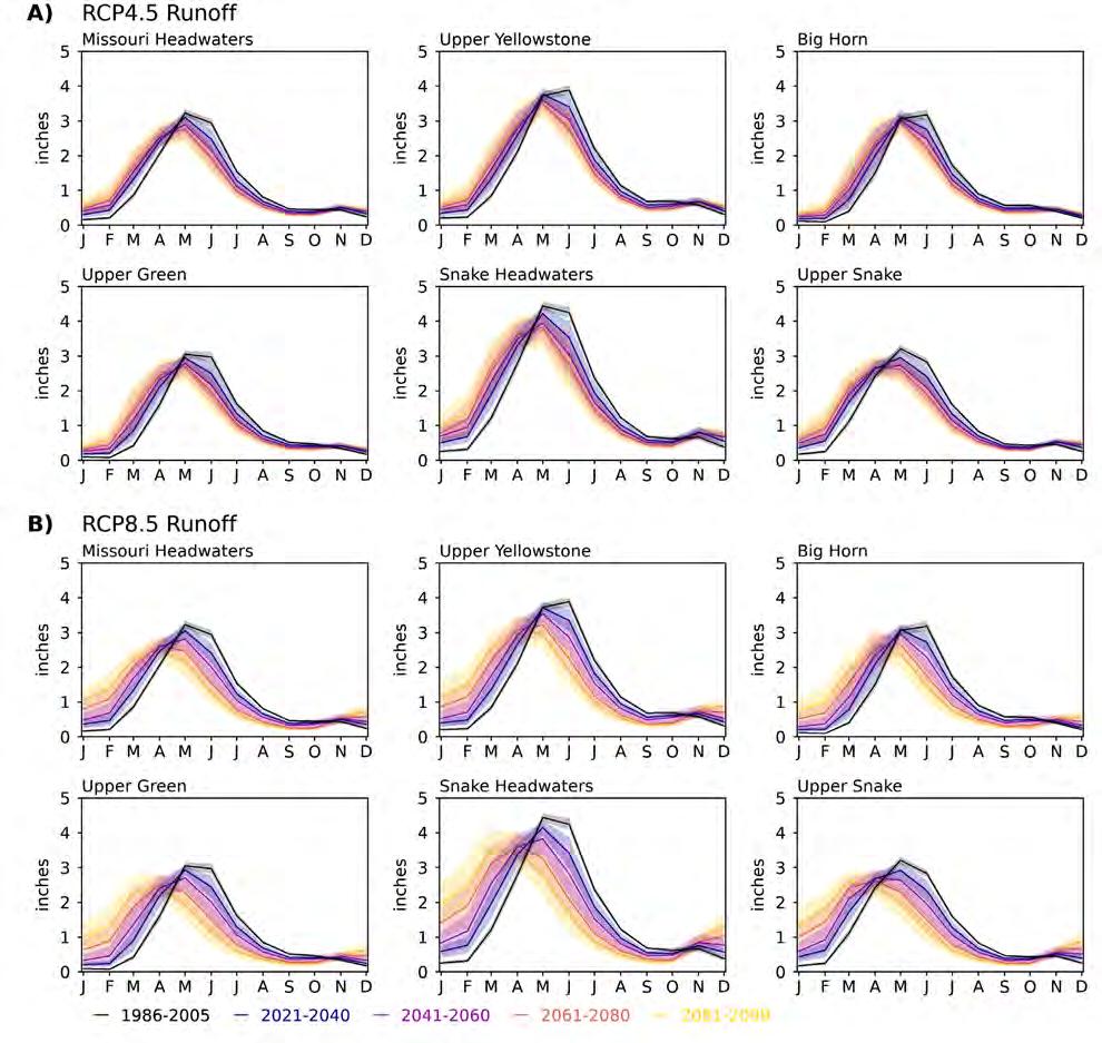
Figure 7-6. Seasonal cycle of mean monthly runoff for the Hydrologic Unit Code 6 (HUC6) watersheds under Representative Concentration Pathway 4.5 (RCP4.5) and RCP8.5, as simulated by the water balance model. The black line shows 1986-2005 base period. The colored lines are the 20-model means of the simulations that used MACAv2-METDATA data as model input for the periods indicated in the legend at the bottom. The shaded bands are the model spread around the respective colored mean lines.

Runoff changes are more striking under RCP8.5 and, except for the Upper Yellowstone and Big Horn watersheds, by the 2061-2080 period peak runoff shifts from May to April. At the end of century peak runoff shifts to March in the southwestern Snake Headwaters and Upper Snake watersheds. Projected summer runoff remains below that of the base period under both RCPs; thus, lower minimum streamflows occur earlier in the year in combination with projected warmer air and likely warmer water temperatures.

Checkerboard plots provide an additional perspective of the changes in projected runoff, model agreement, and the statistical significance of the changes over GYA and HUC6 watersheds (Figure 7-7). As in the checkerboard plots in previous chapters, each rectangular grid in Figure 6-5 illustrates the differences (anomalies) between a given period and the base period (e.g., 20212040 minus 1986-2005) broken down by monthly and annual means, for the GYA and each HUC6 watershed.

Figure 7-7. Change in mean monthly and annual runoff over the Hydrologic Unit Code 6 (HUC6) watersheds and the Greater Yellowstone Area (GYA), as simulated by the water balance model. The columns from left to right show changes for each future period (e.g., 2021-2040) relative to the 19862005 base period with Representative Concentration Pathway 4.5 (RCP4.5) on the top row and RCP8.5 on the bottom row. In each RCP figure, the monthly and annual means (AVG) run from left to right across the horizontal axis on the bottom and the HUC6 watersheds and GYA run along the vertical axis on the left. Colored cells indicate >80% (more than 16 of the 20 models) agree on the sign of the change in the median value (positive or negative). A slash in a colored cell indicates that 60-80% of the models (12-16 out of 20) agree on the sign of the change, and an X in a box indicates that fewer than 60% (<12) of the models agree on the sign of the change. A black dot in a box indicates that the ensemble mean value of the future change is greater than the inter-model standard deviation (SNR >1), an indicator of significance of the change (see Chapter 1 for details). Shown are the 20-model means of the simulations that use the MACAv2-METDATA data.

The progressive shift toward increased late winter and early spring runoff and reduced summer runoff in all HUC6 watersheds is clear across the rows as the century progresses. There is increasingly high model agreement with SNRs >1. This shift is most evident in the Snake Headwaters watershed. Minimal change is projected (i.e., plot colors remain close to white) after September when projected runoff is generally similar to that of the base period.

The link between changes in the timing of snowmelt and runoff in the HUC6 watersheds (Figure 7-3) is highlighted in Figure 7-7. Except for November and December, after 2021-2040, there is high and increasing model agreement and SNRs >1 in the monthly changes over all watersheds.

EvApOTRANSpIRATION ANd SOIL WATER

As discussed in Chapters 2 and 3, drought is a recurring hydrologic feature of the GYA. Like much of the western United States, with future warming drought in the GYA will likely become more frequent and severe. Predicting hydrologic drought and seasonal availability of water in snowdominated areas will become increasingly more challenging as less precipitation falls as snow, snowpack declines, and evapotranspiration increases (Livneh and Badger 2020).

For the 1986-2005 base period, over the GYA mean annual potential evapotranspiration (15.5 inches (39.4 cm)/yr) is greater than actual evapotranspiration (11.7 inches (29.7 cm)/yr) by 3.8 inches (9.6 cm)/yr (Table 7-2). The difference indicates that in the GYA the supply of water from precipitation is insufficient to meet evapotranspiration demand during summer and fall when demand is highest. Additional water is supplied by soil moisture; however, extracting water from the soil gets increasingly more difficult as the soil dries out, both in nature and in the water balance model.

As shown by the seasonal maps for the 1986-2005 base period (left column, Figure 7-8), precipitation minus potential evapotranspiration (P-PET) is positive—that is, precipitation exceeds potential evapotranspiration—over most of the GYA during winter, spring, and fall so there is no water deficit then. Negative values of P-PET, or water deficits, emerge in late spring and persist through summer while PET exceeds P. Negative values indicate how much additional precipitation is needed to balance PET. The largest deficits occur over the lower elevations just outside GYA and in the river valleys and lower elevations within the GYA. P-PET values remain nearly balanced (P equals PET) or slightly positive at higher elevations.

Winter P-PET under RCP4.5 is slightly greater (by about 2%) than winter P-PET of the 1986-2005 base period throughout the 21st century (Figure 7-8) due to increasing precipitation (Figure 6-1). Increasing PET during spring and summer, coupled with little or no change in precipitation, offset winter increases, resulting in progressively lower annual total P-PET values (Table 7-2). GYA-wide, P-PET decreases by 13% annually during the 2021-2040 period and by 19% at the end of century (2080-2099, Table 7-2). Under RCP8.5, annual P-PET is reduced by 18% during the 2041-2060 (Figure A7-3) and by 30% at the end of century (Table 7-2).

Figure 7-8. Seasonal mean precipitation minus potential evapotranspiration (P-PET) in the Greater Yellowstone Area for the 1986-2005 base period (left column), changes under Representative Concentration Pathway 4.5 (RCP4.5, four center columns), and changes at the end of the 21st century under RCP8.5 (right column), as simulated by the water balance model. The seasons (e.g., December-February [DJF]) are arranged in rows and the changes relative to the 1986-2005 base period for each future period (e.g., 20212040) are in columns. Shown are the 20-model means of the simulations that used MACAv2-METDATA data as model input. See Figure A7.3 for RCP8.5.

Like much of the West, the seasonal cycle of P-PET over the HUC6 watersheds is characterized by positive values from October through May and negative values (water deficits) from June through September; July is the most negative month (Figure 7-9). Total annual P-PET for the 1986-2005 base period ranges from 8 inches (20 cm) in the Upper Green to 16 inches (40 cm) in the Snake Headwaters watersheds. Summer (June through September total) deficits for the 1986-2005 base period range from 4 inches (10 cm) in the Upper Yellowstone to 8 inches (20 cm) in the Upper Snake watersheds (Table 7-3). Under both RCPs, through the 21st century summer deficits increase (Table 7-3). Under RCP4.5, by mid century (2041 2060) the increased deficits range from 16% in the Upper Snake to 39% in the Upper Yellowstone watersheds. By the end of the century (2081-2099), deficit increases range from 25% to 53% in those watersheds. Under RCP8.5, deficits increase from 24% in the Upper Snake to 51% in the Upper Yellowstone by mid century and from 54% to 114% in those watersheds by the end of the century.

Note that the graphs in Figure 7-9 are means over the HUCs and summer P-PET over lower elevation agricultural areas can be more negative than the HUC-wide mean depending on location, soils, and use (e.g., alfalfa or pasture). Conversely, at higher elevations, P PET is less negative to slightly positive (Figure 7-8).

Figure 7-9. The seasonal cycle of mean monthly precipitation minus potential evapotranspiration (P-PET) for the Hydrologic Unit Code 6 (HUC6) watersheds under Representative Concentration Pathway 4.5 (RCP4.5) and RCP8.5, as simulated by the water balance model. The black line is shows 1986-2005 base period. The colored lines are the 20-model means of the simulations that used MACAv2-METDATA data as model input for the periods indicated in the legend at the bottom. The shaded bands are the model spread around the respective colored mean lines.

Table 7-3. June through September total precipitation minus potential evapotranspiration (P-PET) in the Hydrologic Unit Code 6 (HUC6) watersheds for the 1986-2005 base period and change during the four future periods under Representative Concentration Pathway 4.5 (RCP4.5) and RCP8.5. The units are in inches and the parenthetical values are percent change. Negative values indicate water deficits, e.g., a value of -6.9 is a deficit of 6.9.

In response to the seasonal cycle of P-PET, soil moisture is recharged during months when P exceeds PET and is depleted during months when PET exceeds P (Figure 7-10). The most negative P-PET occurs in July and minimum soil moisture levels occur in August. Much of the GYA is at or near 100% capacity during spring (MAM, 1986-2005 base period, left column of Figure 7-10), so precipitation and snowmelt become runoff. During summer (JJA) and fall (SON), soil moisture levels fall to about 25% in river basins at lower elevations and remain at 50% and higher over high elevations, reflecting higher precipitation and lower PET there. Beginning in the 2021-2040 period, soil moisture levels are progressively depleted through the century in the lower elevation river basins during spring. Summer and fall soil moisture are progressively lower throughout the GYA, with the largest changes at high elevations where base period moisture levels are higher. These changes are greater under RCP8.5.

Figure 7-10. Seasonal mean soil moisture saturation in the Greater Yellowstone Area for the 1986-2005 base period (left column), changes under Representative Concentration Pathway 4.5 (RCP4.5, four center columns), and changes at the end of the 21st century under RCP8.5 (right column), as simulated by the water balance model. The values are expressed as percentages relative to full water-holding capacity (100%) of the 1-m (39.4-inch) soil layer used in the model (see appendix to this chapter for further details). The seasons (e.g., December-February [DJF]) are arranged in rows and the changes relative to the 1986-2005 base period for each future period (e.g., 2021-2040) are in columns. Shown are the 20-model means of the simulations that used MACAv2-METDATA data as model input. See Figure A7.4 for RCP8.5.

The checkerboard plot (Figure 7-11) shows the emerging seasonal change of soil water in the HUC6 watersheds and GYA through the 21st century. As in previous figures, each rectangular grid in Figure 7-11 illustrates the differences (anomalies) between a given period and the base period (e.g., 2021-2040 minus 1986-2005) broken down by monthly and annual means, for the GYA and each HUC6 watershed.

Winter increases are accompanied by summer decreases. The largest decreases occur in May through July and again in October when increased evapotranspiration extracts more soil moisture. The smaller relative changes in August and September reflect the limitation on how much water can be extracted from the already dry soil in the 1986-2005 base period.

Figure 7-11. Change in monthly and annual mean soil moisture saturation over the Hydrologic Unit Code 6 (HUC6) watersheds and Greater Yellowstone Area (GYA), as simulated by the water balance model. The values are expressed as percentages relative to full water-holding capacity (100%) of the 1-m (39.4-inch) soil layer used in the model (see appendix to this chapter for further details). The columns from left to right show changes for each future period (e.g., 2021-2040) relative to the 1986-2005 base period with Representative Concentration Pathway 4.5 (RCP4.5) on the top row and RCP8.5 on the bottom row. In each RCP figure, the months and annual mean (AVG) run from left to right across the horizontal axis on the bottom and the HUC6 watersheds and GYA run along the vertical axis on the left. Colored cells indicate >80% (more than 16 of the 20 models) agree on the sign of the change in the median value (positive or negative). A slash in a colored cell indicates that 60-80% of the models (12-16 out of 20) agree on the sign of the change, and an X in a box indicates that fewer than 60% (<12) of the models agree on the sign of the change. A black dot in a box indicates that the ensemble mean value of the future change is greater than the inter-model standard deviation (SNR >1), an indicator of significance of the change (see Chapter 1 for details). Shown are the 20-model means of the simulations that used the MACAv2-METDATA data as model input.

The combined projected changes in P-PET and soil moisture content indicate that the magnitude and duration of the today’s summer and fall period of water deficit will be greater in the future. There is a high level of model agreement (>80%) and SNRs >1 for the changes. These projections are based on climatological means over 20-year periods with a range of variability attributed to the 20 climate models used in the Assessment. Shorter-term, more severe drought conditions not captured by the models are likely to occur in the future just as they have in past. Future droughts will occur under warmer average conditions and hence have the potential to be more extreme than those of the past or present.

Future droughts will occur under warmer average conditions and hence have the potential to be more extreme than those of the past or present.

Winter Recreation

GYA is world renowned as a destination for skiing, snowboarding, snowmobiling, ice climbing, dogsledding, ice fishing, and other winter activities (see figure). In the future, these recreational opportunities—and associated economies—will be threatened by the continued loss of snowpack as the GYA snow season becomes shorter and more uncertain.

Winter recreational opportunities, and the associated economies, will be threatened as the climate warms and snowpack is lost. (Photo credits, clockwise from left: Rick and Susie Graetz, Scott Bischke, JMT Photography/Pexels, and Glenn Claire/Upsplash)

Consistent with most of the mountainous western United States, annual snowpack in the GYA is declining. Since 1950, snowfall at an elevation of 8000 ft in the GYA has decreased by 3.5 inches (8.9 cm)/decade (about 25%), so nearly 24 inches (61 cm) less snow now falls annually (see Chapter 3).

Snowpack of the 1990s and early 2000s in the GYA, as measured by snow water equivalent on April 1st, was at least 20% lower than the average of the past 8 centuries (see Chapter 3; Pederson et al. 2011). The observed loss of snowfall and snowpack in the GYA is attributed to warmer temperatures from November through April (Tercek at al. 2015), increased precipitation in spring and fall, and decreased precipitation in winter and summer (see Chapter 3).

Decreases in snowpack are projected to continue in the future (Figures 7.1 and A7.1). As winters warm, a smaller portion of precipitation will fall as snow (Table 7.1) and more precipitation will be a mixture of rain and snow. Under RCP4.5, mid-century loss of snowpack ranges between 24 and 31% of 1986-2005 levels and reaches 38-44% by the end of century (Figure 7.2 and Table 7.1). Losses are much greater under the warmer conditions of RCP8.5.

Elevational changes in snow will affect most aspects of winter recreation in the GYA. In Yellowstone National Park, for example, Tercek and Rodman (2015) found that the length of the snow season at the end of century (20612090) could decline by 16 and 27% over present under RCP4.5 and RCP8.5, respectively, with similar or greater declines in the number of days suitable for over-snow vehicles. Lackner et al. (2021) projected that under RCP8.5 over the 30-year period centered on 2050, the number of ski days during the core of the season will be reduced from 6 to 29 days at ski areas within the GYA.

SuMMARY

Projected snow changes.— Under RCP4.5, the total area of the GYA dominated by winter snowfall decreases from 59% during the base period (1986-2005) to 27% at mid century (2041-2060) and to 11% by the end of century (2081-2099). Under RCP8.5, the extent of snow-dominant area decreases to 17% and to 1% for the same time periods, respectively. There is >80% model agreement and SNR >1 for the changes. The amount of water stored in the snowpack decreases over the GYA and all HUC6 watersheds. The projected loss of water in the snowpack is consistent with previous studies in the region (e.g., Klos et al. 2014; Tennant et al. 2015; Tersek and Rodman 2015; Whitlock et al. 2017; Conant et al. 2018; Alder and Hostetler 2019). The RCP4.5 and RCP8.5 snowpack trajectories mirror those of temperature for the HUC6 watersheds shown in Figure 5-4, illustrating the strong dependence of snowpack on temperature. The snow projections are likely an upper bound on future changes that may occur because the spatial resolution of our water balance model is relatively coarse, and the model does not account for sublimation, wind, and local, non-climatic factors such as slope, aspect, and shading. Such factors influence the rate and distribution of local changes in snow accumulation and snowmelt (e.g., Watson et al. 2008; Pavelsky et al. 2012).

Projected runoff changes.—Under both RCP4.5 and RCP8.5, the amount of total annual runoff increases slightly (from 1 to 3%) through the 21st century in the GYA and HUC6 watersheds. The increases are related to shifting seasonality (Table 7-2). There is varying model agreement by time period (Figure 7-7 and Table 7-2). Under both RCP4.5 and RCP8.5, there is 90-100% model agreement and SNR >1 for the projected shifts in seasonal and monthly runoff during winter, spring, and summer. These findings are consistent with previous studies (Tennant et al. 2015; Whitlock et al. 2017; Alder and Hostetler 2019; Livneh and Badger 2020).

Precipitation minus potential evapotranspiration and water deficit.—Over the GYA and HUC6 watersheds, potential evapotranspiration (PET) demand exceeds precipitation (P) during summer (June through September), leading to water deficits, particularly at lower elevations. Under RCP4.5, the GYA summer water deficit is projected to increase by 25% at mid century and 36% by the end of century. Under RCP8.5, projected water deficit increases are 35% by mid century and 79% by the end of century (Table 7-3). Under RCP4.5, by mid century (2041-2060) summer deficit increases in the HUC6 watersheds range from 16% in the Upper Snake to 39% in the Upper Yellowstone. By the end of the century (2081-2099), the increases range from 25 to 53% in those watersheds. Under RCP8.5, deficit increases range from 24% in the Upper Snake to 51% in the Upper Yellowstone by mid century, and from 54 to 114% in those watersheds by the end of the century.

Soil moisture.— Summer soil moisture levels are about 25% of capacity over low elevations and 50% of capacity at higher elevations of the GYA during the 1986-2005 base period. Under RCP4.5, June-October soil moisture saturation decreases by 23% at mid century and 33% by the end of the century. Under RCP8.5, June-October soil moisture saturation decreases by 30% mid century and by 56% by the end of the century. There is >80% model agreement and SNRs >1 for the changes. These changes in average conditions will likely intensify summer drought in the GYA and HUC6 watersheds.

ChApTER 7 AppENdIx—A dEEpER LOOk

Climate variables

The variables discussed in this chapter are summarized in Table A7-1.

Table A7-1. The climate and water balance variables discussed in this chapter (MWBM is Monthly Water Balance Model).

Variable Description Source Units

Potential Solar radiation

The amount of incoming solar radiation at the surface calculated by day-of-year and latitude independent of cloud cover

Snow or Snow water equivalent (SWE) The amount of water stored in snow.

Runoff

Soil water saturation

Actual evapotranspiration

Potential evapotranspiration

Snow-to-rain ratio

Snowmelt

Depth of excess water available for streamflow and groundwater

Depth of water stored in the 1-m (39.4-inch) soil layer. Here measured as the percent of saturated capacity (100%)

Depth of actual water loss to the atmosphere by combined evaporation from soils and transpiration from plants

The depth of evapotranspiration that would occur with unlimited water availability.

The percent of precipitation falling as snow

The depth of water from melted snow determined by degree-day method

The water balance model

MWBM Watts per meter squared (W m-2)

MWBM Inches Centimeters (cm)

MWBM Inches Centimeters (cm)

MWBM Percent

MWBM Inches Centimeters (cm)

MWBM Inches Centimeters (cm)

MWBM Percent

MWBM Inches Centimeters (cm)

The monthly water balance model accounts for the partitioning of water through the various components of the hydrological system (McCabe and Markstrom 2007). Air temperature determines the portion of precipitation that falls as rain or snow, the accumulation and melting of the snowpack, and actual evapotranspiration. Snowmelt is calculated by a degree-day method and potential evapotranspiration is determined from temperature and potential solar radiation by the Oudin method (Oudin et al. 2005). Rain and melting snow are partitioned into direct surface runoff, soil moisture, and surplus runoff that occurs when the soil layer reaches 100% saturation. The soil layer has a 1-m (39.4-inch) rooting depth and spatially variable water holding capacity derived from the State Soil Geographic Data Base (viger and Bock 2014; Schwarz and Alexander 1995; Wolock 1997).

The model has been applied to climate-hydrology studies (e.g., Wolock and McCabe 1999; McCabe and Wolock 2011a,b; McCabe et al. 2013) including the GYA (Gray and McCabe 2010; Pederson et al. 2013; Hostetler and Alder 2016; Alder and Hostetler 2019; Battaglin et al. 2020). The model is also used to provide CMIP5 climate change and hydrological data for the conterminous United States (https://doi.org/10.5066/F7W9575T). Computer code for implementing a default version of the model is available from the National Center for Atmospheric Research (https://www.ncl.ucar. edu/Applications/crop.shtml, accessed February 2021).

Some details of the model include:

о the model is run on a monthly time step, so it does not capture day-to-day variability nor extreme events such as intense precipitation and floods;

о surface elevation is implicit through the MACAv2-METDATA temperature and precipitation data, but the model does not account for detail of slope or aspect below the resolution of the 4 km by 4-km (2.5-mile by 2.5-mile) grid cells used in the Assessment;

о while physically based, the model simplifies more complex energy balance details that determine evapotranspiration and snow dynamics; and

о the model simulates the runoff of a grid cell but does not route runoff among grid cells or into stream networks or groundwater.

Accordingly, for the Greater Yellowstone Climate Assessment the model is intended to provide a reasonable estimate of hydrologic change over the 21st century. More detailed analyses in the next phase of the GYA Assessment, such as modeling potentially complex local changes in snow, streamflow and groundwater and their interaction, will require more detailed representations of the underlying processes and calibration in catchments.

Figures supporting Chapter 7

Details of Figures 7-1 and A7-1 snow graphics.—In Figures 7-1 and A7-1, we map and plot the unitless ratio of the maximum amount of water stored in the snow (i.e., the snowpack) from October through April, which is referred to as the snow water equivalent (SWE), to total precipitation (P) over the same period, SWE:P. The ratio implicitly accounts for changes in precipitation and temperature on snow accumulation (Serreze et al. 1999; Mantua et al. 2010; Sproles et al. 2017). As shown in the color bars at the bottom of the figures, we follow Mantua et al. (2010) in specifying three zones of the ratio, which in GYA are related to elevation:

1 rain-dominated, where most precipitation falls as rain (SWE:P values < 0.1, green in the figures);

2 rain-snow mix, where precipitation falls as a mix of rain and snow (0.1 ≤ SWE:P < 0.4, orange and red colors in the figures) with the lowest range indicating more rain and the highest range more snow; and

3 snow-dominant zone (SWE:P ≥ 0.4, blue colors in the figures), where most precipitation falls as snow.

Figure A7-1. The 1986-2099 annual snow regime for the Hydrologic Unit Code 6 (HUC6) watersheds under Representative Concentration Pathway 8.5 (RCP8.5), as simulated by the water balance model. The five maps across the top display the ratio of maximum snow water equivalent (SWE) to total cold-season (Oct-Apr) precipitation (P) SWE:P for the indicated time periods. The pie charts inset in the maps show the fraction of Greater Yellowstone Area (GYA) area within each SWE:P category. The time-elevation plots for the HUC6 watersheds in the bottom two rows display the trend in SWE:P ratio from 1986-2099 averaged over 330 ft (100 m) elevation bands. Gray shading indicates elevations not present in the HUCs.

Figure A7-2. Seasonal mean runoff in the Greater Yellowstone Area for the 1986-2005 base period (left column), changes under Representative Concentration Pathway 8.5 (RCP8.5, four center columns), and changes at the end of the 21st century under RCP4.5 (right column), as simulated by the water balance model. The seasons (e.g., December-February [DJF]) are arranged in rows and the changes relative to the 1986-2005 base period for each future period (e.g., 2021-2040) are in columns. Shown are the 20-model means of the simulations that used MACAv2-METDATA data as model input.

Figure A7-3. Seasonal mean precipitation minus potential evapotranspiration (P-PET) in the Greater Yellowstone Area for the 1986-2005 base period (left column), changes under Representative Concentration Pathway 8.5 (RCP8.5, four center columns), and changes at the end of the 21st century under RCP4.5 (right column), as simulated by the water balance mode. The seasons (e.g., December-February [DJF]) are arranged in rows and the changes relative to the 1986-2005 base period average period for each future period (e.g., 2021-2040) are in columns. Shown are the 20-model means of the simulations that used MACAv2-METDATA data as model input.

Figure A7-4. Seasonal mean soil moisture saturation in the Greater Yellowstone Area for the 1986-2005 base period (left column), changes under Representative Concentration Pathway 8.5 (RCP8.5, four center columns), and changes at the end of the 21st century under RCP4.5 (right column), as simulated by the water balance model. The values are expressed as percentages relative to full water-holding capacity (100%) of the 1-m (39.4-inch) soil layer used in the model. The seasons (e.g., December-February [DJF]) are arranged in rows and the changes relative to the 1986-2005 base period for each future period (e.g., 20212040) are in columns. Shown are the 20-model means of the simulations that used MACAv2-METDATA data as model input.

LITERATuRE CITEd

Alder JR, Hostetler SW. 2019. The dependence of hydroclimate projections in snow‐dominated regions of the western United States on the choice of statistically downscaled climate data. Water Resources Research 55(3)2279-300. https://doi.org/10.1029/2018WR023458.

Battaglin W, Hay L, Lawrence DJ, McCabe G, Norton P. 2020. Baseline conditions and projected future hydroclimatic change in national parks in the conterminous United States. Water 12(6):1704. doi:10.3390/ w12061704.

Conant RT, Kluck D, Anderson M, Badger A, Boustead BM, Derner J, Farris L, Hayes M, Livneh B, McNeeley S, Peck D, Shulski M, Small v. 2018. Northern Great Plains [chapter 22]. In: Impacts, Risks, and Adaptation in the United States: Fourth National Climate Assessment, vol II. In: Reidmiller DR, Avery CW, Easterling DR, Kunkel KE, Lewis KLM, Maycock TK, Stewart BC, editors. Washington DC: US Global Change Research Program. p 941-86. https://doi.org/10.7930/NCA4.2018.CH22.

Gray ST, McCabe GJ. 2010. A combined water balance and tree ring approach to understanding the potential hydrologic effects of climate change in the central Rocky Mountain region. Water Resources Research 46(5). doi:10.1029/2008wr007650.

Hostetler SW, Alder JR. 2016. Implementation and evaluation of a monthly water balance model over the US on an 800-m grid. Water Resources Research 52(12):9600-20. doi:10.1002/2016WR018665

Klos PZ, Link TE, Abatzoglou JT. 2014. Extent of the rain-snow transition zone in the western US under historic and projected climate. Geophysical Research Letters 41:4560-8.

Lackner CP, Greets B, Wang Y. 2021 (Mar 19). Impact of global warming on snow in ski areas: a case study using a regional climate simulation over the interior western United States Journal of Applied Meteorology and Climatology. Available online only. doi:10.1175/JAMC-D-20-0155.1.

Li DY, Wrzesien ML, Durand M, Adam J, Lettenmaier DP. 2017. How much runoff originates as snow in the western United States, and how will that change in the future? Geophysical Research Letters 44:6163-72.

Livneh B, Badger AM. 2020. Drought less predictable under declining future snowpack. Nature Climate Change 10:452-8.

Mantua N, Tohver I, Hamlet A. 2010. Climate change impacts on streamflow extremes and summertime stream temperature and their possible consequences for freshwater salmon habitat in Washington State. Climatic Change 102:187-223.

McCabe GJ, Betancourt JL, Pederson GT, Schwartz MD. 2013. variability common to first leaf dates and snowpack in the western conterminous United States. Earth Interact 17(26):1-18. doi:10.1175/2013ei000549.

McCabe GJ, Markstrom SL. 2007. A monthly water-balance model driven by a graphical user interface. US Geological Survey open-file report 2007-1088. Reston vA: USGS. 12 p. Available online https://pubs.usgs. gov/of/2007/1088/pdf/of07-1088_508.pdf. Accessed 10 Mar2021.

McCabe GJ, Wolock DM. 2011a. Independent effects of temperature and precipitation on modeled runoff in the conterminous United States. Water Resources Research 47(11). https://doi. org/10.1029/2011WR010630.

McCabe GJ, Wolock DM. 2011b. Century-scale variability in global annual runoff examined using a water balance model. International Journal of Climatology 31(12):1739-48. https://doi.org/10.1002/joc.2198.

McCabe GJ, Wolock DM. 2015. variability and trends in global drought. Earth and Space Science 2(6):223-8. doi:10.1002/2015ea000100.

Musselman KN, Lehner F, Ikeda K, Clark MP, Prein AF, Liu C, Barlage M, Rasmussen R. 2018. Projected increases and shifts in rain-on-snow flood risk over western North America. Nature Climate Change 8:808-12. https://doi.org/10.1038/s41558-018-0236-4.

[NOAA-NCEI] National Oceanic and Atmospheric Administration-National Centers for Environmental Information. [undated]. Drought—June 2012 [webpage]. Available online https://www.ncdc.noaa.gov/ sotc/drought/201206. Accessed Feb 2021.

Oudin L, Hervieu F, Michel C, Perrin C, Andréassian v, Anctil F, Loumagne C. 2005. Which potential evapotranspiration input for a lumped rainfall-runoff model? Part 2 – Towards a simple and efficient potential evapotranspiration model for rainfall-runoff modelling. Journal of Hydrology 303(1-4):290-306.

Pavelsky TM, Sobolowski S, Kapnick SB, Barnes JB. 2012. Changes in orographic precipitation patterns caused by a shift from snow to rain. Geophysical Research Letters 39(18). https://doi. org/10.1029/2012GL052741.

Pederson GT, Betancourt JL, McCabe GJ. 2013. Regional patterns and proximal causes of the recent snowpack decline in the Rocky Mountains, US. Geophysical Research Letters 40(9):1811-6. doi:10.1002/ Grl.50424.

Pederson GT, Gray ST, Woodhouse CA, Betancourt JL, Fagre DB, Littell JS, Watson E, Luckman BH, Graumlich LJ. 2011. The unusual nature of recent snowpack declines in the North American Cordillera. Science 333:332-5.

Queen LE, Mote PW, Rupp DE, Chegwidden O, Nijssen B. 2021. Ubiquitous increases in flood magnitude in the Columbia River basin under climate change. Hydrology and Earth System Science 25(1):257-72. doi:10.5194/hess-25-257-2021.

Schwarz GE, Alexander RB. 1995. State Soil Geographic (STATSGO) data base for the conterminous United States. US Geological Survey open-file report 95-449. Reston vA: USGS. doi:10.3133/ofr95449.

Serreze MC, Clark MP, Armstrong RL, McGinnis DA, Pulwarty RS. 1999. Characteristics of the western United States snowpack from snowpack telemetry (SNOTEL) data. Water Resources Research 35(7):2145-60. https://doi.org/10.1029/1999WR900090.

Sproles EA, Roth TR, Nolin AW. 2017. Future snow? A spatial-probabilistic assessment of the extraordinarily low snowpacks of 2014 and 2015 in the Oregon Cascades. The Cryosphere 11:331-41. https://doi. org/10.5194/tc-11-331-2017.

Tennant CJ, Crosby BT, Godsey SE. 2015. Elevation-dependent responses of streamflow to climate warming. Hydrological Processes 29(6):991-1001. doi:10.1002/hyp.10203

Tercek MT, Rodman AW. 2015. Forecasts of 21st-century snowpack and implications for snowmobile and snowcoach use in Yellowstone National Park. PLOS One 11. https://doi.org/10.1371/journal. pone.0159218.

Tercek MT, Rodman AW, Thoma D. 2015. Trends in Yellowstone snowpack. Yellowstone Science 23(1):20-7. viger RJ, Bock AR. 2014. GIS features of the geospatial fabric for national hydrologic modeling [webpage]. US Geological Survey data source. Available online https://data.usgs.gov/datacatalog/data/ USGS:581a11f0e4b0bb36a4ca2dfc. Accessed 10 Mar 2021 doi:10.5066/F7542KMD

Watson FGR, Anderson TN, Newman WB, Cornish SS, Thein TR. 2008. The ecology of large mammals in central Yellowstone: sixteen years of integrated field studies, vol 3. P 85-112. Cambridge MA: Academic Press. doi:10.1016/S1936-7961(08)00206-6.

Whitlock C, Cross W, Maxwell B, Silverman N, Wade AA. 2017. 2017 Montana Climate Assessment. Bozeman and Missoula MT: Montana State University and University of Montana, Montana Institute on Ecosystems. 318 p. doi:10.15788/m2ww8w.

Wolock DM. 1997. STATSGO soil characteristics for the conterminous United States. US Geologic Survey open-file report 97-656. Reston vA: USGS. doi:10.3133/ofr97656.

Wolock D, McCabe G. 1999. Explaining spatial variability in mean annual runoff in the conterminous United States. Climate Research 11:149-59.

8. VOICES FROM THE GREATER YELLOWSTONE AREA

Charles Wolf Drimal, Ryan Cruz, Allison Michalski, and Emily Reed

kEY MESSAGES

о Water issues are at the core of climate change impacts in the GYA. Communities and environmental managers will continue to face challenges like drought and shifts in seasonal water cycles in the future.

о Participants’ understanding of and response to climate change is driven more by their background (stakeholder group) than their location (watershed).

о A pressing need exists for a climate information hub that is comprehensive, collaborative, accessible, and useful to experts and the public alike.

о For the most part, meaningful policy to address and adapt to climate change is lacking in the GYA.

о By addressing water issues like availability and quality in future climate adaptation work, we stand to have positive impacts on myriad other conditions including wildlife habitat, fisheries health, and the economy of local communities.

Looking out over the Gravelly Range, Upper Missouri Headwaters, Montana Photo courtesy of Rick and Susie Graetz

INTROduCTION

The Greater Yellowstone Area is home to a great diversity of species and environments and a rich variety of cultures. Our communities have different perspectives on climate issues, as well as different approaches to climate adaptation and resilience work. As we work to better understand how climate change will affect the region, continuous engagement with stakeholders and knowledge of their realities in dealing with climate change can improve effectiveness of GYA science, monitoring, and adaptation.

This chapter speaks to people’s stories and experiences. We recognize that climate change research requires input from multiple disciplines including those of the social sciences. Public opinion and human action play an integral role in ecological management. Our intention is to provide insight for professionals working on climate adaptation and resiliency projects so that they may better integrate community needs into their work. We also hope that the perspectives represented here, coupled with future public meetings in all six watersheds of the GYA, will set the stage for collaborative action among community, agency, and Tribal members that addresses climate adaptation and resilience on a large-landscape scale.

[C]ontinuous engagement with stakeholders and knowledge of their realities in dealing with climate change can improve effectiveness of GYA science, monitoring, and adaptation.

Keeping this in mind, we conducted one-onone listening sessions with 44 community leaders, city officials, agency biologists, business owners, engaged citizens, and ranchers (Figure 8-1). We chose these participants to get as many diverse perspectives as possible, using existing relationships and reaching out to new individuals. Interviews were conducted remotely either by phone or video, transcribed, then coded and analyzed by a team from The Greater Yellowstone Coalition, The Wilderness Society, and the University of Wyoming during spring, summer, and fall of 2020. Participants were spread across the six HUC6 watersheds discussed in previous chapters (Figure 8-1; descriptions in Chapter 1): Missouri Headwaters, Upper Yellowstone, Big Horn, Upper Green, Upper Snake, and Snake Headwaters.

To understand how different people and communities view issues related to environmental and climate change, we grouped our participants into six stakeholder groups as described in Table 8-1.

We note two qualifiers to results presented in this chapter. First, we did not have a statistically significant sample size of all stakeholder types throughout the region, nor did we have an equal number of interviews for each type. Thus, our ability to conduct statistical analysis across different watersheds and stakeholder categories—which would have been ideal—was limited. The results presented in this chapter are based on qualitative thematic coding. Our qualitative research interviews with stakeholders coincided with the unfolding of the Covid-19 pandemic, which presented a host of challenges both for interviewers and interviewees. Second, the trends we have identified are not absolute and may not be representative of what all members of a given group experience, believe, or do. Nonetheless, these participant responses provide important insights into the concerns of individuals and communities within the GYA and underscores the need for more social science research on climate change.

Figure 8-1. Map of the Greater Yellowstone Area (GYA) showing the six Hydrologic Unit Code 6 (HUC6) watersheds studied under the Assessment, and including mountain ranges, lakes and major river systems, jurisdictions, and selected towns. The portions of the watersheds within the GYA boundary are studied in this report (see Chapter 1 for descriptions of each watershed). The number of interviewees from each watershed is shown in the blue. (Map created using ArcGIS® software, copyright ESRI and used herein under license.)

Table 8-1. The 44 interviews conducted included six stakeholder groups.

from a combination of locally focused entities like county planners, water district staff, and the energy industry

owners that are involved in tourism or outdoor recreation (e.g., ski resorts, outfitters, and lodging)

of Apsáalooke/Crow and Shoshone-Bannock Tribes with an intimate understanding of their communities’ needs, as well as the longterm state of the landscape

In this chapter, we summarize stakeholder opinions on the topics of environment and climate change, with related responses sorted into seven categories:

о Stakeholder concerns

о Impacts to stakeholders

о Current information

о Information needed

о Leaders and current work

о Project needs

о Policy

STAkEhOLdER CONCERNS

We asked participants: What worries you the most about projected uncertainty in environmental factors such as temperature, drought, water availability, runoff, soil moisture, fire, or seasonal patterns and climate?

Our first question gave us insight into the issues most concerning to our participants. Our goal was to better understand how different people think about the challenge of climate change. In some cases, these issues may not, to date, have been observed.

Concerns among stakeholder groups

Overall, concerns about water were expressed the most. various water issues were mentioned in over half of the interviews for every stakeholder group, ranging from just over half of Recreation interviews to all interviews from Tribal members and Local Government/Utilities. Issues like shifts in peak runoff timing and extreme flooding were the main concern for Agency and Conservation stakeholders, while issues of water supply rose to the top for Local Government/ Utilities participants. Agriculture producers and Tribal members were equally concerned about the possibility of shifting hydrological events and loss of water supply. Concerns about water quality and temperature were also expressed, although less frequently (Figure 8-2).

“We conducted a survey with all of our 850 rural families and their biggest concern is water. Water is a big concern for everybody.”

— Tribal MeMber, Upper YellowsTone waTershed

“I think drought is the biggest threat to everything we value in Montana.”

— ConservaTionisT, MissoUri headwaTers waTershed

Recreation was the only stakeholder group that mentioned another concern more often than water. Though they still mentioned water in most interviews, these stakeholders were more worried about habitat. This concern may reflect the role that healthy habitats play in many forms of outdoor recreation, including fishing, hiking, hunting, and wildlife watching. Unsurprisingly, Recreation stakeholders were also especially concerned about the impacts of climate change to outdoor recreation.

Local Government/Utility participants were the only other group notably concerned about outdoor recreation, which likely reflects the importance of recreation and tourism economies for many GYA communities. A Local Government/ Utility participant working in the Missouri Headwaters watershed explained, “We are a ski resort community, and that is the life blood of what our community thrives on and our local economy.”

Figure 8-2. A word cloud showing the factors that participants expressed concerns about in relation to changing environmental conditions and climate. Word size corresponds with the prevalence of the concern mentioned in interviews, with common concerns shown larger.

Agriculture producers stood out in expressing their concerns about the public’s limited awareness of climate change. They also made explicit mention of having few or no concerns themselves. While these two responses may sound contradictory, many agriculturalists pointed out that producers have always adapted to changing and unpredictable climate conditions. In their view, they will simply continue to do so, even as the climate changes. As one agricultural producer in the Missouri Headwaters put it, they have been adapting “forever on a daily basis” by making decisions about which crops to plant, how and when to irrigate, and more. Expressing a lack of concern does not necessarily mean that Agriculture participants deny that the climate is changing or that there will not be consequences.

“If you’re in agriculture, the key thing is that you are experiencing changes every day. It’s not like this is something like, ‘Oh we have climate change now!’

You’ve been dealing with this on a daily basis.”

— agriCUlTUral prodUCer, MissoUri headwaTers waTershed

Many participants were concerned about the impact of climate change on the region’s communities. Specific concerns included increased wildfire risk, threats to infrastructure, and unsustainable water usage. Concerns about the health of fish and wildlife were also expressed, including climate-triggered fish kills and wildlife population declines. Local Government/Utility and Agriculture participants were most concerned about the effects of climate change on communities, while Conservation and Agency groups more often mentioned threats to fish and wildlife. Tribal and Recreation participants were equally concerned about both topics.

Concerns within watersheds

When we looked at how responses differed among watersheds instead of stakeholder groups, we found similarities. Water-related concerns were paramount in all areas, particularly in the Upper Yellowstone and Missouri Headwaters watersheds where participants specifically expressed concern about declines in water supply. These watersheds are home to the rapidly growing communities of Bozeman and Livingston, Montana, where water demand is on the rise.

Other concerns were strikingly consistent across all watersheds. For example, changes in hydrological events like flooding and peak runoff were raised by two thirds of participants in all areas. Potential climate change impacts to habitat, wildfire, and communities were also mentioned consistently across watersheds. These concerns were widely shared across the GYA, even though stakeholder groups prioritized them differently.

[C]hanges in hydrological events like flooding and peak runoff were raised by two thirds of participants in all areas. Potential climate change impacts to habitat, wildfire, and communities were also mentioned consistently across watersheds.

Concerns about about fish and wildlife, on the other hand, varied dramatically among watersheds, even adjacent ones. For example, participants from the Upper Yellowstone watershed mentioned these concerns in almost three quarters of interviews, yet it never came up in interviews from the Missouri Headwaters watershed. In contrast, every stakeholder in the Snake Headwaters watershed mentioned concerns about the health of fish and wildlife. Sport and native fisheries

Release of the Madison River from Ennis Lake dam and powerhouse near Ennis, Montana

Photo courtesy of Scott Bischke

IMpACTS TO STAkEhOLdERS

We asked participants: Are changes in environmental factors, seasonal patterns, and climate impacting you and your work today, and if so, how?

Our second question built on the first, by diving deeper into how climate change is currently affecting stakeholders. Their responses illustrate how people from different sectors perceive and experience current conditions.

Impacts on stakeholder groups

All stakeholder groups mentioned water-related impacts more often than any other kind of impact (Figure 8-3). Their collective focus on water impacts was even more prevalent than their concern about future changes in water resources. References to water impacts varied, with all Tribal and Local Government/Utility participants mentioning the issue, while just over half of Conservation and Agency participants did so. Changes in extreme hydrological events, particularly changes in peak runoff and the occurrence of floods, were of paramount concern for all stakeholder groups. This response suggests that recent short-term events stand out in the minds of the participants more than more gradual changes in water supply.

Figure 8-3. A word cloud showing the factors that participants have observed being already impacted as a result of changing environmental conditions and climate today. Word size corresponds with the prevalence of the impact mentioned in interviews, with common impacts shown larger.

Many participants also noted that these extreme hydrological events ultimately have myriad consequences. A Recreation participant from the Upper Yellowstone watershed related rapid spring runoff to water supply and quality issues, saying, “Even when we do get a good amount of snow, it’s going to come out earlier and faster, leaving us with difficult water conditions in late summer especially.” An Agency participant from the same area noted the effect of spring flooding on habitat, explaining, “There is some information to suggest that, with runoff happening earlier and all at once, that can cause an increased impact on stream channel instability... which has implications for fish habitat.”

Asking about observed impacts also shed light on Agriculture’s lower concern for the future, noted in the previous summary. Three quarters of agriculture participants stated that current changes in climate were not altogether unusual and dealing with them was a routine part of their work. It is not that Agriculture participants fail to see changing conditions, but rather, they have always had to respond to them in one way or another.

Changes in extreme hydrological events, particularly changes in peak runoff and the occurrence of floods, were of paramount concern for all stakeholder groups. This response suggests that short-term events stand out in the minds of the participants more than more gradual changes in water supply.

In terms of the other ecological impacts, the increase of wildfire and rising air temperatures were mentioned by all stakeholder groups, though not in a prominent way. Impacts to fish and wildlife also came up in interviews from all groups, particularly those from Agency or Tribal participants, and impacts to aquatic species were most common.

Observations of current climate change impacts on local communities were mentioned often by all stakeholder groups except Agriculture and Recreation participants. The finding is interesting, considering that all stakeholder groups—including Agriculture and Recreation—expressed community-related concerns for the future. This discrepancy suggests that, while people of all walks of life recognize the threats facing our communities, some stakeholders are in a better position than others to directly witness those changes today.

“Used to be more often than not you’d have the water in the reservoirs. More often than not now we don’t. It’s gotten really unreliable.”

Above Boulder Lake (reservoir) near Pinedale WY in the upper Green River watershed

Photo courtesy of Scott Bischke

Reported community impacts included infrastructure damages from wildfires and flooding, as well as growing demand for water or power. Some participants attributed these impacts to changing environmental conditions. An agency member from the Upper Snake watershed, for example, said, “In 2012 we experienced a small-time disaster here in the area in this region in relation to wildfire, in the Charlotte Fire, that destroyed 60 homes. And while that wasn’t unique in the Intermountain West in 2012, the frequency of those happening seems to be on the rise.”

Other participants highlighted how these issues sometimes are the result of unsustainable land use, including urban sprawl and the development of rural areas. A Local Government/Utility participant in the Upper Yellowstone watershed explained, “Our funding model is not designed to provide services to all parts of the county, and yet we’re being asked to do just that.”

Impacts on watersheds

Accounts of climate change showed some similarities across watersheds. Again, stakeholders cited changes in water factors the most, with observations of extreme hydrological events in all areas. Stakeholders mentioned wildfire impacts in all watersheds, as well, though less frequently than water factors.

Conversely, stakeholders mentioned seeing habitat changes and impacts to communities today in only a few watersheds despite expressing widespread worries on these factors for the future, as mentioned previously. Similarly, observed impacts to fish and wildlife varied between watersheds, in contrast to the general concern in all areas about the health of species in the future. Nearly three quarters of interviewees in the Upper Yellowstone watershed noted changes in fish and wildlife health, whereas participants in the Upper Green watershed described no current impacts.

Photos courtesy of Scott Bischke (swans at Harriman State Park, in Idaho) and Pixabay/Pexels (fire).

CuRRENT INFORMATION

We asked participants: What are your current sources of information in the Greater Yellowstone Area on environmental factors, seasonal patterns, and climate?

After participants conveyed to us their concerns about environmental change (including those associated with climate change) and the impacts that they have already observed, we wanted to find out where they got their information. Their answers may explain why particular environmental issues are relevant for a given group, helping us develop more effective distribution of environmental and climate change information.

We grouped information into five main sources and two additional sources (Table 8-2). Note that some of these sources have similar names as our stakeholder categories because many stakeholders are actively engaged in information dissemination. The main sources of information—Agency data, Local Government/Utility data, Community Groups, Researchers/ Universities, and Personal/Peer Observations—were often mentioned by stakeholders. The two additional sources—various written media and Collaboratives—were mentioned rarely, preventing us from drawing solid conclusions about the perceived value of these information sources. It is important to note that participants can, and do, take information from multiple sources.

Table 8-2. Sources of information for the interviews described in Chapter 8.

Group Description

Main

Agency data

Local Government / Utility data

Community Groups

Researchers / Universities

Personal / Peer Observations

Additional

Various written media

Collaboratives

State or federal government data, including sources like the National Ocean and Atmospheric Administration, the US Forest Service, the US Geological Survey, and various Conservation Districts

Data from city or county governments as well as from municipal entities, such as water districts and community planners

Information drawn mostly from nonprofit organizations with missions related to conservation and community health

Technical research like that found in scientific journals or university-led data banks

One’s own information or that of their peers, provided that the individual’s data source does not fall under one of the other categories

Miscellaneous sources including magazines, newspapers, and books which are, for the most part, non-technical in nature

Unique, one-off collaborative projects, most references of which refer to the Montana Climate Assessment (Whitlock et al. 2017).

Stakeholder groups used different and often multiple information sources (Figure 8-4). Notably, a considerable amount of information exchange happens between different sources. As an Agency participant in the Snake Headwaters watershed explained, “We usually work pretty closely with and share data with these entities, whether they’re government agencies like the Forest Service or BLM, the National Park Service, or if they’re nonprofit or private agencies as well… there’s just a lot of people working on a lot of similar things, and more often than not, pretty eager and willing to share that data.” Given the nature of information exchange, we base our findings on the final sources where interviewees found their information, and not necessarily the entities that generated that information in the first place. For example, if a nonprofit organization distributed information that was acquired from a federal agency, it was considered as coming from a “community group.” This approach allowed us to focus on the sources most effective at distributing and conveying information, which ultimately determine how visible and impactful that information will be.

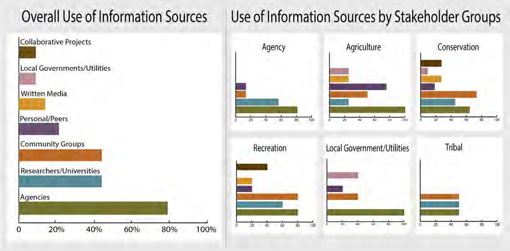
Figure 8-4. The left graph shows how often different sources of information were mentioned in interviews. The six right-side graphs show how the use of these sources differed among stakeholder groups. When the information source was mentioned at least once in all interviews, the value is 100%.

Agencies were the most utilized information source by far, referenced in 80% of all interviews. Community Groups and Researchers/Universities were the next most common, with both sources utilized by almost half of the participants. However, Community Groups were a much more common information source than Researchers/Universities for all stakeholder groups except Agency staff. The apparent popularity of Researchers/Universities as a source likely reflects the relatively large number of Agency interviewees in our sample.

We also found that many participants were likely to use data that their own stakeholder group produced. Conservation participants used a significant amount of Community Group information, probably because most interviewees were members of environmental nonprofit organizations. Similarly, Local Government/Utility participants were more likely to use data from Utility entities and city planning departments. Agricultural producers often mentioned that they use Personal/ Peer observations, meaning that the information ultimately came from other farmers and ranchers. Interestingly, that was not the case for Recreation participants, who seldom mentioned Personal/Peer observations.

Figure 8-5 shows the types of environmental and climate change information distributed by various sources. Agencies were the primary source for nearly all types of information. Water information came from all five major sources (Agency, Personal/Peer observations, Community Groups, Researchers/Universities, and Local Government/Utility information). vegetation and habitat data had two sources (Agencies and Researchers/Universities), while species and weather information came in part from a third source (Personal/Peer observations).

Figure 8-6 shows how often these types of information were referenced by different GYA stakeholder groups. Water information was most utilized by all groups to a large degree. The next most popular type was weather information, but it was consulted less often than water information, although a crossover likely exists between these two categories given the impact of weather on the water balance (see Chapter 7). Most participants used just water and weather information, although some Local Government/Utility participants used vegetation and habitat data. Agency participants used many types of information. The limited number of Tribal participants prevented us from quantifying the types of information they used.

Figure 8-5. Each chart shows the sources that stakeholders used to access information about a given topic.

Figure 8-6. The left chart shows the relative usage of different types of information. The right five charts break the information types down by stakeholder group use. We lacked sufficient data from Tribal members to quantify relative data usage for this group.

INFORMATION NEEdEd

We asked participants: What information would you like to have about changes in seasonal patterns and environmental uncertainty, and what format or medium is most useful to you for sharing this information?

Once we understood the information that stakeholders currently use, we then asked what kinds of information they would like to have. Some participants simply wanted more or better versions of the data already available to them, while others had needs that were not currently being met. Thus, the desired information either was not easily accessible or did not exist. We also heard about ways that information could be presented more effectively or made more relevant, as well as the formats and mediums that are most effective.

At least half of participants in all groups mentioned a need for more information on water, even though it is already widely used. Many participants specifically mentioned the need for higher resolution data to enable better understanding of the changes underway in their watershed. For example, an Agency participant in the Upper Yellowstone watershed explained, “We don’t understand how precipitation is going to change in space and time. We could really use more realtime streamflow monitoring on small and medium sized streams.”

More weather information, including current data and future projections, was also a common request for all stakeholder groups. In fact, climate and weather information was mentioned as a need as often as the need for water information by Agriculture and Conservation participants. Additional information on fish and wildlife, and vegetation and habitat was requested by Recreation and Agency participants, who recognized its relevance for outdoor tourism and resource management.

More weather information, including current data and future projections, was [a] common request for all stakeholder groups.

Regarding preferred formats: Conservation, Recreation, Local Government/Utility, and Agency participants all agreed that maps and other visuals are key. Participants also agreed that these materials should be accessible online, although some Agriculture participants asked that important materials also be available in print, so that less technologically savvy individuals could access them.

Messengers Matter: How to Keep Data Accessible and Relevant

Many of the participants in our interviews had important insights on how climate and environmental information could be made more available or relevant. For example, many asked for what an agency member from the Snake Headwaters watershed described as, “an open source, user friendly platform” to serve as a comprehensive information hub. The platform could be organized by the state or watershed to cover a wide range of climate topics, including drought and fisheries health, as a centralized and regularly updated source of environmental data. Many interviewees felt that compiling information in this way would greatly boost accessibility to these topics.

Beyond data accessibility, it was equally important that information be digestible for a range of audiences. It was suggested that climate and environmental information be framed and conveyed in a way that would be useful and usable for different communities. To do so, some participants asked that climate change information be presented in the context of present conditions, rather than in the past or even the future. A Conservation participant in the Missouri Headwaters watershed stated, “Everything to do with projections is a sore subject for me. Nobody cares about what’s happening in 2080. That’s just not compelling to anybody... because there is so much uncertainty about projections.”

Others cautioned against “speaking to the choir” and emphasized the importance of using clear terminology and trusted messengers. Information on climate and environmental change should be conveyed by groups or individuals that are locally known and respected, such as conservation districts.

I’m not in the young [rancher] group, but the online ranching magazine sources—Wyoming Livestock Roundup, Drover’s Journal—ranchers trust those. Agricultural media they’ll trust.”

— agriCUlTUral prodUCer, Upper green waTershed

Ultimately, information is only valuable if it is accessible. The ongoing effort to educate Greater Yellowstone’s communities on climate change will require both modern platforms and trusted messengers to bridge the gap between researchers and stakeholders. Taken together, feedback from our interviewees provides valuable insights into how to do this.

Long-term Monitoring for the Future of the Greater Yellowstone Area

David M. Diamond, Greater Yellowstone Coordinating Committee; Kristen L. Legg, National Park Service; David P. Thoma, National Park Service; Andrew M. Ray, National Park Service

The plants, animals, streams, glaciers, air quality, and climate of the GYA are monitored to assess the health and changing conditions of the ecosystem. This information helps land managers, communities, and landowners decide when and where to take action to minimize undesirable change. The following are examples of how long-term monitoring is being applied across the GYA:

о Clean Air Act.—The Clean Air Act Amendments of 1977 mandated regular monitoring of air quality in all national parks and wilderness areas. In addition to the dangers for human health, air pollution and deposition of pollutants in water and soils can remove soil nutrients, injure vegetation, and acidify and over fertilize lakes and streams. For over 20 yr, Yellowstone and Grand Teton national parks have operated air quality monitoring stations that track the deposition of sulfur, nitrogen, ozone, and particulate matter in the region (NPSa undated).

о Greater Yellowstone Network.—For almost two decades, the National Park Service-Greater Yellowstone Network (NPSb undated) has monitored vital signs of ecosystem health, including changes in climate, water quantity and quality, amphibians, wetlands, and whitebark pine (Ray 2019). This network, one of 32 managed by the National Park Service, provides park managers, researchers, and the public with updated scientific information on natural resources in the federal lands of the GYA. Through collaboration with federal agencies, universities, non-governmental organizations, and the public, vital signs monitoring will continue to be an important component of science-based decisionmaking to maintain functioning ecosystems into the future.

The Greater Yellowstone Network utilizes data collected at NOAA weather stations and USGS streamgages located throughout the region. Some stations and gages that have been in place since the early 1900s offer an opportunity to understand historical changes in climate and river flows (see Chapter 3). The Yellowstone and Grand Teton dashboards on the Climate Analyzer (undated) offer a way to explore weather and streamflow data.

surveying for amphibians. Photo credit: National Park Service.

о National Ecological Observatory Network (NEON).—In addition to the Greater Yellowstone Network, efforts are underway in the GYA to monitor the overall health of the ecosystem. In 2018, NEON—a national network of ecological observatories supported by the National Science Foundation— established a field site in northern Yellowstone National Park, outfitted with atmospheric, soil, and aquatic sensors to monitor climate-driven changes (NEON undated). The Yellowstone site is one of the 81 sites across the country that together aim to provide continuous long-term and continental-scale observations of ecological change.

о RiverNET.—Other monitoring efforts in the GYA include RiverNET, a program launched by the Yellowstone Ecological Research Center in 2018 (YERC undated). The goal of RiverNET is to gather water quality and flow information along a stretch of the Yellowstone River north of Yellowstone National Park. Data from this effort will provide the information needed to detect shifts in stream conditions from changes in climate and land use. The design of RiverNET is intended to be transferable to other watersheds in the GYA.

о Greater Yellowstone Coordinating Committee (GYCC).—Researchers are studying glaciers, snow, and icefields of the GYA to understand how they are changing (see boxes, Chapters 2 and 3). The GYCC (GYCC undated) has sponsored efforts by the US Forest Service and National Park Service to create a long-term monitoring program of glaciers in the Teton, Wind River, and Beartooth ranges (USFS undated). The program in Grand Teton National Park visually captures the transformation of the glaciers using repeat photography and other measurements of ice volume and flow (NPSc undated). Artifacts emerging from melting snow and icefields in the GYA are providing a wealth of biological and cultural information dating back as far as 10,000 yr (see box on snow and icefields, Chapter 2).

Findings from these long-term monitoring programs help us to understand when, where, and why a species or ecological processes becomes vulnerable. For example, while drought can occur any time, climate projections suggest that late-summer drought will increase in the coming decades (see Chapter 7). Understanding which species are most susceptible and where drought is likely to be most intense helps managers anticipate where action might be needed. For example, a) amphibian species, such as the boreal chorus frog, are more susceptible to drought than longer-lived species that can avoid breeding during the driest years; and b) the extent of wetlands in the southwestern corner of Yellowstone National Park are more susceptible to drought than those in the seemingly drier northern part.

Another example of how long-term monitoring informs ecosystem health is tracking whitebark pine in the GYA. Many of the large, cone-producing whitebark pines have been killed over the past decade by mountain pine beetle. The recent beetle epidemic resulted from warm winter temperatures that caused mountain pine beetle populations to explode and move to higher elevations into whitebark pine forests (see box on wildfire, Chapter 5). At the same time, non-native blister rust fungus is also killing whitebark pines, and its spread is favored by high humidity. Knowing how temperature and humidity influence the diseases and pests that kill pine trees helps managers decide where protection and planting of new seedlings are likely to succeed. Monitoring forest health, in light of future climate projections, may help give one of the GYA’s most majestic conifers a better chance at survival in the decades ahead.

LEAdERS ANd CuRRENT WORk

We asked participants: Who is leading work in your community on resilience or adaptation projects related to environmental uncertainty? Where is it being done? What are they doing?

We were interested in participants’ knowledge of groups working to address climate change—be it through mitigation, resilience, or adaptation—and the specific projects those groups were leading. Though there were exceptions, participants were mostly aware of leaders in their stakeholder group.

Participants’ knowledge of projects was also tied to their expertise, which, for many, was water. For example, Agency participants mentioned projects that focused on water supply, communities, and aquatic species projects. Most Agency participants worked as habitat or species-specific biologists, which may explain why water and habitat-related projects were mentioned often. Several monitoring efforts are also already underway on federal lands, which Agency interviewees were particularly aware of given their involvement in monitoring work (see box).

Other projects mentioned by participants varied widely, and included fuel reduction, cheatgrass management, beaver translocations, Zeedyk structure implementations, and native fish restoration. Note that many of these projects serve more than one objective. For example, a habitat restoration project might also stabilize a bank from erosion and provide more shade, thereby reducing temperature and improving water quality for fish. This may help explain the variety of responses we received, since any given project can be described multiple ways depending on one’s own knowledge and priorities.

Current work by stakeholder group

Agriculture participants most often mentioned projects related to water supply, water quality, and vegetation, as well as projects related to fish and wildlife. Their list of projects further emphasized the importance of adaptation efforts in agriculture; for example, work on soil microbes to improve soil health was mentioned by several participants. A producer in the Upper Snake watershed brought up “alternative crops,” suggesting “fall wheat instead of spring wheat. The fall grain… it’s coming up as soon as the snow melts. It requires roughly one less irrigation [cycle] during July, and that saves some water.” The importance of adaptive irrigation was also mentioned even by many non-agriculture participants, including a Recreation participant in the Upper Yellowstone watershed who noted that “most [agricultural producers] are used to the wildly fluctuating weather. Many established folks have stock ponds and water storage and are used to rolling with the punches.”

Local Government/Utility participants spoke mostly about projects related to their work on water supply and quality, and community projects. One participant in the Missouri Headwaters watershed talked about efforts to upgrade hydropower facilities, “increasing the flexibility of the power plants to efficiently generate through a wider range of flow conditions.” An Agency participant in the Upper Snake watershed spoke about Local Government/Utility work, citing the city of Chubbuck ID and how it invested in wastewater infrastructure by installing “water lines and wastewater lines into easements that extend far outside the city in preparation for growth.”

Changes Rippling Through Our Waters and Lives

Christine N. Martin (Little Big Horn College); John Doyle (Crow Tribal member, Little Big Horn College); JoRee La France (Crow Tribal member, University of Arizona); Myra J. Lefthand (Crow Tribal member, Little Big Horn College); Sara L. Young (Crow Tribal member, Little Big Horn College); Emery Three Irons (Crow Tribal member, Little Big Horn College); Margaret Eggers (Montana State University)

The Crow Reservation is located in south central Montana, in the heart of our traditional homelands. As we live in a wide-open landscape and are tied to a different time than the fast pace of western life, our understanding of nature and observations of the seasons comes from the eye instead of a calendar or watch.

Climate change is already impacting our lands, our waters, our health and well-being. To better understand these impacts, we interviewed 26 Crow Elders about their perceptions of changes in local weather patterns and ecosystems throughout their lifetime, and how they are being affected. We conducted a thematic analysis of the interviews.

Interviewees’ observations paralleled and elaborated on instrumental climate data: We are experiencing far less snowfall and milder winters, increased spring flooding, hotter summers, and more severe wildfire seasons. Additionally, many Elders commented on extreme, unusual, and unpredictable weather events, compared to earlier times when the seasons were consistent year after year.

Bill Lincoln picking chokecherries on the Crow Reservation (photo courtesy of John Doyle)

Interviews notably identified declines in wild foods, which have not been recorded by scientists; wild game, fish, berries, and medicinal plants are being detrimentally affected in diverse ways. Our homes and infrastructure have been hit time after time by high floods; we have few resources to repair the damage, so this is taking a toll on families, including on our health and well-being.

In addition to ecosystem resource losses and changes, we are devastated by the loss of coal jobs and coal tax revenue. More than 1200 coal mining and tax-funded jobs have been lost in the past couple years, in a community of about 8000 people. Without that income and lacking any other tax structure, we cannot adequately fund our government nor maintain our infrastructure.

Through the research we have been conducting on climate change and with our Tribal Elders, we are able to better understand what has been happening and anticipate what is to come. Although we are enduring unprecedented environmental change and extreme economic conditions, we are looking for solutions we can implement ourselves.

For more information, see Martin et al. (2020).

Conservation participants were most aware of ongoing projects that had a community emphasis. Participants mentioned multi-stakeholder initiatives, including the Upper Yellowstone watershed Group. This group is one example of many working to address climate change by developing a drought management plan for different stakeholders if faced with drought conditions in the future.

Recreation participants were also more likely than others to know about work being done within their group. For example, one participant in the Upper Yellowstone watershed spoke about his company’s efforts to connect their clients to the reality of climate change by sending thank you emails to clients that contained conservation information and links to relevant organizations. The company also looked for fishing and hunting guides with training in programs that include a conservation component. The participant was also familiar with community groups, like environmental organizations, leading projects related to water availability and aquatic species. This familiarity may reflect the fact that many non-governmental organizations push for community and business involvement.

Across all stakeholder groups, needs for policy and water-related projects (especially to address water supply issues) were mentioned more than any other category.

Results considered by watershed

By comparing projects across watersheds, it was possible to see where and what climate-related work is being done. The Missouri Headwaters and Upper Yellowstone watersheds clearly stand out as places where adaptation efforts are underway by Agency, Recreation, Agriculture, Local Government/Utility, and Community group stakeholders, although no interviewee was fully aware of all efforts in their watershed. Discussions and insights provided by Tribal members indicate their concerns and efforts to confront climate change, including building resiliency and sharing information, as well as the limited knowledge that others have of these efforts (see boxes).

pROjECT NEEdS

We asked participants: If there are no resilience or adaptation projects in your community, do you perceive a need for such efforts? If so, please say more about what would best serve you and your community.

We were interested in learning about gaps in the work currently being done, allowing stakeholders to describe their group’s unmet needs. By comparing the responses by group and watershed, we can better understand what projects are most needed within groups and across the GYA. As with the previous question, responses about project needs varied widely.

Across all stakeholder groups, needs for policy and water-related projects (especially to address water supply issues) were mentioned more than any other category. Other prominent needs related to more monitoring and data collection, funding and human resources, efforts in habitat and species conservation, and wildfire mitigation projects, in that order.

Agency participants cited the need for projects to improve habitat, undertake more extensive monitoring, and protect water supplies, all of which require additional resources and funding. One Agency participant in the Upper Snake watershed described their unique needs as resource managers, explaining, “One of the issues that we still struggle with is to have common information utilized by multiple agencies… We all have access to some of the same information, but some agencies have a different mission than others and utilize the information differently. It’d be nice to have a consortium of these interest groups come together to describe how they use data and try to reach synergy in how the data is used to make management decisions, because we’re concerned that sometimes decisions are made that are in conflict.”

Multiple Agency participants focused on improving their interactions with agricultural producers. For example, some Agency participants emphasized that there was a huge gap in understanding the goals of their staff versus those of agricultural producers. One Agency participant in the Big Horn watershed wanted to “facilitate changes so agriculture producers can stay ahead of the game [of climate/water changes], rather than respond to the problem when it comes... the changes really need to be made in small producers, but the small producers need a return on investment right away, which can be difficult to provide.” Another Agency member from the Big Horn watershed highlighted that “the elephant in the room is the diversions for agriculture use. Many of the streams and rivers in Wyoming are over allocated. There needs to be gages on all the head gates and better enforcement on that… We need them to acknowledge that they care and they are part of the problem. We’re all in this together.”

“We’re all in this together.”

— agenCY MeMber, big horn waTershed

Agriculture participants most frequently mentioned the need for projects to monitor water supply or water quality, as well as for more available project funding. These needs often centered on irrigation. As one Agricultural producer in the Upper Green watershed stated, “I think we’re going to have less water to irrigate, and as irrigators we’re going to need other methods.” Interestingly, the producer went on to point out potential opportunities pending available water, saying, “I think what you’re also going to see in climate change, which is going to be a benefit to this valley and a benefit to… high [elevation] areas, is we’re going to have longer growing seasons, we’re going to be able to grow more… there’s going to be more agricultural opportunities in cultivated ground if there’s any water left.” Another Agricultural participant in the Upper Yellowstone watershed related future water supply and quality to issues of housing development on the rural landscape. That individual explained that “open space is going to be a crucial issue to water going forward. Any time you’ve put a house on it you change the water. Housing development has more runoff from nitrates than a ranch does because they’re trying to keep their lawns green.”

Upper Snake River Tribes Foundation Climate Change Vulnerability Assessment

S. Petersen (Adaptation International [AI]); J. Bell (AI); S. Hauser (Upper Snake River Tribes Foundation); H. Morgan (University of Washington Climate Impacts Group [UWGIG]); M. Krosby (UWCIG); D. Rupp (Oregon Climate Change Research Institute [OCCRI]); D. Sharp (OCCRI); K. Dello (OCCRI); and L. Whitley Binder (UWCIG)

In 2017, Upper Snake River Tribes (USRT) Foundation Climate Change vulnerability Assessment (Petersen et al. 2017) was released as a collaborative project of the USRT Foundation and its member Tribes (ShoshoneBannock Tribes, Shoshone-Paiute Tribes, the Fort McDermitt Paiute-Shoshone Tribes, Burns Paiute Tribes). The report considers the species, habitats, and resources that are important and valuable to USRT member Tribes. Climate change impacts on these resources have the potential to affect Tribal members’ culture, spirituality, and lifeways. Combining the best available climate projections for the region with traditional knowledge, Tribal priorities, and local observations was central to the success of the assessment effort.

The report includes: 1) a summary of downscaled future climate projects for the eastern Snake River Plain; 2) a detailed description of the vulnerability assessment progress and outcomes; 3) discussion of the Tribes’ adaptation planning process; and 4) a listing of the adaptation actions developed for the plant and animal species assessed. The goal has been to lay a foundation for building resilience among the USRT member Tribes and enhancing the resilience of natural resources that are an integral part of the culture.

A Climate Change Core Team of Tribal staff worked collectively with outside consultants to identify those aspects of climate change that were of greatest concern and determine appropriate adaptation actions for critical plant and animal species and their habitats.

The Core Team identified 35 plant and animal species, seven resource issues, and four habitats of concern for inclusion in the assessment. Thirty-four species were assessed quantitatively using NatureServe’ Climate vulnerability Index (CCvI), which evaluates vulnerability in light of projected changes in air temperature, moisture availability, species range data, and species-specific life history characteristics. Project consultants and the Core Team worked collaboratively to vet preliminary CCvI results and integrate local and traditional knowledge (as appropriate) in assigning final species’ vulnerability rankings.

The final phase of the vulnerability assessment project focused on developing strategies and actions to increase the resilience of the habitats where the assessed species live. Due to the interconnected nature of the ecosystems and habitats on which these species depend, adaptation planning focused on developing strategies and actions that would strengthen the climate resilience of habitats, thereby supporting the needs of the individual species.

The report concludes:

Changing climate conditions have already altered and will continue to affect the natural resources, landscapes, and people of the Upper Snake River watershed. By taking the initiative to explicitly identify Shared Concerns and assess their climate change vulnerability, the USRT’s four member Tribes have begun the process of climate change adaptation.

Conservation participants described the need for more monitoring and data collection, changes in policy, and additional projects that address water supply, fish and wildlife, and habitat. A participant in the Upper Yellowstone watershed described the most pressing needs, as follows:

“[M]ore information and data is a big need… the awareness is already there, but we need more information and tools in the toolbox.”

— ConservaTion sTakeholder, Upper YellowsTone waTershed

Local Government/Utility participants cited the need for projects focused on water supply, policy change, and new monitoring and data. One participant from the Missouri Headwaters watershed spoke about a new way to monitor and manage water usage, and the need for other communities to adopt it. The system monitors “residential and commercial use by the hour,” ultimately helping quickly identify problems such as unusual spikes in usage. Other Local Government/Utility participants focused on better water management in drought years and better planning for water shortages.

Recreation participants cited the need for new policy, new habitat and conservation projects, and new efforts to monitor water supply. Habitat projects to improve the health of tributaries for fish spawning or to maintain cool water temperatures were of particular interest. Like Agency participants, Recreation interviewees also mentioned the need to work with Agricultural producers to ensure that water is used more effectively. A Recreation participant in the Upper Snake Headwaters watershed explained, “Some of that [water use] may require changes in water law because many senior water rights holders are afraid they’ll lose their water rights if they don’t use them every year… this change is necessary to reflect the fact that water is now recognized as important not just for irrigation, but also for fish, recreation economies, etc.”

Our Tribal participants spoke about policy and monitoring needs:

“Given that the bulk of stewardship [for the Tribes] happens locally, it would serve our community to have a greater sense of guiding stewardship discussions and planning in the Greater Yellowstone Ecosystem. We are the original inhabitants of the area and our traditional ecological knowledge should hold a significant place in contemporary management discussions. Often our priorities are in line with the top-order goals of preserving the Greater Yellowstone Ecosystem, but we seem to have a disconnect with lower order objectives and strategies for achieving those goals. One example might be forest management, where the risk of a stand replacing fire is high the Forest Service might prefer a logging operation, where the Tribes may prefer thinning and re-introducing fire back into that landscape to mitigate the risks.”

— Tribal MeMber, Upper snake waTershed

By looking at project needs across watersheds, we can start to visualize these types of projects on a spatial scale. For example, needs related to water and policy were mentioned in all six of the watersheds. We also identified needs for monitoring and data collection, and for additional funding and resources. Highest priorities were related to protecting water supplies, fish, and wildlife.

pOLICY

We asked participants: What policy efforts are underway related to changes in environmental factors, seasonal patterns, and climate? How can we build on them?

Our intent in asking participants about climate change policies was to gauge their awareness of and opinions on this topic. Notably, stakeholders’ views and understanding of policies do not necessarily reflect the regulatory landscape present in the GYA, nor the past, current, or potential future policies of federal land management agencies, state agencies, local governments, or Tribal governments. Our findings presented here in no way should be considered recommendations by entities that collaborated on this Assessment.

Many participants were unaware of current policies that address climate change and water. An Agency participant in the Upper Green watershed said, “I don’t know of regional policy… or true initiatives at state or county level.” Participants also brought up how it is hard to stay informed about current policy and the impact that it has on a state level.

“In Wyoming in particular, the state delegation has been slow to react to the issue of climate change and thus need more public input, which means the public must first have the information to convey the issues in an educated manner...information regarding policy is not always easy to find or research.”

— reCreaTion inTerviewee, big horn waTershed

Some participants talked about recent rollbacks of climate change and water policies. A Tribal member in the Upper Snake watershed said, “During the past four years, the wide shift in [federal] administration policy has taken us years back in terms of managing to alleviate the risks

Left: Arapaho Language Symposium. Photo courtesy of Crystal C’Bearing.

Right: Montana public lands rally. Photo courtesy of Scott Bischke.

of climate impacts.” Other interviewees expressed frustration about the policy makers’ lack of transparency in setting climate change policies and their denial about the topic of climate change. A Conservation participant in the Big Horn watershed lamented, “My overwhelming sense is all policy efforts from the national to the state level are related to denying changes in environmental factors and we are in a crisis. We do not hear from agencies about what they are doing because they learned not to raise their heads even though there may be some of that occurring quietly.”

When aware of existing policy efforts, participants mostly spoke about policies that their organization, agency, and/or company were working on, developing, or advocating for. Most of these policies are at an agency level. For example, Agency participants spoke about their work to address climate change in state-level habitat plans, with one member in the Big Horn watershed emphasizing the importance of project prioritization to allocate funding and personnel effectively. Other agency participants mentioned that some agencies have groups specifically assigned to address climate adaptation, including the Greater Yellowstone Coordinating Committee1, which has a subcommittee on Climate Change Adaptation, and the Custer Gallatin National Forest’s Climate Adaptation Group.

At a federal level, some participants noted the need to elect legislators who are concerned about climate change so that traction could be gained for large-scale policy initiatives. A Conservation participant in the Missouri Headwaters watershed put this idea in perspective, saying that “telling Montanans that turning off your lights is going to deal with the issue is setting false expectations and is not honest.”

“The single most important thing we can do in 2020 is [to get our legislators to] adopt a climate platform.”

— ConservaTion parTiCipanT, MissoUri headwaTers waTershed

Calls from stakeholders for future policies related to climate change often highlighted the importance of cooperation. One Conservation participant from the Upper Snake watershed alluded to the need for more “regional coordination,” and a Recreation interviewee in the Upper Yellowstone watershed expressed the need for all watershed members to work more closely together to address water needs in a changing environment. That individual stated, “The key is changes to water law to reflect that water is not just a resource to be used in the traditional sense for irrigating, and that we all have a stake in the river and its health and that we aren’t fighting each other.”

Participants in every watershed of the GYA spoke about policy needs. However, their answers varied so widely that it was difficult to extract any common themes. More specific follow-up questions need to be asked to better understand current efforts to develop policy from a geographical perspective.

1 The Greater Yellowstone Coordinating Committee (GYCC) is made up of 12 federal land managers in the GYA, including representation from the Forest Service, Bureau of Land Management, National Park Service, and Fish and Wildlife Service as well as the directors of Idaho, Montana, and Wyoming’s state fish and game agencies. The GYCC allows the federal land managers in the Greater Yellowstone Ecosystem to pursue opportunities for voluntary cooperation and coordination at the landscape scale.

Climate and Reciprocity for the Eastern Shoshone Tribe

Wes Martel (Be-ku’-naw), Eastern Shoshone

On August 11, 2020, a tornado touched down 6 miles northwest of Riverton, Wyoming. In the Shoshone oral tradition of passing down stories from elders to youth for millennia, we have no history of tornados in our ancestral homelands. Our climate is changing.

Serving on the Eastern Shoshone Business Council for 20 yr beginning in 1979 was an honor and privilege of a lifetime. Being in this position not only gave me the wonderful opportunity of getting to know the families and relatives of the Shoshone Tribe, it also empowered me to understand how governance is exercised by Tribes without a Constitution. It has been my responsibility to breathe life into our treaties and rid ourselves from the devastating impacts of colonization. This is one approach to take care of our people, our land, waters, and our climate.

In the Chambers of the Joint Business Council of the Shoshone and Arapaho Tribes hang two large portraits. One of Chief Washakie of the Eastern Shoshone and one of Sharp Nose of the Northern Arapaho. Sometimes when I was alone in the Chambers, I would look up at these two men and they would seem to be looking at me asking, “What are you doing to help the people?” I tried to imagine the tremendous pressure and heartache they must have endured when the way of life they knew was being threatened. When Chief Washakie signed the Eastern Shoshone Treaty of 1863, whereby the United States recognized Tribal rights to 44,000,000 acres (17,000,000 hectares) of land in Wyoming, Idaho, Utah, and Colorado, there must have been some sense of relief that a way of life would be protected and allowed to flourish in traditional homelands and hunting and gathering grounds. Promises made to protect and support the Shoshone people in this 1863 Treaty were ignored five years later in the Treaty of 1868, which reduced the Shoshone Reservation to 2,500,000 acres (1,000,000 hectares).

Even after this severe transgression, the Shoshone people never lost their connection to this land that sustained them since time immemorial. The Greater Yellowstone Area was their garden, pharmacy, church, hospital, grocery store, and park, amongst many other uses. This abundance of life-sustaining gifts was respected and revered with the “you take care of us, we take care of you” belief that is the cornerstone of Indigenous values and beliefs. This reciprocity is a way of life that has empowered us to weather the many storms of colonization and inequity.

The monetary value attached to that which is provided by Mother Earth has led to destruction of resources and caused irreparable harm to lands, waterways, and air. This natural imbalance can be seen through fires, mudslides, tornadoes, hurricanes, floods, and other violent weather events that are ever more frequent and more destructive. Indigenous people understand the calamity will continue until the reciprocity of “you take care of us, we take care of you” is strengthened and restored. This is more than governance. It is spirituality in its most open and literal sense. The Indigenous connect to all above ground and all below ground through a spiritual inter-connectedness that transcends physicality.

I have witnessed humble Indigenous men and women perform healing and spiritual connections that most modernday religious leaders could only dream of. The reason for this gift is a full recognition of the spirit within all animate and inanimate beings. The wind, the lightning, the tornado, the fierce storms that are becoming more common have a spirit. Indigenous people used to have many elders who understood how to communicate with this spiritual realm, but numbers are dwindling. We are losing this critical connection. Can Indigenous people help reverse this? Maybe. We were all Indigenous at one time and understood the need to be thankful.

There remains a strong Indigenous connection to the GYA. For the most part, those of us fortunate enough to live within the GYA are incredibly thankful to be from this part of the world. GYA has been “taking care of us.” We must renew our efforts to the GYA to “take care of you.” The Indigenous connection of the GYA spans the Native Tribes in the United States and Native Bands in Canada. These entities exercise governance in the forms of policies, codes, standards, regulations, guidelines, and other management and enforcement actions, and these values and beliefs are recognized by the United States Government through environmental and antiquities laws.

Tribal and Band governments have difficulty in assembling the administrative and technical capabilities to address grassroots concerns for protecting rivers and traditional human uses. The reach of Indigenous governance, however, should begin by recognizing reciprocity as a catalyst to return to our Tribal heritage and revive reciprocity as the dominant force in respecting the GYA. For anyone that has ever experienced the GYA, it never rubs off. It remains in our hearts and our minds and our spirits because of its power and spirit. We feel it. We live it. We breathe it. We must correct the imbalance for the benefit of our climate.

SuMMARY

In the face of climate change, the fate of communities and environments depends on people. For the GYA, climate change mitigation and adaptation will ultimately be defined by the views and actions of its people.

Our interviews show that those stakeholders, even with greatly varying backgrounds, feel common concerns regarding climate change. For this reason, continued stakeholder engagement, to gauge their needs and learn from their perspectives, presents an important opportunity to improve GYA science and adaptive management outcomes. To this end, no substitute exists for real relationships, conversations, and curiosity.

We gleaned many important takeaways from the 44 interviews summarized here. We learned that water is most people’s primary focus, both in terms of their current efforts and observations, as well as the work already underway. Specific impacts included drought, spring runoff, and declining native fisheries. We also found that, while water supply is often the main concern, many community members also recognize that addressing water issues will benefit other aspects of the environment, as well.

Overall, GYA communities are clearly aware of the looming threats from climate change. The findings here can help us better inform and prepare to face those threats.

LITERATuRE CITEd

Climate Analyzer. [undated]. The climate analyzer [website]. Available online http://www.climateanalyzer. org. Accessed 13 Jan 2021.

[GYCC] Greater Yellowstone Coordinating Committee. [undated]. About [webpage]. Available online https:// www.fedgycc.org/about. Accessed 8 Mar 2021.

Martin C, Doyle J, LaFrance J, Lefthand MJ, Young SL, Three Irons E, Eggers M. 2020. Change rippling through our waters and culture. Journal of Contemporary Water Research and Education 169:61-78. https://doi. org/10.1111/j.1936-704x.2020.03332.x.

[NEON] National Ecological Observation Network [undated]. About field sites and domains [webpage]. Available online https://www.neonscience.org/field-sites/about-field-sites. Accessed 8 Mar 2021.

[NPSa] National Park Service [undated]. Grand Teton National Park air quality [webpage]. Available online https://www.nps.gov/grte/learn/nature/airquality.htm. Accessed 8 Mar 2021.

[NPSb] National Park Service [undated]. Greater Yellowstone Inventory and Monitoring Network [webpage]. Available online https://www.nps.gov/im/gryn/index.htm. Accessed 8 Mar 2021.

[NPSc] National Park Service. [undated]. Glacier monitoring [webpage]. Available online https://www.nps. gov/grte/learn/nature/glaciermonitoring.htm. Accessed 8 Mar 2021.

Petersen S, Bell J, Hauser S, Morgan H, Krosby M, Rudd D, Sharp D, Dello K, Whitley Binder L. 2017. Upper Snake River climate change vulnerability assessment. 131 p. Boise ID: Upper Snake River Tribes Foundation]. Available online http://www.uppersnakerivertribes.org/climate/. Accessed 8 Mar 2021.

Ray, AM (ed). 2019. vital signs: monitoring Yellowstone’s ecosystem health [multiple articles]. Yellowstone Science 27 (1). Available online https://www.nps.gov/articles/upload/Yellowstone-Science-27-1-vitalSigns_revised.pdf. 97 p.

[USFS] US Forest Service. [undated]. Bridger Wilderness glacier monitoring [webpage]. Available online https://usfs.maps.arcgis.com/apps/MapSeries/index.html?appid=a5e0a5a1d08549d194415f10aefb3c37. Accessed 8 Mar 2021.

[YERC] Yellowstone Ecological Research Center. [undated]. RiverNET: community science in action [webpage]. Available online https://www.yellowstoneresearch.org/rivernet. Accessed 8 Mar 2021.

University of Wyoming biologist documenting a Yellowstone Cutthroat trout

Photo courtesy of Emily Reed

Hayfield, Madison Valley, Montana

Photo courtesy of Rick and Susie Graetz

9. CONCLUDING REMARKS

Cathy Whitlock, Steven Hostetler, Bryan Shuman, David Liefert, Charles Wolf Drimal, and Scott Bischke

This Assessment of climate and water in the Greater Yellowstone Area (GYA) shows that climate trends and variability that have been part of the GYA’s past will continue to be part of its future. Past climate trends are evident from a variety of geological and paleontological data sets in the region as described in Chapter 2. During the last glaciation (22,000-13,000 yr ago), the GYA was 5-7°F (3-4°C) colder than the pre-industrial period (1850-1900). The glacial period was terminated by a warming trend that led to rapid glacial recession and forest colonization. By the early Holocene (11,500-7000 yr ago), the climate was up to 3.8°F (2°C) warmer than the pre-industrial period. Climate variability in the GYA has also occurred in the past. For example, there have been dramatic fluctuations between wet and dry periods in the last 1000 yr. The last 20 yr (2001-2020) stands out as the warmest period of at least the last 20,000 yr in the GYA, and probably longer. Atmospheric greenhouse gases (GHGs) have not been at the current level for the last 3.3 million years.

Past climate changes were caused by natural climate drivers (e.g., Milankovitch cycles, changes in atmospheric composition, volcanic activity, solar output, and atmosphere-ocean circulation). In addition to the consequences of natural drivers, the climate of recent decades has been warming as a result of human-caused emissions and attendant increases in GHGs. Based on weather station data, the GYA has warmed on average by 2.3°F (1.3°C) since 1950 (see Chapter 3). This warming has resulted in a growing season that now is 2 weeks longer than it was in the 1950s, and below 8000 ft annual snowfall has declined by 25% (nearly 24 inches), including by 96% in September. The rapid warming that marks the end of winter now occurs in February to March, instead of March to April as it did in 1950. Melting of the snowpack is also occurring earlier in the year, and peak annual stream runoff now occurs on average 8 days earlier than it did in 1950.

Based on weather station data, the GYA has warmed on average by 2.3°F (1.3°C) since 1950 (see Chapter 3). This warming has resulted in a growing season that now is 2 weeks longer than it was in the 1950s, and below 8000 ft annual snowfall has declined by 25% (nearly 24 inches), including by 96% in September. The rapid warming that marks the end of winter now occurs in February to March, instead of March to April as it did in 1950. Melting of the snowpack is also occurring earlier in the year, and peak annual stream runoff now occurs on average 8 days earlier than it did in 1950.

The magnitude and rate of projected future warming are determined by the amount of GHG emissions into the atmosphere. We based the Assessment on two of the internationally used scenarios of future GHG emissions, Representative Concentration Pathways 4.5 and 8.5 (RCP4.5 and RCP8.5). RCP4.5 is an intermediate scenario in which the rate of emissions is curtailed and stabilizes by 2080; RCP8.5 is an upper bound scenario in which emissions continue to increase through the end of century (see Chapter 4). These two pathways differ in their related projections of GYA’s climate future. By the end of century, temperatures in the GYA could range from 5-6°F (2.8-3.3°C) warmer than our 1986-2005 base period under RCP4.5, to as much as 10-11°F (5.66.1°C) under RCP8.5 (Figure 9-1; see Chapter 5). Over the next 20 yr (2021-2040), the projected warming of 2.5-2.9°F (1.4-1.6°C) under RCP4.5 and RCP8.5, respectively, is about the same as occurred between 1950 and 2005. After 2040, the projected rate of warming until the end of century will be about twice that of the 1950-2005 period under RCP4.5 and nearly five times greater under RCP8.5. In both cases, temperature increases will bring warmer days and nights, warmer winters, and hotter summers in the coming decades. These warmer conditions will affect water supplies, natural and managed ecosystems, economies, and human and community wellbeing in the GYA.

[T]emperature increases will bring warmer days and nights, warmer winters, and hotter summers in the coming decades. These warmer conditions will affect water supplies, natural and managed ecosystems, economies, and human and community well-being in the GYA.

Figure 9-1. Historical changes in temperature (black line) are described in Chapter 2, and future projections for Representative Concentration Pathway 4.5 (RCP4.5, blue line) and RCP8.5 (red line) are described in Chapter 5. The colored lines for the RCP data are the median of 20 global climate models (GCMs) in the MACAv2-METDATA downscaled data set and the respective shaded bands around the lines are the 10th (lower) and 90th (upper) percentiles of the models.

Little Bighorn River swimming hole at Crow Agency, Montana

Photo courtesy of John Doyle

Annual temperature and precipitation in the GYA have varied over the last 120 yr with a substantial range of year-to-year variability and extended periods that were drier or wetter than average and colder or warmer than average (see Chapter 2). Climate models project rising temperatures through the 21st century (see Chapter 5) (Figure 9-1) accompanied by slight increases in precipitation (see Chapter 6) (Figure 9-2). As a result, more winter precipitation will fall as rain instead of snow and the amount of water stored annually in snowpack will decline (Figure 9-3). Snowmelt and runoff will occur earlier in spring, and higher evapotranspiration and reduced runoff will amplify water shortages in summer (see Chapter 7).

[Through the 21st century] more winter precipitation will fall as rain instead of snow and the amount of water stored annually in snowpack will decline (Figure 9-3). Snowmelt and runoff will occur earlier in spring, and higher evapotranspiration and reduced runoff will create water shortages in summer (see Chapter 7).

Based on our current understanding of the impacts of past climate change, the consequences of future climate change in the GYA will likely include:

о large-scale ecological changes;

о changes in seasonal water availability for communities, agriculture, and recreation;

о warmer water temperatures combined with lower streamflow; and

о more large wildfires than have occurred historically.

We note that historical and projected changes in GYA temperature are less dramatic than changes in other parts of the United States, a result of the GYA’s relatively high elevation. For example, the modest (2.3°F [1.3°C]) warming since 1950 in the GYA is close to the US average (2.2°F [1.2°C]) (NOAA undated), and the number of days of extreme heat (>90°F [32°C]) projected for the future is far less than other parts of the country and limited to lower elevations in the GYA. In addition, the average amount of snowpack has declined since 1950 in the GYA but less so than in other mountain regions. Snowpack in the future will continue to decline in the coming decades with warming temperatures, but the losses will be less than in the southern and central Rocky Mountains (USGCRP 2017).

Figure 9-2. Historical changes in annual precipitation (black line) are described in Chapter 2, and future projections for Representative Concentration Pathway 4.5 (RCP4.5, blue line) and RCP8.5 (red line) projections are discussed in Chapter 6. The colored lines for the RCP data are the median of 20 global climate models (GCMs) in the MACAv2-METDATA downscaled data set and the respective shaded bands around the lines are the 10th (lower) and 90th (upper) percentiles of the models.

Figure 9-3. Changes in the amount of water stored in the April 1 (SWE) snowpack in the Greater Yellowstone Area relative to the 1950-2005 mean, as simulated by the water balance model. Historical changes (black line), Representative Concentration Pathway 4.5 (RCP4.5, blue line), and RCP8.5 (red line) are the median change for the 20 global climate models (GCMs) in the MACAv2-METDATA data set as described in Chapter 7. The respective shaded bands around the lines are the 10th (lower) and 90th (upper) percentiles of the models.

As illustrated by the differences in the projected warming under the RCP4.5 and RCP8.5 scenarios (Figure 9-1), the trajectory of future climate change in the GYA can be altered by reducing human emissions of GHGs at a global scale. A shared goal among Nations is to reach net carbon neutrality (i.e., the release of carbon to the atmosphere is equal to or less than the amount of carbon removed from the atmosphere) by mid century (IPCC 2018), which would achieve a level of warming in the GYA more or less consistent with that of RCP4.5. If GHGs continue unabated at the current rate, however, the resulting warming would be more similar to RCP8.5.

The magnitude of changes in either the RCP4.5 or RCP8.5 scenario will require people in the GYA—whether living in urban or rural locations—to adapt to climate change. Interviews with stakeholders in the region (see Chapter 8) reveal that they are concerned about reliable water supplies and the protection of native species. Communities, especially those far from services, would benefit by planning for the social and economic impacts of potentially more floods in spring, longer periods of reduced water availability in summer, and more wildfires in the future. Conservation specialists should consider the ecological consequences of climate change that will impact native species distributions, abundance, and behavior.

Communities, especially those far from services, would benefit by planning for the social and economic impacts of potentially more floods in spring, longer periods of reduced water availability in summer, and more wildfires in the future. Conservation specialists should consider the ecological consequences of climate change that will impact native species distributions, abundance, and behavior.

While it is known with high certainty that humans are largely responsible for global warming over the past 150 yr (IPCC 2013; USGCRP 2017), our understanding of climate change and the underlying science continues to evolve and improve (see Chapter 4). By synthesizing the bestavailable science, climate assessments, like this one, provide a shared knowledge base for evaluating the scope of change and identifying solutions at a regional scale. For this reason, it is important that climate assessments are updated regularly to include new scientific information and to convey that information in ways that are useful for the public, planners, and resource managers. This Assessment, which provides an overview of the potential impacts of climate change in GYA watersheds, is intended as a starting point for future assessments on related topics, including impacts on water, fish and wildlife, local economies and communities, and human health in the GYA.

We conclude this report by identifying some of the important gaps in our scientific understanding of climate change in the GYA. We also highlight some climate adaptation needs for resource managers and communities in the region. These lists are not exhaustive and are intended only to highlight issues we believe deserve attention in future assessments and planning efforts.

SCIENCE ANd MONITORING NEEdS

о Provide regular updates of the Greater Yellowstone Climate Assessment, incorporating the latest climate projections consistent with those developed at the national and international level.

о Develop and apply more detailed models of snow processes, groundwater, surface water, and ecosystem and human water demand to refine our understanding of water and water use in the GYA. Modeling potentially complex local changes in water supply, demand, and their interactions will require improved representations of the underlying processes in each watershed.

о Maintain and expand monitoring of snow, streams, lakes, and wetlands within GYA watersheds. Currently, weather stations and streamgages are unevenly distributed in the GYA, few water bodies and wetlands are monitored, particularly at high elevations, and water demand for ecosystems and for human use and consumption is poorly measured.

о Quantify the connections between climate change, the carbon cycle, urbanization, agricultural practices, and biodiversity in the GYA. This information will help identify opportunities to maintain valued ecosystem qualities and services, sustain essential economic and cultural uses, and increase carbon storage on natural and managed lands.

о Continue to expand monitoring efforts of fish and wildlife to improve our understanding of their changing behavior, disease, and distribution in response to climate change.

о Continue to improve our understanding of the linkages between long-term trends in fire climate and short-term fire weather and fuel conditions so that we can better project fire activity.

о Support studies of forest health, including the impact of climate change on insect outbreaks, wildfire activity, drought-caused mortality, and carbon storage to guide appropriate management planning.

о Quantify how climate change in the GYA will affect vital ecosystem services, including air quality, water quality and quantity, food, timber, and biodiversity.

CLIMATE AdApTATION ANd RELATEd NEEdS

о Expand efforts to engage regional stakeholders on the topic of climate change through listening sessions and other exchanges that help find common ground for effective watershed and community planning. Establish effective ways to share information from new scientific studies and from monitoring and evaluation efforts so that it is available to all stakeholders in a timely way.

о Work with communities and water management districts to identify the local consequences of climate change, as a step toward developing implementing adaptation plans. On Tribal lands, sustaining traditional subsistence, ceremonial, and medicinal resources is also important. Identify cross-jurisdictional challenges early in the process, so that planning efforts are effective and efficient.

о Develop a list of at-risk habitats and specific indicators of ecological and human health to be studied and monitored to help resource managers maintain a robust baseline for measuring change and assessing the effectiveness of adaptation measures.

о Evaluate the effects of projected climate change on the economies of the GYA: tourism and recreation, hunting and fishing, agriculture and forestry, and mineral and energy resource extraction, as part of a sustained Assessment effort.

Old Faithful, Yellowstone National Park, Wyoming

Photo courtesy of Scott Bischke

LITERATuRE CITEd

[IPCC] International Panel on Climate Change. 2013. In: Stocker TF, Qin D, Plattner G-K, Tignor M, Allen SK, Boschung J, Nauels A, xia Y, Bex v, Midgley PM. editors. Climate change 2013: the physical science basis. Contribution of Working Group I to the Fifth Assessment Report of the Intergovernmental Panel on Climate Change. Cambridge UK and New York NY: Cambridge University Press. 1535 p. Available online https://www.ipcc.ch/report/ar5/wg1/. Accessed 8 Mar 2021.

[IPCC] International Panel on Climate Change. 2018. In: Masson-Delmotte v, Zhai P, Pörtner H-O, Roberts D, Skea J, Shukla PR, Pirani A, Moufouma-Okia W, Péan C, Pidcock R, Connors S, Matthews JBR, Chen Y, Zhou x, Gomis MI, Lonnoy E, Maycock T, Tignor M, Waterfield T, editors. Global Warming of 1.5°C: an IPCC Special Report on the impacts of global warming of 1.5°C above pre-industrial levels and related global greenhouse gas emission pathways, in the context of strengthening the global response to the threat of climate change, sustainable development, and efforts to eradicate poverty. 630 p. Available online https://www.ipcc.ch/site/assets/uploads/sites/2/2019/06/SR15_Full_Report_Low_Res.pdf. Accessed 8 Mar 2021.

[NOAA] National Oceanic and Atmospheric Administration. [undated]. NOAA, National Centers for Environmental Information: climate at a glance. Available online https//www.ndcd.noaa.gove/cag/ national/time-series. Accessed 8 Mar 2021.

PRISM Climate Group. [undated]. PRISM climate data [website]. Available online https://prism.oregonstate. edu/. Accessed 5 Jan 2021.

[USGCRP] US Global Change Research Program. 2017. Wuebbles DJ, Fahey DW, Hibbard KA, Dokken DJ,

GLOSSARY

adaptation — Actions taken to help communities and ecosystems better cope with potential negative effects of climate change or take advantage of potential opportunities.

adaptive capacity — The inherent ability of a system (e.g., ecosystem or social system) to adapt to a changing environment; for example, a plant species that can survive a broader range of temperatures has a greater adaptive capacity compared to a plant that can only tolerate a narrow range of temperatures.

air temperature — An objective measure of how hot or cold an object is with reference to some standard value; seasonal variations in temperature result from the latitudinal differences in the amount of solar radiation received at the Earth’s surface and the contrasts in seasonal heating of land and oceans.

annual streamflow — The cumulative quantity of water that discharges through a river or stream for a period of record, in this case a calendar year.

anthropogenic — Originating from human activity.

aquifer — A body of permeable rock that can contain or transmit groundwater.

Atlantic Multi-decadal Oscillation (AMO) — A 60- to 80-yr cycle of warm and cold sea-surface temperatures in the North Atlantic Ocean.

University of Wyoming Women’s Nordic Team at Teton Ridge Classic near Alta, Idaho

Photo courtesy of Rachel Watson

atmospheric carbon dioxide (CO2) — The amount of CO2 in Earth’s atmosphere. Although the proportion of Earth’s atmosphere made up by CO2 is small, CO2 is one of the most potent greenhouse gases and directly related to the burning of fossil fuels. Atmospheric carbon dioxide levels in Earth’s atmosphere are at the highest levels in an estimated 3.3 million years and these levels are projected to increase global average temperatures through the greenhouse effect.

atmosphere-ocean interactions, circulation patterns — The atmosphere and ocean are the two large reservoirs of water in the Earth’s hydrologic cycle, and these systems are complexly linked to one another and responsible for the Earth’s weather and climate. Recurring and persistent global-scale interactions between the atmosphere and the ocean are responsible for year-to-year and decadal climate variations in the GYA.

attribution — Identification of a source or cause of something.

average — The value that is found by summing all the numbers in a data set and dividing that sum by the number of values in the set. Average and mean are used interchangeably in this report.

base flow — The portion of streamflow that is not runoff and results from seepage of water from the ground into a stream channel slowly over time. It is the primary source of water in a stream during dry weather.

base period — Used for comparison with future periods as the 1986 through 2005 average. We chose this 20-yr base period because a) it captures observed global warming trends and, therefore, is a conservative (warm) baseline; and b) climate model simulations of the historical period end at 2005 and projections of future climate begin in 2006.

basin — A drainage basin or catchment basin is an extent or an area of land where all surface water from rain, melting snow, or ice converges to a single point at a lower elevation, usually the exit of the basin, where the waters join another body of water, such as a river, lake, reservoir, estuary, wetland, sea, or ocean.

biodiversity — The variety of all native living organisms and their various forms and interrelationships.

braided river — A river that consists of a network of small channels separated by islands. The pattern of channels and islands wanders across the landscape as a result of changes in the sediment load and streamflow. Braided rivers typically flow from the terminus of a melting glacier.

chemical bond — A lasting attraction between atoms that enables the formation of chemical compounds.

climate (versus weather) — The difference between weather and climate is a measure of time. Weather is what conditions of the atmosphere are over a short period of time, and climate is how the atmosphere “behaves” over relatively long periods of time (i.e., multiple decades).

climate anomalies — The positive or negative difference of a future or past climate measurement compared to that of a defined base period.

climate change — Changes in average weather conditions that persist over multiple decades or longer. Climate change encompasses increases and decreases in temperature, as well as shifts in precipitation (including snowfall), changing risk of certain types of severe weather events, and changes to other features of the climate system.

climate drivers — The suite of physical and chemical changes that affect the global energy balance and force changes in the Earth’s climate; also referred to as climate forcings.

climate model simulation — The process of using a climate model to study the behavior and performance of the climate system under a prescribed set of conditions.Model simulations are used to understand past, present, and future climate. See GCM.

climate system — Describes all the interacting components that create Earth’s climate: the atmosphere (air), hydrosphere (water), the cryosphere (ice and permafrost), lithosphere (Earth’s upper rocky layer), biosphere (living things), and anthroposphere (humans).

climate trend — The long-term trajectory of change in the average climate.

climate variability — Refers to short-term departures from the average or mean state of the climate (note that here we are referring to climate variations that are longer than individual weather events, spanning seasons or years).

climatology/climatological — The scientific study of regional and global climates.

cold days — The annual count of days where daily minimum temperature drops below 32°F (0°C).

cold spell — A sequence of 6 or more days in which the daily maximum temperature is below the 10th percentile of daily minimum temperature for a 5-day running window.

confidence interval— An estimate computed from the statistics of the observed data to propose a range of plausible values for an unknown parameter (for example, the mean). The interval has an associated confidence level that the true parameter is in the proposed range. Most commonly, a 95% confidence level is used.

confined aquifer — A confined aquifer is an aquifer below the land surface that is saturated with water. Layers of impermeable material are both above and below the aquifer, causing it to be under pressure so that when the aquifer is penetrated by a well, the water will rise above the top of the aquifer.

direct effect — A primary impact to a system from shifts in climate conditions (e.g., temperature and precipitation), such as direct mortality to species from increased heat extremes.

disturbance regime — The frequency, severity, and pattern of events that disrupt an ecosystem or community; for example, a forest’s fire disturbance regime may be the historical pattern of frequent, low-intensity fires.

drivers (climate) — The suite of physical and chemical changes that affect the global energy balance and force changes in the Earth’s climate; also referred to as climate forcings.

drought — A prolonged period of dryness relative to long-term average conditions. The climatological community defines four types of drought: 1) meteorological drought occurs when unusually dry weather patterns persist over an area from days to months; 2) hydrological drought refers to low-water supply and usually occurs after many months of meteorological drought; 3) agricultural drought occurs when low soil moisture limits survival and production of crops and grazing lands; and 4) socioeconomic drought reflects the economic and social impact of a combination of hydrological and agricultural drought. In this report, we use the term drought, without distinguishing the type, but unless otherwise noted, we are referring to meteorological or hydrological drought.

dry spell — Maximum number of consecutive dry days year with daily precipitation amount of less than a trace (<1 mm).

Earth system — Refers to Earth´s interacting physical, chemical, and biological processes. The system consists of a) the land, oceans, cryosphere, and atmosphere; b) the planet’s natural cycles (e.g., the carbon, water, nitrogen, and other chemical cycles); and c) deep Earth processes.

ecosystem — The complex of living organisms, their physical environment, and all their interrelations in a particular place.

El Niño — See El Niño-Southern Oscillation.

El Niño-Southern Oscillation (ENSO) — A periodic variation in wind and sea-surface temperature patterns that affects global weather; El Niño (warming phase where sea-surface temperatures in the eastern Pacific Ocean warm) generally means warmer (and sometimes slightly drier) winter conditions in the GYA. In contrast, La Niña (cooling phase) often means cooler (and sometimes wetter) winters for the GYA. The two phases each last approximately 6-18 months, and oscillate between the two phases approximately every 3-4 yr.

ephemeral stream — A stream that flows only briefly during and following a period of rainfall in the immediate locality.

evaporation — The change of a liquid into a vapor at a temperature below the boiling point. Evaporation takes place in all forms of liquid water, from water bodies to raindrops.

evapotranspiration — The combined process of evaporation from open ground and plant transpiration, one of the most important processes in the hydrologic cycle. Evapotranspiration is analyzed in two ways, as potential evapotranspiration, which is a measure of how much evapotranspiration would occur with unlimited water availability, and actual evapotranspiration, which is how much evapotranspiration occurs under given moisture conditions. Actual evapotranspiration is determined by water availability, meteorological conditions, the amount of land cover, and plant type. Transpiration from vegetation is affected factors such as leaf area, physiology, and rooting depth.

flood — An overflowing of a large amount of water beyond its normal confines, especially over what is normally dry land.

flood plain — An area of low-lying ground adjacent to a river, formed mainly of river sediments and subject to flooding.

forcings — See drivers (some authors use the word forcings instead of drivers; for this report we will generally use the latter).

geologic fault — A fracture or zone of fractures between two blocks of rock. Faults cause blocks to move relative to each other; rapid movement comes in the form of an earthquake.

glacial periods — An interval in geologic history, lasting thousands of years and marked by colder temperatures, when polar and mountain ice sheets were unusually extensive across the Earth’s surface.

global climate models (GCMs) — Numerical models based on the long-known physics that govern the circulation of the atmosphere and oceans. GCMs were originally derived from weather prediction models and have progressively become more complex and comprehensive to be capable of simulating the Earth system. They now account for physical processes in the atmosphere, ocean, cryosphere, and land surface. GCMs are the most advanced tools currently available for simulating the response of the global climate system to increasing greenhouse gas concentrations.

global warming — An increase in Earth’s surface air temperatures averaged over the globe over a decade or longer. Increases in global average temperatures do not mean the same amount of increase everywhere on Earth, nor that temperatures in a given year will be warmer than the year before (which represents weather, not climate). More simply: Global warming is used to describe a gradual increase in the average temperature of the Earth’s atmosphere and its oceans.

greenhouse effect — The Earth’s energy balance is driven by solar radiation that is absorbed by land and oceans at the Earth’s surface and radiated back to the atmosphere as heat. Greenhouse gas molecules, like carbon dioxide (CO2), have chemical bond structures that trap and reradiate some of the heat from the Earth’s surface that otherwise would escape back to space.

greenhouse gas (GHG) — A gas in Earth’s atmosphere that absorbs and then re-radiates heat from the Earth and thereby affects global temperatures. The primary greenhouse gases in Earth’s atmosphere are water vapor, carbon dioxide, methane, nitrous oxide, and ozone. Earth relies on the warming effect of greenhouse gases to sustain life, but increases in greenhouse gases, particularly carbon dioxide (CO2) from the burning of fossil fuels, have increased average global temperatures over historical norms.

greenhouse gas emissions — The discharge of greenhouse gases, such as carbon dioxide, methane, nitrous oxide and various halogenated hydrocarbons, into the atmosphere. Combustion of fossil fuels, agricultural activities, and industrial practices contribute to the emissions of greenhouse gases.

groundwater — Water held underground in the soil or in pores and crevices in rock.

growing degree-days — A weather-based indicator for assessing crop development. It is a calculation used by crop producers that is a measure of heat accumulation used to predict plant and pest development rates such as the date that a crop reaches maturity.

Holocene — The current geologic epoch that began approximately 11,650 yr before present after the last glacial period.

hot days — Percentage of time when daily maximum temperature >90th percentile.

hydrograph — A hydrograph is a graph showing the rate of flow (discharge) versus time past a specific point in a river, or other channel or conduit carrying flow. The rate of flow is typically expressed as cubic feet per second, CFS, or ft3/s (the metric unit is m3/s).

hydrologic cycle — The sequence of conditions through which water passes from vapor in the atmosphere to precipitation upon land or water surfaces and ultimately back into the atmosphere as a result of evaporation and transpiration.

Hydrologic Unit Code (HUC) — A hierarchical classification developed in the 1980s by the USGS that subdivides the country’s river basins and watersheds into regions, subregions, and smaller units.

hydrology — The study of water, generally focused on the distribution of water and its interaction with the land surface and underlying soils and rocks.

ice ages — An ice age is a long period of reduced atmospheric greenhouse gases and low temperature of the Earth’s surface and atmosphere, resulting in the presence or expansion of continental and polar ice sheets and mountain glaciers. Ice ages, like that of the last 2.65 million years, include glacial as well as interglacial periods, as a result of Milankovitch variations in the Earth’s orbit and axial tilt and natural changes in greenhouse gas concentrations in the atmosphere.

indirect effect — A secondary impact to a system from a change that was caused by shifting climate conditions, such as increased fire frequency, which is a result of drier conditions caused by an increase in temperature.

infiltration — The movement of water from the land surface into the soil.

interception — The capture of precipitation above the ground surface, for example, by vegetation or buildings.

interglacial periods — An interval of warmer climate lasting thousands of years that separates glacial periods within an ice age.

IPCC — The Intergovernmental Panel on Climate Change was created in 1988 by the World Meteorological Organization and the United Nations Environment Program. The IPCC provides regular assessments of the scientific basis of climate change, its impacts and future risks, and options for adaptation and mitigation.

irrigation — Application of water to soil for the purpose of plant production.

La Niña — See El Niño-Southern Oscillation.

Little Ice Age — A period of cooling that occurred from about 1550-1850 after the Medieval Climate Anomaly.The Little Ice Age was not a true ice age, although glaciers became active in the highest elevations of the Rocky Mountains.

LOESS fit — A statistical method for fitting a smooth curve to a scatter plot of two variables, such as temperature and time. The acronym is derived imperfectly from a description of the process: locally weighted scatter plot smoothing or, alternatively, locally weighted smoothing.

MACAv2-METDATA — This data set, used for projections made in this report, includes 20 GCMS that were statistically downscaled to a 4 km by 4 km (2.5 mile by 2.5 mile) grid using the Multivariate Adaptive Constructed Analogs method. The MACAv2-METDATA data were also used in the Montana Climate Assessment.

mean — See average.

median — The middle value when a data set is ordered from least to greatest.

Medieval Climate Anomaly — A period of warming that occurred from about 800 to 1300 when summers were slightly warmer than the pre-industrial period. This period was characterized by decade-long droughts that brought more fires, lower stream flow, establishment of trees above present tree line, and even a near-century hiatus of geyser activity at Old Faithful.

megadrought — A prolonged and intensive drought lasting decades.

microclimate — The local climate of a given site or habitat varying in size from a tiny crevice to a large land area. Microclimate is usually, however, characterized by considerable uniformity of climate over the site involved and relatively local when compared to its enveloping macroclimate. The differences generally stem from local climate factors such as elevation and exposure.

Milankovitch cycles — The collective effects of changes in the Earth’s movements on its climate over thousands of years. The term is named for Serbian geophysicist and astronomer Milutin Milanković, who in the 1920s, hypothesized that variations in the Earth’s orbit and axial tilt were cyclical and determined the amount of solar radiation reaching the Earth. This orbital forcing strongly influences long-term Earth climate patterns.

mitigation — Efforts to reduce greenhouse gas emissions to, or increase carbon storage from, the atmosphere as a means to reduce the magnitude and speed of onset of climate change.

model — A physical or mathematical representation of a process that can be used to predict some aspect of the process.

model spread — The maximum and minimum values for the 20 models used in the average or ensemble mean.

moraine — A mass of rocks and sediment carried down and deposited by a glacier, typically as ridges at its edges or extremity.

oscillation — A recurring cyclical pattern in global or regional climate that often occurs on decadal to sub-decadal timescales. Climate oscillations that influence the GYA’s climate are the El Niño-Southern Oscillation (ENSO) and the Pacific Decadal Oscillation (PDO).

Pacific Decadal Oscillation (PDO) — A periodic variation in sea-surface temperatures that is similar to El Niño-Southern Oscillation but has a much longer duration (approximately 2030 yr). When the PDO is in the same phase as El Niño-Southern Oscillation, weather effects are more pronounced.

Palmer Drought Severity Index (PDSI) — A standard measure of drought that combines temperature or potential evapotranspiration and precipitation data to quantify dryness or wetness relative to average or normal conditions. The PDSI describes soil moisture conditions (generally the top meter of soil).

peak flow — The point of the hydrograph that has the highest flow.

permeability — A measure of the ability of a porous material (often, a rock or an unconsolidated material) to allow fluids to pass through it.

Pliocene — The geologic epoch that extends from 2.58 to 5.33 million years ago, when the climate was warmer than present and CO2 levels were equal to present day.

precipitation — The quantity of water (solid or liquid) falling to the Earth’s surface at a specific place over a given period. Like temperature, precipitation varies from season to season and place to place depending on atmospheric and oceanic circulation.

pre-industrial — The reference period 1850-1900, which is used to represent temperature before the 20th century rise of greenhouse gases in the atmosphere.

radiative forcing — The difference between the amount of sunlight absorbed by the Earth versus the energy radiated back to space. Greenhouse gases in the atmosphere, particularly carbon dioxide, increase the amount of radiative forcing, which is measured in units of watts/m2 . The laws of physics require that average global temperatures increase with increased radiative forcing.

rangeland — Land on which the historical climax plant community is predominantly grasses, grasslike plants, forbs, or shrubs. This includes lands re-vegetated naturally or artificially when routine management of the vegetation is accomplished through manipulation of grazing. Rangelands include natural grasslands, savannas, shrublands, most deserts, tundra, alpine communities, coastal marshes, and wet meadows.

rate of change (temperature, precipitation) — The amount of change in a climate variable over a defined period of time (e.g., oF warming per decade).

Representative Concentration Pathways (RCPs) — Plausible pathways (scenarios) of future greenhouse gas emissions based on assumptions about societal choices, population growth, energy use, existing and future technology, and land-use change resulting in a range of concentrations in the atmosphere. RCPs are used in climate models to project future climate. In this Assessment we focus on RCP4.5 and RCP8.5. These scenarios represent a future with an increase in radiative forcing of 4.5 or 8.5 watts/m2, respectively. RCP4.5 assumes greenhouse gas emissions peak at mid century, and then decline, and RCP8.5 scenario assumes continued high greenhouse gas emissions through the end of the century.

resilience — In ecology, the capacity of an ecosystem to respond to a disturbance or perturbation by resisting damage and recovering quickly.

resistance — In ecology, the property of populations or communities to remain essentially unchanged when subject to disturbance. Sensitivity is the inverse of resistance.

runoff — Water available from precipitation and snowmelt.

shallow aquifer — Typically (but not always) the shallowest aquifer at a given location is unconfined, meaning it does not have a confining rock layer (an aquitard or aquiclude) between it and the surface. The term perched refers to groundwater accumulating above a low-permeability unit or strata, such as a clay layer.

signal-to-noise ratio (SNR) — As used in the Assessment, the ratio of the mean change in a climate variable (signal) to the standard deviation of the 20 models comprising the mean (noise). SNRs greater than one (SNR >1) establish when a projected climate change emerges over the 21st century and provide additional support for confidence in the change.

SNOTEL — Short for “snow teleometry,” these are an automated system of snowpack and other climate sensors operated by the Natural Resources Conservation Service.

snowfall and snowpack — Two related terms that represent the amount and fate of solid winter precipitation. Snowfall is the amount of snow measured as it accumulates during a storm. It is measured in terms of the depth and amount of water it contains. In mountainous and relatively dry areas like the GYA, 10 inches (25 cm) or more of snow is needed to create 1 inch (2.5 cm) of water when melted. Snowpack is the amount of snow that accumulates and persists on the ground. It also is measured by both depth (snow depth) and the amount of water (called snow water equivalent or SWE) available when snowpack melts.

Snow Water Equivalent (SWE) — A common snowpack measurement that is the amount of liquid water contained within the snowpack.

soil moisture — A measure of the quantity of water contained in soil. Soil moisture is a key variable in controlling the exchange of water and energy between the land surface and the atmosphere through evaporation and evapotranspiration.

solar activity, solar output — The sum of all variable and short-lived disturbances on the sun, such as sunspot, prominences, and solar flares. These disturbances affect the amount of solar radiation emitted from the sun, which is termed its solar output.

solar radiation — The energy emitted from the sun in the form of electromagnetic waves, including visible and ultraviolet light and infrared radiation. Usually referenced at the Earth surface where it drives the surface energy and water balances.

storage — The volume of water contained in snowpack, glaciers, drainage basins, aquifers, soil zones, lakes, reservoirs, or irrigation projects.

streamflow (sometimes called discharge or channel runoff) — The amount of water moving within a river, measured by the volume of water passing a point in a given time. Streamflow is measured at gaging stations in units of cubic feet per second or cubic meters per second. In the GYA, streamflow is strongly controlled by the seasonality of runoff from snowmelt.

sublimation — The transition of a substance directly from the solid to the gas state, without passing through the liquid state.

teleconnection — A connection between meteorological events that occur a long distance apart, such as sea-surface temperatures in the Pacific Ocean affecting winter temperatures in the GYA. Also referred to as climate oscillations or patterns of climate variability.

transpiration — The passage of water through a plant from the roots through the vascular system to the atmosphere.

trends — The general direction in which something is developing or changing.

unconfined aquifer — A groundwater aquifer is said to be unconfined when its upper surface (water table) is open to the atmosphere through permeable material.

vapor pressure deficit — A measure of the atmosphere’s drying capacity based on temperature and relative humidity. Drying capacity (high deficits) affects transpiration from plants, as well as fuel dryness, the latter being a major factor in wildfire occurrence and extent.

warm nights — Percentage of time when daily minimum temperature is greater than 90th percentile of measurements.

warm spell — A sequence of 6 or more days in which the daily maximum temperature exceeds the 90th percentile of daily maximum temperature for a 5-day running window.

water quality — The chemical, physical, biological, and radiological characteristics of water. It is a measure of the condition of water relative to the requirements of one or more biotic species and/or to any human need or purpose.

watershed — An area characterized by all direct runoff being conveyed to the same outlet. Similar terms include basin, sub-watershed, drainage basin, catchment, and catch basin.

weather versus climate — see climate versus weather.

wet spell — Maximum number of consecutive days per year with daily precipitation amount at least a trace (0.04 inches [1 mm]).

BIOGRAPHICAL SKETCHES

CONTRIbuTORS

Jay Alder, PhD, is a Physical Scientist based in Corvallis, Oregon with the Geology, Minerals, Energy, and Geophysics Science Center. He received a BS in Computer and Environmental Sciences from the University of California, Riverside and his MS and PhD in Geography from Oregon State University. Jay’s research interests span climate modeling, climate visualization, hydroclimatology, and paleoclimatology. He is interested in helping to make climate model information accessible and useful to other scientific disciplines seeking to incorporate future climate change projections into their own work.

Scott Bischke of MountainWorks Inc. served as Science Writer for this report, as well as for the 2017 Montana Climate Assessment and for the 2021 Climate Change and Human Health in Montana: A Special report of the Montana Climate Assessment. Scott is a BS (Montana State University), MS (University of Colorado) chemical engineer who has worked as an engineering researcher at three national laboratories: the National Bureau of Standards (now National Institute of Science and Technology), Sandia, and Los Alamos. He worked for 11 years as lead environmental engineer for a Hewlett-Packard business unit. Scott has authored, co-authored, or edited two environmental impact statements, book chapters, technical papers, five popular press books, and successful grant proposals totaling tens of millions of dollars.

Ryan Cruz, Montana Conservation Associate for the Greater Yellowstone Coalition, is a community organizer focused on the lands and waters of Greater Yellowstone. His work centers around fostering personal connections that drive progress. Ryan has educated communities on controversial fossil fuel projects in the Pacific Northwest, collaborated to conserve wild spaces amidst booming outdoor recreation demand, and found common ground to preserve some of Greater Yellowstone’s last, best free-flowing rivers. His experience is bolstered by a degree in biology and fueled by his passion for the outdoors.

Aspens, Caribou-Targhee National Forest, near Driggs, Idaho

Photo courtesy of Scott Bischke

Charles Wolf Drimal, Waters Conservation Coordinator for the Greater Yellowstone Coalition, manages issues related to river protection and stream stewardship, climate change, and tribal conservation. He has led efforts to procure Wild and Scenic River designations in Montana and administrative protections for public lands and waters in Wyoming. He uses his two Masters Degrees in Environmental Science and Ecopsychology to work effectively with stakeholders on a daily basis. Charles is a backcountry skier, climber, packrafter, husband, and father. He is grateful to call the mountains and rivers of the Greater Yellowstone Ecosystem home.

Steven Hostetler, PhD, has been a research hydrologist with the US Geological Survey for over 30 years. His research focuses on developing and applying global and regional climate models and surface process models to quantify and explain interactions between the atmosphere and lakes, vegetation, glaciers and ice sheets, hydrologic systems, wildfire, and land-use change over timescales of millions of years. In addition to basic science, he and his colleagues focus on synthesizing climate data sets to provide and disseminate information to other researchers, agencies, resource managers, and the public. Steve is on the scientific staff at the Northern Rocky Science Center in Bozeman, and an Affiliate Scientist in the Department of Earth Sciences at Montana State University and the Oregon State University College of Earth, Ocean, and Atmospheric Sciences.

David Liefert, PhD, leads the Water Resources division of the Earth Sciences program at Midpeninsula Regional Open Space District, San Francisco Bay Area. While earning his PhD in geoscience at the University of Wyoming, David studied how climate changes since the end of the last glacial period influenced Rocky Mountain hydrology and water availability across North America. His work now focuses on natural resource management of public lands and applying paleoclimatological perspectives to environmental issues presently affecting California’s ecosystems and water resources.

Allison Michalski, Idaho Conservation Associate for the Greater Yellowstone Coalition, works to protect public lands and safeguard clean waters in Southeastern Idaho. She devoted both her studies and her career to environmental conservation, first earning her Master of Environmental Law and Policy and Juris Doctor from vermont Law School and then immediately going to work for a local conservation nonprofit. She soon became a member of the Idaho State Bar, and ultimately joined the Greater Yellowstone Coalition team in 2017. When she is not working for our land and water resources, you can find her out and about hiking, skiing, skating, and floating with her two dogs.

Gregory Pederson, PhD, is a Research Scientist with the US Geological Survey Northern Rocky Mountain Science Center. His research addresses basic and applied questions focused on the development of water resource related paleoclimatic records primarily from tree-rings, but also high-elevation ice cores, and lake sediment records. Most work has focused on the common era (past 2000 yrs) and historical observation period, though some spans the Holocene (past 12,000 yrs), producing datasets and analyses relevant to understanding variability and change in snowpack, streamflow, and drought along with the associated influence on other natural resources (e.g. geyser activity, forest fires, glaciers, and snow avalanche activity).

Jennifer L. Pierce, PhD, is an Associate Professor in the Department of Geosciences at Boise State University in Idaho. She studies how climate, vegetation, and wildfires have interacted to shape landscapes over millennia. Dr. Pierce also leads Idaho Climate Literacy Education Engagement and Research (i-CLEER), which empowers Idahoans and their communities to take action to address the causes and consequences of, and solutions to, the Earth’s changing climate.

Emily Reed is a research scientist and multimedia science communicator at the University of Wyoming. Her work focuses on ungulate migration research and public outreach for the Wyoming Migration Initiative. She has worked as a biology field assistant and has contributed to several conservation-based social science projects in the Greater Yellowstone Ecosystem. In addition to her work at the University of Wyoming, Emily also writes and photographs for popular online and print outlets such as Western Confluence, Modern Huntsman, and BESIDE. Emily holds a Bachelor of Arts in English and Bachelor of Science in Environment and Natural Resources from the University of Wyoming.

Bryan Shuman, PhD, is a Wyoming Excellence Chair in Geology and Geophysics at the University of Wyoming where he has taught since 2007. He currently serves as director of the University of Wyoming-National Park Service Research Station at the AMK Ranch in Grand Teton National Park. Shuman’s research focuses on long-term changes in climate and their consequences for water, ecosystems, and people. This work has involved studies of the geological record of hydrologic and ecological change since the last ice age in the Wind River Range and Beartooths, as well as elsewhere in Wyoming, Colorado, Montana, the Midwest, and New England.

Rob Van Kirk, PhD, is Senior Scientist with the Henry’s Fork Foundation, a nonprofit conservation organization in Ashton, Idaho. He served as its founding Research Director from 1994-1998, establishing a widely recognized program of watershed research and monitoring. He then spent nine years on the faculty of Idaho State University and five years at Humboldt State University before returning to the Foundation. Dr. van Kirk has been active in collaborative fisheries and water-resources research and management in the Intermountain West since 1994, specializing in streamflow provisions for fisheries, groundwater-surface water interactions and conjunctive water-rights administration.

Cathy Whitlock, PhD, is a Regents Professor Emerita of Earth Sciences and a Fellow of the Montana Institute on Ecosystems at Montana State University. She is recognized nationally and internationally for her scholarly contributions and leadership activities in the area of long-term environmental and climate change, with much of her research focused on the Greater Yellowstone Area. Whitlock has published over 200 scientific papers on this topic. She is a member of the National Academy of Sciences, a Fellow of the American Association for the Advancement of Science, and a Fellow of the Geological Society of America. Whitlock is lead author of the 2017 Montana Climate Assessment and co-lead author of the 2021 Climate Change and Human Health in Montana: A Special report of the Montana Climate Assessment.

REvIEWERS

Steve Gray, PhD, is the Director of the Alaska Climate Adaptation Science Center in Anchorage, AK. He served as the director of the University of Wyoming Water Resources Data System and as a climatologist for the state of Wyoming. His research explores the interplay between climate variability and climatic change and natural resource management.

Greg McCabe, PhD, is a research scientist with US Geological Survey in Denver, CO. His research interests include hydroclimatology, climate variability and change, synoptic climatology, climate teleconnections, and hydrologic modeling.

Tom Olliff, MS, is the National Park Service regional program manager for landscape conservation and climate change. His work focuses on helping parks work across boundaries toward science-based climate change adaptation. He previously worked in resource management at Yellowstone National Park and has lived in the Greater Yellowstone Area for 40 years.

Adam Terando, PhD, is a research ecologist with the US Geological Survey’s Southeast Climate Adaptation Science Center in Raleigh, NC. His research focuses gaining insights into impacts of climate and land use change to inform adaptation efforts by public and natural resource managers.

Mammoth Hot Springs, Yellowstone National Park

Photo courtesy of Scott Bischke

USGS team electrofishing on Little Spread Creek near Moran Junction, Wyoming

Photo courtesy of Steven Hostetler

Back cover: Teton Range, in smoky haze after sundown, near Moran Junction, Wyoming.

Photo courtesy of Steven Hostetler.

Photo courtesy of Rick and Susie Graetz

“We conducted a survey with all of our 850 rural families and their biggest concern is water. Water is a big concern for everybody.”

— Tribal MeMber, Upper YellowsTone waTershed

Beartooth Butte in the Beartooth Mountains of Wyoming

Photo courtesy of Bryan Shuman