Adequacy- en flexibiliteitsstudie voor België (2024-2034)

4. ADEQUACY NEEDS

6.

APPENDICES ON THE

APPENDICES ON THE SCENARIO

AND DATA 422

I. ELECTRICITY CONSUMPTION IN BELGIUM 423

I.1. Macroeconomic projections 423

I.2. Comparison with other studies 423

I.3. Additional assumptions regarding electrification of mobility 424

I.4. Additional assumptions on electrification of heat in buildings 425

I.5. Additional assumptions regarding electrification of industry 428

II. ACCOUNTING FOR RECENT LOAD REDUCTIONS IN EUROPE 429

III. STUDY ON THE RESIDENTIAL AND TERTIARY FLEXIBILITY BY DELTA-EE 430

III.1. Technology of interest 431

III.2. Operation mode of the different assets 432

III.3. Enablers of flexibility 434

III.4. Residential Batteries 436

IV. STUDY ON THE FORCED OUTAGE RATES BY N-SIDE 437

IV.1. Outage rates in previous adequacy studies 437

IV.2. Methodology 438

V. HISTORICAL AVAILABILITY OF THE BELGIAN NUCLEAR UNITS 441

V.1. Overview of outage types for nuclear units in Belgium 441

V.2. Determining outage rates 442

V.3. Events considered as ‘long-lasting’ forced outages 442

V.4. Historical availability of nuclear units 442

V.5. Discussion on the results and additional considerations 443

V.6. Conclusion 443

V.7. Details on unit per unit type of historical availability events 444

VI. FRENCH NUCLEAR HISTORICAL AVAILABILITY ANALYSIS 445

VII. FACTORS AFFECTING FUTURE NUCLEAR AVAILABILITY IN FRANCE 447

VIII. SOCIO-CULTURAL MEASURES ASSUMED IN THE SUFFICIENCY SENSITIVITY 449

IX. ADDITIONAL ADEQUACY RESULTS 450

• Elektrificatie in cruciale sectoren gebeurt sneller en vroeger

• Om de efficiëntie van het elektriciteitssysteem te verbeteren en de kosten onder controle te houden, zijn investeringen nodig in digitalisering en infrastructuur

• Flexibel verbruik kan het piekverbruik verminderen door consumptie aan een lagere prijs te promoten buiten de piek

• Er is dringend meer flexibiliteit nodig, maar dit wordt momenteel onvoldoende aangepakt

• Onmiddellijke acties en goede samenwerking op alle politieke niveaus zijn essentieel

TIJD OM HET MOMENT AAN TE GRIJPEN

Beste lezer,

In mei 2023 gebeurde er iets opmerkelijks. Voor het eerst in de geschiedenis produceerden windparken en zonnepanelen in Europa meer elektriciteit dan fossiele energiecentrales. Dit toont de opmerkelijke vooruitgang in de energietransitie.

In ons land zien we vergelijkbare ontwikkelingen aan de vraagzijde. De elektrificatie van mobiliteit, verwarming en industrie gebeurt sneller en ook vroeger. Dit is trouwens geen Belgisch fenomeen. De Franse en Zweedse netbeheerders hebben in recente rapporten over hun toekomstige bevoorradingszekerheid gelijkaardige boodschappen gebracht.

De Russische invasie van Oekraïne en de gascrisis hebben het energiebeleid naar een ‘code oranje’ niveau gebracht met bijhorende maatregelen. De doelstellingen voor hernieuwbare energie zijn opgetrokken, de infrastructuuruitbouw moet sneller gebeuren en er wordt fors ingezet op elektrificatie. De energietransitie wordt voort opgeschaald omdat het besef groeit dat dit niet alleen goed is voor het klimaat, maar ook langdurige prijsstabiliteit biedt en ons beschermt tegen gas- en elektriciteitspieken.

Van vroegere technologische veranderingen hebben we geleerd dat de adoptie van een nieuw product, van acceptatie tot massamarkt, op een exponentiële en disruptieve manier plaatsvindt. Een vergelijkbare groeispurt staat te gebeuren in de elektrificatie van mobiliteit en verwarming.

Niemand twijfelt er nog aan dat ons land voor een ingrijpende transformatie staat. Binnen de komende twee tot drie decennia zal de Belgische economie veranderen van één die draait op fossiele brandstoffen naar een duurzame economie die de inzet van hernieuwbare energiebronnen optimaliseert en efficiënter maakt.

Te midden van deze transformatiegolf is de invoering van het capaciteitsvergoedingsmechanisme (CRM) in België een eerste cruciale hefboom om de bevoorradingszekerheid te handhaven. Als we de efficiëntie van het systeem willen verbeteren en de kosten van de energietransitie onder controle willen houden, zijn echter aanvullende maatregelen nodig. Zeker op vlak van digitalisering en infrastructuur.

Door digitalisering en elektrificatie te combineren, kunnen we de systeemkosten verlagen. Miljoenen elektrische apparaten kunnen ingezet worden om het verbruik in de tijd te spreiden. Hiervoor zijn digitale meters nodig maar ook normen voor slim opladen en slim gebruik, platforms voor data uitwisseling en markthervormingen.

De dringende nood aan infrastructuur om de toenemende vraag naar elektriciteit op te vangen en meer hernieuwbare energie in het systeem te integreren, is algemeen erkend. Maar bezorgdheid over de mogelijke financiële gevolgen ervan voor de consument zorgt voor terughoudendheid. Dit gebrek aan actie is een van de grootste uitdagingen die we nu moeten overwinnen.

Want met een sterke focus op infrastructuur en flexibel verbruik, beschikken onze beleidsmakers over de nodige middelen om van de energietransitie een succes te maken.

Chris Peeters CEO Elia Groep

ELEKTRIFICATIE BEREIKT EEN KANTELPUNT

De oorlog in Oekraïne en de energiecrisis hebben de maatschappelijke baten van een versnelde energietransitie nog duidelijker gemaakt. Elektrificatie gecombineerd met toegang tot hernieuwbare energie is niet alleen goed voor het klimaat, het biedt bedrijven ook stabiele lange termijn prijzen en beschermt tegen prijsinflatie op de gas- en elektriciteitsmarkt. Daarom zijn er recent nieuwe beleidsmaatregelen ingevoerd om de energietransitie nog te versnellen. Doordoor elektrificeert de samenleving eerder en ook sneller dan verwacht. Dit is vooral merkbaar in de mobiliteits-, verwarmings- en industriële sector. Het elektriciteitssysteem verandert echter niet synchroon. Dit zorgt zowel aan de aanbod- als vraagzijde voor spanningen.

Uit deze studie blijkt dat, naarmate de elektriciteitsvraag toeneemt, een aantal structurele maatregelen nodig zijn bovenop het capaciteitsvergoedingsmechanisme (Capacity Remuneration Mechanism of CRM). Zo kunnen we de bevoorradingszekerheid in België handhaven op de meest doeltreffende en efficiënte manier.

Wanneer de groei versnelt, start de adoptie door de massamarkt Uptake

De levenscyclus van een nieuw product volgt doorgaans een S-curve en bestaat uit drie fasen: acceptatie, groei en massamarkt.

Wanneer de product adoptie een kantelpunt bereikt, stijgt het gebruik ervan exponentieel. We hebben dit recent nog gezien in de telecomsector. In de energiesector staan we op een gelijkaardig omslagpunt met de expansie van energiediensten die gelinkt zijn aan flexibele consumptie in de mobiliteits-, verwarmings- en industriële sector.

WAT IS HET VERSCHIL TUSSEN ADEQUACY EN FLEXIBILITEIT?

Adequacy en flexibiliteit zijn twee cruciale elementen voor de goede werking van het elektriciteitssysteem: ze dragen bij tot het handhaven van de bevoorradingszekerheid. In deze studie kwantificeert Elia de Belgische noden omtrent adequacy en flexibiliteit voor de periode 2024-2034.

‘Adequacy’ verwijst naar het vermogen van het elektriciteitssysteem om op elk moment aan de vraag naar elektriciteit te voldoen. Het systeem is adequaat als er steeds voldoende elektriciteit is om de consumptie af te dekken. Hierbij wordt rekening gehouden met diverse factoren, zoals de toenemende elektrificatie, seizoenschommelingen en gebeurtenissen in het buitenland. Het Belgische elektriciteitssysteem is ‘adequaat’ als de nationale betrouwbaarheidsnorm van minder dan 3 uur Loss Of Load Expectation (LOLE of verwachte stroomverlies) wordt gerespecteerd.

De ‘flexibiliteit’ van een systeem verwijst naar het vermogen van het elektriciteitssysteem om schommelingen in productie en verbruik op te vangen. Die worden bijvoorbeeld veroorzaakt door de toenemende variabiliteit van hernieuwbare energiebronnen (HEB). Door de toenemende elektrificatie van de mobiliteits-, verwarmings- en industriële sector zijn er steeds meer mogelijkheden voor flexibel verbruik. Dit draagt bij aan de betaalbaarheid, duurzaamheid en betrouwbaarheid van het elektriciteitssysteem.

BELANGRIJKE VERANDERINGEN TEN OPZICHTE VAN DE VORIGE STUDIE

Sinds de publicatie van onze vorige adequacy- en flexibiliteitsstudie in juni 2021, hebben zich belangrijke beleidsontwikkelingen voorgedaan in België en Europa. De ambities zijn aangescherpt en vertaald in gedetailleerde doelstellingen en concrete plannen. Dit heeft zowel de aanbod- als vraagzijde van het elektriciteitssysteem fundamenteel veranderd.

DE BELEIDSONTWIKKELINGEN AAN DE AANBODZIJDE:

Op Europees niveau:

• De lancering van het ‘Fit for 55’-pakket van de Europese Commissie (juli en december 2021). Dit pakket beoogt de verminderde uitstoot van broeikasgassen tegen 2030 met minstens 55% (ten opzichte van het niveau van 1990).

• De publicatie van het REPowerEU-plan van de Europese Commissie (mei 2022). Dit plan moet de EU minder afhankelijk maken van Russische fossiele brandstoffen. Zo wil de EU bijvoorbeeld hernieuwbare energie en de bijbehorende netinfrastructuur sneller uitbreiden.

• Tijdens de North Sea Summit in Esbjerg (mei 2022) en in Oostende (april 2023) werd besproken hoe we van de Noordzee de grootste energiecentrale van Europa kunnen maken.

• Kleinere adequacy-marges in buurlanden door de snellere elektrificatie en de geplande uitfasering van steenkool (Duitsland).

In België:

• Twee nieuwe STEG-eenheden (SToom- En Gasturbine eenheden) gecontracteerd tijdens de Y--4 CRM-veiling voor de winter van 2025-2027 (in oktober 2021). De 1,7 GW aan capaciteit (100% beschikbaar) die tot nu toe is gecontracteerd (juni 2023), is beschikbaar in de winter van 2025-2026.

• Grotere offshore ambities voor de Belgische Prinses Elizabethzone (oktober 2021) (van +2,1 GW naar +3,5 GW) en een herziening van de ingebruikname planning (+0,7 GW tegen 2029 in plaats van 2026 en +2,8 GW tegen 2030 in plaats van +1,4 GW tegen 2028).

• Door de Russisch-Oekraïense oorlog en de verminderde nucleaire beschikbaarheid in Frankrijk, besliste de Belgische federale regering (in maart 2022) om de EU-SAFE-benadering toe te passen bij de bepaling van het CRM-scenario en om twee kernreactoren minstens 10 jaar langer open te houden. Met deze maatregelen wil de overheid de bijkomende capaciteitsnoden aanpakken en het land minder afhankelijk maken van fossiele brandstoffen.

• Ontwikkeling van bijkomende interconnectoren met Groot-Brittannië (Nautilus) en Denemarken (TritonLink). Deze verbindingen zullen de energievoorziening voort diversifiëren en bijdragen aan de socio-economische welvaart in België.

KERNBOODSCHAPPEN

DE BELEIDSONTWIKKELINGEN

AAN DE VRAAGZIJDE:

Op Europees niveau:

• Presentatie van het Europese Green Deal Industrial Plan (februari 2023). Dit plan wil een gunstig investeringsklimaat opzetten om de Europese productiecapaciteit op te schalen voor klimaatneutrale technologieën en producten.

• Discussies over de impact van de energiecrisis en over eventuele veranderingen van het marktdesign voor elektriciteit.

• Nieuwe actieplannen voor klimaat en industrie in onze buurlanden.

• De EU-ban op de verkoop van nieuwe benzine- en dieselauto’s vanaf 2035.

In België:

• Nieuwe doelstellingen van de federale en regionale overheden voor elektrische voertuigen en warmtepompen die de elektrificatie van de transport- en warmtesectoren versnellen.

• Plan van de Vlaamse regering om auto’s met een verbrandingsmotor vanaf 2029 te bannen.

• Bedrijfswagens met een verbrandingsmotor die na 1 juli 2023 zijn aangeschaft, worden fiscaal minder aftrekbaar.

• Dieselwagens (vanaf 2030) en benzinewagens (vanaf 2035) worden verboden in de lage-emissiezone van Brussel.

• Verbod op aardgasaansluitingen bij nieuwbouw vanaf 2025.

• Uitfasering van stookolieketels in het hele land (zoals vermeld in de geüpdatete versie van het gewestelijk Energieen Klimaatplan).

• De industriële transitie naar klimaatneutraliteit versnelt. Tegen 2030 zal het jaarlijkse industriële elektriciteitsverbruik naar verwachting met 50% toenemen (zie studie ‘Powering Industry towards Net zero die Elia Group publiceerde in november 2022).

In het komende decennium zal het Belgische elektriciteitssysteem ingrijpend veranderen door elektrificatie op grote schaal. Uit de vele berekeningen en verschillende scenario’s die we hebben bekeken, komen we tot vier kernboodschappen. Deze worden hieronder toegelicht. Op basis daarvan doen we een aantal aanbevelingen voor maatregelen op de korte, middellange en lange termijn. De Belgische samenleving heeft heel wat te winnen als we anticiperen op de komende veranderingen en structurele maatregelen nemen. Op die manier kan ons energiesysteem op een efficiënte en betaalbare manier gelijke tred houden met de elektrificatie.

1De elektrificatie van onze samenleving gebeurt vroeger en sneller. De oorlog in Oekraïne en de stijgende gasprijzen hebben gezorgd voor nieuwe doelstellingen en actieplannen die ons energiesysteem onafhankelijker, weerbaarder en duurzamer moeten maken. Dit zorgt voor bijkomende capaciteitsnoden die via het CRM opgevangen kunnen worden.

Elektrificatie gecombineerd met de versnelde toename aan koolstofarme elektronen is cruciaal om de samenleving in de komende 10 tot 20 jaar te decarboniseren. Het samengaan van beide factoren maakt grote opgang in drie sectoren: mobiliteit, verwarming en industrie. Dit heeft een rechtstreekse impact op de bevoorradingsen adequacy-behoeften van het land. Door de toenemende elektrificatie in onze samenleving zullen er vanaf 2027 capaciteitsnoden ontstaan. Deze kunnen aangepakt worden door het Belgische CRM. Dit mechanisme is onderworpen aan nationale en Europese regels en is bedoeld om zogenaamde ‘over-procurement’ te vermijden. De capaciteitsnood die ontstaat door de stijgende vraag naar elektriciteit kan immers via de jaarlijks aanpasbare CRM-veilingen stapsgewijs gecontracteerd worden.

2Door flexibele consumptie kunnen verbruikspieken worden afgevlakt en de schommelingen van hernieuwbare energiebronnen worden beheerd. Dit draagt bij aan de bevoorradingszekerheid. Het is een belangrijke hefboom om de capaciteitsnoden te verminderen die ontstaan door de stijgende vraag naar elektriciteit. .

Tot nu was flexibiliteit een ondersteunende dienst die netbeheerders op elk moment konden gebruiken om het onevenwicht tussen vraag en aanbod te herstellen. Flexibiliteit werd bijvoorbeeld gebruikt om operationele onevenwichten aan te pakken die voortkomen uit de variabiliteit van hernieuwbare energie of de uitval van grote productie-eenheden.

In de toekomst biedt de intrinsieke flexibiliteit van nieuwe elektrische apparaten ongekende mogelijkheden voor de eindgebruikers, zonder dat dit hun comfort negatief beïnvloedt. Consumenten worden aangemoedigd om elektriciteit te verbruiken en op te slaan wanneer die in overvloed aanwezig is en terug in het net te injecteren bij schaarste. Zo wordt niet alleen de energiefactuur verlaagd maar zijn er ook systeemvoordelen: de verbruikspieken vlakken af; wat betekent dat flexibiliteit bijdraagt aan de adequaatheid. Flexibiliteit voor eindgebruikers is daarom een belangrijke hefboom om de energietransitie efficiënter en betaalbaarder te maken.

3Elektrificatie leidt tot minder primair energie verbruik, maar heeft geen invloed op het consumentencomfort. De aanzienlijke efficiëntieverbetering zorgt voor een grote daling van de CO2-uitstoot. Dit effect zal vergroten naarmate het aandeel hernieuwbare energiebronnen in de energiemix toeneemt. Elektrificatie is dus goed voor het klimaat en biedt tegelijk oplossingen voor de economische en geopolitieke uitdagingen van het land.

Elektrificatie in combinatie met een versnelde integratie van hernieuwbare energie in het systeem zal het verbruik van fossiele brandstoffen terugdringen. Dit zorgt voor een aanzienlijke vermindering van de directe binnenlandse CO2-uitstoot. Naast klimaatvoordelen heeft elektrificatie ook economische en geopolitieke baten. De industrie krijgt namelijk toegang tot betaalbare elektriciteit waardoor ze in Europa verankerd blijft en er geen banen verdwijnen. Bovendien zal een energiesysteem met veel hernieuwbare energie ons energiesysteem onafhankelijker en veerkrachtiger maken.

4Elke vertraging in het ontsluiten van flexibiliteit of het realiseren van netinfrastructuur leidt tot bijkomende capaciteitsnoden. Om de Belgische bevoorradingszekerheid zo (kosten-)efficiënt mogelijk te maken, zijn versnelde investeringen in digitalisering even belangrijk als het tijdig bouwen van netinfrastructuur.

De versnelde digitalisering en de tijdige realisatie van de nodige netinfrastructuur bepalen in grote mate het capaciteitsvolume dat in toekomstige CRM-veilingen gecontracteerd zal worden. Elke vertraging in het realiseren van deze twee doelstellingen zal het Belgische elektriciteitsbeleid in een constante staat van crisisbeheer brengen.

Als België de industriële en residentiële flexibiliteit volledig benut en zijn geplande netinvesteringen* realiseert, zal de nood aan capaciteit tegen 2034 met 3.000 MW afnemen (in vergelijking met een situatie waarin deze belangrijke stappen worden uitgesteld). Zie de grafiek op pagina 21.

Digitalisering omvat zowel de nodige IT-infrastructuur als de end-to-end-connectiviteit tussen assets en dienstverleners, via een aangepast marktontwerp. Een succesvolle implementatie zal het systeem veerkrachtiger maken, de CO2-uitstoot aanzienlijk verminderen en de systeemkosten onder controle houden.

*Boucle du Hainaut, Ventilus, HTLS-upgrades, Nautilus en TritonLink.

NIEUWE CAPACITEIT* DIE NODIG IS OM DE BELGISCHE BEVOORRADINGSZEKERHEID NA 2025 TE HANDHAVEN

Kortetermijn: 2025-2026

Deze studie bevestigt de conclusies van onze vorige studie over de Belgische kortetermijnnoden voor adequacy voor de winters 2025-2026 en 2026-2027.

Tijdens de eerste Y-4 CRM-veiling (in oktober 2021) voor de winter 2025-2026 werd 1.700 MW (100% beschikbaar) aan nieuwe capaciteit gecontracteerd, waaronder twee nieuwe STEG-centrales. Voor deze leveringsperiode moet evenwel nog 2 GW aan nieuwe capaciteit worden gegarandeerd. Hiervoor zijn maatregelen nodig op kortetermijn (zie de maatregelen op kortetermijn op pagina 14).

Langetermijn: 2030-2032

Tussen 2030 en 2032 zal de capaciteitsnood stabiliseren dankzij de ontwikkeling van hernieuwbare energiebronnen en de bouw van nieuwe hybride interconnectoren met het Verenigd Koninkrijk en Denemarken**.

Naast de verdere ontwikkeling van hernieuwbare energie op land, wordt de tweede golf aan offshore windparken geïnstalleerd in de Belgische Prinses Elisabethzone. In de periode 2030-2032** is ook de realisatie gepland van twee nieuwe hybride interconnectoren (Nautilus met het Verenigd Koninkrijk en TritonLink met Denemarken).

Door de combinatie van extra hernieuwbare energie en een rechtstreekse verbindingen met landen die hernieuwbare overschotten hebben, zal de capaciteitsnood tot 2032 stabiel blijven. In deze periode zullen echter nog steeds belangrijke maatregelen nodig zijn om ervoor te zorgen dat de hernieuwbare energieproductie en ook de netinfrastructuur op tijd worden gerealiseerd (zie maatregelen op middellange termijn op pagina 15).

De bovenstaande grafiek toont de ontwikkeling van de Belgische capaciteitsnoden in de komende tien jaar, samen met de maatregelen om deze te beperken. De noden en bijbehorende maatregelen kunnen we indelen in diverse tijdsblokken. Deze worden op pagina 13 toegelicht.

EU-SAFE

België is erg afhankelijk van import. Elke gebeurtenis in het buitenland heeft dus een grote impact op de adequacy-vereisten van ons land. In deze studie houden we daarom rekening met een aantal gevoeligheden, zoals de verminderde nucleaire beschikbaarheid in Frankrijk, de mogelijke vertraagde ontwikkeling van netinfrastructuur in het buitenland of de droogte die een negatieve impact kan hebben op de hydro-elektrische energieproductie in Europa.

Elia kiest voor een voorzichtige aanpak en adviseert om het zogenaamde EU-SAFE-scenario als referentie te gebruiken om de Belgische bevoorradingszekerheid te berekenen. Dit scenario houdt rekening met een verminderde nucleaire beschikbaarheid in Frankrijk.

Naar aanleiding van de Russisch-Oekraïense oorlog en de energiecrisis, besliste de Belgische federale regering in 2022 om alsnog de EU-SAFE-benadering te gebruiken bij het bepalen van het meest recente CRM-scenario. Deze beslissing zorgt ervoor dat er al vanaf 2025 extra capaciteit beschikbaar moet zijn (zie maatregelen op korte termijn op pagina 14).

Middellange termijn: 2027-2029

Vanaf 2027 zal de verwachte toename van elektrificatie in de mobiliteits-, verwarmingsen industriële sector zorgen voor bijkomende capaciteitsnoden die het bestaande CRM kan opvangen. Door de flexibiliteit van het systeem te versterken, kan deze nood deels verminderd worden.

Na 2033

Na 2033 zal de capaciteitsnood terug groter worden door de verdere elektrificatie van het systeem. Door nu al actie te ondernemen, kunnen we op deze toekomstige noden anticiperen en inspelen (zie maatregelen op langetermijn op pagina 17).

Het is belangrijk erop te wijzen dat deze adequacy- en flexibiliteitsstudie geen CRM-kalibratierapport is en dus ook niet bedoeld is om toekomstige veilingparameters te berekenen.

De nieuwe capaciteitsnoden zullen tot 2029 jaarlijks met 700 MW toenemen. Dit komt vooral door de verdere elektrificatie van het energiesysteem.

Dankzij de flexibiliteit van deze nieuwe elektrische apparaten kunnen de capaciteitsnoden deels worden beperkt (zie de grafiek). Op middellange termijn zullen er echter specifieke maatregelen nodig zijn om het evenwicht tussen vraag en aanbod te handhaven en om flexibiliteit te ontsluiten (zie de maatregelen op middellange termijn op pagina 15).

*100% BESCHIKBAAR (of gelijkwaardig)

** Belangrijk: hoewel Nautilus en TritonLink deel uitmaken van het Federaal Ontwikkelingsplan van Elia en vermeld worden in de hypotheses van deze studie, is het nog niet zeker of beide projecten gerealiseerd worden. De ontwikkeling van het TritonLink-project is voorwaardelijk omdat bijkomende financiële steun nodig is opdat het project een positieve businesscase heeft voor de Belgische samenleving.

GELIJKE AANDACHT VOOR MAATREGELEN OP KORTE-, MIDDELLANGE- EN LANGETERMIJN

Om de energietransitie succesvol en efficiënt te maken, zijn een aantal maatregelen nodig op korte-, middellange- en langetermijn, zoals hieronder beschreven. Deze maatregelen zijn alle even belangrijk en moeten bovendien tegelijk worden genomen. Is dat niet het geval, dan gaat België van de ene crisis naar de andere.

MAATREGELEN OP KORTETERMIJN

Er is een dringende beslissing nodig over het Flex-LTO-scenario voor twee belgische kerncentrales

Door de Russisch-Oekraïense oorlog en de energiecrisis, besliste de Belgische federale regering om het EU-SAFE-scenario als referentie te gebruiken om de bevoorradingszekerheid te handhaven. Dit heeft geleid tot bijkomende capaciteitsnoden vanaf 2025. Om de lage beschikbaarheid van het Franse nucleaire productiepark te compenseren, besliste de federale regering in maart 2022 om twee Belgische nucleaire eenheden 10 jaar langer open te houden.

Na de beslissing van de federale regering om over te stappen op het EU-SAFE-scenario was het niet langer realistisch om vanaf 2025-2026 voldoende beschikbare capaciteit te garanderen. Uit recente informatie over potentieel nieuw vraagbeheer en grootschalige batterij opslag, blijkt dat zelfs als die volledig benut worden, er een aanzienlijk tekort blijft. Zelfs door de voorziene sluiting van gascentrales uit te stellen, kunnen we de kloof niet dichten. Bovendien is er tussen nu en 2025 niet genoeg tijd om nieuwe productie-eenheden te bouwen.

Conclusie: de Y-1 CRM-veiling die in 2024 wordt georganiseerd voor het leveringsjaar 2025-2026 zal er zonder bijkomende oplossingen hoogstwaarschijnlijk niet in slagen om de resterende kloof te dichten. Om de Belgische bevoorradingszekerheid alsnog te handhaven, kan het zogenaamde ‘Flex-LTO’scenario worden toegepast.

De recente onderhandelingen tussen de Belgische autoriteiten en Engie gaan over de levensduurverlenging met tien jaar van Tihange 3 en Doel 4 (vanaf de winter van 2026-2027). Deze verlenging kan echter zo worden geïmplementeerd dat beide kernreactoren beschikbaar blijven tijdens de winter 2025-2026 (Flex-LTO).

Als de Flex-LTO (Flexible Long-Term Operation) van de twee kernreactoren niet wordt toegepast, zijn er bijkomende maatregelen nodig. Deze zullen echter ontoereikend, complex en duur zijn en zijn daarom te mijden.

MAATREGELEN OP MIDDELLANGE

TERMIJN

2,9 GW nodig tegen 2029

Rekening houdend met de verlenging van de levensduur van Doel 4 en Tihange 3 en de nieuwe capaciteit die tijdens de eerste Y-4 CRM-veiling werd gecontracteerd, zal er tegen 2029 ca. 2,9 GW aan bijkomende capaciteit nodig zijn om het systeem adequaat te houden. Dit kunnen we invullen via diverse technologieën, zoals bijkomend vraagbeheer (bovenop de al verwachte flexibiliteit van industrie en eindgebruiker), batterijen met grote opslagcapaciteit of andere thermische capaciteiten.

De geplande ontwikkeling van hernieuwbare energiebronnen en de bijbehorende infrastructuur zal positief bijdragen aan de bevoorradingszekerheid van ons land. Op basis van de hypotheses in deze studie en in overeenstemming met de ambities van België, zal er op middellange termijn tot twee keer meer hernieuwbare energie gerealiseerd worden. Dit omvat de tijdige realisatie van de offshore windparken in de Prinses Elisabethzone die gelinkt is aan belangrijke netversterkingsprojecten aan land (backbone) waaronder Ventilus en het Boucle du Hainaut project.

Dit volstaat echter niet om de bevoorradingszekerheid in ons land te waarborgen. De simulaties in deze studie tonen aan dat, zelfs als de bestaande fossiele capaciteit in het systeem blijft, de nood aan bijkomende capaciteit geleidelijk toeneemt richting 2029. Deze stijgende capaciteitsnood was al duidelijk in onze vorige studie, maar op basis van de aangepaste elektrificatiedoelstellingen komt dit vijf jaar eerder dan verwacht.

Nieuwe flexibiliteit ontsluiten

Door flexibel eindverbruik mogelijk te maken en te stimuleren, kan tegen 2034 jaarlijks meer dan €200 miljoen bespaard worden (op adequacy-kosten en aankoopkosten voor evenwichtscapaciteit).

Om de efficiëntie van de energietransitie te verbeteren, moeten we zo snel mogelijk nieuwe bronnen van flexibiliteit (zoals vraagbeheer) inzetten. Zo kunnen we ondanks de stijgende elektriciteitsvraag de nood aan bijkomende capaciteit beperken. Dankzij flexibel verbruik zal er ook minder geïnvesteerd moeten worden in evenwichtscapaciteit die de schommelingen opvangt van hernieuwbare energieproductie.

Om de voordelen van een geëlektrificeerde samenleving ten volle te benutten, moeten we snel een aantal maatregelen nemen. Naast het opzetten van een nieuw marktmodel en het motiveren van consumenten, is er ook nood aan de uitrol van digitale meters, aan het standaardiseren van communicatieprotocollen, aan het optimaliseren van elektrische toestellen (inclusief de mogelijkheid om ze op afstand te gebruiken) en aan het garanderen van interoperabiliteit van apparatuur van verschillende leveranciers. Elia identificeert de barrières en oplossingen en zal deze publiceren in haar volgende visienota die de Groep in november 2023 publiceert.

Een vertraagde implementatie van deze facilitators zal een negatieve impact hebben op de komst van geschikte en bruikbare apparaten die aan deze flexibiliteit kunnen deelnemen. Het zal ervoor zorgen dat toestellen in een later stadium (na verkoop) aangepast moeten worden, wat doorgaans duurder en tijdrovend zal zijn.

De elektrificatie van industriële processen zorgt voor belangrijke opportuniteiten op het vlak van flexibiliteit, vooral bij schaarste.

Op basis van uitgebreide gesprekken met de industrie, gebruiken we in deze studie specifieke hypotheses over de potentiële flexibiliteit van diverse geëlektrificeerde processen en apparaten. Dit levert aanzienlijke voordelen op omdat het de nood vermindert aan bijkomende capaciteit in het Belgische systeem.

De implementatie van deze flexibiliteit gaat echter niet zonder uitdagingen. Daarom is het essentieel om een dialoog te starten met alle betrokken partners om de impact, voordelen en barrières van het ontsluiten van deze flexibiliteit in de industriële sector te beoordelen.

Snelle realisatie van netinfrastructuur

Door de tijdige ingebruikname van de Prinses Elisabethzone en bijkomende interconnectoren met het Verenigd Koninkrijk (Nautilus) en Denemarken (TritonLink), blijft de Belgische capaciteitsnood tussen 2029 en 2033 stabiel. Het energieverbruik stijgt echter wel. Als de geplande infrastructuurprojecten in België vertraging oplopen, stijgt de nood aan bijkomende capaciteit na 2029. Om dit op te vangen, zullen bijkomende productie-installaties nodig zijn. Door de toenemende elektrificatie van de vraag moeten we de distributie- en transmissienetten tijdig versterken en uitbreiden. Dit moet ruim op voorhand gepland worden, omdat de doorlooptijd van infrastructuur veel langer is dan van industriële projecten.

Om de Belgische industrie op grote schaal te elektrificeren en om onthaalcapaciteit op het net te creëren voor lokaal verbruik, is het nodig om de Belgische backbone te versterken (HTLS-upgrades) en de projecten ‘Ventilus’ en ‘Boucle du Hainaut’ tijdig te voltooien. Beide zijn ook essentieel om de hernieuwbare energie van de windturbines op zee tot bij de Belgische gezinnen en bedrijven te brengen.

Het CRM-mechanisme moet voort ontwikkeld worden om in te spelen op toekomstige uitdagingen

Naast het ontsluiten van flexibiliteit en het ontwikkelen van hernieuwbare energiebronnen en de bijbehorende infrastructuur, heeft de overheid het CRM opgezet om het Belgische elektriciteitssysteem ‘adequaat’ te houden. Het mechanisme wil een stabiel investeringskader bieden om ervoor te zorgen dat er tijdig voldoende capaciteit aanwezig is in het systeem.

Het CRM-mechanisme contracteert via de Y-4 en Y-1 veilingen de capaciteit die nodig is voor een specifiek leveringsjaar. Tijdens het kalibratieproces, dat volledig onderworpen is aan nationale en Europese regels, wordt het volume van de CRM-veiling bepaald (dimensionering van het systeem) op basis van een geselecteerd ‘referentiescenario’. In deze snel veranderende context moeten er echter koerswijzigingen mogelijk zijn.

MAATREGELEN OP LANGE TERMIJN

De samenleving elektrificeert immers vroeger en sneller dan verwacht. Daardoor moeten we steeds meer en ook sneller capaciteit (vraagbeheer, opslag, batterijen of productie) activeren. De tijd die nodig is om bijkomende capaciteit op de markt te brengen, duurt doorgaans langer dan een jaar.

In zo’n dynamische en veranderende context is het belangrijk om het CRM-kader mee te laten evolueren. Zo kan het zich aanpassen aan nieuwe marktomstandigheden, voldoende zekerheid bieden (ruim op tijd) over de tijdige levering van nieuwe capaciteit en technologieën gelijke kansen geven (level playing field-principe).

Periodes beheren met stroomoverschotten

Er zijn ook bijkomende inspanningen nodigen om periodes te managen met een teveel aan hernieuwbare productie.

Dit kan zowel door de productie te verlagen als door het verbruik te verhogen (neerwaartse flexibiliteit). Het flexibel beheer van wind- en zonne-energie is een deel van de oplossing.

Om ervoor te zorgen dat we hernieuwbare energie zo efficiënt mogelijk inzetten, is er niettemin nood aan opslagmogelijkheden en een verbeterd marktontwerp. We moeten de vraagzijde stimuleren om meer te verbruiken wanneer er veel hernieuwbare energie is, zodat consumenten kunnen profiteren van lagere of zelfs negatieve elektriciteitsprijzen.

Door de stijgende ambities op vlak van hernieuwbare energie zullen er echter steeds meer perioden zijn waarin de hernieuwbare productie de vraag overstijgt. Dit creëert onevenwichten en bemoeilijkt het systeembeheer. Deze problemen zullen vooral optreden in de lente en de zomer. Zowel in België als in onze buurlanden wordt er dan veel zonne-energie geproduceerd, waardoor het moeilijk wordt om die overtollige energie te ‘exporteren’. Daarom is het belangrijk om te onderzoeken hoe we het aanbod van zonne-energie door (nieuwe geïnstalleerde) productiecapaciteit tijdelijk kunnen verminderen (bijvoorbeeld door te reageren op prijssignalen).

De grootste veranderingen om het energiesysteem in België koolstofneutraal te maken, moeten nog plaatsvinden. Het formuleren van ambitieuze doelstellingen is niet voldoende om alle betrokken partijen op één lijn te krijgen. Deze doelstellingen moeten samengaan met concrete actieplannen. Dit vraagt om samenwerking over alle bestuursniveaus en regio’s heen. De realisatie van de offshore ambities in onze

noordzee brengt veel voordelen voor België

Het spreekt voor zich dat we de on- en offshore productiebronnen in België ten volle moeten inzetten. De plannen om de offshore windcapaciteit uit te breiden tot 5,8 GW zijn al flink gevorderd. Als we op termijn 8 GW aan offshore capaciteit willen, zal dit in de komende jaren voorbereid en gepland moeten worden. Elia wil deze verhoogde doelstelling samen met alle betrokken partijen realiseren.

De binnenlandse hernieuwbare energiebronnen volstaan echter niet. België moet partnerschappen aangaan met landen die een groot potentieel hebben aan hernieuwbare energie. Hierdoor zal ons land nog meer toegang hebben tot hernieuwbare energie. De voorbije maanden heeft de Belgische regering al een aantal van die samenwerkingsovereenkomsten ondertekend. Als netbeheerder zal Elia samen met haar Europese tegenhangers technische en economische haalbaarheidsstudies uitvoeren om de overheden ook in de toekomst te ondersteunen in hun beleidskeuzes. Elia vraagt dan wel dat de Belgische regering het werk op politiek niveau voortzet.

Bijkomende interconnectoren ontwikkelen met landen met nietgecorreleerde productieoverschotten

Naast de integratie van de Europese energiemarkten, heeft België er belang bij om overeenkomsten te sluiten en interconnectoren te ontwikkelen met landen met een productieoverschot en een niet-gecorreleerde stroomvoorziening. Dit zou een kostenefficiënte aanvulling zijn op de bouw van eigen koolstofneutrale productie-installaties en het beperkte binnenlandse potentieel aan hernieuwbare energiebronnen compenseren. Zo heeft België alsnog de mogelijkheid om het aandeel hernieuwbare energie in de Belgische energiemix te verhogen.

Anticiperen op de verdere evolutie van de productievloot

Om België voor te bereiden op de periode na 2035, zijn er in het energiebeleid concrete langetermijn maatregelen nodig; zowel aan de vraag- als aan de aanbodzijde. Het is belangrijk om erop te wijzen dat we voor de berekening van de capaciteitsnoden ervan uitgaan dat alle capaciteit die momenteel in België beschikbaar is, operationeel blijft. Aangezien deze assets verouderen en gemoderniseerd moeten worden, zijn er grote investeringen nodig om deze capaciteit operationeel te houden of te vervangen. Het CRM zal er mee voor zorgen dat de vereiste investeringen economisch rendabel zijn.

Bovendien zullen de meest vervuilende eenheden in het Belgische systeem omwille van de CO2-uitstoot geleidelijk aan verdwijnen. Het is belangrijk dat er voldoende vervangingscapaciteit is om dit op te vangen. Het Belgische systeem zou daarom regels moeten hebben die het (uitzonderlijke) gebruik van oudere technologieën blijft toestaan in periodes van bijna-schaarste, vooral in het komende decennium waarin de marges qua bevoorrading klein zijn.

GRAFIEKEN MET DE BELANGRIJKSTE HYPOTHESES EN RESULTATEN

1. HISTORISCH EN VERWACHT JAARLIJKS ELEKTRICITEITSVERBRUIK IN BELGIË

2. DE OPKOMST VAN EV’S EN WARMTEPOMPEN: EERDER EN SNELLER

Amount of electric passenger cars (EV+PEVH) (thousands)

Equivalent amount of hydronic heat pumps (thousands)

Elektrificatie in combinatie met de versnelde ontwikkeling van koolstofarme elektronen is cruciaal om de samenleving te decarboniseren in de komende 10 tot 20 jaar. De elektrificatie versnelt in drie belangrijke sectoren: mobiliteit, verwarming en industrie. Dit blijkt uit de verwachte toename van de vraag naar elektriciteit in België in het komende decennium.

Dit fenomeen doet zich niet alleen in België voor. Ook in onze buurlanden neemt de vraag naar elektriciteit toe (zie kader hieronder).

▶ Meer informatie in hoofdstuk 3.3 van deze studie.

In addition to passenger cars, e-trucks, busses and vans are also accounted for (was not the case in AdeqFlex’21)

Recent sales (beginning of 2023) confirm the uptake and go beyond the value assumed for 2023 if extrapolated for the rest of the year.

+50% sales between 2021 and 2022 +80% sales expected in 2023

Sinds de publicatie van onze vorige studie hebben de federale overheid en de gewesten nieuwe doelstellingen vastgelegd voor elektrische voertuigen en warmtepompen. De opkomst van deze assets zal naar verwachting ongeveer twee jaar (EV’s) en tien jaar (warmtepompen) sneller gebeuren dan gepland. Dat zal een enorme impact hebben op de nationale consumptiepatronen, vooral als het verbruik niet efficiënt wordt beheerd.

In addition to hydronic HP, air-to-air HP sales and penetration has increased but they have a lower contribution to heating demand. Recent sales (beginning of 2023) confirm the uptake and go beyond the value assumed for 2023 if extrapolated for the rest of the year.

+ 60% sales between 2021 and 2022

+ 90% sales expected in 2023

In de mobiliteitssector wordt verwacht dat het fiscale beleid voor bedrijfswagens in België een grote impact zal hebben op de wijdverspreide opkomst van elektrische voertuigen in de komende jaren. Bovendien beperkt de elektrificatie van de transportsector zich niet tot personenwagens. Ook lichte bedrijfswagens (bestelwagens), vrachtwagens en bussen zullen elektrificeren.

▶ Meer informatie in hoofdstuk 3.3.3 en 3.3.4 van deze studie.

3. INFORMATIE VAN ELIA’S NETGEBRUIKERS BEVESTIGT DE VERSNELDE INDUSTRIËLE ELEKTRIFICATIE

4. FLEXIBILITEIT VAN NET GEËLEKTRIFICEERDE INDUSTRIËLE PROCESSEN KAN BIJ SCHAARSTE DE CAPACITEITSNOOD VOOR ADEQUACY STERK VERMINDEREN

Om ervoor te zorgen dat de industrie toegang krijgt tot grote hoeveelheden koolstofarme elektronen, moeten we een ongeziene uitbouw realiseren van on- en offshore infrastructuur (zowel voor productie, distributie als transmissie).

Veel industriële spelers in België zijn koplopers op het vlak van elektrificatie. Ze hebben pilootprojecten gelanceerd en investeren in het kader van hun decarbonisatie strategieën.

Powering Industry towards Net Zero’, de vorige Elia Group studie over de elektrificatie van de industrie, concludeerde dat het jaarlijkse industriële elektriciteitsverbruik in België tussen nu en 2030 aanzienlijk zou toenemen.

Er zijn signalen die erop wijzen dat deze voorspelling zal uitkomen: er werden concrete projecten aangekondigd en het aantal aanvragen voor aansluiting op het transmissienet neemt sterk toe.

Hoewel de industriële projecten zich al in een vergevorderd stadium bevinden, is het nog niet zeker dat ze allemaal voltooid zullen worden (of dat er geen projecten bijkomen). Het is duidelijk dat we deze onzekerheden moeten meenemen in onze besluitvorming over het energiesysteem. Het tijdig anticiperen op een versterkte netinfrastructuur om een hoge bevoorradingszekerheid te garanderen, is cruciaal om onze industrie in België te houden.

Om de Belgische industrie op grote schaal te elektrificeren, is een tijdige realisatie nodig van de projecten Ventilus’ en Boucle du Hainaut’. Beide zijn essentieel om de hernieuwbare energie van de windparken op zee naar het binnenland te brengen. Dit geldt vooral voor West-Vlaanderen en Henegouwen. De nieuwe verbindingen zullen de aangrenzende 150 kV-netten voeden. Zo kan bijkomende onthaalcapaciteit worden voorzien voor de elektrificatie van de industrie. Deze projecten garanderen dus dat de betrokken provincies economisch aantrekkelijk blijven.

▶ Meer informatie in het hoofdstuk 3.3.5. van deze studie.

Als de flexibiliteit van nieuwe geëlektrificeerde industriële processen efficiënt wordt ingezet, kan dit, vooral bij schaarste, aanzienlijke voordelen bieden voor het systeem. Daarom zouden er gesprekken opgestart moeten worden met alle betrokken partners om de impact, voordelen, barrières en operationele implementatie van een dergelijke aanpak te beoordelen.

Withlowflexibilityfromnewlyelectrifiedindustry

WithlowflexibilityfromEV/HPs

Voor deze studie zijn we ervan uitgegaan dat 75% van het net geëlektrificeerde industriële verbruik tegen 2030 verminderd kan worden in tijden van schaarste. Twee derde van de elektrische voertuigen voor particulieren zou tegen dan slim moeten opladen; een derde van de warmtepompen moet reageren op lokale of marktsignalen; en meer dan de helft van de thuisbatterijen kan deelnemen aan de energiemarkt.

Deze flexibiliteitsbronnen zorgen er samen voor dat we 2,5 GW aan bijkomende capaciteit vermijden; naast de 2,9 GW die sowieso nodig is tegen eind 2029. Als we tegen dan alleen lage niveaus van flexibiliteit ontsluiten, zal er meer dan 1 GW aan nieuwe bijkomende capaciteit in het systeem nodig zijn (bovenop de 2,9 GW).

Het reservevolume dat nodig is om het systeem in real time in evenwicht te houden, zal door de toenemende volatiliteit in het elektriciteitssysteem toenemen. Door bovengenoemde flexibiliteit te ontsluiten, kunnen we deze toename met 65% verminderen (van een factor 2 naar een factor 1,3), wat zorgt voor lagere kosten voor de samenleving.

▶ Meer informatie in hoofdstuk 4.5 van deze studie.

5. EVOLUTIE VAN DE BELGISCHE ELEKTRICITEITSMIX VOLGENS HET CENTRALE SCENARIO

TOEKOMSTIGE EUROPESE ELEKTRICITEITSMIX

Historisch gezien is kernenergie de belangrijkste bron van elektriciteitsproductie in België. Na 2025 zal ons land voor de eigen productie vooral een beroep doen op hernieuwbare energie en gas. Het aandeel kernenergie in onze elektriciteitsmix neemt af en wordt deels vervangen door import.

Uit simulaties in deze studie blijkt dat België in de toekomst een netto-invoerder van elektriciteit zal zijn. Dit betekent dat er in België minder elektriciteit wordt geproduceerd dan er wordt verbruikt. Hierdoor is het aandeel hernieuwbare energie in het totale energieverbruik lager (ongeveer 40% in 2035) dan in de totale energieproductie (60% tegen 2035).

• In de eerste jaren wordt kernenergie vervangen door import en gas, in overeenstemming met de beschikbare capaciteit*.

• Na 2030 vermindert het aandeel gas in de mix en wordt hernieuwbare energie belangrijker. Dit komt vooral door de nieuwe offshore wind capaciteit in de Prinses Elisabethzone.

• Op lange termijn zal het aandeel hernieuwbare energie voort toenemen, om de verwachte stijging van het elektriciteitsverbruik op te vangen. Na de ingebruikname van Nautilus en TritonLink neemt ook import toe. Via deze twee interconnectoren kan België meer hernieuwbare energie invoeren.

▶ Meer informatie in hoofdstuk 7.2 van deze studie.

De Europese (EU27) elektriciteitsmix is volop aan het veranderen door de overstap van fossiele brandstoffen naar hernieuwbare energie. Het aandeel hernieuwbare energie in de Europese elektriciteitsmix bedraagt momenteel 39%. Dit percentage zal naar verwachting meer dan 50% zijn in

2025 en meer dan 60% in 2030. Vanaf 2025 wordt windenergie (on- en offshore) de belangrijkste bron van elektriciteit. Tegen 2035 vertegenwoordigen koolstofarme energiebronnen (voornamelijk HEB en kernenergie) naar schatting meer dan 85% van de Europese elektriciteitsmix.

* Het aandeel gasgestookte elektriciteitsproductie in de energiemix zal afhangen van verschillende factoren, zoals de geïnstalleerde capaciteitsmix (in België en in het buitenland) en de brandstof- en CO -prijzen. Wanneer de gasprijzen dalen, dalen de operationele kosten van gascentrales (ten opzichte van steen- en bruinkoolinstallaties) en wordt er meer elektriciteit uit gas geproduceerd. Dit zal waarschijnlijk in het komende decennium een impact hebben op het systeem. De impact wordt echter kleiner naarmate het gebruik van kolen voor de productie van elektriciteit verder afneemt.

6. EEN VERTRAAGDE REALISATIE VAN NETINFRASTRCTUUR HEEFT EEN NEGATIEVE IMPACT OP ADEQUACY EN VEREIST EXTRA INVESTERINGEN IN NIEUWE CAPACITEIT

7. TOENEMENDE ELEKTRIFICATIE ZORGT VOOR EEN AANZIENLIJKE VERMINDERING VAN DE CO2-UITSTOOT

De evolutie van de CO2-uitstoot in de energiesector (inclusief import) en compensaties in andere sectoren door elektrificatie (ten opzichte van 2022)

Om de toenemende elektrificatie mogelijk te maken, moeten we de distributie- en transmissienetten versterken en uitbreiden. Netinfrastructuur heeft immers een langere doorlooptijd dan industriële projecten. Daarom is het cruciaal dat de werken op tijd starten. Een belangrijke hefboom om de infrastructuur op tijd klaar te hebben, is een vereenvoudigde vergunningsprocedure.

Ondanks het stijgend energieverbruik blijft de Belgische nood aan capaciteit tussen 2029 en 2033 vrij stabiel. Deze gunstige ontwikkeling houdt rechtstreeks verband met de tijdige ingebruikname van de Prinses Elisabethzone en bijkomende interconnectoren (Nautilus en TritonLink*).

Deze studie benadrukt het belang van een punctuele uitvoering van projecten die de backbone van het Belgische transmissienet versterken (Boucle Du Hainaut, Ventilus en de HTLS-upgrades). Als deze projecten niet tijdig worden gerealiseerd, zal de nood aan bijkomende capaciteit in ons land vanaf 2029 toenemen.

Electrification gains only. This excludes other measures such as insulation, modal shift, energy efficiency in industry, ban of oil boilers for heating…

Power generation emissions are an output of the electricity market model and include emissions from imports as well as assuming 1 new CCGT in Belgium from 2028 (on top of the already 2 new CCGT contracted).

Heat pumps emissions reductions are compared to a gas boiler as alternative in new and renovated buildings. EVs emissions reductions are compared to gasoline cars, whereas vans, buses and trucks are compared to diesel vehicles

Industry: assumption that e-boilers and HPs replace gas based heating systems

Based on the EU-BASE/CENTRAL and ‘Mix’ GAP filling scenario

Door elektrificatie daalt het gebruik van fossiele brandstoffen.

Dit zorgt voor een aanzienlijke vermindering van de directe binnenlandse CO2-uitstoot.

▶ Meer informatie in hoofdstuk 4.5.7. van deze studie.

De vervanging van voertuigen met interne verbrandingsmotoren, gasgestookte boilers voor residentiële en tertiaire verwarming, en op fossiele brandstoffen gebaseerde warmtevoorzieningen in de industrie, zal leiden tot een aanzienlijke vermindering van (directe) emissies in deze sectoren. De analyses houden alleen rekening met het effect van elektrificatie. Er zijn inderdaad veel andere mogelijkheden die zullen leiden tot lagere CO2-emissies, zoals extra energie-efficiëntie- of besparingsmaatregelen (veranderingen in gedrag en energiegebruik).

Op korte termijn zal de totale CO2-uitstoot afkomstig van de elektriciteitsproductie in België naar verwachting stijgen om op langere termijn weer te stagneren. Deze stijging is vooral te wijten aan de extra gasproductie, waardoor de CO2-intensiteit van het elektriciteitsverbruik tussen nu en 2026 toeneemt.

Na 2026 zal de CO2-uitstoot door elektriciteitsproductie geleidelijk dalen, omdat er steeds meer hernieuwbare energiebronnen in het systeem geïntegreerd worden. Vanaf 2030 zal deze daling vertragen door de toename van de vraag naar elektriciteit.

De elektrificatie van de mobiliteits-, verwarmings- en industriesector zal de uitstoot door toenemende elektriciteitsproductie ruimschoots compenseren. Door elektrificatie daalt de CO2-uitstoot tegen 2034 met meer dan 10 Mt. Als we koolstofafvang- en opslag (carbone capture and storage of CCS) integreren in industriële processen, kan deze uitstoot met bijna 20 Mt verminderen. CCS vraagt om grote hoeveelheden elektriciteit, wat meegerekend is in het elektriciteitsverbruik.

▶

Meer informatie in hoofdstuk 7.6. van deze studie.

* Belangrijk:

hoewel Nautilus en TritonLink deel uitmaken van het Federaal Ontwikkelingsplan van Elia en vermeld worden in de hypotheses van deze studie, is het nog niet zeker of beide projecten gerealiseerd worden. De ontwikkeling van het TritonLink-project is voorwaardelijk omdat bijkomende financiële steun nodig is opdat het project een positieve businesscase heeft voor de Belgische samenleving.’

8. DALENDE BEDRIJFSUREN VAN GASCENTRALES IN BELGIË

In een sterk geïnterconnecteerd land als België wordt het aantal bedrijfsuren van een bepaalde technologie voornamelijk bepaald door de plaats in de zogenaamde Europese ‘merit order’. De ‘merit order’ rangschikt de beschikbare energiebronnen voor elektriciteitsproductie. Het bepaalt de volgorde waarin de elektriciteitscentrales worden ingezet op basis van de marginale kosten, te beginnen met de laagste marginale kost. De ‘merit order’ heeft tot doel om de stroomvoorziening economisch te optimaliseren.

De bovenstaande grafiek toont de gesimuleerde bedrijfsuren voor de meest efficiënte STEG-centrale, een bestaande STEG-centrale en een oude STEG-centrale in België (gemiddeld en voor het 10e en het 90e percentiel). In het komende decennium zal het aantal bedrijfsuren voor de drie STEG-centrales dalen. Dit is voornamelijk te wijten aan de toenemende integratie van hernieuwbare energiebronnen in België en in het buitenland.

Het aantal bedrijfsuren van de oude STEG-centrales in België (de minst efficiënte) zal licht stijgen in 2034, naarmate de Europese mix wordt uitgebreid met technologieën met hogere marginale kosten, zoals waterstofcentrales.

▶ Meer informatie in hoofdstuk 7.5. van deze studie

9. EVOLUTIE VAN DE GESIMULEERDE GROOTHANDELSPRIJZEN VOOR ELEKTRICITEIT IN BELGIË

De komende twee jaar bedraagt de gesimuleerde gemiddelde prijs in het scenario met lage gasprijzen (LOW) ongeveer €70/ MWh. Deze prijs is drie keer zo hoog in het scenario met hoge prijzen (HIGH). Dit verschil is hoofdzakelijk toe te schrijven aan de impact van gascentrales op de prijsbepaling. Veranderingen in hun marginale kosten hebben immers een grote impact op de elektriciteitsprijzen.

Ook de stijgende koolstofprijzen en de geplande sluiting van de thermische eenheden doen de gemiddelde groothandelsprijzen stijgen. Door de grootschalige ontwikkeling van hernieuwbare energie, waarvan de marginale kosten bijna nul zijn, zullen de toekomstige groothandelsprijzen echter dalen.

▶ Meer informatie in hoofdstuk 7.4. van deze studie

10. FLEXIBILITEITNODEN VAN HET SYSTEEM ZULLEN TUSSEN NU EN 2034 TOENEMEN

METHODOLOGIE

Nauwe samenwerking met de Belgische elektriciteitssector

Deze studie werd voorbereid in overeenstemming met de Belgische elektriciteitswet, in samenwerking met de Federale Overheidsdienst (FOD) Economie en het Federaal Planbureau en in overleg met de Commissie voor de Regulering van de Elektriciteit en het Gas (CREG). Vanaf oktober 2022 werden er regelmatig vergaderingen en raadplegingen gehouden met deze instanties en werden de ontwerpdocumenten geëvalueerd.

Daarnaast werd er in november 2022 een openbare raadpleging gehouden, waarbij stakeholders de kans kregen om kennis te nemen van de gebruikte data en methodologie en de verschillende scenario’s die voor de studie werden onderzocht. Elia heeft meer dan 200 opmerkingen en suggesties ontvangen van 15 stakeholders.

Deze studie voldoet aan de Belgische en Europese eisen en bevat de meest actuele informatie

Nadat de EU-verordening 2019/943 van kracht werd, heeft het Europese Agentschap voor de samenwerking tussen energieregulatoren (ACER) in oktober 2020 een nieuwe reeks methodologieën goedgekeurd voor het uitvoeren van toekomstige Europese bevoorradingszekerheidsstudies (European Resource Adequacy Assessments) en nationale adequacy-evaluaties.

Het ACER heeft bepaald dat de nieuwe methodologieën voor eind 2023 geïmplementeerd moeten worden. Om ervoor te zorgen dat de resultaten van deze studie robuust en betrouwbaar zijn, heeft Elia beslist om de nieuwe methodologische benaderingen vroeger toe te passen dan door het ACER is opgelegd.

De flexibiliteitsnoden voor het balanceren van het elektriciteitssysteem zullen tussen nu en 2034 toenemen. Dit komt door de verdere integratie van hernieuwbare energiebronnen, zoals wind- en zonne-energie. De ontwikkeling van extra offshore windcapaciteit (5,8 GW tegen 2030) is hierin een belangrijk factor.

Tegen 2034 zal het belang van de intraday-markten toenemen om de voorspellingen enkele uren voor ‘real-time’ bij te werken. Die ‘trage flexibiliteit’ kan oplopen tot meer dan 4 GW. Tegelijkertijd zal de vereiste hoeveelheid ‘snelle flexibiliteit’, die binnen de 15 minuten kan reageren op hernieuwbare voorspellingsfouten en de onvoorziene uitval van productie- en transmissie-installaties (HVDC), naar verwachting verdubbelen tot bijna 3 GW. Hetzelfde geldt voor de zogenaamde ‘ramping flexibility’, die binnen de vijf minuten kan reageren om schommelingen in productie en verbruik in real time op te vangen. Dit zou tegen 2034 ongeveer 500 MW bedragen.

Onze analyse toont aan dat er voldoende flexibiliteitsbronnen in het systeem aanwezig zullen zijn, op voorwaarde dat het elektriciteitssysteem adequaat is. We moeten echter nog een groot deel van deze flexibiliteit ontsluiten (bv. flexibiliteit van de eindgebruiker). Hiervoor moeten we een verbeterd marktontwerp implementeren en de laatste barrières wegnemen zodat de consument actief aan de markt kan deelnemen.

Om ervoor te zorgen dat de balanceringscapaciteit in real time beschikbaar is, kan het nodig zijn om (een deel van) deze capaciteit vooraf te reserveren.

Zowel voor de markt (om de portefeuilles in evenwicht te houden) als voor Elia (om het resterende systeemonevenwicht op te lossen en de operationele veiligheid te garanderen) is het belangrijk dat er voldoende flexibiliteit wordt ontwikkeld.

▶ Meer informatie in hoofdstuk 6. van deze studie

Heel wat voorstellen van stakeholders werd in deze studie geïntegreerd. Zo bevat deze studie de meest recente gegevens (2022) van alle onderzochte landen (volume HEB, EV’s, warmtepompen, offshore ambities, elektrificatie, impact van de ‘energiecrisis’). Daarnaast hebben we een aantal hypotheses bijgewerkt of verder ontwikkeld, bijvoorbeeld investeringskosten, een uitgebreidere segmentatie van EV’s per type en regels voor het verhogen van de maximumprijs. Ten slotte bevat deze studie honderden simulaties en voorspellingen voor de periode 2023-2034 (op verzoek van verschillende stakeholders hebben we ook de periode 2023-2024 bekeken). De gevraagde gevoeligheden omvatten (onder andere): het tempo van de ontwikkeling van HEB, de beschikbaarheid van productiecapaciteit in het buitenland, vertragingen in de ontwikkeling van het net, hogere/lagere verbruiksvoorspellingen, hogere/lagere brandstof- en koolstofprijzen, en meer/minder flexibiliteit in de industriële en residentiële sectoren.

Deze studie is dus volledig afgestemd op het huidige wettelijke en regulatoire kader, met inbegrip van de EU-wetgeving (zoals het Clean Energy for all Europeans Package) en de methodologie voor de evaluatie van Europese bevoorradingszekerheid (European Resource Adequacy Assessment - ERAA).

De scenario’s die in deze studie werden onderzocht, zijn gebaseerd op de meest recente informatie waarover Elia eind februari 2023 beschikte. Dit omvat de gewestelijke en federale ambities die momenteel zijn opgenomen in de gewestelijke/ federale Energie- en Klimaatplannen en die geïntegreerd worden in het Belgische Energie- en Klimaatplan, dat eind juni 2023 bij de Europese Commissie wordt ingediend. Deze studie bevat ook de nieuwste Europese ambities, beleidslijnen en doelstellingen (‘Fit for 55’, RePowerEU) en de nieuwste plannen en ambities van de lidstaten. De studie omvat ook de meest recente offshore ambities en openbare aankondigingen (bv. eenheden sluiten/verlengen, historische gegevens), nationale adequacystudies en bilaterale discussies.

De studie heeft betrekking op 28 landen: alle EU-landen (behalve Cyprus en Malta), Noorwegen, Zwitserland en het Verenigd Koninkrijk.

1.1. BACKGROUND TO THIS STUDY

The energy system is currently evolving at an exceptional pace. Amid a background of shifts away from fossil fuels, increased targets linked to the build-out of renewable energy sources (RES), the electrification of society, concerns related to energy security and affordability (linked to the Russian invasion of Ukraine and the energy crisis), three facets of the energy system are at the forefront of public debate: security of (energy) supply, affordability and tackling climate change. Security of supply and affordability are essential for society, as it ensures that people have access to reliable and affordable energy sources, which are crucial for daily life and the economy. The recent energy crisis, which was linked to the Russian invasion of Ukraine, has highlighted the critical importance that energy security plays. Depending on a single energy source or supplier can increase a country’s vulnerability and increases the risk of supply interruptions, which can have severe consequences for society. The recent energy crisis has also demonstrated that it is key for countries to diversify their energy sources and suppliers but also to invest in solid energy infrastructure to ensure a stable, affordable and secure energy supply for the future.

The fight against climate change is one of the most pressing challenges facing the world today. The European Union (EU) has been at the forefront of efforts to address it. The EU’s commitment to climate action and the implementation of the 2019 Clean Energy Package are important contributors towards achieving the goal of limiting global warming to well below 2°C, as outlined in the 2015 Paris Agreement. This package was complemented with additional measures, policy proposals and enhanced ambitions from Member States.

Developments of European energy policy

Since the publication of Elia’s previous ‘Adequacy and Flexibility Study for Belgium’ in June 2021 (AdeqFlex’21), the European Commission published its Fit for 55 package of proposals. The latter includes a set of proposed measures which are designed to achieve a 55% reduction in greenhouse gas emissions by 2030 compared with 1990 levels. The package includes a revision of the EU’s Emissions Trading System (ETS), the promotion of renewable energy, energy efficiency measures, and the introduction of a carbon border adjustment mechanism.

Following the Russian invasion of Ukraine, which began in February 2022, the package was then complemented by an additional set of proposed measures included in the ‘REPowerEU’ plan. This focuses, amongst others, on promoting the generation of renewable energy, such as wind and solar power, to increase the share of renewable energy in the EU’s energy mix.

Both packages are related to security of supply, as they aim to reduce the EU’s dependence on fossil fuels and increase the use of clean and renewable energy sources. The packages also reflect the EU’s strengthened ambitions with regard to addressing climate change and transitioning to a more sustainable and low-carbon economy. All of these moves will lead to more variable RES in the system and an increase in the

electrification of the heat, transport and industrial sectors. This will affect adequacy and flexibility requirements at national and European level.

The draft updated NECPs (National Energy and Climate Plans) are anticipated to incorporate the latest European policy updates, and Member States are required to submit them by the end of June 2023.

Changes to Belgian policy

In addition to energy policy changes occurring at the European level, over the past two years, several major policy changes have occurred in Belgium. For instance, in March 2022, the Federal Government announced it would revisit its earlier intention to fully phase out nuclear power by 2025, deciding instead to extend the life of two of its seven nuclear power plants by ten years.

The Federal Government also expanded its plans related to offshore wind capacity (this, in addition to previously planned expansions) and began exploring the construction of an interconnector that will link Belgium to Denmark (TritonLink) which is planned to be commissioned in 2031 or 2032 (in addition to the Nautilus interconnector planned to be commissioned during 2030).

Over the past two years, the first CRM (Capacity Remuneration Mechanism) auctions have taken place, contracting new and existing capacity. In addition, a large number of large-scale batteries projects are being considered by project developers.

Several recent measures adopted at a regional level will also affect the electricity system, such as a ban on the sale of cars running on fossil fuels by 2029 in Flanders or the introduction of more strict emission levels in some regions and cities (by means of low emission zones). Furthermore, the revision of the deductibility rules for company cars will facilitate a higher adoption of electric vehicles (EVs) on the road. The tax relief for internal combustion engine company cars ordered after 1 July 2023 will be gradually reduced, facilitating a higher adoption of EVs. Another example is Flanders aiming to ban natural gas heating in new buildings from 2025, or the phase out of oil heating in the coming decade in Belgium.

Given the above, forward-looking assessments of the adequacy and flexibility of our energy system are more important than ever. Such studies are critical for identifying the major trends that will likely emerge over the next 10 years, so enabling all relevant actors to measure, anticipate, support and help to shape the changes that the energy system is undergoing. This study is such an assessment. Given the large number of uncertainties, in addition to the different scenarios, hundreds of simulations were performed covering a large amount of sensitivities to allow the reader and relevant authorities to evaluate the impact of certain assumptions.

1.2. REGULATORY FRAMEWORK

The origin of this study and Elia’s role

As Belgium’s transmission system operator (TSO), Elia plays a central role in enabling the changes outlined above: its electrical infrastructure must be adapted to cope with tomorrow’s challenges. Consequently, the Electricity Act assigned Elia the task of carrying out a biennial study of the Belgian electricity system’s ten-year projected adequacy and flexibility needs.

Elia published the first study of this kind in April 2016. In 2018, the Electricity Act of 1999 (further referred as ‘Electricity Act’) was modified and Elia published the first study in line with this modification in June 2019. The current study is therefore Elia’s fourth adequacy and flexibility study, as outlined in Figure 1-1. The two central points of focus of this study - adequacy and flexibility - are both crucial components that enable the electricity system to properly function.

• The assessment of the system’s ‘adequacy explores whether the sum of expected available capacities, including electricity imports, is sufficient to meet Belgium’s reliability standard - or the necessary level of adequacy. It should be noted that the current study also assesses the economic viability of needed capacities.

• The assessment of flexibility investigates the extent to which this capacity carries the right technical characteristics to cope with future (un)expected variations in power generation (in particular, power produced from renewable energy sources) and demand.

The study is also complemented with results on future economic, sustainability and electricity mix indicators resulting from the hourly future market simulations used in both assessments.

FIGURE 1-1 — LEGAL FRAMEWORK RELATING TO BIENNIAL ADEQUACY AND FLEXIBILITY STUDIES

Amended Belgian Electricity Act

This study is based on Article 7bis, §4bis of the Electricity Act, which states that (Elia’s translation into English):

Art.7bis, §4bis (framework for the study)

“No later than 30 June of each biennial period, the system operator shall carry out an analysis of the needs of the Belgian electricity system in terms of the country’s adequacy and flexibility for the next ten years.

The basic assumptions and scenarios, as well as the methodology used for this analysis, shall be determined by the system operator in collaboration with the Directorate General for Energy and the Federal Planning Bureau and in concertation with the regulator.”

Belgium’s current reliability standard

The reliability standard for Belgium is defined according to the Belgian Electricity Act and related royal decrees (Royal Decree of 4 September 2022 [LAW-1] and Royal Decree of 31 August 2021 [LAW-2]). The definition of the reliability standard for Belgium was established following a set legal process and in compliance with ACER’s ‘VOLL/CONE/RS methodology’.

Furthermore, as referred to in the “Whereas” Article (4) of ACER’s ‘VOLL/CONE/RS methodology’, “the responsibility to determine the general structure of its energy supply is a Member State’s right”, pursuant to Article 194(2) of the 2009 Treaty on the Functioning of the European Union. A Member State’s freedom to set its own desired level of security of supply is also highlighted in recital (46) of the ‘Whereas’ section of the Electricity Regulation (EU Regulation 2019/943). Pursuant to Article 25(2) of the Electricity Regulation, reliability standards should be set by individual member states and are to be based on the ACER approved ‘VOLL/CONE/RS methodology’.

APR 2016 Adequacy & Flexibility

2017-2027 Adequacy Flexibility

JUL 2018 Legal requirement in the Belgian Electricity Act

At the request of the Minister of Energy, an ad hoc study covering the adequacy and flexibility of Belgium’s needs was published in April 2016. As requested by the authorities, an addendum was subsequently published in September 2016, based on a large stakeholder consultation which was undertaken following the publication of the initial study.

Art. 7bis, §4bis (Elia’s translation into English): “No later than 30 June of each biennial period, the system operator shall carry out an analysis of the needs of the Belgian electricity system in terms of the country’s adequacy and flexibility for the next ten years The basic assumptions and scenarios as well as the methodology used for this analysis, shall be determined by the system operator in collaboration with the Directorate General for Energy and the Federal Planning Bureau and in concertation with the regulator ”

Paragraph 5 of the same article states that the analysis should be submitted to the Minister of Energy and the Directorate General for Energy of the Federal Public Service for the Economy (‘FPS Economy’). In addition, it must be published on the websites of both the TSO and the FPS Economy.

As required by law, this study covers the time period which runs from 2024 to 2034. As requested by stakeholders, it has been extended to also cover the winter period of 2023-24, given the uncertainties linked to the current geopolitical context and the energy crisis that Europe is facing. Therefore, the study covers every year from 2023 to 2034 (a total of twelve years are analysed).

In order to address identified adequacy concerns after the year 2025, the Belgian authorities have, over the past few years, developed a legal framework which establishes a market-wide capacity remuneration mechanism (CRM). More information on that mechanism in Belgium can be found in BOX 1-1.

The methodology used by Elia in this study (as outlined further below in Chapter 2) enables the quantification of indicators which can be compared to the reliability standard values, in order to assess the level of reliability/adequacy and related capacity needs. The reliability standards of Belgium and other countries used in this study are explained in more detail in Appendix H.

Note that there is currently no legally determined standard for flexibility. However, the analysis and methodology used in this study are based on identifying needs in order to keep the system in balance at all times, which is one of the core tasks of a TSO in accordance with Article 8 of the Electricity Act 1999. In addition, Balancing Responsible Parties (BRPs) are expected to balance their portfolios.

JUN 2019 Adequacy & Flexibility

2020-2030 Adequacy Flexibility

The first study published in 2019 after the modified law.

JUN 2021 Adequacy & Flexibility 2022-2032 Adequacy Flexibility

The study published 2 years ago.

JUN 2023 Adequacy & Flexibility

The present study.

It is important to note that this study is not a CRM calibration report and does not aim to calculate the parameters of future auctions. The goal of this study is to highlight potential adequacy and flexibility challenges in Belgium by quantifying and analysing expected electricity market and system requirements. This study therefore seeks to identify any missing capacity or remaining margin in Belgium over the coming 10-year period, in line with different scenarios and sensitivities. Moreover, whilst auction parameters do need to be defined in order for Elia to undertake the yearly capacity auctions as part of the Belgian CRM, these parameters are the subject of specific and separate CRM calibration reports. Such reports are prepared for each CRM capacity auction in accordance with the applicable legislation. The CRM scenario framework, auction parameters and rules are drawn from Article 7undecies of the Electricity Act.

The lack of a specific legally determined standard for flexibility is not to be confused with the minimum criteria that Elia uses for its dimensioning of reserve capacity on Frequency Restoration Reserves (FRR) when covering Load Frequency Control (LFC) block imbalances. This is currently set to cover at least 99.0% of expected LFC block imbalances, as specified in the LFC block operational agreement, approved by the Commission for Electricity and Gas Regulator (or CREG - the regulator). This criterion does not lessen the requirement for the system (and market) to be in balance at all times.

Methodology for calculating the value of lost load, the cost of new entry and the reliability standard in accordance with the 2019/943 regulation (EU)

On 20 October 2022, ACER approved (ACER Decision 23-2020) the methodology for calculating the value of lost load (referred to as ‘VOLL methodology’), the cost of new entry (referred to as ‘CONE methodology’) and the reliability standard (referred to as ‘RS methodology’) in accordance with Article 23(6) of Regulation (EU) 2019/943 of the European Parliament and Council of 5 June 2019 on the internal market for electricity (recast) (hereafter referred to as ‘Electricity Regulation’). The three methodologies are collectively referred to as the ‘VOLL/CONE/RS methodology’.

The Royal Decree of 4 September 2022 [LAW-1] amending the Royal Decree of 31 August 2021 [LAW-2] and relating to the determination of the reliability standard and the approval of the values of the cost of unsupplied energy (referred to in the EU regulation as value of lost load‘VOLL’ or ‘VoLL’) and of the fixed cost of a new entrant (referred to in the ACER methodology as the cost of new entry – ‘CONE’), set the reliability standard value for Belgium at 3 hours loss of load expectation on average.

Indeed, in accordance with the commitment made within the framework of decision (EU) 2022/639 of the European Commission of 27 August 2021 concerning the aid scheme SA.54915 – 2020/C relating to the introduction of a capacity remuneration mechanism in Belgium (margin number 28), the Belgian authorities updated the single estimate of VOLL on the basis of a new survey concerning the willingness to pay, in accordance with the ‘VOLL methodology’. Furthermore, new values for VOLL, CONE and RS were established according to the legal process and in compliance with ACER’s ‘VOLL/CONE/RS methodology’ in the Royal Decree of 4 September 2022 [LAW-1].

The LOLE criteria does not require that for a given target year, every simulated future state (or ‘Monte Carlo’ year) to meet the criteria individually. Instead, it stipulates that the average LOLE calculated across all simulated future states should comply with the criteria. Consequently, there will be a significant number of simulated future states without any loss of load, while some other future states may experience a loss of load exceeding the average criteria.

1.3. ADEQUACY STUDIES

1.3.1. OVERVIEW OF BELGIAN AND EUROPEAN ADEQUACY STUDIES

In addition to publishing biennial ten-year adequacy and flexibility studies, Elia publishes a number of additional adequacy-related studies in close cooperation with external partners.

Elia has been mandated to publish CRM calibration reports which contain information that is required for determining the volume to be contracted and proposed parameters for each CRM auction. This task was assigned to Elia in 2021 following the modification of the Electricity law of 29 April 1999 relating to the organisation of the electricity market (‘Electricity Act’), and related Royal Decrees. These calibration reports are published in line with the Royal Decree that sets the method for calculating the volume of capacity required and the parameters that are necessary for the organisation of auctions within the framework of the CRM (‘Royal Decree on Methodology’). The Royal Decree on Methodology outlines the steps that need to be taken for the definition of scenarios and the methodology that should be followed when drawing up these reports. For further details, see BOX 1-1.

With regards to the strategic reserve volume evaluation report, Elia performs a yearly analysis of the Belgian system’s capacity requirements for the next winter period. This responsibility was assigned to Elia in line with Article 7bis of the Electricity Act. Currently, the European Commission’s approval of the Belgian strategic reserve mechanism has expired; since 31 March 2022, therefore, it has not been possible to contract a strategic reserve. All previously published reports are available on the websites of Elia [ELI-1] and the FPS Economy [FPS-1].

In addition, Elia also collaborates with European colleagues from the European Network of Transmission System Operators for Electricity (ENTSO-E) in order to produce a yearly European adequacy analysis. ENTSO-E has published two ‘European Resource Adequacy Assessments (ERAA) so far, in 2021 and 2022 (see Section 1.3.2 for more information). ENTSO-E also publishes Seasonal Outlooks twice a year - in the summer (usually in June) and during the winter (usually in December). These reports analyse potential risks related to Europe’s security of supply, due to, for example, high/low temperatures and other ‘extreme’ conditions. Winter and summer periods are the most critical periods for the power system.

FIGURE 1-2 — OVERVIEW OF ADEQUACY STUDIES PUBLISHED BY ELIA AND ENTSO-E

i Further details about the reliability standards for Belgium and other European countries and how to interpret the LOLE criteria are included in Appendix H.

European & national resource adequacy assessments in the 2019/943 regulation (EU)

Article 23 European resource adequacy assessments

[…] 5. The European resource adequacy assessment shall be based on a transparent methodology which shall ensure that the assessment:

(a) […]

(b) is based on appropriate central reference scenarios of projected demand and supply including an economic assessment of the likelihood of retirement, mothballing, new-build of generation assets and measures to reach energy efficiency and electricity interconnection targets and appropriate sensitivities on extreme weather events, hydrological conditions, wholesale prices and carbon price developments;

(c) contains separate scenarios reflecting the differing likelihoods of the occurrence of resource adequacy concerns which the different types of capacity mechanisms are designed to address;

(d) appropriately takes account of the contribution of all resources including existing and future possibilities for generation, energy storage, sectoral integration, demand response, and import and export and their contribution to flexible system operation;

(e) anticipates the likely impact of the measures referred to in Article 20(3);

(f) includes variants without existing or planned capacity mechanisms and, where applicable, variants with such mechanisms;

(g) is based on a market model using the flow-based approach, where applicable;

(h) applies probabilistic calculations;

(i) applies a single modelling tool;

(j) includes at least the following indicators referred to in Article 25: – “expected energy not served”, and – “loss of load expectation”;

(k) identifies the sources of possible resource adequacy concerns, in particular whether it is a network constraint, a resource constraint, or both;

(l) takes into account real network development;

(m) ensures that the national characteristics of generation, demand flexibility and energy storage, the availability of primary resources and the level of interconnection are properly taken into consideration.

Article 24 National resource adequacy assessments

1. National resource adequacy assessments shall have a regional scope and shall be based on the methodology referred to in Article 23(3) in particular in points (b) to (m) of Article 23(5).

National resource adequacy assessments shall contain the reference central scenarios as referred to in point (b) of Article 23(5).

National resource adequacy assessments may take into account additional sensitivities to those referred to in point (b) of Article 23(5). In such cases, national resource adequacy assessments may:

(a) make assumptions taking into account the particularities of national electricity demand and supply;

(b) use tools and consistent recent data that are complementary to those used by the ENTSO for Electricity for the European resource adequacy assessment.

In addition, the national resource adequacy assessments, in assessing the contribution of capacity providers located in another Member State to the security of supply of the bidding zones that they cover, shall use the methodology as provided for in point (a) of Article 26(11).

2. National resource adequacy assessments and, where applicable, the European resource adequacy assessment and the opinion of ACER pursuant to paragraph 3 shall be made publicly available.

3. Where the national resource adequacy assessment identifies an adequacy concern with regard to a bidding zone that was not identified in the European resource adequacy assessment, the national resource adequacy assessment shall include the reasons for the divergence between the two resource adequacy assessments, including details of the sensitivities used and the underlying assumptions. Member States shall publish that assessment and submit it to ACER.

Within two months of the date of the receipt of the report, ACER shall provide an opinion on whether the differences between the national resource adequacy assessment and the European resource adequacy assessment are justified.

The body that is responsible for the national resource adequacy assessment shall take due account of ACER’s opinion, and where necessary shall amend its assessment. Where it decides not to take ACER’s opinion fully into account, the body that is responsible for the national resource adequacy assessment shall publish a report with detailed reasons

1.3.2. EUROPEAN RESOURCE ADEQUACY ASSESSMENT (ERAA)

On 1 January 2020, the new Regulation of the European Parliament and of the Council on the internal market for electricity (recast) came into force (EU Regulation 2019/943, henceforth referred to as ‘the Regulation’). This Regulation is part of a legislative package known as the ‘Clean Energy for all Europeans Package’ (CEP).

Chapter IV of the Regulation, which comprises 8 articles (Articles 20-27) addresses resource adequacy. Article 24 outlines the required methods for carrying out a National Resource Adequacy Assessment. Article 23 addresses the ERAA, which ENTSO-E is required to publish on a yearly basis. The ERAA methodology was proposed by ENTSO-E (in line with Article 23(6)), after which it was amended and adopted by ACER on 2 October 2020 [ACE-2].

The ERAA methodology must be fully implemented by the end of 2023, in line with Article 12 of ACER’s decision regarding it. Its implementation requires the introduction of numerous additional procedures, techniques and features which entail significant challenges related to the preparation of future pan-European and regional adequacy assessments. ENTSO-E developed an ‘Implementation Roadmap’ (latest update: December 2022 [ENT-1]) to ensure a stepwise implementation of the ERAA methodology.

Several elements of the methodology are therefore due to be implemented by ENTSO-E according to the ‘Implementation Roadmap’, to strike a balance between the accuracy of the assessment and feasibility of the targeted improvements. Nevertheless, ACER has decided neither to approve nor amend both the first and the second editions of ENTSO-E’s European Resource Adequacy Assessment (ERAA) report [ACE-4].

As outlined in the previous adequacy and flexibility study (AdeqFlex’21), Elia is committed to ensuring that each of its 10-year adequacy and flexibility studies is aligned to the furthest extent possible with both the spirit and the modalities of Article 24 (concerning national resource adequacy assessments) and the more elaborated principles as stipulated in Article 23 (concerning European resource adequacy assessments), with particular attention being paid to Article 23(5) (b) to (m) of the Regulation and to the adopted ERAA methodology.

Elia has performed probabilistic adequacy studies for over a decade. The methodologies it has employed for these have been continuously improved through the involvement of stakeholders from across Belgium. More information on methodological details is included in Chapter 2 of the present study and in dedicated appendices.

1.4. CAPACITY MECHANISMS

1.4.1. CAPACITY MECHANISMS IN EUROPE

A vast number of European countries are relying on capacity mechanisms to ensure security of supply. The reasons for this and the nature of the capacity mechanisms themselves vary from country to country. However, it’s clear that these markets are no longer solely relying on energy market revenues to ensure a sufficient level of installed capacity for maintaining security of supply. In its ‘Security of EU electricity supply in 2021’ report [ACE-8], ACER provides an overview of all capacity

mechanisms across Europe. The map in Figure 1-3 includes all capacity mechanisms which were being employed at the end of 2021, as published in ACER’s October 2022 report [ACE-8]. The European Commission granted approval to the Belgian capacity mechanism in August 2021, marking it as the first capacity mechanism to receive approval following the implementation of the CEP (Clean Energy Package), which introduced stricter regulations.

1.4.2. CAPACITY MECHANISMS IN BELGIUM Strategic reserve (2014-2020)

The Federal Government introduced a strategic reserve as the first capacity mechanism in Belgium to ensure security of supply from winter 2014-15 onwards. The mechanism was approved by the European Commission in 2018 [EUC-3] until March 2022. The strategic reserve was designed to maintain existing generation units (strategic generation reserve, or SGR) and demand side response capacities (strategic demand reserve, or SDR) out-of-market as a backup to meet peak demand when the market failed to do so. The overview of the volumes that were contracted out-of-market are detailed in Figure 1-4. From the winter 2018-19 onwards, no volumes were contracted under the framework of the strategic reserves and, following, the rules introduced in the CEP, the approval of the mechanism was not extended.

Rules [ELI-8]. The mechanism was reported to the European Commission in 2020 and after an in-depth investigation, the mechanism was approved in August 2021, subject to certain conditions. The first Y-4 auction for the delivery period 2025-26 was held in October 2021, a ‘re-run’ of the first Y-4 auction was also held in April 2022. A second Y-4 auction for delivery period 2026-27 was held in October 2022. More information on the CRM’s design principles can be found in BOX 1-1.

Low Carbon Tender (proposal for delivery period 2024-25)

CAPACITY MECHANISM TYPE

Market wide – central buyer

Market wide – de-centralised obligation

Strategic reserves

Targeted capacity payment

No CM

Generally, a strategic reserve mechanism focuses on preventing existing generators or demand response and storage capacities to leave the market. The instrument is not adapted to support the development of large amounts of new capacities and was therefore not fit for addressing the upcoming adequacy challenges that Belgium will face in relation to the nuclear phase-out and fast electrification.

Market-wide CRM (2025 - …)

Given the significant need for new capacities in the coming years as a consequence of the nuclear phase-out, the ageing of the thermal fleet, developments in neighboring countries and widespread electrification, a market-wide CRM mechanism was introduced by law in April 2019 [LAW-5]. The law fixed the general features of the CRM, which was then further complemented by a Royal Decree [LAW-6] and Functioning

As part of the long-term measures included in the Winter Plan introduced by the Federal Government on 15 July 2022, and as presented by the Cabinet during the Adequacy Working Group on 25 August 2022 [ELI-6], the Minister of Energy instructed Elia to prepare a targeted tender for low carbon technologies (LCT) as one of the measures intended to ensure security of supply for the delivery period of 2024-25. The introduction of the LCT was made subject to a ‘needs assessment’ that would form part of the present AdeqFlex’23. To be ready in time for a potential auction, the assessment was due to be delivered in April 2023 instead of the end of June 2023 (as required by law for the AdeqFlex’23 study). The needs assessment performed for April 2023 [ELI-17] concluded that there was no need for a targeted auction under the reference scenario selected by the Minister. The scenario choice used for the LCT needs assessment process followed a similar framework to that of the CRM reference scenario choice. Prior to the selection, it involved a consultation process, a recommendation from Elia, a proposal from the regulator, and advice from the FPS Economy.

“Note: The first auction of the new Belgian capacity mechanism took place in October 2021. In Bulgaria, the capacity mechanism was phased out in 2020. In Greece, auctions were suspended since March 2019 and last delivery period included 2020. In France a complementary scheme targeting demand response is also in place since 2018. The first delivery of the new Italian capacity mechanism started in 2022. Contracts of the previous targeted capacity payment scheme were still valid in 2021. A new auction was held in February 2022 for delivery in 2024. In Portugal, a targeted capacity mechanism was introduced in 2017, and has been revoked since 2018, yet some capacity payments are provided to hydro power plants due to “legacy” contracts. In Spain, the capacity mechanism used to comprise of “investment incentives” and “availability payments”. Such availability payments were removed in June 2018, and investment incentive payments still apply only to generation capacity installed before 2016.”

Source ‘Security of EU electricity supply in 2021: Report on Member States approaches to assess and ensure adequacy’, ACER, October 2022 (Figure 7).

The original figure is adapted to include the Great Britain as a country with a ‘Market wide - central buyer’. The capacity mechanism in the Great Britain has been active since 2017 and was reapproved in 2019 [The SmartEn Map 2021, Resource Adequacy Mechanisms]

FIGURE 1-3 — CAPACITY MECHANISMS IN THE EU-27 IN 2021 (FIGURE 7 FROM [ACE-8])

FIGURE 1-4 — OVERVIEW OF BELGIAN ADEQUACY STUDIES AND CONTRACTED CAPACITY UNDER ITS CAPACITY MECHANISMS

BOX 1-1 — BELGIAN CRM IN A NUTSHELL

General purpose of the Belgian CRM

The Belgian Capacity Remuneration Mechanism (CRM) is the cornerstone for ensuring security of supply in Belgium as from 2025. It involves a centrally organised competitive bidding procedure, which is market-wide and technology neutral. It carries the noteworthy features outlined below:

Both existing and new capacities can participate; Projects that require significant amounts of investment can apply for multi-year contracts (a maximum of 3, 8 or 15 years, depending on the level of required investments);

Both a Y-4 auction and a Y-1 auction are organised for each delivery period. The auction held 4 years before the delivery period is aimed at projects that have a longer lead time, whereas the auction held 1 year before the delivery period is ideal for projects that cannot commit to providing capacity a long time in advance (such as the flexibility disclosures from industrial processes);

It is demand side management (DSM) friendly as explained in the SmartEN Map 2021 on Resource Adequacy Mechanisms in which the Belgian CRM is framed as “one of the more inclusive European mechanisms for DSF” (Demand Side Flexibility) [RAM-1];

The CRM will soon be open for low-voltage participation in Belgium and for explicit participation from cross-border capacities from Germany, the Netherlands and France;

The CRM is based on reliability options meaning that revenues collected above a defined strike price need to be paid back, in order to avoid windfall profits. For DSM, payback exemption clause is under investigation at the time of writing.

The purpose of the CRM is to compensate for missing-money problems, i.e. when revenues from energy market and/or revenues from ancillaries are insufficient to compensate for the relevant costs of the (new or existing) capacity. The CRM addresses this by offering a fixed revenue per MW that contributes to Belgian Security of supply

What is the service to be provided?

Capacity contracted under the CRM must be available during (part of) the delivery period(s) to which it has committed. Availability monitoring will take place during all adequacy-relevant moments, defined as the hours for which the Day-Ahead price surpasses a certain level. Elia may also perform availability tests, which are especially relevant in case a capacity cannot be monitored on a frequent basis.

It is important to note is that there is no interference with the energy market the latter will continue to operate as usual. The CRM applies on top of current energy market provisions and only aims to supplement normal market behavior – providing all contracted capacity in case of (near-) scarcity.

How can market parties participate?

Each auction is held according to parameters selected by the Minister of Energy based on a collaborative process involving the CREG, the FPS Economy and Elia as well as additional external stakeholders via a public consultation. Detailed information about the CRM and specific auctions are available on the website of Elia, the CREG and the FPS Economy:

• Elia: https://www.elia.be/en/electricity-market-and-system/adequacy/capacity-remuneration-mechanism

• The CREG: https://www.creg.be/nl/professionals/ marktwerking-en-monitoring/capaciteitsremuneratiemechanisme-crm

• The FPS Economy: https://economie.fgov.be/nl/themas/energie/bevoorradingszekerheid/elektriciteit/ capaciteitsmechanismen/capaciteitsremuneratiemechanis

Eligible capacities that meet all requirements stemming from article 7undecies, §8 of the Electricity Act, are allowed to participate. Key eligibility criteria include respecting the CO2 emission criteria, the refusal of other variable subsidies during the delivery period and achieving – optionally via aggregation – the participation threshold of 1 MWd of capacity that contributes to Belgian Security of Supply. The contribution to adequacy of each technology is determined via derating factors.

As illustrated in Figure 1-6, these are the different stages to go through as a participant:

• Prior to and as a prerequisite for participation to the auction the participant must successfully complete a prequalification process;

• Upon selection in the auction but prior to the delivery period, a capacity contract is signed, and the participant prepares its capacity for delivery (in one- or fouryears’ time) while going through a pre-delivery monitoring process

• During the delivery period, the participant receives a capacity payment in turn for respecting its availability obligation However, a payback obligation applies under certain conditions and when the strike price is exceeded.

A secondary market is available as a risk management tool to address capacity shortages and/or to valorise excess available capacity.

The past and upcoming Belgian CRM

auctions

At the time of publication of this study, two Y-4 CRM auctions have already taken place (a re-run was also held for the first auction) resulting in around 1.6 - 1.7GW of new capacity derated being contracted. In October 2023 the third Y-4 auction for delivery year 2027-28 will be held according to the parameters selected by the Minister of Energy in March 2023. The auction parameter selection process for the Y-1 auction with delivery year 2025-26 and Y-4 auction with delivery year 2028-29 is ongoing at the time of publication of this report.

FIGURE 1-5 — ILLUSTRATION OF THE MISSING MONEY CONCEPT

FIGURE 1-6 — OVERVIEW OF THE MAIN STEPS OF THE CRM PROCESS

FIGURE 1-7 — OVERVIEW OF CRM AUCTIONS

1.5. STAKEHOLDER INVOLVEMENT

As stipulated in Article 7bis §4bis of the Electricity Act, this study is the result of a collaboration between Elia, the FPS Economy and the Federal Planning Bureau and in concertation with CREG During the collaboration process, several ‘Comité de Collaboration’ (CdC) were held between May 2022 and the time of publication of this study, as illustrated in Figure 1-8.

During these meetings, discussions focused on:

• methodological choices and improvements;

• scenario sources and data;

• any sensitivities to be considered;

• information sharing with different regions;

• the public consultation processes (documents to submit, Elia’s answers, etc.);

• the presentation of the first results.

FIGURE 1-8 — TIMELINE OF THE STAKEHOLDERS INVOLVEMENT PROCESS

BOX 1-2 — PUBLICATION CONSULTATION ON SCENARIOS, METHODOLOGY AND DATA

A public consultation focusing on the data and methodology employed for the present study was held by Elia between 28/10/2022 and 28/11/2022. In addition to the scenario data and associated explanations, Elia also put out the methodology and four external studies for consultation.

Over 200 comments from 15 stakeholders were received, as illustrated in Figure 1-9. The public consultation report and the updated scenario data were presented to market parties during the Adequacy Working Group on 17/02/2023. The relevant documents and presentations are available on Elia’s website [ELI-18].

FIGURE 1-9 — PUBLIC CONSULTATION DOCUMENTS AND FEEDBACK

Documents put out to public consultation

• Document providing explanations on the input data

• Excel file with detailed input data

• 9 comprehensive methodology appendices

• AFRY study on fixed costs of existing units

• DELTA-EE study on residential and tertiary future flexibility

• N-SIDE study on forced and planned thermal plant outage

• Prof. K. Boudt study on the WACC and the hurdle premiums

Stakeholders feedbacks

• 12 non-confidential replies received

• 3 confidential replies received

• More than 200 comments

Comité de Collaboration (CdC) - meeting with Elia, the FPS Economy and the Federal Planning Bureau and with CREG as observer. Public Consultation (PC) report - report containing answers to each comment received from stakeholders during the public consultation. Adequacy Working Group (WG) - meeting during which Elia and market parties can discuss the development and evolution of the different mechanisms related to the topic of adequacy.

Elia held a public consultation from 28 October to 28 November 2022 which focused on the input data, assumptions and methodology employed for the present study. The consultation, which Elia held voluntarily, aimed to increase transparency, increase the study’s robustness and collect valuable feedback from market parties.

The scenario for the current study underwent a public consultation during the same period to allow stakeholders sufficient time to provide their feedback, enabling Elia to conduct and publish the study by June 2023. At the time the consultation was held, numerous uncertainties persisted, such as the escalating severity of the energy crisis, and Russian invasion of Ukraine. Although many policy announcements had been made, their precise details had not yet been released, including updates to each Member State’s National Energy and Climate Plan, which were scheduled for mid-2023. Nonetheless, Elia diligently worked to propose a CENTRAL scenario based on the available information for Belgium and other countries. As

communicated during the consultation period, Elia conducted a review of the study’s assumptions at the beginning of 2023 to ensure the incorporation of the latest available information such as the preliminary insights on developments that took place in 2022.

The complete methodology employed for the adequacy and economic viability assessments (which comprises several appendix documents and builds on the methodology employed as part of the previous adequacy and flexibility study) was also put out for public consultation. Several external studies were also put into public consultation. Those are detailed in BOX 1-2.

The methodology used for short-term flexibility was employed for the first time as part of the AdeqFlex’19 study; no fundamental revisions have been made to it since. The focus instead has been on incremental improvements (such as on the offshore wind power profiles, power-to-x, the role played by interconnections and end consumer flexibility).

Public consultation report

An answer was provided for each piece of feedback that was received

When possible, feedback and answers were grouped together

Each answer provided was first discussed during a Comité de Collaboration

As indicated during the public consultation in November 2022, Elia performed beginning of 2023 a reality check of the short-term projections, based on the latest 2022 data and any new announcements that could influence future projections. Following this and the many comments and suggestions received during the public consultation, several assumptions for Belgium and other countries were updated. Those included:

• solar photovoltaic (PV) historical data, short-term projections and long term targets;

• onshore wind historical data, short-term projections and long term targets;

• inclusion of the updated planning for the offshore Princess Elisabeth Zone;

• inclusion of the Zandvliet Power plant repowering;

• update to several thermal unit parameters (e.g. efficiencies);

• update of the future profiled thermal generation installed capacity based on the latest information available to Elia in its database;

• home batteries historical installations based on preliminary data published by DSOs;

• large-scale batteries installed capacities and potential based on the project’s maturity;

• update to the energy content of large-scale batteries based on known projects;

• integration of the realised 2022 data for the load consumption in Belgium and in Europe;

• update to the future Belgian electricity demand, by including the impact of high prices on industrial demand;

• update to the heat pump (HP) scenario (% of air-air HP as main heating system) as well as update on the heating demand assumed for each unit;

• update to the electric vehicle scenario (parameters for PHEV and differentiation of company and private cars);

• latest policy announcements for other countries were taken into account (coal phase outs, wind offshore ambitions, realised data on RES installations…);

• update to the additional electrification of industry following the study published by Elia Group in November 2022 and inclusion of the associated flexibility from its process;

• amount of heat pumps, split of electric passenger cars per type and e-truck developments;

• update on the fuel and carbon prices for the short-term based on the latest forwards.

Furthermore, the feedback received following the launch of the public consultation, several clarifications of methodological choices were integrated in the methodology appendices of this report. The feedback received also led to the following changes being made:

• update to combined heat and power (CHP) credit assumptions to account for the overall efficiency of the units;

• update to the investment costs for new and existing technologies. All numbers were also normalised to be expressed in Euros2022;

• update to the price cap increase following newly approved ACER method in January 2023;

• update to the parameters for the WACC calculation using the latest economic parameters and based on the update to Professor K. Boudt’s study;

• clarifications to the methodology (dispatch of storage during scarcity situations, compliance with the ERAA methodology, convergence of EVA results, climate database, calculation of balancing revenues…);

• clarification on how units are modelled (individually vs. aggregated);

• clarifications regarding the flow-based methodology.

Based on the feedback, several sensitivities were also highlighted as interesting areas to be studied in further detail:

• inclusion of the 2023-24 target year;

• sensitivity linked to higher and lower RES development;

• sensitivity linked to higher and lower electricity demand (e.g. rebound and slow-down of the industry; delay and acceleration of the electrification in the industry);

• sensitivity linked to the availability of thermal units due to more strict CO2 emissions’ limits to be introduced in the CRM;

• sensitivity linked to increased/lower DSR/storage capacities;

• sensitivity linked to the flexibility associated with EVs, heat pumps and home batteries;

• sensitivity linked to the availability of nuclear units in Belgium;

• sensitivity linked to the Belgian grid (e.g. delays to the Boucle du Hainaut project);

• sensitivity linked to assumptions regarding Belgium’s neighbouring countries (availability of the nuclear units in France) and the fact that those countries would take the necessary measures to comply with their reliability standard;

• sensitivity linked to carbon and fuel prices;

• sensitivity linked to the cross-border exchange capacities (minRAM assumptions);

• combined sensitivities driven by similar triggers.

Note that the projections for the other countries were also updated based on newly published reports or announcements, such as the Monitoring Leveringszekerheid from Tennet for the Netherlands, the public consultation for the next Bilan Prévisionnel from RTE for France, the update to the Netzentwicklungsplan NEP2023 in Germany, etc.

Regarding the short-term flexibility, the public consultation was limited to providing clarifications based on questions of the stakeholders as there were no requests for modifications of the method or assumptions.

In cooperation with AFRY, Elia carried out an update of the peer review of the Cost of Capacity study that was originally realised in 2020. In order to maximally involve stakeholders, Elia also included this update in the public consultation on the methodology, the basis data and the scenarios of this adequacy and flexibility study. Elia and AFRY’s responses to stakeholders’ concerns can be found in the consultation report.

Elia continuously improves the methods and data it uses for its Adequacy and Flexibility studies, employing the latest approaches to ensure a methodology that is up-to-date and robust. This study builds on the AdeqFlex’21 which is compliant with the ERAA methodology (and its implementation plan) and, in some areas, even goes beyond the methodology used in the latest ERAA 2022 study published by ENTSO-E. Although not required under Belgian law, the methodology used in this study was put out for public consultation in November 2022, alongside the CENTRAL scenario and data for Belgium.

The purpose of this chapter is to provide a concise summary of the main methodological approaches used in this study. More information can be found in the dedicated appendices that are mentioned at the end of each section.

Following the public consultation that was held at the end of November 2022, the methodology for this study was

Overall process and link between adequacy and flexibility

The first step of the process consists of quantifying scenarios for the electricity system for each year of the following decade (see Section 2.1 for more details) in Europe (the scope of the study includes almost all EU countries along with Norway, Switzerland and the UK; see Section 2.2).

Once the scenario has been defined, flexibility needs are quantified as the need for flexibility required to balance the system between the day-ahead timeframe and realtime. Part of this flexibility is then modelled in economic dispatch simulations used for the adequacy assessment to ensure that flexibility requirements are covered, even during scarcity risk periods, in line with the ERAA methodology (also called the flexibility reservations’). Indeed, the ERAA methodology stipulates that in cases where a model with ‘perfect foresight’ is used (as is the case for the model used by Elia), these can be deducted from the available capacity. Section 2.3 provides an overview of the methodology to quantify the available flexibility means in the system.

An hourly economic dispatch model is then run on a large amount of ‘Monte Carlo’ years (or future states) to derive the different adequacy indicators, such as the capacity that is needed to comply with the reliability

improved, with new approaches and clarifications introduced based on the comments received. An overview of the methodological changes introduced since the publication of the AdeqFlex’21, and their compliance with the ERAA methodology, can be found at the end of this chapter. The outcomes of the public consultation are described in the previous chapter, in Section 1.5.

2.1. TIME HORIZONS UNDER CONSIDERATION

As stipulated in the law, the present study covers the upcoming ten years, from 2024 to 2034. Additionally, in line with stakeholder requests, Belgium’s system adequacy is also analysed for the year 2023, given the uncertainties that have arisen from the energy crisis in 2022.

As illustrated in Figure 2-2:

• system adequacy is analysed for the main scenarios of this study for each year of the time horizon under consideration (12 years in total);

• 6 key years are analysed in terms of adequacy, economics, and short-term flexibility, with one additional year analysed in terms of adequacy and economics (2025).

• 2025-26: closure of the remaining nuclear power plants in Belgium (3.9 GW) and commissioning of around 1.7 GW of new gas thermal power plants (Flémalle and Seraing) and batteries, auctioned as part of the CRM Y-4 auction for delivery year 2025-26;

• 2026-27: 10-year extension of Doel 4 and Tihange 3 nuclear power plants;

• 2029-30: commissioning of 700 MW of offshore wind located in the Princess Elisabeth Zone (PEZ);

standard or the LOLE (Loss of Load Expectation) and EENS (Expected Energy Not Served) indicators (see Section 2.4). Some of these simulations are run iteratively (for example, to find the required capacity volume for the system to be adequate; see Section 2.5). In addition, hourly economic dispatch simulations are also used to perform an assessment of the economic viability of existing and new capacity (see Section 2.6). Other economic results are also analysed (electricity prices, sustainability indicators, electricity mix…) to derive indicators about Belgium’s future electricity system.

Finally, based on the hourly dispatch of each capacity in Belgium, the available flexibility means are quantified and compared to the flexibility needs. This allows an assessment of whether the expected future electricity mix will be able to cope with the expected forecast errors of demand and generation and forced outages.

As the reach of this study extends beyond adequacy (since it includes flexibility assessments of the needs and means for Belgium, as well as an assessment of the economic viability of different capacities), the links between the different areas explored in this study are summarised in Figure 2-1.

Each year examined as part of this study runs from 1 September to 31 August. For example, the year 2025 runs from 1 September 2025 through 31 August 2026 and therefore includes the entire winter period of 2025-26.

The following major events took place or are expected in Belgium for the upcoming years (based on the CENTRAL scenario assumptions that will be further detailed in the Chapter 3):

• 2022-23: closure of nuclear power plants in Belgium (Doel 3 and Tihange 2, amounting to 2 GW), which already took place when publishing the present study;

• 2030-31: commissioning of 2,800 MW of offshore wind in the PEZ and the commissioning of Nautilus (interconnector between Princess Elisabeth Island (PEI) and Great Britain). 2030 is also the year by which European targets are usually set (those are further detailed in Chapter 3);

• 2032-33: commissioning of the TritonLink interconnector between Belgium and Denmark, which will be linked to the offshore energy island in Denmark.

During the whole period, the further electrification of heating, transport and industry is expected to increase electricity consumption in Belgium and Europe while several countries will in parallel completely phase out their coal generation.

FIGURE 2-1 — OVERALL METHODOLOGY FOLLOWED FOR THIS STUDY

FIGURE 2-2 — OVERVIEW OF THE TIME HORIZONS COVERED IN THE PRESENT STUDY

2.2. SIMULATED GEOGRAPHICAL PERIMETER

When studying Belgium’s adequacy, it is crucial to consider all relevant interactions with other countries, since Belgium is located at the heart of the European grid. Belgium is structurally dependent on electricity imports for adequacy. Therefore other European countries must also be included in the performed simulations.

The scope of simulation of this study covers the Core region and most Member States of the European Union (only Malta and Cyprus are not included in the simulations) along with United Kingdom, Norway and Switzerland.

The perimeter of the present study includes the same 28 countries as those covered in AdFlex’21 (see Figure 2-3):

Bidding zones are defined as zones or areas within which market participants are able to freely exchange energy without requiring allocation of cross-border capacity, since congestions inside those zones/areas are not accounted for in the market clearing. The bidding zone configuration currently in place is maintained throughout the entire period analysed in this study. New offshore wind connected to so-called ‘hybrid interconnectors’ is added to separate offshore biddings zones (as it is the case for Nautilus and TritonLink). Countries being constituted of multiple bidding zones, i.e. Italy, Denmark, Norway and Sweden, are modelled using multiple market nodes. This specific type of modelling is in line with the current definition of bidding zones and is identical to the approach used in other studies, for example in those published by ENTSO-E.

2.3. FLEXIBILITY NEEDS, RESERVATION AND MEANS

The methodology for the flexibility assessment was developed and discussed with stakeholders ahead of the first Adequacy and Flexibility study in 2019. This methodology, used in the AdeqFlex’23, was consulted along with the adequacy methodology. Besides some incremental improvements, no fundamental modifications to the methodology were introduced compared with the initial version.

Flexibility in a power system is generally defined as: ‘the extent to which a power system can modify electricity production or consumption in response to variability, expected or otherwise’ [IEA-7] as defined by the International Energy Agency. As shown in Figure 2-4, power systems and markets need flexibility to cope with three types of uncertainty (also referred to as flexibility drivers’):

(i) the variability and uncertainty of demand as it is not possible to know ex-ante what the exact electricity demand will be in real-time, since it depends on external variables such as consumer preferences and weather conditions;

28 COUNTRIES

Countries simulated  Countries not simulated

Austria (AT)

Belgium (BE)

Bulgaria (BG)

Switzerland (CH)

the Czech Republic (CZ)

Germany (DE)

Denmark (DK)

Estonia (EE)

Spain (ES)

Finland (FI)

France (FR)

United Kingdom (GB and NI)

Greece (GR)

Croatia (HR)

Hungary (HU)

the Republic of Ireland (IE)

Italy (IT)

Lithuania (LT)

Luxembourg (LU)

Latvia (LV) the Netherlands (NL)

Norway (NO)

Poland (PL)

Portugal (PT)

Romania (RO)

Sweden (SE)

Slovenia (SI)

Slovakia (SK)

(ii) the variability and uncertainty of renewable and distributed generation as renewable generation such as wind and solar power as well as other highly distributed generation sources such as combined heat and power or run-of-river hydroelectricity, are characterised by uncertainty, since they are subject to variable and uncertain weather conditions; and

(iii) unexpected generation unit or transmission asset outages, as forced outages are an inherent characteristic of generation and transmission systems and are by definition unpredictable. These events result in a sudden loss (or excess) of power.

In order to keep the system in balance, which is a fundamental prerequisite for system security, these expected and unexpected variations in demand and generation must be covered at all times through the use of flexibility sources, also referred to as the ‘flexibility means of the system. Flexibility means are delivered by technologies which are controllable: they can alter their generation or demand upon request in a relatively short timeframe. Examples of such technologies include:

(i) generation units since most conventional thermal units can modify their output within a certain timeframe;

(ii) demand side assets since some of these can provide flexibility through modifying their demand following a reaction to explicit signals, or (implicit) price signals;

(iii) electricity storage since this technology is generally very flexible and is characterised by an ‘energy’ reservoir; and

(iv) interconnectors which can import (or export) flexibility from/to other regions by means of cross-border forward, intra-day/day-ahead or balancing markets.

Ensuring that the system’s flexibility needs are covered is important as shortages in flexibility can result in a need for applying emergency measures to avoid frequency deviations (and the preventive or real-time curtailment of generation or shedding of demand to avoid black-outs). On the one hand, flexibility needs are estimated to increase following the increase in renewable generation (e.g. solar photovoltaics) and new demand applications (such as electric vehicles). On the other hand, flexibility means are also increasing following the integration of new flexible demand (e.g. electric vehicles and heat pumps) and storage (e.g. batteries) technologies, provided a timely implementation of the necessary market

reforms allowing to unlock and value this flexibility. The aim of this flexibility study is to investigate whether the power system of the future will have sufficient technical capabilities and characteristics to deal with variations in demand and generation.

i The methodology for the assessment of the short-term flexibility is further described in Appendix M.

FIGURE 2-3 — SIMULATED GEOGRAPHICAL PERIMETER

FIGURE 2-4 — FLEXIBILITY DRIVERS AND FLEXIBILITY SOURCES

2.3.1. HIGH-LEVEL METHODOLOGY

This flexibility analysis focuses on the flexibility required between the day-ahead timeframe and real-time in order to ensure the balance in the Elia LFC block. The flexibility analysis therefore focuses on short-term flexibility, i.e. the capabilities which are required to cover the unexpected, intra-day and real-time variations in load and generation, as well as forced outages of generation and transmission assets Longer term variations (yearly, seasonal, daily) are also referred to as flexibility, but are already covered in the hourly economic dispatch simulations.

It is important to notice that this study focuses on the total flexibility needs in the system. The study therefore investigates both the availability of sufficient flexibility that is activated within the market and the availability of sufficient reserve capacity. This is important as only focusing on the future availability of reserve capacity would implicitly assume that part of the flexibility to be delivered by the market is by default available in the system. This could result in an underestimation of the impact of the required capacity and flexibility of the system.

2.3.2. FLEXIBILITY NEEDS

The flexibility needs assessment is based on a categorisation of three types of flexibility which are derived from the timeframes during which new information is received by market players. This information may relate to forecast updates, or information concerning the unexpected unavailability of a generation or transmission asset.

• Slow flexibility represents the ability to deal with expected deviations in demand and generation following intra-day forecast updates. It concerns information received between the day-ahead market (up to 36 hours before real time) and the intra-day forecast (received several hours before real time), depending on the forecast service. Additionally, this flexibility deals with power plant or transmission asset outages which are announced several hours before real time (or have still not been resolved after several hours). This flexibility can be provided by most of the controlable installed capacity, as there are several hours during which it is possible to change the output of a generation, storage or demand unit and even to start or stop a power plant.

• Fast flexibility represents the ability to deal with unexpected power deviations in real time, or deviations for which information is received between the last intra-day

forecast and real time. This type of flexibility covers information received between several hours and a few minutes before real time, depending on the forecast service. Additionally, this flexibility type needs to deal with forced outages until the providers of slow flexibility can take over. Fast flexibility can be provided by generation units which are already dispatched and are able to modify their output programs within a few minutes, or by units which have start or stop times of a few minutes, as well as storage units (pumped storage hydropower and batteries) and demand side response units which are considered to be very flexible.

• Ramping flexibility represents the ability to deal with realtime variations in forecast errors, in particular forecast errors of the last intra-day forecast before real time. This type of flexibility can be expressed as the capacity required to react in 5 minutes, or even per minute (MW/min). This type of flexibility does not cover forced outages which are assumed to be covered by FCR, and relieved by fast and slow flexibility. Ramping flexibility is covered by assets which can follow forecast error variations on a minute-by-minute basis – so only those units which have already been dispatched, as well as some battery storage and demand side response units which are considered to be very flexible.

The flexibility needs for each type of flexibility is determined in three steps, as follows: (i) determining the probability distribution of the forecast errors of the demand, renewable and distributed generation, aggregated as the residual total load forecast error; (ii) determining the probability distribution of the forced outage of generation units and cer-

tain transmission assets; and (iii) determining the flexibility needs based on a convolution of both probability distribution curves. This is determined for each future year based on an extrapolation of the relevant time series by means of the demand and generation capacity projections for that year.

FIGURE 2-5 — HIGH-LEVEL PROCESS OF THE FLEXIBILITY ASSESSMENT

FIGURE 2-6 — TYPES OF FLEXIBILITY

2.3.3. FLEXIBILITY RESERVATIONS

A TSO is required to cover the flexibility needs to ensure system security in line with the European network guidelines, while also incentivising market players to balance their portfolios as much as possible. Since 2019, Elia has implemented a dynamic dimensioning method, according to which its FRR needs are determined on a daily basis for each block of four hours of the following day.

As represented in Figure 2-7, FRR reserve capacity can be seen as a subset of the fast and ramping flexibility types. When establishing a link between the reserve capacity types and the flexibility types, fast flexibility will contain the future FRR (aFRR + mFRR) needs, which, in case of activation, should be able to reach the maximum contracted power in 12.5 – 15.0 minutes. Ramping flexibility will contain the future aFRR, which should be able to react in 5.0 – 7.5 minutes. Slow flexibility is assumed to be covered by intra-day markets. Note that the FCR falls outside the three flexibility categories and should be seen as a separate category, calculated at the level of the synchronous area of continental Europe - and therefore considered out of scope of this national flexibility study.

2.3.4. FLEXIBILITY MEANS

The flexibility means analysis starts from the hourly dispatch schedules of all generation, storage and demand-side assets resulting from the economic dispatch simulations. These schedules are assumed to represent the market schedules under perfect foresight with an hourly resolution. They allow to determine the remaining flexibility which is available to deal with expected and unexpected variations in the intraday and balancing time frame. Together with the technical constraints of these assets in view of upward or downward ramping of their capacity (further specified in Section 3.8), these are used to calculate the available remaining flexibility from hour to hour.

As explained in the previous section, part of the required flexibility, i.e. upward FRR needs together with the FCR needs, is already enforced in the economic dispatch simulations through the reservations of flexibility. However, for the sake of efficiency, and to avoid adequacy needs being overestimated, the economic dispatch simulations only integrate reserve capacity requirements during scarcity periods. In other words, it does not take into account the full flexibility needs of the system for every hour of the year.

Using the results, the amount of up- and downward flexibility each unit can deliver in 1 minute, 15 minutes, 30 minutes, … up to 5 hours is determined. When these profiles are aggregated, this determines the total flexibility which can be delivered within a time span of 1 minute and 5 hours for every hour in every ‘Monte Carlo’ year. These results are compared to the required flexibility needs using several statistics.

2.4. ECONOMIC DISPATCH MODEL

The cornerstone of this study lies in the use of an economic dispatch/unit commitment model to simulate the electricity market. Elia uses the Antares Simulator, an open-source hourly electricity market simulator developed by RTE. This model minimises the total system costs by dispatching the different generation, storage and demand response units while taking the commercial exchanges capabilities between countries into account. The model requires specific information sets for each country that falls within the simulated perimeter. These are either input parameters or constraints for the problem to be solved. Figure 2-8 provides an overview of the input and output data of the model and includes the following elements:

• the hourly consumption profiles for each climate year, consisting of hourly demand profiles, taking into account the effect of different drivers (see dedicated Appendix B for all details);

• the large thermal production facilities with their technical parameters and costs;

• the hourly generation profiles associated with decentralised thermal production facilities;

• the hourly generation profiles related to each climate year (consisting of hourly load factors) for RES supply;

• the hourly generation profiles of out-of-market devices that are based on the residual load (computed based on consumption profiles and RES generation profiles for each climate year), such as residential out-of-market batteries;

• the hydro facilities type, installed capacity and their associated technical and economic parameters;

• installed capacity of storage facilities with their associated round-trip efficiency and reservoir constraints;

• installed demand flexibility capacity, its type (e.g. demand response, batteries, vehicle-to-grid…) and associated constraints (if any);

• Power-to-X capacities (e.g. electrolysis, power-to-heat…) with their associated constraints;

• the cross-border capacity between countries. These constraints can be modelled in two ways: (i) through flow-based constraints (with Standard or Advanced hybrid coupling (see Section 3.6.2)), or (ii) through fixed bilateral exchange capacities between countries (NTC method, see Section 3.6.1).

FIGURE 2-8 — INPUT AND OUTPUT DATA FOR THE UNIT COMMITMENT/ECONOMIC DISPATCH MODEL

INPUT DATA

For each of the simulated areas

• Consumption

• Centralised thermal production facilities

• Decentralised thermal production facilities

• Renewable production

MODEL OUTPUT

• Hourly dispatch for all units in each area

• Commercial exchanges between areas

• Hourly marginal prices

• Part of the flexibility cannot be covered by the market and results in residual imbalances to be covered by FRR (aFRR/mFRR)

• FCR is a separate flexibility type, determined at the level of the synchronous area (including N-1 conditions)

Part of the flexibility needs are explicitly modelled in the economic dispatch simulations by reserving capacity on available generation, storage and demand response assets. This is implemented in line with the ERAA methodology, Article 4(6)g [ACE-2]. The reserve capacity requirements are therefore included in the simulations used for the adequacy assessment by means of additional constraints, which ensure that the available capacity in the system covers electricity demand and required reserve capacity needs during periods of scarcity. In other words, a capacity that meets the technical requirements of reserve capacity is set aside to cover residual system imbalances.

Note that given the scope of the economic dispatch simulations, only the upward FCR and FRR capacity is taken into account. As specified in Section 3.8, the latter is limited to the dimensioning incident, i.e. 1039 MW, corresponding with the capacity of the largest nuclear unit. This accounts for the fact that renewable prediction risks are considered to be lower during scarcity risk periods given the estimated low availability of renewable generation during such moments.

• Hydro

• Storage

• Demand flexibility

• Cross-border capacity between countries (NTC/FB)

• Power-to-X

SIMULATIONS

Hourly dispatch optimisation to minimise total costs of the system

Based on the inputs provided to the model, market simulations provide the hourly dispatch economic results, which aim to minimise the total operational cost over the simulated perimeter. When this optimum cost is found, the following output can be extracted:

• locational marginal prices based on market bids (locations are usually bidding zones);

• hourly dispatch of all the units in each market zone; and

• hourly commercial exchanges between market zones.

i More details, including the limitations of the model, the software used, and the formulation of the problem can be found in Appendix A.

• Adequacy indicators

- LOLE, EENS

• Economic indicators

- Market welfare, total costs, unit revenues, running hours

• Sustainability indicators

- Emissions, RES share

• Dispatch indicators

- Imports/exports, generation per type

The output data provided by the model allows for a large range of indicators to be analysed:

• adequacy indicators (LOLE – Loss of Load Expectation, calculated as the average number of hours with Energy Not Served (ENS) over all future possible states (or ‘Monte Carlo’ years), EENS – Expected Energy Not Served, calculated as the average energy not-served (ENS) over all future possible states (or ‘Monte Carlo’ years)) (see Section 2.5 below and Appendix G);

• economic indicators (e.g. market welfare, total costs, unit revenues, running hours);

• sustainability indicators (e.g. emissions, RES shares); and

• dispatch indicators (e.g. imports/exports, generated energy per fuel/technology).

FIGURE 2-7 — RELATION BETWEEN FLEXIBILITY AND RESERVE CAPACITY

2.5. ADEQUACY ASSESSMENT

The goal of the adequacy assessment is to find the margin or gap that is required to meet the legal reliability standard of Belgium (being LOLE < 3 hours on average; see also Appendix H for more details).

Assessing the needed capacity or margin for a given scenario requires three steps to be followed. The steps are run iteratively until a compliant solution is found. They are illustrated in Figure 2-9 and are explained in more detail below.

FIGURE 2-9 — ADEQUACY ASSESSMENT PROCESS FOR A SPECIFIC TIME HORIZON AND SCENARIO

STEP 1A Definition of ‘Monte Carlo’ years

The first step is the definition of future possible states (or ‘Monte Carlo’ years) covering the uncertainty of the generation fleet (technical failures) and weather conditions (impacting RES generation and demand profiles due to thermosensitivity effects). For this, simulations should span as many possible future states as required to yield robust results, called ‘Monte Carlo’ simulations. Each ‘Monte Carlo’ year consists of a combination of the following:

• A climate year consisting of hourly timeseries of weather variables used for the computation of RES generation and consumption profiles. The ERAA-compliant climate database used in the AdeqFlex’21 which consists of 200 climate years and represents the projected climate conditions in 2025 is used in this study. This climate database is provided by the French weather and climate service, Météo-France, which is also used by RTE for its national adequacy assessment. Elia provided information about the methodology from Météo-France to market parties to facilitate their understanding. These documents are available for download on Elia’s website [MET-1] and are further described in the Appendix J. Climate variables are then translated to generation factors that can be used by the model in combination with the future installed capacities.

• Forced outage parameters used to construct daily availability profiles for each individually modelled unit and HVDC link in Europe. A random selection of the availability profiles is then performed for each ‘Monte Carlo’ year. This means that each ‘Monte Carlo’ year has a different availability profile for each unit and HVDC link.

STEP 1B Amount of capacity in the scenario

In addition, an initial amount of capacity is defined. Usually, the process starts without adding any capacity to the system (on top of the capacity already defined in the scenario).

STEP 2 Quantifying the amount of hours with structural shortage

The second step involves the identification of structural shortage periods, i.e. moments during which the electricity production in the market is not sufficient to satisfy the electricity demand. Hourly market simulations are performed to quantify deficit hours for the entire future state.

The hourly economic dispatch/unit commitment model is described in Section 2.4. The model allows a quantification of the amount of hours during which the system is not adequate for each future state (or set of ‘Monte Carlo’ years).

If one or more bidding zones are suffering from scarcity at the same time, the rules for curtailment (energy not served, ENS) and sharing, referred to as ‘adequacy patch’, are applied in order to realistically distribute the ENS across the concerned countries (see Appendix I for details).

STEP 3 Comparing the results with the reliability standard

The third step involves assessing the additional capacity needed (100% available) to satisfy the legal adequacy criterion. This capacity is evaluated through an iterative process. The simulated amount of scarcity hours is compared with the reliability standard set for Belgium (3 hours on average per year). If the adequacy criterion for Belgium is not satisfied, additional capacity (in blocks of 100 MW) which is considered to be 100% available is added to the relevant market area in the simulations.

The adequateness of the new system obtained is again evaluated. This operation is repeated several times, with fixed capacity in blocks of 100 MW (100% available) being added each time, for as long as the legal criterion for Belgium is not satisfied. On the other hand, if the simulation without any additional generation capacity complies with the adequacy criterion, the margin on the Belgian electricity system is examined through a similar approach removing capacity. Blocks of 100 MW are chosen, being the smallest size which still ensures statistically robust results for the determination of the volume. Especially when searching for the tail of the distribution (e.g. LOLE criterion), this statistical robustness is a limiting factor. Choosing a smaller block size, besides exponentially increasing calculation time, might lead to a calculation result with a ‘perceived’ higher accuracy (in terms of tens of MWs: 110 MW, 120 MW, 130 MW blocks), but the outcome will differ depending on the random seeding of the model, i.e. it won’t actually be a statistically robust result. The 100 MW block size is also used when calibrating CRM models or for the evaluation of strategic reserve volumes and other adequacy analyses performed by other TSOs and ENTSO-E.

The full adequacy methodology is described in Appendix G.

The climate years database used is further described in Appendix J.

An example of outage draws is provided in Appendix C.

More information on the LOLE definition can be found in Appendix H.

The adequacy patch is further explained in Appendix I.

2.6. ECONOMIC VIABILITY ASSESSMENT

The economic viability assessment (EVA) is a crucial but complex process which allows to assess the economic viability (under certain conditions) of existing or new capacity in the electricity market. The ERAA methodology (see [ACE-2] Article 6) indicates that the EVA should either assess the viability for each capacity iteratively or by minimizing the overall system costs, where all capacities are optimised at once. This second method, the minimisation of overall system costs, is considered in the ERAA methodology as a simplification of the EVA methodology. In this study, as in previous studies, the first method referred to in the ERAA methodology, i.e. the assessment of the viability for each capacity resource is considered. A full iterative approach is thus applied. For each iteration, the economic viability of all monitored capacities (or ‘candidates’) is evaluated following a selected criterion or

2.6.1. THE PROCESS IN A NUTSHELL

Starting from the initial scenario, an hourly economic dispatch simulation is performed for multiple ‘Monte Carlo’ years and for multiple future years taken into account in the assessment. Generation and economic indicators of each unit monitored, for all the years, are combined to calculate the expected revenues for each unit. In this way, the future energy mixes that may occur during the lifetime of a unit are explicitly considered. In addition, the rules of the (new) ‘SDAC Harmonised Maximum and Minimum Clearing Price methodology’ (approved by ACER on 10/01/2023) [ACE-7] are

metric. The details of this approach are presented in Appendix K. This section gives a short summary of the methodology used for the economic viability assessment.

Elia has performed economic viability assessments for recent and past studies. In the previous adequacy and flexibility study published in June 2021 [ELI-15], several major improvements were introduced to make the EVA metric compliant with the ERAA methodology, following the adoption of the ERAA methodology itself, as well as the feedback received after the adequacy and flexibility study published in June 2019 [ELI-16]. These improvements included an extension of the perimeter to cover countries other than Belgium and the inclusion of additional capacity types in the assessment.

1 The process begins with the adoption of a starting situation (= given scenario).

2 The necessary economic dispatch simulations are performed. In the multi-year approach (used in this study), several full-year future market simulations (on an hourly basis) are performed to sample the expected future revenues of the units. The amount used is further elaborated in Appendix K. Each simulation consists of multiple ‘Monte Carlo’ years.

3 For every simulated ‘Monte Carlo’ year, several indicators are calculated for each capacity type/unit. These are needed to calculate the IRR metric that determines the economic viability of a given capacity type or unit. In addition, other revenue streams are taken into account if relevant.

2.6.2. UPDATED HURDLE RATES AND METRIC

The methodology of Professor K. Boudt used in this study [BOU-1] allows to model the behavior or a real-life investor as closely as possible. This methodology assumes that a riskaverse investor always prefers to receive a given expected return with certainty over receiving the same expected return with uncertainties. According to this methodology, a capacity is considered to be viable if the average simulated internal rate of return on a project is equal to or exceeds the so-called hurdle rate:

Economically viable Average internal rate of return ≥ hurdle rate

implemented in this study. The increase of the price cap is considered as from the first simulated time horizon being 2023-24. The changes to this price cap are also computed based on the full multi-year approach. More information on the calculation of revenues, inframarginal rents and market price caps can be found in Appendix K.

The methodology used in this study represents a significant improvement in comparison to the AdeqFlex’21 study as it now, amongst other improvements, takes the evolution of the energy mix into account by performing a multi-year EVA.

4 For each scenario and case, candidates for (de)-investment are defined. Depending on the scenario framework or analysis to be performed, the relevant list of candidates is thus defined. This list of candidates depends on the perimeter, the type of units, the state of the units (existing, new, in need of refurbishment…) and whether or not they are part of the EVA. Each capacity type is also associated with costs that need to be covered. Since an investment decision (for example in new capacity) may be made in any future year, a new candidate is used for each of the assessed future years.

5 To determine the hurdle premium needed to assess the viability of each capacity type, the latest study of Professor K. Boudt published on the Elia website is used [BOU-3]. Based on the different simulation outputs and candidate parameters, the Internal Rate of Return (IRR) is calculated for each candidate. To do so, first, a large number of sequences of cashflows that each candidate could obtain over their entire economic lifetime is simulated. For each sequence of cashflows, the IRR is calculated. The average of the sampled IRRs is then used in the economic decision-making process.

6 The average of the IRR over the large number of draws is then compared to the hurdle rate (i.e., the sum of the weighted average cost of capital (WACC) and the technology-specific hurdle premium) for each candidate).

7 The candidates for which the average of the IRR is below the hurdle rate are marked as having to be removed from the model, as these are not economically viable. On the contrary, if the IRR is above the hurdle rate, the candidate in question is marked as remaining in the market or to be invested in (if they are not yet in the market). Given the non-linearity of the evolution of revenues (when removing or adding capacity), the amount of capacity to be removed or added in each iteration is limited.

8 The process (from 2 to 8) is repeated a large number of times until convergence of the results is reached.

The average IRR and the way it is calculated is further explained in Appendix K. The hurdle rate equals the sum of an industry-wide reference WACC and a hurdle premium. A reference WACC equal to 4.7% is applied to all technologies, whereas the hurdle premium depends on the technology considered. The used hurdle rates are based on the latest study of Professor K. Boudt published on the Elia website [BOU-3].

2.6.3. INCREASES IN MAXIMUM PRICE CAP ARE TAKEN INTO ACCOUNT

In accordance with Article 41(1) of the Capacity Allocation and Congestion Management (CACM) Regulation [ACE-7], the harmonised maximum and minimum clearing prices (‘HMMCP’) for single day-ahead coupling (‘SDAC’) should take into account an estimation of the value of lost load (‘VOLL’). An adjustment rule is therefore implemented in the market coupling algorithm which allows the price cap (PC) to be gradually increased to a level which represents the VOLL. For simplicity, the ‘SDAC HMMCP’ is taken as reference for the price cap (PC) in this study as it is the biggest market in volume for which such a PC exists. The PC adjustment rule was already taken into account for AdeqFlex’21 with the rules that were applied before the update of those by ACER.

In January 2023, ACER approved a new version of the ‘SDAC Harmonised Maximum and Minimum Clearing Price methodology’ (HMMCP methodology) [ACE-7]. These updated rules have been properly taken into account in the EVA for this study.

Note that the increase of the PC is taken endogenously within the iterative process of the EVA simulations (see Appendix K for further details) from 2023 onwards. Regarding the assumptions behind the implementation of the PC increase in the simulations, further details are also provided in Section 3.7.5.

FIGURE 2-10 — ECONOMIC VIABILITY ASSESSMENT PROCESS

i The EVA methodology is described in detail in Appendix K.

2.6.4. IMPROVEMENTS IN MULTI-YEAR REVENUE CALCULATIONS

Future investment decisions may impact the profitability of an investment made today and investments made today may impact the profitability of future investments. Therefore, properly assessing the time dimension of investment decisions has been identified as one of the big methodological improvements needed in the EVA of the present study. Thus, a significant refinement has been made with regards to the previous methodology concerning the estimation of costs throughout the lifetime of each unit. This change in process is schematically represented in Figure 2-11.

In Elia’s AdeqFlex’21 study, the evolution of profits throughout the lifetime of the unit was considered solely through the evolution of price caps. The method used in this study additionally also explicitly considers future energy mixes that may occur during the lifetime of each unit. To achieve this improvement, the economic lifetime of each candidate is assessed based on a sequence of economic dispatch simulations in a multi-year approach. Revenues are considered for the years which encompass the economic lifetime of each candidate. These revenues are explicitly calculated based on economic dispatch simulations for each year within the k-years of the economic lifetime of each candidate. The following seven years are modelled explicitly: 2024, 2025, 2026,

2028, 2030, 2032 and 2034. In cases where no simulation is available for a future year within the lifetime of a unit (i.e. the years 2027, 2029, 2031, 2033 and all years beyond 2034), revenues for that target year are taken from ‘Monte Carlo’ years which are selected from adjacent years available in the explicitly modelled seven years for which simulation data is available. A probability which is proportional to their proximity to the future year in the lifetime of the unit is considered. For example, for a unit with a lifetime of three years, an investment decision can be made for a lifetime covering the years 2025, 2026, 2027. After performing an economic dispatch simulation of the seven explicitly modelled years, simulation outputs for the years 2025, 2026 and 2028 are available. The revenues for the first two years of the lifetime of the unit are as such directly extracted from these simulations. For the year 2027, no economic dispatch simulation is available, hence the revenues are calculated based on random draws from the two closest simulations: 2026 and 2028. As 2027 is equally close to 2026 as it is to 2028, both have a probability of 50% in terms of being randomly selected.

Given the inclusion of a full multi-year economic viability assessment, this study is a front-runner in economic viability assessments for adequacy and economic studies.

2.7. IMPROVEMENTS AND COMPLIANCE WITH THE ERAA METHODOLOGY

Previous study:

Many elements of AdeqFlex’19 were already aligned with Regulation 2019/943 and the ERAA methodology, even before the methodology was adopted by ACER. Furthermore, the main methodological requirements stipulated in the Regulation (including those outlined in the ERAA methodology) were successfully implemented as part of AdeqFlex’21, as follows:

• the model was applied to more than 20 countries, including most EU Member States (Art. 23, §5);

• the model took into account a central scenario and several sensitivities and performed an economic viability assessment (EVA) of Belgian capacities (Art. 23, §5, b, c);

• the model took into account the contribution of all resources, including existing and future potentials for generation, energy storage and demand response, as well as imports/exports and their contribution to flexible system operation (Art. 23, §5, d);

• the model included a flow-based methodology (Art. 23, §5, g);

• the model applied a probabilistic method (Art. 23, §5, h) and a single modelling tool was used (Art. 23, §5, i);

• the model took into account real network developments (Art. 23, §5, l); and

• the model took national generation, demand flexibility, energy storage and the availability of primary sources into account as well as the level of interconnection, based on the latest data available for each country (Art. 23, §5, m).

In addition to the methodological improvements already included in AdeqFlex’19 and AdeqFlex’21, Elia has integrated or improved the elements outlined below in the present AdeqFlex’23.

Ten-year horizon:

This study provides insights into all years of the 10-year horizon, resulting in insights for 12 target years (every year from 2023 until 2034 inclusive are simulated for adequacy indicators). In order to reduce the amount of simulations and computations, not all sensitivities and scenarios are simulated for all years: some key years are analysed in more detail where relevant. A large amount of sensitivities (more than 300) are performed on Belgium and other countries in order to grasp and understand the implications of varying certain assumptions.

For comparison, the ERAA 2021 simulated the years 2025 and 2030, and the ERAA 2022 simulated the years 2025, 2027 and 2030 respectively. The full 10-year span is expected to be assessed from ERAA 2024 onwards.

Economic viability assessment (EVA):

Elia worked in close collaboration with a renowned finance professor to develop a robust method for calculating the economic viability of the different assets in the electricity system, in line with the ERAA methodology requirements. This method was widely discussed with stakeholders, both for AdeqFlex’21 and for the present study and updated WACC and hurdle premiums are used. In this study, as in previous ones, the first method referred to in the ERAA methodology, i.e. the assessment of the viability of each capacity

resource, is considered. The applied methodology is also further improved with the main novelty of implementing a multi-year assessment. This novelty allows the impact of the changing energy mix and prices over the lifetime of possible investment candidates to be evaluated.

Furthermore, the new rules regarding price cap increases have been implemented within the EVA methodology of this study, following the ACER decision of 10 January 2023 [ACE7]. Price cap increases are taken into account starting from the first simulated horizon in the study. These increases are endogenously considered in the calculations of economic viability, meaning that the magnitude of the increase is dependent on the simulated prices and their sequential progression.

Flow-based:

Belgium is a front-runner in the use of flow-based modelling for adequacy studies. The first adequacy study which used flow-based modelling was performed in 2015. Elia’s modelling framework integrates all known and planned market design introductions into the flow-based capacity calculation method, such as the consideration of the Core CCR; ‘advanced hybrid coupling’(AHC); or the minRAM rules introduced by the Regulation.

New flow-based domains were calculated for 2023, 2024, 2026, 2030 and 2034, taking into account planned network development. The considered domains including up to 41 dimensions (ALEGrO + Core countries + AHC interconnectors) add a large amount of complexity to the models, but allow the grid constraints to be correctly modelled as they are used in today’s market set-up.

End user flexibility/ Implicit DSR:

The integration of digital and flexible assets such as EVs, heat pumps and variable RES generation enable essential end user flexibility. A new methodology for the estimation of potential demand side flexibility from residential and tertiary sectors has been developed in this study, in close collaboration with the DELTA-EE consulting company. The methodology focused on i) an evaluation of the key enablers of demand side flexibility; ii) a calculation of the potential technical flexibility associated with each asset type; iii) an estimation of the maximum achievable penetration based on current market plans and policies for ‘EVs and charging points’, ’electric heating loads’, and ‘energy storage’ devices. These estimates are considered as input when defining the different scenario assumptions. The study also included an overview of the different barriers to enable such flexibility.

Finally, the modelling of demand side flexibility in Antares for the selected residential and tertiary sectors has also been further improved for this study in collaboration with the E-CUBE consulting company. Overall, this methodology development has introduced a significant improvement in relation to (i) the modelling of so-called ‘implicit’ DSR as outlined in the ERAA methodology; (ii) the consideration of barriers and constraints in the residential and tertiary sectors that had not been previously taken into account; and (iii) a refined appreciation of flexibility volumes coming to the market in the future.

Flexibility needs and means:

In this study, Elia further improves the modelling of end user flexibility provided by heat pumps, EVs and home battery applications for short-term flexibility objectives. It elaborates on the technical limitations in light of consumer comfort and the share of capacity assumed to participate in the intra-day and balancing markets. This allows a better understanding of the potential value of unlocking this flexibility for the system, both for adequacy as well as for balancing a system which contains high shares of renewable energy. Specific attention is paid to assessing the impact of these evolutions in terms of reserve capacity reductions and operational cost savings.

Elia further refined its methodology in line with the ERAA guidelines as part of AdeqFlex’21 with regard to the calculation of the total system’s flexibility needs and means; including an assessment of the dimensioning of Frequency Containment Reserves and Frequency Restoration Reserves for each target year.

Electrification of Industry / Explicit DSR:

Following Elia Group’s ‘Powering Industry Towards Net Zero’ study [ELI-4], further work was carried out for this study in order to define both additional electrical demand due to new industries, fuel switching and data centres, as well as forecasts for their potential flexibility. This study thus introduces a significant improvement in relation to the modelling of the so-called ‘explicit’ DSR as outlined in the ERAA methodology. This comprises the modelling of ‘power-to-heat’ or the flexibility of certain industrial processes.

Sensitivities with and without capacity mechanisms:

In line with the Regulation and the ERAA methodology, Elia includes scenarios both with and without market-wide capacity mechanisms in Europe.

Climate years:

Elia follows the approach developed for AdeqFlex’21, by the use of a forward-looking climate database developed by Météo-France. This database provides 200 climate years and takes into account climate change. The synthetic 200 years considered cover a large amount of possible future situations, all linked to the expected climatological conditions in 2025 (which is still considered as representative for the ’10year’ horizon analysed in the present study). This approach is fully aligned with the ERAA methodology.

Sectorial integration:

Regarding sector coupling, the interfaces between the electricity system and different sectors such as transport, heating and gas are taken into account through the inclusion of assumptions about EVs, heat pumps and thermal gas unit generation capacities respectively. In order to grasp the implications of the use of electricity to generate hydrogen, electrolysers are modelled as (flexible) consumptions of electricity in Belgium and abroad in the present study. Power-toheat devices are also considered as (flexible) consumption in Belgium and abroad (where such data is available).

Figure 2-12 compares the steps ENTSO-E has outlined as part of its roadmap towards full implementation of the ERAA methodology set by ACER with the methodology adopted for the present study.

FIGURE 2-12 — COMPARISON OF THE METHODOLOGY PLANNED FOR THE ERAA AND ADEQFLEX’23

Based on the implementation roadmap published by ENTSO-E on December 2022

Based on the methodology used for this study published in June 2023

12 target years (every year from 2023 and 2034) with a large amount of sensitivities

4 target years

Preparation of the forward looking database and temporary solution

Test climate change impact on model*

Forward looking climate database from MétéoFrance (200 synthetic climate years)

economic viability assessment (multiyear, inclusion of storage etc..)

FB for at least Core in Central Ref Scenario (FB domains for 2025)

Extension of the geographical scope*

Improve Implicit DSR/Enhance Explicit DSR

Price dependent Implicit DSR

electrolyser modelling

Prepare further integration of P2X

Methodology based on academic expertise, in-line with the ERAA methodology, extended to consider multi-year, of European perimeter and with investment decisions within the 10 target years of the study and endogenous price cap increase. Full adequacy FB simulations, adequacy patch and all climate years are considered in the EVA simulations

FB for Core perimeter for all the horizons FB domains for 2023, 2024, 2026, 2030, 2034 Advanced Hybrid Coupling as from 2025

Improved modelling of Electric Vehicles and Heat Pumps (natural, local and market optimisation including V2G)

Enhanced modelling of Small Batteries (local and market optimisation)

Inclusion of DSR for newly electrified processes in industry and data centres

Enhanced modelling of additional electrolysers New modelling of P2Heat (Heat Pumps and e-boilers) in industry

* development under consideration

SCENARIOS AND DATA

This chapter aims to provide an extensive insight into the scenario framework and underlying assumptions and data used in this study.

The current context and recent evolutions in Europe and in Belgium are highlighted in Section 3.1 This study is built around one CENTRAL scenario for Belgium which was consulted upon for which an overview is given in Section 3.2 The Belgian consumption and associated flexibility are further described in Section 3.3 while the Belgian generation and storage assumptions can be found in Section 3.4

Section 3.5 is dedicated to the European assumptions, with the description of the EU scenarios. The cross-border exchange capacities are detailed in Section 3.6, followed by the economic assumptions (e.g. fuel and investment costs) in Section 3.7 The assumptions used for the short-term flexibility assessment are elaborated in Section 3.8

3.1. CURRENT CONTEXT AND EVOLUTIONS

3.1.1. KEY TRENDS IN THE ENERGY SECTOR

Figure 3-1 illustrates some of the major changes in the energy system that are required to reach net zero by 2050:

• a focus on energy efficiency, sufficiency and electrification to reduce final energy needs;

• an increase in the share of RES technologies integrated into the system;

• massive electrification of final consumption, so increasing the share occupied by electricity in the final demand and also increasing its share in absolute values.

These changes will already have significant impacts on the adequacy and flexibility requirements of the electricity system over the coming decade. They will affect the composition of the electricity supply mix as well as energy consump-

tion patterns across Europe. The following sections of this chapter will delve deeper into various ongoing transformations related to these changes.

Since the publication of AdeqFlex’21 two years ago, the pace at which these changes have been occurring has accelerated significantly. Most notably, numerous countries have revised their offshore wind ambitions, while the installation rate of solar photovoltaic systems in Europe reached an unprecedented level in 2022. Furthermore, the ban on fossil fuel engines’ sales from 2035 onwards will expedite the adoption of EVs, leading to increased electrification. Likewise, there has been a marked increase in the installation of heat pumps across multiple European countries.

The total amount of energy consumed will be reduced through the use of additional energy efficiency and sufficiency measures but also through additional electrification as it mostly uses less energy to deliver the same energy use

The share occupied by electricity in final/ end energy consumption will increase with additional electrification

Renewable generation will increase both in the overall energy mix and in the electricity mix

Source: Inspired from ‘Increasing the EU’s 2030 emissions reduction target’ report from European Climate Foundation and Climact.

FIGURE 3-1 — CHANGES IN THE ENERGY SECTOR TOWARDS NET ZERO

3.1.2. THE EU CONTEXT HAS GREATLY EVOLVED

In 2019, the European Commission presented the Green Deal strategy [EUC-7]: a set of policy objectives whose overarching aim is to make Europe the first climate-neutral continent by 2050. Following this strategy, the EU presented and adopted concrete legislative changes in order to reach the objectives outlined in the Green Deal as follows.

• On 9 July 2021, the EU Climate Law [EUR-3] was adopted and formally published, setting a binding objective for the Union to reach climate neutrality by 2050 and a binding Union target of reducing net greenhouse gas emissions by at least 55% by 2030 compared with 1990 levels.

• On 14 July 2021, the Commission released its ‘Fit for 55 legislative package [EUC-8]. In practice, the package is composed of a set of interlinked legislative proposals, which translates the ambitions of the Green Deal and Climate Law into more concrete measures, some of which entail a review of existing legislation or the adoption of new legislation.

While at the time the ‘Fit for 55’ and the EU’s climate ambitions were already high on the political agenda, the Russian invasion of Ukraine in February 2022 renewed Europe’s focus on energy security and climate-related policy. It further triggered a sense of urgency at EU level regarding to the need to rapidly and effectively deal with the heavy consequences resulting from the conflict, namely record-breaking high gas prices which drove electricity prices up, and the risk of disruptions to gas supplies, which in turn ran the risk of impacting the security of electricity supply. As a result of this, the following policy developments occurred.

• In May 2022, the Commission published its REPowerEU Plan’, which builds on the European Green Deal, the European Climate Law and the proposed ‘Fit for 55’ legislative package. ‘REPowerEU’ is “about rapidly reducing our dependence on Russian fossil fuels by fast forwarding the clean energy transition and joining forces to achieve a more resilient energy system and a true Energy Union” [EUC-9]. Consequently, it focuses on the diversification of Europe’s energy supplies, energy saving measures and increasing clean power, and proposes, among other things, further increases to the energy efficiency and renewable energy targets put forward under the ‘Fit for 55’ proposals.

• In October 2022, the Council adopted a Regulation which covered emergency measures to address high energy prices [EUR-4]. It provides measures that target the electricity market, including a coordinated electricity demand reduction, capping market revenues from inframarginal generators, retail measures, and mandatory temporary solidarity contributions from from fossil fuel sectors.

Resulting from the legislative process under the ‘Fit for 55’ package and the measures and proposals under ‘REPowerEU’, some recent developments are highlighted below:

• On 10 March 2023, European Council and European Parliament negotiators sealed a provisional deal on the recast of the Energy Efficiency Directive (EED). Under the agreed text, Member States should collectively ensure a reduction of energy consumption at EU level of at least 11.7% in 2030 compared to the projections of the 2020 Reference Scenario (this being the new EU energy efficiency target)1 However, the target will only be binding as regards final energy consumption (FEC); it will be indicative as regards primary energy consumption (PEC). Aside from higher targets, greater focus is given to the Energy Efficiency First (EE1st) principle, and the need to consider energy efficiency solutions in planning, policy and major investment decisions related to energy systems and other relevant sectors. With regard to this, it should be noted that demand-side resources and system flexibility are, in particular, regarded as constituting such energy efficiency solutions.

• On 14 March 2023, the European Commission published its proposal for reforms to EU electricity market design (EMD) rules, aiming to boost renewables, better protect consumers and enhance industrial competitiveness [EUC-10]. The proposal does not modify the electricity market fundamentals, namely the pricing merit order on the short-term market. Instead, it includes provisions to encourage the use of long-term contracts such as power purchase agreements (PPAs) and two-way contracts for difference (CfDs) to accelerate the deployment of renewables and low-carbon energy sources while providing long-term certainty for consumers. It also proposes an enhanced framework to empower and protect consumers, and to improve the flexibility of the power system (by, for example, mandating the assessment of flexibility needs at national level).

• On 30 March 2023, the European Council and European Parliament reached a provisional deal regarding the review of the Renewable Energy Directive (RED) [CEU-1]. The agreement raises the EU’s renewable target for 2030 to 42.5% (compared with the current 32%), with an additional 2.5% indicative top-up that would allow the EU to reach 45%. It includes provisions for binding and indicative targets related to the use of renewable energy in sectors such as industry, transport, buildings and heating and cooling. It also includes a definition of renewable fuels of non-biological origin (RFNBOs) such as renewable hydrogen. To speed up the deployment of renewable generation, it contains provisions related to accelerating the permitting procedures for renewable generation capacity and associated grid infrastructure, as well as creating renewable acceleration areas which (once these have been defined by Member States through appropriate environmental impact assessments) will enable projects to undergo permitting procedures at a faster pace. It also includes provisions for integrating renewables into the system, such as ensuring that Member State regulatory frameworks allow small or mobile systems such as domestic batteries and EVs to participate in electricity markets.

• On 25 April 2023, the EU Council, as a last step in the legislative decision-making process and prior to publication in the EU’s official journal, adopted no less than five pieces of legislation (which form part of the ‘Fit for 55’ package), including the revised Directive on the EU’s Emission Trading System (EU ETS 2) and the new Regulation that establishes a Carbon

Border Adjustment Mechanism (CBAM)3 These two pieces of legislation are closely interlinked and will further support the EU to achieve climate neutrality by 2050. The main features of the revised EU ETS Directive include an increased target for reducing Greenhouse Gas (GHG) emissions in EU ETS sectors by 2030; the widening of the scope of the EU ETS to cover additional sectors (e.g. maritime transport); the creation of a specific emission trading system for road transport, buildings4 and fuels for additional sectors; and the gradual phasing out of free allowances for certain sectors that will be subject to CBAM. For its part, the CBAM, which aims to reduce the risk of carbon leakage and protect the competitiveness of certain sectors of the EU’s economy, is a mechanism by which importers of certain goods originating in third (non-EU) countries will be required to purchase and surrender CBAM certificates when such goods are imported in the Union custom territory. By doing so, importers will be subject to a carbon price on their imports equivalent to that which would apply to similar goods produced in the EU under the EU’s carbon pricing regulations. Both the EU ETS and the CBAM5 are expected to give an additional boost to the decarbonisation of major economic sectors.

As a result of these developments in EU policy and legislation, Member States are being required to update and raise associated ambitions in national legislation.

Figure 3-2 provides an overview of the EU’s 2030 targets. Some of these are binding at EU level, whilst others are indicative.

1. When put in perspective, with respect to the previous target of a reduction of 32,5% of energy consumption by 2030 set using the 2007 Reference Scenario projections for 2030 as a baseline, this updated target (11.7%) “corresponds to a reduction of 38% for final and 40,5% for primary energy consumption respectively when compared to the 2007 Reference Scenario projections for 2030”. See, Council of the EU, Text of the trilogue agreement between the Council and the Parliament, Interinstitutional File, 2021/0203(COD), Brussels, 24 March 2023, p.16 (See Recital 22). See also Art.4 of the agreed text on the EU Energy Efficiency target.

2 European Council and European Parliament, Directive of the European Parliament and of the European Council amending Directive 2003/87/EC establishing a system for greenhouse gas emission allowance trading within the Union and Decision (EU) 2015/1814 concerning the establishment and operation of a market stability reserve for the Union greenhouse gas emission trading system, PE-CONS 9/23, Brussels, 20th April 2023. Rem: This is the version of the text such as adopted by the Council on the 25th of April 2023.

3 European Council and European Parliament, Regulation of the European Parliament and of the Council establishing a carbon border adjustment mechanism, PE-CONS 7/23, Brussels, 20th April 2023. Rem: This is the version of the text such as adopted by the Council on the 25th of April 2023.

4 It is to be observed that although a new emission trading system will apply to road transport and buildings, these sectors will also remain covered by the Effort Sharing Regulation (ESR) (which also covers other sectors such as agriculture and waste). In the context of the Fit for 55, the review of the ESR has also been pushed forward and also entails increased emission reduction targets in those sectors which fall within its scope. See: Regulation (EU) 2023/857 of the European Parliament and of the Council of 19 April 2023 amending Regulation (EU) 2018/842 on binding annual greenhouse gas emission reductions by Member States from 2021 to 2030 contributing to climate action to meet commitments under the Paris Agreement, and Regulation (EU) 2018/1999, OJL 111/1, 26 April 2023.

5 See European Commission, Carbon Border Adjustment Mechanism: Questions and Answers, Brussels, 14 July 2021.

FIGURE 3-2 — EUROPEAN UNION’S CURRENT TARGETS FOR 2030

3.1.3. UNCERTAINTIES REGARDING ELECTRICITY SUPPLY ARE INCREASING

The year 2022 involved significant supply concerns, primarily driven by three major factors.

Firstly, Europe faced challenges in terms of replacing gas imports from Russia. Russian invasion of Ukraine and the EU’s subsequent imposition of sanctions on Russian fossil fuel imports caused disruptions to its gas supply. In response, a range of measures were implemented, including demand reduction efforts, and increased liquefied natural gas (LNG) imports. Several countries also took steps to conserve gas for electricity generation by extending the operation of coal or nuclear units that were originally scheduled for closure, as well as implementing demand reduction measures. This situation in 2022 highlighted the importance of considering fuel supply constraints when evaluating security of supply. Additionally, unrelated to the previous factor, France experienced its worst-ever nuclear availability in 2022 Given that France has the largest nuclear fleet in Europe (which holds a capacity that exceeds 60 GW), the low availability of nuclear units in France triggered concerns across Europe. These nuclear availability risks were not new and had already been identified as far back as 2018 by Elia as a significant factor that could impact adequacy requirements in Belgium. Due to the geographical proximity of both countries and strong interdependence between France and Belgium regarding

electricity consumption, any event affecting nuclear availability in France directly impacts the adequacy of the Belgian system. Given the common design used for reactors and the high share they occupy in the French electricity mix, an issue identified in one reactor can potentially lead to similar issues in other reactors, known as common mode failure. The discovery of corrosion welding cracks in 2021 necessitated additional maintenance and ongoing checks, which are due to continue until 2025. These additional measures compounded the challenges posed by an already dense maintenance schedule, which had been delayed by the COVID19 pandemic. The situation was further strained due to the extension of the operational lifetime of the oldest reactors beyond 40 years and recent staff strikes in some of the reactors.

Figure 3-3 illustrates France’s daily nuclear availability (excluding forced outages) in January from 2015 onwards. A consistent year-on-year decline in fleet availability during crucial periods in terms of ensuring adequacy can be observed. For an in-depth analysis of the historical and projected changes in nuclear availability in France, please refer to Section 3.5.3.1. Similar to previous publications, this study includes an examination of several sensitivities regarding the level of French nuclear availability.

In addition to the above, Europe experienced a period of extreme drought in 2022 which had multiple repercussions. Firstly, the drought resulted in significantly diminished hydroelectric generation during the summer and autumn seasons. It should be noted that hydroelectric power accounted for approximately 12% of electricity generation in Europe in 2020, meaning it plays a crucial role in ensuring adequacy, and in some countries, reservoirs can store water for several weeks or even months. Secondly, the drought raised concerns regarding the cooling capabilities of certain power plants due to low water levels and high water temperatures, alongside environmental restrictions. Additionally, the supply of coal to power plants relying on rivers for transportation was also affected by the drought. The scarcity of precipitation and the intensification of the drought heightened concerns related to the energy crisis in 2022. Climate change is expected to deliver even more extreme weather events in the future, which would further impact the electricity supply and adequacy calculations.

ACER summarised these concerns in its study entitled ‘ACER Security of EU electricity supply in 2021’ [ACE-8]:

“Some of the challenges are not new but seem to persist and compound the current emergency war time situation. For example, the concern related to low nuclear output in France for the coming winter or the system alerts issued in Ireland in the beginning of August 2022 echo risks flagged by past seasonal adequacy outlooks of the European Network of Transmission System Operators for Electricity (ENTSO-E). When issues of the past meet with unfavourable new circumstances the risks to the reliability of the electricity system compound.”

As part of this study, a sensitivity analysis assesses the implications of the above.

3.1.4. RENEWABLES ARE INCREASING MUCH FASTER THAN EXPECTED

The development of renewable generation in Europe (and across the world) is increasing at an unprecedent pace. Indeed, several countries have raised their RES targets over the past two years.

Solar PV

The combination of declining solar panel prices and growing energy supply concerns has resulted in a substantial increase in solar PV installations across Europe. As depicted in Figure 3-4, the installed capacity underwent a steady growth until 2017, after which it began to grow rapidly. In just five years, the installed capacity in Europe doubled, reaching approximately 220 GW in 2022 and marked the record-breaking installation of around 40 GW of solar PV in 2022. This upward trajectory is expected to persist due to measures aimed at reducing energy dependence on foreign energy sources and the establishment of higher targets.

While the proliferation of PV systems contributes to a reduction in the reliance on fossil fuel-based electricity generation, it also introduces challenges in terms of system flexibility. Concerning adequacy, PV’s contribution is limited but not insignificant, particularly in the northern regions of Europe where sunlight is less abundant during the winter. However, the presence of large PV capacities spread across different time zones in Europe and countries with more favorable winter sunlight conditions should have an overall positive effect on the system.

Offshore wind

European offshore development ambitions have been raised significantly since the publication of AdeqFlex’21. At the EU level, the European Commission [EUC-12] has set a target of achieving 300 GW of offshore wind capacity and 40 GW of ocean energy by 2050. Note that these numbers exclude Norway and the UK.

This target has been supported by many Member States which have coastlines. For instance:

• The Esbjerg Declaration signed in May 2022 by Belgium, Denmark, the Netherlands, and Germany demonstrated their commitment to the raised target. Together, they are aiming to achieve a combined capacity of 65 GW by 2030 and 150 GW by 2050.

• The North Seas Energy Cooperation (NSEC), which comprises Belgium, Denmark, France, Germany, Ireland, the Netherlands, and Norway, has agreed to reach 260 GW by 2050, representing 85% of the EU’s target for the same year.

• In the Baltic Sea, the Marienborg Declaration was signed, with its signatories pledging to expand offshore wind capacity by a factor of seven by 2030, equating to just under 20 GW.

=220GW

• In April 2023, a meeting in Ostend brought together the heads of state and ministers of energy from Belgium, Denmark, Germany, the Netherlands, the UK, France, Ireland, Norway, and Luxembourg. They committed to ambitious targets for offshore wind, aiming to establish at least 120 GW and 300 GW in the North Sea by 2030 and 2050 respectively [ADC-1].

Source: Data from IRENA

FIGURE 3-3 — DAILY FRENCH NUCLEAR AVAILABILITY IN JANUARY OVER THE PAST 9 YEARS

FIGURE 3-4 — : INSTALLED CAPACITY OF SOLAR PANELS IN EUROPE (EU-27, SWITZERLAND, UK AND NORWAY)

Illustrative impact on the residual load

The increase in variable RES (wind and PV) in the system will lead to an increasing number of instances where RES will be covering a large part of the electricity demand in Belgium (and Europe). Figure 3-5 displays the hourly load, photovoltaic and wind generation in Belgium during the month of March 2023, along with the rest of the electricity produced that month from diverse origins (‘Other’). This same month has been extrapolated to 2030 considering the installed capac-

Transports

ities expected for that year (including additional offshore wind capacity). The load has been proportionally increased to represent the anticipated growth in electrification for that year. It can be clearly observed that during some hours, domestic renewable generation exceeds domestic electricity consumption in 2030. Those effects will be further analysed in this study.

3.1.5. ELECTRIFICATION IS ACCELERATING

The electrification of heating in buildings, transportation, and industry is gaining momentum [IEA-5]. Governments are implementing policies to encourage electrification and phase out the use of fossil fuel-based solutions in these areas. The widespread adoption of heat pumps is proving to be pivotal in the shift towards clean energy and the achievement of carbon neutrality as outlined in the European Green Deal. Alongside the sale of EVs, the sale of heat pumps surged in 2022, reflecting how quickly the transition is occurring.

Heating in buildings

The widespread adoption of heat pumps is playing a crucial role in the transition to clean energy and the achievement of carbon neutrality in line with the European Green Deal [EUC17]. The ‘REPowerEU’ plan also emphasises the importance of prioritising investments in renewables and energy efficiency to reduce Europe’s reliance on fossil fuel imports and further advocated for doubling the current rate of heat pump deployment in buildings.

In 2022, the sales of heat pumps in Europe reached an unprecedented milestone, with over 3 Millions units sold. This remarkable achievement marked a significant 38% increase compared to the sales figures of 2021 [EHP-1]. As reported by the European Heat Pump Association (EHPA), the sales of heat pumps for heating and sanitary water purposes have undergone remarkable growth across all Member States [EHP-1]. Notably, the sale of heat pumps have increased by

over 60% in countries such as Belgium. This surge can be attributed to the gradual implementation of impending bans on fossil fuel-based heating systems in new buildings (and even existing ones, as proposed in Germany and The Netherlands [BRT-1]). Yet in absolute terms the annual sales of heat pumps is still smaller than for example the annual installation of gas boilers [EHI-1].

Furthermore, the use of heat pumps helps to reduce final energy consumption due to their high Coefficient of Performance (COP). Additionally, the inclusion of buildings in the ETS system [EUR-6] is expected to have a further positive influence on the business case of heat pumps versus fossil-based alternatives. In April 2023, the European Commission launched a public consultation/call for evidence on upcoming measures to support the installation of heat pumps.

The electrification of transport extends beyond personal cars and encompasses a wide range of vehicles, including light-duty vehicles (vans), heavy-duty vehicles (trucks), buses, and city mobility options such as e-bikes. Although e-bike electricity consumption is relatively insignificant, the electrification of other types of transport will have a significant impact on national consumption patterns, especially if their consumption is not managed effectively. This study aims to explore various methods for charging these vehicles and evaluate their implications for adequacy and flexibility requirements in Belgium [EUP-1].

The upcoming EU ban on the sale of new petrol and diesel cars (with the exception of e-fuels) from 2035 onwards is expected to significantly expedite the adoption of EVs across Europe. In certain countries, particularly in the Nordic region, EV sales already account for approximately 40% or more of their total vehicle sales. In Central Western Europe, the share of EVs (battery EVs and plug-in hybrid EVs) in sales ranges between 20% and 40%. Various countries have implemented incentives for their adoption and a significant amount of public charging infrastructure is being deployed to support the transition. Fiscal policies concerning company cars in

Industry

Presently, the industrial sector accounts for a significant portion of energy consumption. Until now, industry has predominantly relied on fossil fuels. However, in recent years, industry has been actively seeking alternatives to reduce this dependency. Different approaches such as electrification, hydrogen and Carbon Capture, Utilisation and Storage (CCUS) have gained traction. Additionally, changes to production processes are creating opportunities for flexible consumption. In all foreseeable scenarios, electrification will play a pivotal role in industry’s path to achieving net-zero emissions. This is particularly true for low-temperature heat processes, although other areas will also require substantial amounts of electricity, such as carbon capture or locally produced green hydrogen. The IEA expects that the share of electricity consumed in total final energy industry consumption will grow from 21.5% in 2022 to 28.5% globally in 2030.

Belgium are expected to have a major influence on promoting the widespread adoption of electric vehicles (EVs) on Belgian roads in the upcoming years.

— HISTORICAL SHARE OF EV SALES IN SELECTED COUNTRIES IN EUROPE

Recognising the importance of the industrial sector in Europe and in response to the US’s announcement of its Inflation Reduction Act 2022, which aims to accelerate the transition to a clean energy economy with €400 billion of funding, the European Commission published the Net Zero Industry Act (NZIA) in March 2023 [EUC-14]. Several countries have also implemented measures to bring critical industries back to the countries they took off in or transform existing industries. For instance, France has introduced its ‘France2030’ Investment Plan [FRA-1], allocating over €5 billion to industrial decarbonisation, while the UK has embarked on its ‘Powering Up Britain’ initiative to ensure energy security and achieve net zero [UKG-2].

BOX 3-1 — ELIA GROUP STUDY ON ‘POWERING INDUSTRY TOWARDS NET ZERO’

Elia Group’s 2022 vision paper, published in November 2022, highlighted the role electrification will play in Europe’s move to net zero. Elia Group experts spoke to more than 50 companies in Belgium and Germany as part of their investigations. Based on the input provided by industry, the study quantified the expected increase in industrial electricity consumption.

The study demonstrated that the decarbonisation of industry is gaining momentum, since over the past few years, industry has been much more focused on investing in sustainable practices and processes. Electrification is playing a key role in this. By 2030, industrial electricity consumption is expected to grow up to by 40% and 50% in Germany and Belgium respectively. The study also concluded that in most cases, these new industrial electrified processes can provide flexibility to the grid.

In all considered scenarios, access to affordable, low-carbon electrons was found to be crucial for accelerating the electrification of industry, making it more resilient and sustainable. The rapid expansion of renewable energy therefore occupies a crucial position in industrial decision-making and will encourage the anchoring of industry in Europe.

Elia Group’s 2022 vision paper served as input for the scenarios included in the present study. Several sensitivities are also performed to assess the impact of uncertainties on the pace of electrification as well as flexibility those processes can bring.

FIGURE 3-5 — BELGIAN ELECTRICITY SUPPLY IN MARCH 2023 EXTRAPOLATED TO 2030 BASED ON PLANNED CHANGES TO RES INSTALLED CAPACITY AND CONSUMPTION

FIGURE 3-6

3.1.6. ENERGY PRICES REACHED UNPRECEDENTED LEVELS IN 2022

Throughout 2022, Europe experienced a massive rise in wholesale electricity prices, surpassing historical levels. This spike in prices can primarily be attributed to the substantial escalation of gas prices, which resulted from the ongoing Russian invasion of Ukraine. Given the significant role of

gas-fired power plants in electricity generation, the surge in gas prices directly drove up electricity prices, as depicted in Figure 3-7. Other factors were also not favorable such as low nuclear production in France and lower hydro production in Europe in 2022.

The FDP covers the extra-high-voltage sections of Elia’s grid (110 kV to 380kV). As Elia develops each plan, it is required to work closely with different actors from across society (including the CREG) and ensure the plans are aligned with national policy. The FDP must be approved by the Minister of Energy before being officially adopted. The latest FDP covering the period 2024-34 was approved in May 2023 [ELI-7].

Given that Elia also owns and operates the high-voltage sections of the power grid (30 kV to 70 kV), a similar (but slightly different) process of developing regional investment plans exists for Flanders, Wallonia and the Brussels Region.

At the European level, ENTSO-E’s Ten Year Network Development Plan (TYNDP) condenses and complements each Member State’s national development plans. It looks at the whole of the future power system and assesses how power

links and storage solutions can be used to make the energy transition happen in a cost effective and secure way. The TYNDP describes a series of possible energy futures which are developed with ENTSO-E’s gas counterpart, ENTSO-G, and a number of environmental and consumer associations, the energy industry and other interested parties. It uses an approved European range of indicators to compare how electricity infrastructure helps to deliver European climate targets, market integration and security of supply. The TYNDP 2022 can be found on ENTSO-E’s website [ENT-2].

This study uses the latest Federal development plan 2024-34 for Belgium complemented with the TYNDP 2022 assumptions for the European grid development since it includes the most up-to-date information relating to other countries’ grid extension plans.

3.1.8. ENABLING CONSUMER FLEXIBILITY

Until recently, generation patterns could be adapted in line with fluctuations in energy demand. However, as the energy transition progresses, and increasingly dispersed and intermittent energy sources are integrated into the system, a shift is underway: consumption patterns must now increasingly be adapted in line with production patterns. Flexible consumption is becoming more and more important both for supporting the grid as electrification spreads and renewable energy levels rise and for controlling system costs.

impact on adequacy and flexibility results. These new flexible appliances will allow households to consume more electricity when there is lots of wind and sunshine available and reduce or even shift their consumption to other periods of time when renewable generation is limited. Elia Group’s ‘Consumer-Centric Market Design’ (CCMD) is one example that aims to facilitate this. The CCMD proposal includes two features which are needed to unlock the potential held in consumer flexibility: (i) a decentralised exchange of energy; and

These high electricity prices had a notable influence on consumption patterns, resulting in a significant decrease in the demand for gas and electricity from households and businesses alike. The International Energy Agency (IEA) suggests that energy prices are unlikely to revert to historical levels in the foreseeable future [IEA-2]. The IEA also observed that the overall electricity consumption in Europe decreased by 3%

but expects the demand to recover [IEA-9]. The decrease in consumption has raised broader concerns about the impact of prices on future energy consumption trends. The present study takes the impact of high prices into account when computing future consumption data for Belgium. A recovery period starting from realised 2022 figures is also constructed for each country. This is further detailed in Section 3.5.2.2.

3.1.7. GRID DEVELOPMENT REMAINS KEY FOR THE TRANSITION

The building of ‘leading’ grid infrastructure is critical for matching society’s ambition to accelerate the energy transition. Since areas with high amounts of RES are often remote, the need for long-distance electricity transmission is rising. Moreover, areas with complementary production patterns need to be connected as the availability of RES is not equally distributed across Europe.

To make optimal use of the continent’s RES, Europe needs to set up frameworks for partnerships between countries with different levels of RES potential. The rise of hybrid interconnectors and energy islands will allow electricity to be exchanged between countries whilst also connecting them to offshore wind farms.

The high-voltage grid is therefore playing a key role in ensuring a secure access to electricity for all citizens while keeping the costs of transforming the system as low as possible. An

appropriate set of investments is to be realised in order to enable and maintain market integration, as well as contributing to overall security of supply. It is vital to acknowledge that the construction of grid infrastructure has a longer lead time than renewable energy projects. Therefore, to make the energy transition a reality and reap the most benefits from it, it is in society’s interest that the required transmission infrastructure is built in time.

In Belgium, Elia is responsible for writing and publishing a Federal Development Plan (FDP) for the country’s transmission system every four years. Each plan covers a period of ten years and includes a detailed estimate of onshore and offshore transmission capacity needs, alongside an explanation of the assumptions and methods used to calculate them. It also includes the investment programme that Elia will need to implement to meet the identified needs.

The rise in flexible devices, such as EVs and heat pumps, combined with the spread of digitalisation, is enabling consumers to play a leading role in the energy transition. Through the use of flexible devices, end consumers can be empowered to help balance the grid whilst also helping large amounts of RES to be integrated into the energy system. There are various legislative initiatives in Belgium and Europe that strive to promote demand response, but several obstacles must be overcome to achieve this goal [EUC-2] [ENT –3].

End user flexibility can be defined as the ability of energy consumers to adjust their energy consumption patterns in response to the changing energy supply and demand conditions. This can be enabled through various means in the residential and tertiary sector: a plugged-in EV can be charged at the most opportune moment for the system and a heat pump’s setpoint can be lowered or increased. These aspects are assessed in this study, alongside insights linked to their

3.1.9. MATERIALS AND SUPPLY CHAINS

The availability of materials is becoming an increasingly critical issue in the context of the energy transition. As the world seeks to reduce its dependence on fossil fuels and shift towards cleaner energy sources, there is a growing need for materials for these sources to be developed.

The most critical materials include rare-earth elements that are essential constituents in permanent magnets which are used in wind turbines and electric motors. These metals are also used in a wide range of other high-tech devices, such as smartphones, laptops, and medical equipment. The production of rare earth elements is highly concentrated, with China undertaking over 80% of the refining of these elements

(ii) access to a real-time price. Once rolled out, existing and new energy service suppliers will be able to provide their customers with better products and incentives, allowing them to valorise the flexibility of their energy consumption in line with real-time system needs. It is important to note that the evolution of market design is key but is not the only enabler that will need to be activated in order to unlock the potential additional flexibility.

As industry decarbonises its processes, industrial flexibility is also emerging alongside (residential) consumer flexibility. Today, the business case is mostly focused on industrial loads providing ancillary services to the power system or load shedding at very high prices. However, much broader opportunities are available, allowing industry to better align its consumption with renewable generation patterns and optimise it against dynamic electricity prices. See Elia Group’s study on industrial electrification, ‘Powering Industry towards Net Zero’ (outlined in BOX 3-1) for further information.

[POL-1]. This has raised geopolitical concerns in the West related to the secure supply of such materials.

Another critical material is lithium, which is used in batteries for EVs and energy storage systems. The mining of lithium is concentrated in Australia, South America, and China [WEF-1], while most lithium refining is carried out by Chinese companies [ARG-1]. Questions concerning whether there will be enough lithium production to meet the rapidly growing demand for EVs have been raised.

Cobalt is another critical material used in batteries, and, like lithium, its production is highly concentrated in a few countries: 85% of mining capacity is located in the Democratic

FIGURE 3-7 — MONTHLY AVERAGE OF ELECTRICITY WHOLESALE PRICE IN BELGIUM, AND GAS TTF WHOLESALE PRICE, FROM JANUARY 2020 TO JANUARY 2023

Source: Data gathered from Elexys Market Information

Wholesale electricity prices (SPOT BELIX) Wholesale gas prices (SPOT TTF)

Republic of the Congo, with China owning 77% of the refining capacity. The extraction of cobalt is also strongly linked to the use of child labor [NPR-1].

Other critical materials for the energy transition include copper, which is used in electric wiring and infrastructure, and nickel, which is used in batteries and wind technologies. Concerns relating to the secure supply of these materials have been raised, as well as the potential for environmental damage associated with their extraction.

To ensure a sustainable and secure transition to a cleaner energy system, it is important to address the challenges surrounding these critical materials. This includes increasing the efficiency of material use, investing in recycling and circular economies, developing alternative materials, and promoting sustainable mining practices. It also requires greater international cooperation and strategic planning to ensure that supply chains are both resilient and diversified.

It is important to note that the development of RES in Europe and, even more so, in Belgium, is directly linked to the avail-

ability of critical raw materials that are required for many technologies. There are concerns in the West that a shortage of some materials could materialise given that it relies quite heavily on China for several of them. Europe is expected to take action, for example through its Critical Raw Materials Act, to establish a more resilient supply chain, “supporting projects and attracting more private investment from mining to refining, processing and recycling” [EUC-15].

In a similar vein, the manufacturing capacities for clean technologies will need to be massively upgraded. For instance, the current annual wind offshore installation rate of 7 GW needs to be tripled in order for recent European ambitions to be met [ORS-1] [CGE-1]. Similar concerns emerge for the batteries used in EVs or stationary applications, or for the charging infrastructure that needs to be developed. The supply chain does not only include the production of the devices themselves but covers their design, production, transport, associated engineering work, installation, grid connection projects, etc.

3.1.10. KEY FACTS ABOUT THE BELGIAN ELECTRICITY SYSTEM

Historical generation sources

In the early 1970s, Belgium relied heavily on fossil fuels to meet its electricity demand, with a limited amount of electricity generated using renewable sources such as small hydroelectric power stations and biomass. However, in 1975, the first nuclear reactor, Doel 1, was commissioned. In total, 6 other nuclear power plants were commissioned before 1985. Nuclear power is still currently the largest source of electricity in Belgium, which accounted for approximately 46% of the total electricity produced in 2022.

Increase in RES generation since 2000

The use of RES rose from 2000 onwards, with biomass experiencing the largest increase. However, it was only after 2010 that solar and wind production began to play a role in Belgium’s electricity mix. In 2022, renewable generation constituted more than 20% of Belgium’s total electricity generation.

Closure of the last coal-fired plant in 2016

Belgium has taken steps to reduce its reliance on coal for electricity generation. The country’s last coal-fired power plant was closed in 2016, following decades of the country being dependent on coal. Since 1990, these coal units have gradually been replaced by gas-fired generation units, making natural gas the second-most used primary resource for electricity generation, accounting for around 25% of the electricity generated in the country.

Nuclear generation is due to be extended after maintenance works

Following much political debate, Belgium’s Government decided that most of its reactors would be closed as mandated by law in 2025, with two of the existing plants (Doel 4 and Tihange 3) expected to be kept in use following a year of refurbishment. At the time of writing, this will reduce the nuclear fleet by a factor of three, but will allow Belgium to maintain a share of its baseload production. Uncertainties on the timing are covered by the present study.

Demand

As discussed in Section 3.1.6, the increase in electricity prices resulting from the Russian invasion of Ukraine has had a significant impact on electricity demand. The reduction in electrical load has been particularly noticeable since the sharp increase in prices in June 2022, as shown in Figure 3-9. The electrical load in Belgium decreased compared with previous years during the latter half of 2022 through to April 2023. Note that a similar reduction in demand was also observed across Europe [IEA-3].

Min/Max 2017-2021 Average 2017-2021 2022 2023

Load normalised according to the temperature

Since March 2023, electricity consumption has begun to recover with consumption levels now falling within the range of historical demand values. However, despite this recovery, electricity consumption is still below average. This could be due to a range of factors, such as changes in consumer behavior, the adoption of more energy-efficient technologies and prices which are still relatively high when compared to a few years ago. The CENTRAL scenario of this study integrates the impact of high prices on the consumption as well as the expected increase in electrification. Several sensitivities are conducted around those assumptions.

The reduction and recovery of electricity demand has not been the same for all sectors. Figure 3-10 shows the monthly average industrial load in Belgium. Due to high energy prices, industries have heavily reduced their electricity consumption at the end of 2022, going outside of historical ranges. Based on the latest data available for April 2023, this electricity consumption seems to have returned to normal levels but is still under the levels observed beginning of 2022.

Min/Max 2017-2021 Average 2017-2021 2022 2023

Load is not normalised according to temperature

FIGURE 3-9 — EVOLUTION OF THE MONTHLY AVERAGE BELGIAN TOTAL LOAD

FIGURE 3-10 — EVOLUTION OF THE MONTHLY AVERAGE LOAD FROM DIRECTLY CONNECTED CLIENTS TO THE ELIA GRID

3.2. BELGIAN SCENARIO FRAMEWORK

A CENTRAL scenario is created for Belgium, aligned with official announcements and latest trends. In AdeqFlex’21, the CENTRAL scenario was established following the approved Belgian targets for 2025 and 2030 which were outlined in the national energy and climate plan (NECP) of 2019, following the With Additional Measures (WAM) scenario.

Since then, there has been a greater drive in Europe to accelerate the implementation of the European Green Deal. It is expected that each Member State will submit an updated draft NECP to the European Commission by the end of June 2023. These updated plans are meant to reflect Europe’s strengthened ambitions, in line with the European Climate Law, ‘Fit for 55’ and ‘REPowerEU’.

Given that the assumptions adopted in the present study had to be frozen at the beginning of 2023 so that the study could be completed and published on time, Belgium’s updated NECP was not yet available. Therefore, assumptions for Belgium are based on the latest official information available and on discussions or exchanges with competent authorities or market players.

In comparison with AdeqFlex’21, the CENTRAL scenario in the present study incorporates several noteworthy changes in addition to the updated long-term targets and assumed growth rates. Specifically, the following significant changes are covered:

• On the supply side:

- the decision to extend the lifetime of two of Belgium’s nuclear units beyond 2025;

- the commissioning of two new CCGT units which were contracted with a long-term contract as part of the country’s Capacity Remuneration Mechanism (CRM) for the winter of 2025-26;

- the delay in the Princess Elisabeth Zone commissioning by two years as well as the increase of the considered additional offshore wind capacity.

• On the demand side:

- accounting for industry electrification and associated flexibility;

- accounting for recent policies regarding electrification of heating in buildings and transportation and associated flexibility;

- incorporating the impact of the recent energy crisis on the demand.

Figure 3-11 gives an overview of the framework for Belgium’s CENTRAL scenario:

• Electricity demand and associated flexibility: a distinction is made for different load categories. Macro-economic projections from the Federal Planning Bureau are driving, along with the estimated impact of high electricity prices on the load, and the assumed evolution of the existing usages. Additional electrification in the transport (EVs), heat (heat pumps) and industrial sectors is assumed, along with associated flexibility. Electrolysers and losses are also considered. These assumptions are further explained in Section 3.3

• Generation and storage: the best estimate 2030 targets are used to set RES capacities, along with the Princess Elisabeth Zone for offshore wind. Known projects are considered alongside developments in the production of large-scale batteries (if deemed economically viable) and pumped-storage capacity. The extension of Doel 4 and Tihange 3 for 10 extra years as from the winter of 2026 onwards is assumed. For the existing large gas units (CCGT/OCGT), the known closures are considered together with additional extensions or closures depending on the economic viability assessment. The assumptions are further explained in Section 3.4

FIGURE 3-11 — SYNTHESIS OF THE ASSUMPTIONS FOR THE CENTRAL SCENARIO FOR BELGIUM

Data at the end of the mentioned year.

(*) The economic viability of new capacity is assessed via the EVA

(**) The economic viability of existing capacity is assessed via the EVA

3.3. BELGIAN CONSUMPTION AND ASSOCIATED FLEXIBILITY

3.3.1. DIFFERENT CATEGORIES OF ELECTRICAL DEMAND

The electricity consumption taken into account in this study is the total electricity consumption consisting of the final electricity consumption, the energy sector’s electricity consumption (refineries, liquefaction and regasification of Liquid Natural Gas, …) and distribution and transmission losses. In addition, the consumption of ‘Power-to-X’ devices such as additional electrolysers is also taken into account. An indicator of electricity consumption is also published on the Elia website where a more detailed definition is available [ELI-10]. It is important to note that this definition is not equivalent to the ‘Elia grid load’ and may differ from other statistical definitions of electricity consumption that can be found in other reports. More information about the different definitions of consumption is provided in BOX 3-2.

The forecasting of total load takes a set of input parameters which represent the main variables that are driving the evolution of total electricity demand for each sector in Belgium. The total consumption can generally be split into five main categories (as illustrated in Figure 3-12):

1) Existing electricity usages and the way it will likely change in future is taken into account by considering the following: economic/population growth, energy efficiency, behavioural changes, and the expected impact of high energy prices observed in 2022. This component of consumption is associated with a volume of market response (consisting of existing demand reactions of the market to prices) which has been observed historically and is assumed to remain in the future; additional volumes of market response can be invested in if economically viable.

2) Additional electrification in the transport sector due to the growing penetration of EVs. The flexibility associated with this component comes from different potential modes of charging and discharging EVs depending on their type, infrastructure, technical capability and market incentives.

3) Additional electrification in the building heating sector due to the growth in space and water heating heat pumps. The flexibility associated with this component originates from the different potential heating modes which depend on the required comfort, infrastructure, technical capability, and market incentives.

4) Additional electrification in the industrial sector and new usages – this is added on top of existing changes in usage and is due to fuel switching in industry (this could involve, for example, industry moving from fossil-based heating to power-to-heat devices) or new usages (covering, for example, data centres, Carbon Capture and Storage (CCS) technologies and electrolysers). Industry load and new usages are also associated with additional flexibility that they can provide.

5) DSO and TSO grid losses are also accounted for and are linked to changes to the four components above.

While electricity consumption is expected to rise, those additional loads are expected to provide a certain amount of demand side response (DSR) to the system. Each of the additional electrification categories is linked to a certain type of flexibility that is outlined in the following sections.

FIGURE

Assumed

Turned

Activating

In this study, flexibility is modelled in the unit commitment and economic dispatch model in two ways:

• In-the-market: dispatched every hour based on the system optimisation, within the energy and power constraint specified for each asset.

• Out-of-market: pre-defined time-series, which differ from the average use of the asset or vary from the natural load profile.

The difference between the two is that one will produce a different profile every day of every simulated ‘Monte Carlo’ year (based on the dispatch, outages, RES generation, etc.) and the other will be fixed before the dispatch.

Additionally, regardless of the above two categories, flexibility of the load can happen in two different ways:

• Shedding: reducing electricity demand (or switch to another fuel in the case of power-to-heat) if a certain price is reached. The price can be set to different levels depending on the use of electricity;

• Shifting: moving electricity demand within the day, usually from peak hours to off-peak hours.

To maintain consistency between assumptions and allow the reader to understand the way that they are modelled, the flexibility assumptions of each type will be explained together with the assumptions taken for the load.

The evolution of each demand component and its associated flexibility volumes and constraints are explained in the following sections. Their combined evolution in the CENTRAL scenario in terms of yearly electricity consumption is presented in Figure 3-13. For the calculation of hourly electricity consumption profiles, the thermosensitivity of the consumption is applied, leading to different profiles and volumes for each climate year considered in this study.

i The methodology for the creation of hourly consumption profiles is described in Appendix B

FIGURE

3-13 — NORMALISED HISTORICAL AND ASSUMED FUTURE YEARLY ELECTRICITY CONSUMPTION IN THE CENTRAL SCENARIO FOR BELGIUM [TWH]

BOX 3-2 — DIFFERENT DEFINITIONS OF ELECTRICITY CONSUMPTION

What is the definition of ‘total electricity consumption’ used in this study (more generally referred to as ‘total load’)?

Total electrical consumption takes into account all loads across the Elia grid, as well as across the distribution system (including losses). Given the lack of quarter-hourly measurements for distribution systems, this load is estimated by combining calculations, measurements, and extrapolations. The total load includes an estimation of ‘auto-consumed’ (i.e. ‘behind the meter’) electricity. Indeed, the model used in this study takes all (decentralised) generation into account, hence it also needs to take all consumption into account to avoid double counting. This excludes pumping from pumped-storage power stations and roundtrip offtake from batteries, which are modelled separately in this study, but includes electrolysis demand. This definition is also the one used for adequacy studies conducted by ENTSO-E.

What are the differences between ‘total electricity consumption’ and Elia’s consumption (more generally known as the ‘Elia grid load’)?

The Elia grid load covers all offtake as seen from the perspective of the Elia grid. It is indirectly calculated based on the injections of electrical energy into the Elia grid, which includes the measured net generation of (local) power stations that inject power into the grid at a voltage of at least 30 kV, and the balance of imports and exports. Generation facilities that are connected to distribution systems at voltages under 30 kV are only included if a net injection into the Elia grid is measured. The energy needed to pump water into the reservoirs of the pumped-storage power stations connected to the Elia grid is deducted from the total. Decentralised generation that injects power into the distribution networks at a voltage below 30 kV is therefore not fully included in the Elia grid load. The significance of this segment has steadily increased in recent years. Elia therefore decided to complement its publication with a forecast of Belgium’s total electrical load. Elia’s grid comprises networks with voltages of at least 30 kV in Belgium plus the Sotel grid in Luxembourg.

What is the link between total electricity consumption used in this study and EUROSTAT categories?

The total electricity consumption can also be found in the EUROSTAT database by taking into account the following categories as summarised in Figure 3-14:

• ‘Final consumption’ from industry, transport and ‘other’ (commercial and public services, households, agriculture and forestry);

• ‘Distribution losses’ including losses from distribution and transport electricity networks;

• ‘Energy sector – petroleum refineries’ representing electricity consumption from oil refineries in Belgium. This definition also includes so-called ‘auto-consumption’ from all sectors.

FIGURE 3-14 — DEFINITION OF TOTAL ELECTRICITY CONSUMPTION BASED ON EUROSTAT CATEGORIES

EUROSTAT categories

BOX 3-3 – SOCIOCULTURAL CHANGES – SUFFICIENCY LEVERS REDUCING ENERGY CONSUMPTION

Sufficiency is about redefining energy needs to rely less on resource intensive services to achieve well-being. It aims at fulfilling everyone’s need for services (provided by energy, land, materials) while adjusting their nature and quantity to maintain demand at a level compatible within planetary bounds (as defined by the IPCC) [IPC-1].

The IPCC [IPC-1] has identified demand side mitigation as one of the main levers for mitigating climate change and CO2 emissions. In its 2022 report, it estimates that this, alongside other demand side measures (such as changes in urban planning and end-use technology) can reduce global GHG emissions in end-use sectors by 40–70% by 2050.

There is a need to investigate the most impactful levers identified by the IPCC to tackle climate change. Since changes in urban planning cannot be quantified in this study, and end-use technology adoption is already considered in the CENTRAL scenario (as these are part of stated policies in Europe and Belgium), sociocultural and behavioural changes are tackled in a sensitivity. Hence, their impact on the capacity requirements of the Belgian electricity system can be measured. Elia has therefore performed a first attempt to quantify and simulate such evolutions for the electricity system (based on existing studies).

Total electricity consumption

What is published on Elia’s website?

Two load indicators are published on Elia’s website: the Elia grid load and the total load. The published Elia grid load and total load [ELI-10] include the load of the Sotel grid.

What is included in the value of the total electricity consumption in this study?

The projection of total electricity demand (and hence the hourly profiles) for all years analysed in this study takes into account the existing usage of electricity and additional electrification:

• existing use of electricity that will evolve in line with macro-economic trends and energy efficiency measures;

• additional electrification in the transport, heat, electrolysis and industrial sectors;

• losses;

• the Sotel grid consumption.

What is excluded in the value of the total electricity consumption in this study?

The round-trip efficiency losses (pumped hydro storage, residential & large-scale batteries, V2G technology) are excluded from the total load. Those are explicitly included in the economic dispatch simulations as storage is optimised by the model.

In addition to the IPCC, several other institutions have pointed out sufficiency as an efficient way to mitigate GHG emissions. These have included the IEA in its proposals for cutting down on oil use during the energy crisis [IEA-4], RTE when planning its ‘Futurs énergétiques 2050’ [RTE-1], and the EU Commission in its ‘RePower EU’ plan [EUC-11]. Some institutions have proposed sufficiency measures in times of crisis that can be quickly implemented (for example, reducing motorway speed limits, reducing thermostat setpoints), but only RTE has pointed out that other sufficiency measures need to be planned in the long term to fully capture their potential (for example, selling smaller and lighter cars to improve their energy

efficiency per kilometre). Hence, two levels of sufficiency are defined in this sensitivity: (i) one with changes in behaviors, and (ii) another with structural measures put into place

This sensitivity investigates the impact of sociocultural changes, with the same electrification rate as in the CENTRAL scenario, for the year 2034, relating to capacity requirements.

Sociocultural measures considered in this study

Several sufficiency levers were listed and investigated based on the CLEVER study [CLE-1]. The goal of the latter was to explore energy sufficiency as a path to decarbonisation, where the scenarios were built bottom-up with more than 20 national partners from either the academic world, research or civil society.

The CLEVER study produced corridor values defining the energy allowed for each need. These corridors define a lower and upper limit of consumption. Each corridor then becomes a target to be achieved by national trajectory. For example, the corridor value for the space of dwelling occupied per capita is defined by the values 32 and 40 m2 To define this sensitivity, Elia used the average for each corridor.

These corridor values concern various sectors such as the residential, tertiary, transport and industry sectors, and various activities within those sectors. These ranges were used to review the input Elia uses when defining the future energy demand.

Several measures identified by the CLEVER study are shown, along with their impact (estimated by Elia) on the electricity load in 2034, in figure 3-15 and are detailed in Appendix VIII.

SUFFICIENCY LEVERS PER SECTOR AND THEIR ESTIMATED IMPACT ON ELECTRICITY CONSUMPTION (RESIDENTIAL, TRANSPORT, TERTIARY, AND INDUSTRY)

FIGURE

The residential sector is identified as the most affected by the measures put forward (decrease of up to 2.8 or 3.1 TWh in 2034) in both variant of the sufficiency sensitivity. This is primarily due to the numerous measures (5) that can be applied to this sector. The most impactful measures are the reduction in the consumption of appliances, and a decrease in hot water needs (both in terms of quantity and temperature). The impact is only shown for the electricity consumption.

Following this, the transport sector is then most impacted by a reduction in electricity demand. The greatest reduction comes from lowering speed limit on highways. The tertiary sector follows, with savings in heating. Regarding the industry, avoided consumption is considered only in the

‘System Change’ variant, as these would require structural investments. In conclusion, in this sensitivity, the overall electricity demand is still seen to increase drastically compared with today (+30% between 2022 and 2032, instead of +50% in the CENTRAL scenario) due to the electrification of end uses (heating, transport) and industry, but this increase could be reduced thanks in part to measures that could be applied starting today (and supplemented by measures requiring structural investments in the future). It is important to mention that those measures can also have a significant impact on other energy vectors (petrol, gas) as those are nowadays mainly used in heating and transport.

3-15 —

BOX 3-4 — QUANTIFICATION OF RESIDENTIAL AND TERTIARY END USER CONSUMER FLEXIBILITY

The spread of electrification across the residential and tertiary sectors will add large amounts of electricity consumption into the system that will need to be managed by the system. Despite this challenge, the spread of electrification will bring about great opportunities for providing the system with additional flexibility.

In light of this, to investigate and consider all relevant related facets, Elia asked the consulting company DELTA-EE to undertake a study on its behalf. This was then submitted for public consultation in November 2022;

its key points are summarised in scenario Appendix III

This study identified various technologies to consider, assessed their flexibility potential, and helped Elia refine its assumptions regarding future developments linked to flexibility in the residential and tertiary sectors.

Firstly, key technologies for flexibility in the residential and tertiary sectors were determined. Their conclusion, summarised in Figure 3-16, shows that the most relevant technologies to consider are electric vehicles (EVs), heat pumps (HPs) and residential batteries.

However, just because an asset can be operated in a flexible way, users may not necessarily use it in such a way.

What was needed to unlock this flexibility was investigated. A framework for this was developed and shown in Figure 3-18.

Many hurdles still have to be tackled to fully enable consumer flexibility. Assets require several elements in order to deliver flexibility:

• a certain volume (MW, MWh), meaning the flexibility it can offer is of a relevant size;

• a control signal which specifies when the asset’s power output should be modulated (such as a market able to cope with it);

• the capability to be controlled, which is linked to the control signal as well as normalisation of device’s interfaces and communication protocols;

• proper metering which can gather the data needed for the control signal;

• consumer willingness to engage with flexibility services. Once these elements have been established the capacity of the demand side asset is unlocked and its provision of flexibility can be encouraged.

Different operating modes for these assets are included in Figure 3-17 All assets are classed according to on whether they operate based on a local signal or a mar-

ket signal. The former corresponds to implicit flexibility and the latter to explicit flexibility (coming from the end consumer).

Control signals

H - House Signal Operation of asset based on a Local signal from the household

E.g.: Static and dynamic time of use tariffs, capacity tariffs, PV optimisation.

HP1H: Flexible operation implicit flexibility

V1H:

Smart charging - implicit flexibility

V2H:

Bi-directional smart charging - implicit flexibility

B2H:

Bi-directional operation - implicit flexibility

Note: 1 stands for uni-directional flow of energy (charging)

2 stands for bi-directional exchange of energy

M - Market Signal

Formal contract with the market to provide flexibility

E.g.: Ancillary services, interval balancing, trading, DSO services.

HP1M:

Flexible operation implicit & explicit flexibility

V1M:

Smart charging - implicit & explicit flexibility

V2M:

Bi-directional smart charging implicit & explicit flexibility

B2M:

Bi-directional operation implicit & explicit flexibility

As explained, several barriers are hindering the development of flexibility. With the right regulations and incentives in place, the deployment of flexible resources can be encouraged, unlocking the potential to better manage electricity demand and improve system reliability and efficiency. These elements need support to arise. For example, articles 19 to 22 of Directive 2019/944 [GOV1] supports the growing penetration of smart meters in Belgium which will help unlock flexibility at the consumer level. This policy and others were factored in when designing the CENTRAL scenario. DELTA-EE also looked beyond existing policies and made assumptions regarding the future development of policy in the area, most notably in terms of communication protocols. These are needed to ensure that the demand side assets can communicate with relevant parties seamlessly, exchange data with them and control their behaviours accordingly (in other words, how to coordinate a full fleet of EVs, or an EV and a HP within a house). The right standards could also facilitate interoperability and competition among vendors, lowering the costs and improving offers for customers. Without protocols and standards, the integration of EVs and HPs into the system and unlocking of their flexibility potential would be more than challenging.

The CENTRAL scenario also considers that market reforms are being put into place allowing behind-themeter devices to be optimised. If key pieces of such market reforms are adopted, such as third parties offering flexibility services behind the meter, this will greatly lower the barriers standing in the way of customers engaging with the market.

The CENTRAL scenario takes into account the development of EVs and HPs, vehicle-to-grid technology, and the ways consumers will interact with these changes in order to assess the impact of more or less flexibility being unlocked. The distinction between flexibility resulting from a local signal or market signal is also modelled in different categories for EVs, HPs and batteries. The impact of consumer-side flexibility (in the residential, tertiary, and industrial sectors) on Belgium’s adequacy and flexibility needs and means are assessed in this study.

i More details on the barriers identified are available in scenario Appendix III

FIGURE 3-16 — TECHNOLOGIES IDENTIFIED AS RELEVANT TO EXPLORE BY DELTA-EE

FIGURE 3-17 — SUMMARY OF OPERATING MODES OF DIFFERENT DEVICES CONSIDERED IN THIS STUDY

FIGURE 3-18 — SCHEMATIC DEPICTION OF SOME FLEXIBILITY ENABLERS

3.3.2. EXISTING USES OF ELECTRICITY

This section provides an overview of the assumed evolution of the current utilisation of electricity by the different sectors. The CENTRAL scenario evolution is presented together with the quantified sensitivities related to the impact of energy prices. The associated flexibility from the existing usage of electricity is also further detailed and quantified.

3.3.2.1. Evolution in annual consumption

The existing use of electricity demand in Belgium has been defined and quantified with tools and methodologies developed by Climact, a Belgian consultancy company. They perform their analysis after the Federal Planning Bureau’s publication of their yearly detailed macroeconomic projections at the end of June, within the framework of the scenario choice for the Capacity Remuneration Mechanism calibration reports. The latest available projections are taken into account (June 2022) [FBP-2] for this study.

The model used by Climact is based on the ‘BECalc tool’, which was developed by Climact for the FPS Environnement, and was improved in order to take into account factors such as short-term economic projections to quantify total electricity demand projections in the short- and medium-term. The methodology they used is explored in detail in a public report [ELI-11] and was put out to consultation and discussed with stakeholders.

The tool takes a set of input parameters which represent the main variables driving changes in the use of electricity demand per sector and for Belgium. The indicators include the growth rate of added value per sector, disposable income, changes in the number of appliances or their usage, building renovation rates, and industry production levels per sector.

The tool factors in continuous improvements in terms of energy efficiency throughout the time horizons in all demand sectors and in different sub-categories (building – renovation, appliances including lighting, heating and cooling, processes in industry and agriculture, etc.). These assumed improvements in energy efficiency are aligned with current trends.

Changes in DSO and TSO grid losses are also considered. Note that these do not only depend on existing uses of electricity; they also depend on other categories of Belgium’s electricity consumption, as follows:

• transmission losses are calculated by Elia using a transmission grid model that takes into account the development of generation (including decentralised generation), evolution of load, European market flows as well as a best estimate for the localisation of future load and generation (taking into account the effect of decentralised generation on the power exchange at the interface between transmission and distribution);

• regarding the distribution losses an evolution in line with the evolution of residential and tertiary load (which includes EVs and HPs) is considered, starting from the values observed in 2021.

BOX 3-5 — QUANTIFYING THE IMPACT OF HIGH GAS AND CO2 PRICES ON ELECTRICITY DEMAND

In 2022, electricity prices soared following the Russian invasion of Ukraine. Compared with the two previous years, the average monthly wholesale price in Belgium dramatically increased due to increases of gas prices on the wholesale market (as depicted in Figure 3-7).

Our stakeholders communicated that the impact of high prices on consumption had to be considered in future estimations, since increasing prices lead to decreases in electricity consumption (and other energy carriers), as observed throughout Europe (see Section 3.1.6).

The impact of prices is also factored in the load trajectory for high and low prices trajectories. Higher fuel prices, will lead to higher electricity prices which above a certain threshold can have an impact on the demand consumption as observed in 2022. The opposite is also true for lower prices, leading to a lower impact on consumption. The different prices for these sensitivities are presented in Section 3.7)

The methodology to calculate the impact of electricity price levels on load was developed by Climact and presented to the Adequacy Working Group on 25 August 2022 [ELI-6]. It consists of 4 steps, as depicted on Figure 3-19:

• STEP1: future electricity prices are estimated based on the forwards or the fuel and carbon prices (outlined in Section 3.7.1 and Section 3.7.2);

• STEP 2: a price elasticity associated with electricity is considered (as described in a paper published by the CREG [IJI-1]) and, taking 2020 electricity price levels as a reference, a theoretical load reduction can be computed;

• STEP 3: the load reduction is different for each sector and a cap on the reduction is applied; for instance, the load reduction for hot water use, lighting and cooking are not the same as these energy uses do not fulfil the same basic needs. A reduction of electricity consumed by industry is also accounted for since this was observed in the second half of 2022 (see Figure 3-10). However when prices go back to lower levels after 2026, it is expected to have no residual impact on the industry;

• STEP 4: the corresponding reduction is applied for each future year, across each sector with their corresponding caps.

FIGURE

METHODOLOGY TO COMPUTE THE IMPACT OF HIGH PRICES ON THE LOAD ON THE SHORT, MEDIUM AND LONG-TERM

Accounting for price elasticity results in a lower consumption than would be initially estimated without taking this effect into account. But this impact differs for each price sensitivity, and changes in time following prices trend.

Figure 3-20 depicts the load reduction assumed in the CENTRAL scenario (which is already integrated in the figures presented in this Chapter) and the LOW/HIGH price sensitivities. Over time, two trends influence the impact: (i) the decreasing trend in gas prices in all scenarios which leads to lower electricity prices within each scenario and hence a smaller demand reduction over time, and (ii) the increasing trend in CO2 prices leading to higher electricity prices.

The impact for each price scenario can be explained as:

‘LOW gas and CO2 prices’: The reduction in electricity consumption does not exceed 2.2 TWh in 2023. As of 2026, as prices are back to historical low levels, there is no impact assumed on the load.

CENTRAL scenario: the highest load reduction is assumed in 2023 at 4.6 TWh. In the long-term, prices are expected to have a residual impact on electricity consumption as these are not expected to go back to historical levels. There is a lasting effect of around 1 TWh resulting from structural changes in consumption which result from the ‘energy crisis’ in the residential and tertiary sectors.

‘HIGH gas and CO2 prices’: the decrease in electricity consumption is here the highest, with an impact up to 7.4 TWh in 2023 and a lasting effect larger than 4.5 TWh over time affecting all sectors. With gas prices remaining high, this scenario takes the assumption of a lasting effect on industry consumption, as well as residential and tertiary sectors.

3-19 —

FIGURE 3-20 — IMPACT OF PRICES ON LOAD REDUCTION ACCOUNTED FOR IN THE CENTRAL SCENARIO AND PRICES SENSITIVITIES

Sensitivities linked to short-term economic effects and energy prices on the existing electricity usages

Elia considers the assumption of existing industry remaining in Belgium to be an intrinsic aspect of defining a central scenario, since no industries have indicated that they will definitely close due to high electricity prices in Belgium. Some companies have temporarily reduced/stopped their production, but almost none have declared that they will definitively close. Moreover, the European Commission recently presented its Net Zero Industry Act (NZIA) [EUC-6], which includes goals and measures aimed at increasing investments in and the production of technologies and products which are critical for the green transition, alongside ensuring the EU’s security of supply and strategic autonomy in key sectors. Therefore, in the CENTRAL scenario, the implicit assumption remains that industry does not relocate but does react to high energy prices by increasing energy savings and fuel switching.

Nevertheless, there is a significant amount of uncertainty surrounding future energy prices and their (prolonged) impact on the behavior of private individuals and organisations, particularly in the residential and tertiary sectors. Additionally, the risk of (permanent) demand reduction or destruction exists, alongside a rebound effect in the industrial sector. To account for these uncertainties, two additional sensitivities are put forward.

A potential development which could occur following low energy prices would be a rebound effect of the economy, as experienced after the COVID-19 pandemic. Recently, the IEA predicted such an effect over the next few years in its 2023 electricity market report [IEA-3]; this would be aligned with the European Commission’s ambitions set out in the NZIA [EUC-6]. To assess the impact of such an effect on adequacy, a sensitivity analysis with a rebound effect for the short-term is proposed. This sensitivity is quantified taking the ‘LOW’ prices sensitivity into account (see Section 3.7 for more information) and calculating its impact on the electricity consumption as explained in BOX 3-5

On the contrary, the persistence of high energy prices in Europe (when compared with other continents) could undermine the competitive position of Europe’s industry. The temporary cuts to production undertaken in 2022 could turn into permanent ones, possibly leading to companies closing or relocating, in turn causing an economic slowdown in Europe. Furthermore, investments in new factories and/or electrification initiatives in line with the transition to clean energy might be delayed and/or abandoned (such as those discussed in Section 3.3.5). This sensitivity was therefore quantified using the ‘HIGH’ prices sensitivity (see Section 3.7 for more information) and calculating its impact on the electricity consumption as explained in BOX 3-5.

The uncertainty around energy price developments and reactions to these prices are taken into account as shown in Figure 3-21.

In addition to those sensitivities, the chosen scenario for the LCT needs assessment is also depicted on the figure. This consists in the average consumption between the ‘Rebound’ and CENTRAL scenario.

NORMALISED YEARLY TOTAL ELECTRICITY CONSUMPTION UNDER DIFFERENT SHORT-TERM SENSITIVITIES FOR BELGIUM [TWH]

3.3.2.2. Flexibility from existing usage of electricity (market response)

The starting point for assumptions regarding demand response amidst existing usage of electricity consists of shedding capacity. The amount is based on the E-CUBE market response quantification for winter 2021-22 (see [ELI-2]). The market response quantification encompasses volumes of existing DSR which are treated as distributed capacity, and which can be activated when prices exceed a certain threshold. This category may encompass storage and small-scale generators that are not explicitly modelled as generation units (e.g. emergency generators). Note that storage capacities are addressed separately in this study.

Based on the quantification of market response observed during winter 2021-22, a growth rate of +8% was applied, corresponding to the highest rate proposed and included in the E-CUBE quantification study. This leads to 1,798 MW of installed capacity by the end of 2022. The capacity is split between different categories depending on the number of hours during which DSR can be activated: 1 hour, 2 hours, 4 hours, 8 hours and unlimited; each of these categories amount to 130, 453, 634, 388 and 193 MW respectively.

The amount of capacity is kept constant over the entire period in the CENTRAL scenario. However, a capacity potential is also defined for each target year. The additional capacity potential is introduced in the economic viability assessment and is associated with a given investment cost. On top of the existing capacity, an additional potential volume can therefore be integrated into the model. This volume is considered in the scenario if it is shown to be economically viable without a support mechanism. This will be determined via the economic viability assessment (EVA). This additional potential volume increases over the time horizon and is assumed to be added in the 4 hours category, from 25 €/kW to 100 €/kW in steps of 300 MW. This is further detailed in Section 3.7.4.4

The maximum potential of DSR from existing usages in 2034 is defined as 25% of the peak load in Belgium today. To our knowledge, this goes well beyond any study about demand response potentials which contain percentages of between 10% and 20% [GIL-1] [RAP-1][JRC-1][SIA-1]. It is also important to note that the existing usage of DSR or market response does not include additional flexibility from additional electrification of transportation, heating or industry. This is tackled separately in upcoming sections.

FIGURE

RESPONSE AND CAPACITY POTENTIAL CONSIDERED IN THE CENTRAL SCENARIO

3.3.3. ELECTRIFICATION OF TRANSPORT

In this section, the assumptions regarding the spreading of electrification across the transportation sector are presented. Distinct trajectories are presented for passenger cars, light-duty freight (also called vans), heavy-duty freight (also called trucks) and buses. The trajectories included in the CENTRAL scenario are derived from observed trends, discussions with relevant stakeholders and (where possible) from regional, federal, and European legislation. The section concludes with an overview of how flexibility from EVs is considered.

3.3.3.1. The evolution of passenger car fleets

At the end of 2022, there were around 5.9 million passenger cars on the road in Belgium, of which 90,000 were Battery Electric Vehicles (BEV) and 180,000 were Plug-in Hybrid Electric Vehicles (PHEV), representing a share of around 4.5% of the country’s total car stock.

In recent years, passenger car sales have suffered due to the COVID-19 crisis and subsequent supply chain issues. Based on the latest figures available from FEBIAC, in 2022, a record low of 366,000 passenger car units were sold. The drop was most significantly felt in the private car segment (-36% for the period 2020-2022 when compared to the 2009-2019 average),

whereas its impact remained relatively limited in the company car segment (-15%). Some recovery can be expected, since an increase of +27% in car sales occurred during the first trimester of 2023 in comparison with the same trimester in 2022 [FEB-3]. In Belgium, there is a big difference in the uptake of EVs for company car (around 1.25 million cars at the end of 2022) and private car (around 4.7 million cars at the end of 2022) segments of the market. In 2022, 26.5% of passenger car sales were either BEVs or PHEVs, of which around 90% were company cars. It is worth mentioning that the ‘hybrid’ cars are not categorised in this study as ‘EVs’ as those do not rely on external charging.

FIGURE 3-21 — ASSUMED

3-22 — EXISTING DSR/MARKET

FIGURE 3-23 — HISTORICAL YEARLY PASSENGER CAR SALES IN BELGIUM (PER MAIN CATEGORIES)

For the expected evolution in the CENTRAL scenario, it is assumed that 415,000 new units will be sold per year during the period 2023-2035, given that car sales will likely recover once supply chain issues are overcome (although they are likely to remain below pre-crisis levels). Different policies are being put in place which will likely influence the electrification of this segment, as follows:

• It is assumed that all passenger car sales will be fully electric by 2035, due to the EU-wide ban on the sale of internal combustion engine (ICE) cars [EUP-1]. Note that following pressure from some Member States, the European Commission has backtracked on this decision and has allowed ICE vehicles which are powered by e-fuels to be sold [EUC-1]. As this decision was taken after the assumptions for electric vehicles for this study had been frozen, it was not possible to take this into account;

• In terms of company cars, it is assumed that due to fiscal measures implemented at the federal level and the Low Emission Zone (LEZ) in the Brussels Capital Region, all sales will be fully electric by 2029 [GOV-2] [BCR-1].

• In Flanders, it is assumed that all car sales will be fully electric by 2029 [VLA-1].

• In Brussels, it is assumed that no more diesel or gasoline cars will be sold as from 2030 and 2035 respectively due to the LEZ [BCR-1].

• In Wallonia, no policies at the time of undertaking this study have been identified. It is therefore assumed that 40% of sales will comprise BEVs in 2030, with sales reaching 100% by 2035, in line with the EU regulation.

The resulting number of BEV & PHEV vehicles are provided in Figure 3-24. The rapid electrification of vehicles observed between 2022 and 2030 is mainly driven by the company car segment (around 1.25 million units today). It is assumed that the electrification of the private car segment will happen at a somewhat slower rate, accelerating from 2030 onwards, with Flanders being a bit ahead of the other two regions due to local policies.

A high and a low sensitivity are also defined to capture a delay or an acceleration of the electrification of passenger cars. The associated trajectories are detailed in Figure 3-26 alongside the other segments.

IN BELGIUM PER SEGMENT (PRIVATE/COMPANY) AND REGION IN THE CENTRAL SCENARIO

3.3.3.2 Evolution of other transportation segments (vans, trucks and buses)

In addition to passenger cars, assumptions are also made for the evolution of vans (Light-Duty Vehicles, LDV), trucks (Heavy-Duty Vehicles, HDV) and buses. The trajectories for those segments are illustrated in Figure 3-26.

At the end of 2021, there were around 850,000 vans in Belgium, less than 1% of which were electric. In the run-up to 2035, it is assumed that LDV sales continue on a trend which is slightly below the 10-year average. The main policy considered is the EU-wide ban on the sale of ICE which will also apply to vans. Therefore, it is assumed that all LDV sales will be fully electric by 2035. As such, LDV sales will likely follow a similar trajectory to the trajectory of passenger cars, but with a more delayed mass uptake. Similarly, as for passenger cars, a high and low sensitivity is proposed.

At the end of 2021, there were around 150,000 trucks in Belgium, practically none of which were electric. The main driver for electrification in this segment is the EU regulation which has set CO2 emission performance standards for new heavyduty vehicles [EUR-1]. The European Commission has proposed an amendment to this regulation to strengthen CO₂ emission performance standards for new heavy-duty vehicles [EUC-5] (see BOX 3-6). According to the sector, such targets can only be reached by truck manufacturers switching from traditional drivetrains (i.e. diesel) to low-carbon ones (such as battery electric). Under the CENTRAL scenario, it is assumed that 30% of new truck sales in Belgium will be battery electric in 2030, increasing to 70% in 2035. This leads to around 25,000 units in 2035. As for the other segments, a high and low sensitivity is taken into account to cover the uncertainty related to supply chain readiness and alternative drivetrains. It is impor-

tant to note that Belgium is also a transit country for trucks and that these would also use the charging infrastructure that is due to be installed in the future. This is not considered in this study, but might be considered in upcoming studies if the proportion of electrified HDV increases and if more data is made available about truck charging in Belgium. At the end of 2021, there were around 15,000 buses on the road, around 3% of which were electric. The electrification of this segment is mainly driven by ambitions communicated by the regional public bus companies, as follows:

• in Flanders, ‘De Lijn’ wants to own a 100% electric bus fleet by 2035 [DEL-1].

• in Brussels, the ambition is to have a 100% electric fleet by 2035 [MIV-1].

Given the above, it is assumed that 30% and 70% of all buses will be electric by 2030 and 2035 respectively. Note that the European Commission’s proposal [EUC-5] also means that all sales of city buses must be zero-emission by 2030.

BOX 3-6 — TRUCK TRANSPORT IS ALSO PLANNING TO ELECTRIFY

European legislation is getting stricter

In recent years, the electrification of trucks has picked up in Europe. This is explained by European policies [EUR-1], which have set strict CO2 emission targets for new trucks on the road. These objectives could be met by increasing the efficiency of trucks with existing drivetrains. However, the most recent proposal (14/02/2023) from the European Commission includes CO2 emission targets that can only be reached by switching to alternative (zero-emission) drivetrains [EUC-5]. These stricter targets include:

• a reduction of 45% in emissions by 2030 (compared to -30% under the current regulation [EUR-1]);

• a reduction of 65% in emissions by 2035;

• a reduction of 90% in emissions by 2040.

European truck manufacturers set ambitious targets

It should be noted that the European truck manufacturing market is rather cohesive: individual objectives rapidly impact the market as a whole. In a joint declaration published in December 2020, European truck manufacturers covering almost 90% of the market share (based on 2021 data from [STA-2]) committed to a target of 100% zero-emission vehicles (ZEV) by 2040 [AEA-1] as depicted on Figure 3-25. Some of these manufacturers have announced even stricter targets, a few of which specifically relate to the objective of battery electric trucks (BEV). Sales forecasts from European truck manufacturers show that, by 2030, more than 50% of sales are expected to be BEV [NOW-1]. In Belgium, at least one major truck manufacturer has announced it will start producing BEV trucks in Ghent [DTI-1].

FIGURE 3-25 — MARKET SHARES (2021) AND PUBLIC NEW SALES OBJECTIVES FOR EUROPEAN TRUCK MANUFACTURERS

Challenges and prerequisites for the successful uptake of BEV trucks

Initially, it was believed that the heavy weight and long-distance requirements could pose potential challenges for BEV technologies. However, it is worth noting that not all trucks need to travel long distances or carry extremely heavy loads and, in line with European legislation, truck drivers must take 45-minute breaks every 4 1/2 hours, which falls within the existing BEV driving range [EUR-2].

A prerequisite for the successful uptake of BEV trucks is the deployment of fast charging stations and the development of ultra-fast charging technologies which will reduce charging times and enable electric trucks to undertake long-distance travel. Additionally, advancements in battery technology, such as higher energy densities and faster charging capabilities, will further enhance the viability of electric trucks for long-haul applications.

FIGURE 3-24 — ASSUMED EVOLUTION OF ELECTRIC PASSENGER CARS (BEV+PHEV)

3.3.3.3. Sensitivities related to the amount of electric vehicles

The uptake of electric vehicles depends on a set of uncertainties, such as changes in the number of vehicles sold, a number which may be influenced by lingering impacts linked to high energy prices, supply chain issues and/or the availability of production materials. Therefore, two additional sensitivities are considered, resulting in a ‘LOW’ and ‘HIGH’ trajectory for the uptake of EVs. These sensitivities are displayed in Figure 3-26 for the different segments.

In general, the ‘HIGH’ trajectory both assumes a higher absolute number of vehicles sold on a yearly basis and a higher relative share of EVs within those sales. The opposite assumptions are made for the ‘LOW’ trajectory. More details about the trajectories can be found in scenario Appendix I (Electricity consumption in Belgium).

FIGURE 3-26 — ASSUMED EVOLUTION OF ELECTRIC VEHICLES (BEV+PHEV PASSENGER CARS, LDV, HDV AND BUSES) IN BELGIUM UNDER THE DIFFERENT SCENARIOS

Figure 3-27 presents the evolution of yearly electricity demand for road transport in the CENTRAL scenario. The company passenger cars segment is the main driver behind the increase in electricity demand in the period leading up to 2030, as it is expected that the fiscal reform measures [GOV-2] will accelerate the electrification of this segment. After this

period, private passenger cars, light- and heavy-duty freight are also likely to cause uptake in terms of electricity consumption. Between sensitivities, no distinction is made in the car usage per year and/or the efficiency. The difference is purely driven by assumptions about a different number of EVs.

3.3.3.5 Flexibility assumed in electric vehicle load

Passenger cars (either private or company-owned cars) and vans (LDVs) are assumed to provide flexibility under similar assumptions. No flexibility is assumed in terms of buses and HDVs, as the use of these assets needs to be maximised to make them economically viable, leaving them connected to a charger without charging for short periods only.

Moreover, not all EVs able to provide flexibility for the system will be operated in the same way. To model this, different operating modes have been defined, as summarised in Table 3-2. Each operating mode is modelled differently in

3.3.3.4 Annual electricity demand for electric vehicles

Table 3-1 summarises the assumptions related to the annual electricity demand per vehicle for road transport in the different segments. The annual usage (km/year) is derived from the historical number of vehicles [FEB-4] and total distance travelled per segment [FEB-5]. Note that for the passenger car segment, a distinction is made between company and privately owned cars, since historical data indicates a more intense usage of company cars, leading to a higher annual consumption. On the other hand, historical data analysis shows that PHEV cars are mostly used in non-electric mode in the company car segment [ICC-1].

this study. A distinction is made between in-the-market (V1M, V2M) modes, which are dispatched by the model, and out-ofmarket (V1H, V2H) modes, which correspond to pre-defined time series, as stated in Section 3.3.1.

i The EV modelling methodology is described in more detail in Appendix D.

TABLE 3-1 — CONSUMPTION PARAMETERS FOR THE DIFFERENT ROAD TRANSPORTATION SEGMENTS

FIGURE 3-27 — YEARLY ELECTRICITY DEMAND FOR ROAD TRANSPORT IN THE CENTRAL SCENARIO

TABLE 3-2 — SUMMARY OF THE DIFFERENT OPERATION MODES OF EVS

Flexibility under the CENTRAL scenario

The different operating modes will penetrate the market to different extents, as shown in Figure 3-28. This scenario was established by DELTA-EE (further details can be found in scenario appendix III). As explained in the latter, and in BOX 3-4, several enablers are needed to unlock flexibility for each asset such as the development of adequate market mechanisms. The elements needed depend on the operating mode. The main elements resulting in a greater penetration of flexibility among EVs is the growing penetration of (i) smart meters, which will allow proper metering; and (ii) smart chargers, which will allow them to be operated based on a control signal. The flexible operation of EVs is therefore expected to grow in time with these elements.

The way the vast majority of EVs is operated today (Natural charging – V0) is expected to reduce to less than 10% of all EVs by 2034 (equivalent to roughly 200,000 EVs).

The greatest share of EVs will follow the V1H profile, optimising their consumption based on local signals (e.g. time-of-use tariffs): an astounding 1.4 million EVs is assumed to follow this pattern in 2034. The reason for this is that incentives already exist today for users to charge their EVs in such a way (e.g. day/night tariffs). With the right market reforms and most chargers installed in the future being smart, this category is expected to grow significantly.

The second biggest category is the V1M profile, which will cover a little less than 1 million EVs by 2034; these will be

able to displace their daily energy consumption in line with the best moment for the market. The increase in this profile will be associated with the growth of smart meters in Belgium, and the moment when market players are expected to approach consumers with a simple and attractive offer allowing their participation in flexibility services. Market flexibility takes more time to penetrate the market, since it needs to overcome several barriers before it can be made available: (i) building a simple offer for consumers with no impact on their comfort; and (ii) the implementation of communication protocols and solutions.

The bi-directional exchange of energy between EVs and the grid will become a game changer for the operation of the electricity system. The latter is expected to become available as of 2026 along with the sale of new cars and new chargers. It is assumed that it will take two years for market players to build a market offer that allows the penetration of vehicle-to-market (V2M). Overall, V2 technology is assumed to grow as the technology becomes available in new EVs and charger sales, eventually reaching 300,000 EVs by 2034 (V2H and V2M).

These proportions in the CENTRAL scenario were developed by DELTA-EE. Their work on residential and tertiary flexibility is briefly described in BOX 3-4, with all associated details included in scenario Appendix III.

Average hourly charging profiles

EV consumption is estimated for each day starting from an assumed yearly consumption of each type of EVs, and taking into account seasonal and weekly differences (e.g. weekend/weekday). This estimated daily consumption is then split through the day following an intra-day profile. The latter defines for each hour of the day the energy consumed by the asset. The intra-day profiles are different for each operation modes defined here. For the interested reader, the full description of the EV modelling is available in Appendix D. It describes the different profiles, and how the energy and power constraints of the in-the-market EVs are determined.

On the figures of this section are represented the so-called ‘intra-day profiles’. Those are representing the hourly share of the daily energy need. The resulting hourly load profile is a combination of the load profile of all the operating modes in the proportion shown in Figure 3-29. This figure is split in three parts:

STAGE 1: the intra-day profiles of all operating modes (V0, V1H, V1M, V2H, V2M) are represented at the top of the figure. From left to right, the profiles graphs show the natural charging (V0), the out-of-market profiles (V1H, V2H) and the in-the-market profiles (V1M, V2M). These profiles show how the energy demand is charged through the day. For example, the energy demand of all EVs following V0 operation mode will show a peak at 8 PM, as 10% of the daily energy demand is charged at that moment.

For natural charging (V0), or the out-of-market (V1H, V2H) operating modes, the pre-defined time-series do not change as each year passes, or even within each year. However, for

the in-the-market operating modes (V1M, V2M), (dis-)charging can vary every day based on the model dispatch. Hence, any profile of EV charging should be considered with care.

STAGE 2: the EV fleet is split among these operating modes in different proportion in the CENTRAL scenario through the years. For example, the proportion of V0 decreases through the year, representing 76% of the EV fleet in 2023 and 8% by 2034.

STAGE 3: the profiles of the different operating modes in STAGE 1 are combined in the proportions shown in STAGE 2 to obtain an equivalent load profile for each year simulated. Note that the profile depicted at the bottom of the figure corresponds to a winter profile. The behavior in summer is different as shown in the next section.

The evolution of the average profile in winter as each year passes is provided in Figure 3-29. Several trends can be noted from this, as follows:

• In the evening (6 PM to 11 PM), the load decreases as each year passes and, as V2H and V2M penetrate the market

• Most of the charging happens before the usual total load morning peak (8 AM):

- there is a charging peak around 3-4 AM from 2026 onwards, due to the penetration of operating modes other than ‘natural charging’ (V0);

- the amount of charging during the day increases with the years, due to the increased penetration of solar panels in the system and market dispatched charging.

FIGURE 3-29 — EVOLUTION OF THE AVERAGE INTRA-DAY PROFILE FOR EV CHARGING FROM 2024 TO 2034 ON A WINTER’S DAY

DISCLAIMER: the dispatch of the V1M and

varies for every hour and is an output of the simulations. Only the average winter dispatch is shown for illustrative purposes.

In-the-market profile variations

As each year passes, the share of EVs offering flexibility services to the system is assumed to increase. Whether by shifting their electricity consumption when electricity prices are at their lowest (V1M), or even injecting power back into the grid (V2M), the potential for flexibility will grow exponentially in line with the electrification of transport.

The dispatch across the years, in winter and summer, for V1M and V2M is presented in Figure 3-30 and Figure 3-31 respectively. Each figure depicts the dispatch for different years (2024, 2030 and 2034) and for winter and summer. These two seasons are shown as variations in the residual load drastically change between them.

For the sake of comparison, as the volume of flexible EVs increases across the years, the profiles are presented as the percentage of cars which will charge and discharge within

that operating mode. Each graph depicts (i) the power constraint for charging and discharging; (ii) the average dispatch across all climate years; and (iii) the range between the 10th and 90th percentiles of values across all climate years. The power constraint for charging and discharging is linked to the assumed number of cars connected to a charger during the course of the day. More details on are available in the dedicated Appendix D.

For V1M, the energy to be charged every day is dispatched differently:

• as each year passes, as the energy system changes (with growing shares of renewables overall);

• within a year, as the production associated with different energy sources is not the same (e.g. more solar production in summer).

FIGURE 3-30 — DISPATCH OF SMART-CHARGING LOAD (V1M) THROUGH THE YEARS, FOR WINTER AND SUMMER

Regarding V2M, the behaviour does not change significantly over the different target years, but differs from season to season:

• injection always happens in the evening, when the peak loads occur;

• in winter, the charging is split between the early morning and the daytime, depending on the energy production of PV panels;

• in summer, the charging happens mainly during the day, when PV generation is high; in the run-up to 2034, the average profile shows overlap with the P10-P90 during the daytime, which is clearly linked to the PV generation during those hours.

Note that for both in-the-market operating modes (V1M, V2M), the P10-P90 range is wide. This shows the variability in the charging profile for smart charging between days.

3.2.3.6. Sensitivities linked to the flexibility assumed to be provided by electric vehicles

The extent to which EVs are operated as flexible assets is contingent upon numerous uncertain factors and developments, namely (i) the amount of smart chargers penetrating the market; (ii) the uptake of vehicle-to-grid technology in vehicles and chargers; (iii) the penetration of smart meters; (iv) market reforms; and (v) consumer adoption of EVs.

The present study includes sensitivities regarding the above to consider several different possibilities. Three sensitivities are performed regarding the flexibility assumed to be provided by EVs. These are explained in further detail below and summarised in Figure 3-32.

• ‘No Flexibility’: if no market initiatives or policies are implemented to incentivise flexibility, all cars are expected to charge in line with a natural profile throughout the time horizon explored in the present study. This is a theoretical approach and will only be used to highlight the importance of optimised profiles for adequacy.

• ‘Low Flexibility’: this scenario represents a situation in which today’s policies remain as they are, with no future

adjustments and no implementation of an adequate market design allowing consumers to enable their flexibility. The pace of penetration of smart meters in this sensitivity remains insufficient and the lack of market reforms and clear price signals hinders the development of explicit flexibility offered by end consumers. However, assets can still be locally optimised. By 2034, this translates into roughly 50% of the EV fleet following natural charging patterns and the rest being charged outside of peak hours, with minor developments in vehicle-to-grid technology.

• ‘High Flexibility’: if the required policies and changes are implemented, the vast majority of EVs could react to price signals by 2034. This scenario involves (i) the adequate market reform being fully rolled out; (ii) the required infrastructure being rolled out (such as smart meters and smart chargers); and (iii) the necessary reforms being adopted (for example, protocol and communication standards being harmonised across assets). In this scenario, 90% of EVs could offer flexibility to the market by 2034.

FIGURE 3-31 — DISPATCH OF VEHICLE-TO-MARKET (V2M) CHARGING AND DISCHARGING FROM 2024 TO 2034, FOR WINTER

FIGURE 3-32 — EV FLEXIBILITY ASSUMED IN THE CENTRAL SCENARIO AND SENSITIVITIES

3.3.4. ELECTRIFICATION OF HEATING IN BUILDINGS

This section outlines the assumed number of heat pumps in the residential and tertiary sectors. The trajectories in the CENTRAL scenario are based on the trends and known poli-

cies on the matter. The section also provides an overview of the different operating modes of heat pumps and their associated flexibility.

3.3.4.1 The evolution of heat pumps in the residential sector

In Belgium, gas and oil are still the main fuels used for the heating of residential buildings. The heat pump market is still relatively small, but has grown steadily over the past few years, with around 21,000 Air-Water, 6,000 Groundwater and 120,000 Air-Air (reversible) units sold in 2022, based on market data by ATTB, the Belgian association of heating man-

ufacturers and importers. The estimated stock of heating appliances in the residential sector of Belgium at the end of 2022 is represented below. It is important to note that these numbers also contain air conditioning units that are reversible (i.e. can be used for cooling and heating).

FIGURE 3-33 — ESTIMATED HEATING STOCK IN THE BELGIAN RESIDENTIAL SECTOR (AT THE END OF 2022)

Note that the amount of heating appliances is larger than the amount of dwellings in Belgium. This is explained by the fact that both primary & secondary heating appliances are counted.

Changes in the number of HPs across Belgium depend on the relative share of heat pumps installed in these new environments. Taking into consideration the aforementioned points, the following assumptions are made:

• Today, fully electric HPs are mostly installed in new buildings. Across Flanders, it is assumed that by 2025 all new buildings will be equipped either with a fully electric HP (96%), or with district heating (4%) due to the phasing out of new gas infrastructure across this region [VLA-1]. For Wallonia and Brussels, no strict obligations are yet in place, and a more moderate uptake is assumed with 100% HP and district heating being reached in 2035 in all new buildings. As

75% of new buildings are constructed in Flanders, its policies are the key driver for electrification in this segment.

• For renovations and end-of-life boiler replacements not a single region has put in place a strict ban on the use of fossil gas. Therefore, the replacement rate of old heating systems with HPs is assumed to increase at a modest rate to reach 23% and 35% by 2030 and 2035 respectively in buildings which have been renovated; and 20% and 27% in 2030 and 2035 respectively as end-of-life boiler replacements.

The resulting final stock of HPs is presented in Figure 3-34, with HPs accounting for 19% and 27% of all residential heating appliances in 2030 and 2035 respectively.

*Based on VEKA, EHPA, EurObserv’ER, Statisa, ATTB FRIXIS, DELTA-EE

Air-to-Air HPs are the most widely installed type of heat pump across Belgium today, which can be explained by their low investment cost, ease to install (especially after a retrofit) and, if they are reversible, the fact that they can also be used for cooling purposes. Indeed, ATTB and the Royal Belgian Association for Refrigeration and Air Treatment (FRIXIS) have confirmed that these units are predominantly used for their cooling functionalities and, with regard to heating, are used to a rather limited extent as backup heaters and/or are often used to supply heat to a specific area within a dwelling. For the purposes of this study, 20% of these units are assumed to be used as a residence’s main heating source (category HP Air-Air – primary), whereas the remaining 80% is assumed to be used as secondary heating sources (category HP Air-Air –secondary), and therefore carry a lower associated yearly and peak demand as they function in combination with another heater. Hydronic HPs (Air-water and Ground-water) are today less widely used, however these units are more commonly found in new buildings and buildings which have been renovated.

Assumptions regarding the future evolution of the number of HPs in the run-up to 2035 depend on the number of new buildings, renovated buildings and old heating systems being replaced, since each of these are considered to be opportunities for HPs to be used. The following assumptions are therefore made in this study:

• the yearly number of new dwellings is assumed to remain constant until 2035, with 55,000 dwellings being added each year, which corresponds to the average taken of the last five years (2018 to 2022) [STA-1];

• the building renovation rate is assumed to increase from around 0.7% today [STA-1] to 1.2% in 2035;

• regarding existing boilers, 5% of the stock is assumed to be replaced on an annual basis, which represents an asset lifetime of around 20 years.

FIGURE 3-34 — ASSUMED EVOLUTION OF HEAT PUMPS IN RESIDENTIAL DWELLINGS IN THE CENTRAL SCENARIO

3.3.4.2. The spread of heat pumps in the tertiary sector

The stock of installed HPs for primary heating purposes in the tertiary sector remained rather limited until 2021. Similar to the residential sector, their number was primarily comprised of Air-Air (reversible) units, with 80% of these categorised as secondary heating units.

Assumptions related to the evolutions in the number of heat pumps in the run-up to 2035:

• the number of new buildings constructed is assumed to remain constant until 2035, with 5,800 units being added each year, in line with the average taken over the last five years (2018 to 2022) [STA-1];

• the renovation rate is assumed to increase from around 0.7% [STA-1] to 1.2% in 2035 – which is similar to the rate assumed for the residential sector;

• regarding existing oil and gas boilers, it is assumed that 5% of these are replaced on a yearly basis, which represents an asset lifetime of around 20 years.

Compared with the residential sector, a slightly faster rate of electrification is assumed, with fossil fuels being completely phased out in new buildings by 2030 across all regions (by 2025 for Flanders, similar to the residential sector [ODE-1]). Additionally, it is assumed that by 2030, all heating systems in renovated buildings are replaced by a HP, whereas for end-of-life heating systems (without renovation) the share of HPs is assumed to be 25% (in 2030) and 30% (in 2035). The resulting stock of HPs in the CENTRAL scenario is depicted in Figure 3-35, with HPs making up 19% and 31% of all heating appliances in 2030 and 2035 respectively.

3.3.4.3. Sensitivities regarding the amount of heat pumps

The uptake of HPs depends on a set of uncertainties including the number of new buildings, renovation rates, the investment and running costs of HPs compared with alternatives, and the effect of potential future policies which might ban the installation of fossil-fuel based boilers in the future (recent examples of policies favouring HPs were taken in Germany, the Netherlands...). To grasp this uncertainty, two additional sensitivities are considered resulting in a ‘low’ and ‘high’ trajectory for the uptake of HPs.

In the high trajectory, a larger number of new buildings and renovations are assumed compared to the CENTRAL scenario. Additionally, HPs are assumed to occupy a larger relative share in appliances used to replace boilers following renovations and at end-of-life, anticipating more stringent measures such as the complete phase-out of the sales of fossil fuel boilers which could be in place in the future. The opposite assumptions apply for the ‘low’ scenario, in which a reduced amount (compared to the historical average) of new buildings and a more business-as-usual rate of renovations is assumed, with a lower relative share of HPs compared to the CENTRAL scenario, taking into account the uncertainty around consumer willingness to invest in these devices. More details on these trajectories can be found in scenario Appendix (Electricity consumption in Belgium).

FIGURE 3-35 — ASSUMED EVOLUTION OF HEAT PUMPS IN TERTIARY BUILDINGS IN THE CENTRAL SCENARIO

FIGURE 3-36 — ASSUMED EVOLUTION OF HEAT PUMPS IN THE RESIDENTIAL & TERTIARY SECTORS IN THE CENTRAL SCENARIO AND SENSITIVITIES

3.3.4.4. Annual electricity demand of heat pumps

The annual heating demand associated with HPs depends on the primary heating needs of the building in which the appliance has been installed and the assumed coefficient of performance (COP) across the year.

The annual heating demand is derived from data shared by Fluvius, which is linked to metering data belonging to more than 2 million residential consumers. The data from Fluvius is clustered per EPC [EPC-1] category, with an average heating demand for each. Within this study, it is assumed that HPs are installed in new and (sufficiently) renovated buildings, such that new buildings are associated with the average annual heating demand associated with dwellings that fall within the EPC A category, and renovated buildings are associated with the annual heating demand associated with the EPC C category. Tertiary buildings are much more diverse and can include anything from small shops to large offices, with varying surfaces and hence demands. For simplicity, these are considered as an aggregate; the annual heating demand for these is based on data from EUROSTAT, where the total space heating demand is divided by the number of tertiary buildings in Belgium [EUS-1]. For a renovated and new building a 25%, respectively 50% lower heating demand is assumed.

TABLE 3-3 — HEATING REQUIREMENTS PER BUILDING TYPE

As can be seen above, the increase in total annual demand for HPs remains relatively limited. However, in the context of adequacy, it is important to note that due to their high thermosensitivity, HP load is concentrated in the (colder) winter months of the year. Figure 3-38 illustrates the distribution of

average daily HP consumption for the year 2030 under the CENTRAL scenario (using the 200 climate year projections). The seasonal variation with a higher load during winter months can be clearly observed.

Figure 3-37 shows the assumed evolution in annual electricity demand for HPs in the residential and tertiary sectors. The values have been normalised using the climate conditions of 1990-2020, meaning that actual consumption in the simulations using the 200 forward-looking climate years slightly differs.

Figure 3-39 shows the assumed evolution in average daily HP load (the line in Figure 3-38), with each line depicting the average across the 200 climate years for each simulated target year. Note that these values are not the same as the hourly peak load from HPs, as the HP demand can experience (large) intra-day variations. The final hourly peak depends

on the assumed flexibility regarding how the HP would be operated. The assumptions regarding these assumed operating modes are explained in the next section (3.3.4.5). The full methodology used for the creation of hourly demand profiles for heat pumps can be found in the methodological Appendix E.

FIGURE 3-37 — ASSUMED EVOLUTION OF ANNUAL HEAT PUMP CONSUMPTION IN THE CENTRAL SCENARIO NORMALISED USING 1990-2020 CLIMATE CONDITIONS

FIGURE 3-38 — DISTRIBUTION OF THE AVERAGE DAILY LOAD FROM HEAT PUMPS IN THE CENTRAL SCENARIO, YEAR 2030 [MW]

FIGURE 3-39 — ASSUMED EVOLUTION – AVERAGE DAILY LOAD OF HEAT PUMPS IN THE CENTRAL SCENARIO [MW]

3.3.4.5. Flexibility assumed in heat pump load

Just like EVs, it is assumed that HPs will be operated in different ways. To model this, different operating modes have been defined, as displayed in Table 3-4. Each mode is modelled differently in this study. A distinction is made between in-the-market (HP1M), which is dispatched by the model, and out-of-market (HP1H), which corresponds to pre-defined time-series, as previously stated in Section 3.3.1

i The HP modelling methodology is described in more detail in Appendix E.

TABLE 3-4 — SUMMARY OF THE DIFFERENT OPERATING MODES OF HPS

HP0 Natural profile

Heat Pumps (HP) -

Space Heating

HP1H Pre-heated profile

HP1M Smart heating

Flexibility under the CENTRAL scenario

Heat when homes are occupied to the setpoint (21°C). The profile demonstrates a morning and evening peak

Reduce the morning and evening peak via pre-heating of homes, respecting a tolerance of +-2°C around the setpoint

Answer daily needs when it suits the market best, while respecting comfort constraint (+-2°C around the setpoint).

The various operating modes will enter the market in varying proportions, as shown in Figure 3-40. These proportions in the CENTRAL scenario were developed by DELTA-EE. Their work on residential and tertiary flexibility is briefly described in BOX 3-4, and all details can be found in scenario Appendix III

The figure below shows that the flexible operation of HPs is assumed to be widely adopted. DELTA-EE assumed that new HPs penetrating the market would be made smart and that the amount of costly retrofitting would remain limited.

This results in 36% of HPs being operated with a natural profile (HP0, in grey in Figure 3-40) in 2035, corresponding to

Pre-defined time series

Pre-defined time series

Dispatched by the model following energy and power constraints

roughly 500,000 HPs. The share of HPs made flexible based on a local signal (HP1H) is seen to grow in the run-up to 2035, which is linked to the increasing penetration of smart meters and smart thermostats.

The forecasted uptake of HPs for the provision of flexibility, driven by market signals, is expected to be slower. This is due to the increased complexity of the offering for customers, along with the need for smarter appliances that go beyond smart thermostats, as well as the harmonisation of communication protocols between appliances, energy users and providers or system operators.

Average hourly consumption profile HP consumption is estimated for each day starting from an assumed yearly consumption of each type of HPs, and taking into account the temperature of each day and the COP (Coefficient of Performance) of each type of HP. This estimated daily consumption is then split through the day following an intra-day profile. The latter defines for each hour of the day the energy consumed by the asset. The intra-day profiles are different for each operating modes. For the interested reader, the full description of the HP modelling is available in Appendix E. It describes the different, and how the energy and power constraints of the in-the-market HPs are determined.

The so-called ‘intra-day profiles’ are depicted on the figures of this section. Those are representing the hourly share of the daily energy need.

The load profile that is obtained is a blend of the load profiles for all operating modes, with the specific proportions specified in Figure 3-40. This figure is split in three parts:

STAGE 1: the intra-day profiles of all operating modes (HP0, HP1H, HP1M) are represented at the top of the figure. From left to right, the profiles graphs show the natural profile (HP0), the out-of-market profile (HP1H) and the in-the-market profiles (HP1M). These profiles show how the energy demand is answered through the day. For example, the energy demand of all HPs following HP0 operation mode will show a peak at 7 AM and 5 PM, as 6% of the daily heating energy demand is expected during each of those hours.

For the natural load profile (HP0) and out-of-market (HP1H) operating modes, the time series that are predetermined do not change across the studied years nor within a given year. However, for the in-the-market operating mode (HP1M), heating can fluctuate on a daily basis as per the model dispatch. Hence, any fixed profile of the HP charging should be considered with caution.

STAGE 2: the HP fleet is split among these operation modes in different proportion in the CENTRAL scenario through the years. For example, the proportion of HP0 decreases through the year, representing 92% of the HP fleet in 2023 and 36% by 2034.

STAGE 3: the profiles of the different operation modes in STAGE 1 are combined in the proportions shown in STAGE 2 to obtain an equivalent load profile for each year simulated. Note that the profile depicted at the bottom of the figure corresponds to a winter profile. The behavior in summer is different as shown in the next section (as there are no heating needs in summer).

The evolution throughout the years of the average profile in winter is depicted in Figure 3-41. Several trends can be noted in the latter, as follows:

• The growing penetration of HP1H leads to more ‘pre-heating’, showing that the evening peak moves to earlier in the day, and more load moves to midday to integrate solar production.

• With the increased penetration of HP1M in the market, providing more flexibility in the evening, the peak load in the evening significantly reduces around 6 PM.

FIGURE 3-40 — EVOLUTION OF HP OPERATING MODES IN THE CENTRAL SCENARIO INCLUDING THE RELATIVE SHARES WITH THE RELATIVE SHARE OF IN-THE-MARKET AND OUT-OF-MARKET

FIGURE 3-41 — EVOLUTION OF THE AVERAGE INTRA-DAY PROFILE FOR HP ENERGY DEMAND OVER THE PERIOD 2024 TO 2034, ON A WINTER DAY

In-the-market dispatch

DISCLAIMER: the dispatch of the HP1M varies for every hour and is an output of the simulations. Only the average winter dispatch is shown for illustrative purposes. Out-of-market: pre-defined time-series In-the-market: dispatched by the model

Natural profile (HP0) Pre-heated profile (HP1H) Smart heating (HP1M)

STAGE 1: Profiles of all operation modes STAGE 2: Shares of operation modes for each year STAGE 3: Resulting average load profile (in winter)

In 2034, 16% of HPs are expected to be operated flexibly by the market, while ensuring comfort for consumers. This represents a fair share of the load, especially in winter. Figure 3-421 depicts the dispatch across the years in winter for HP1M. For the sake of comparison, as the number of flexible HPs increases over the years, each profile is presented as a percentage of the average load. Each graph includes (i) the average dispatch across all climate years and (ii) the range between the 10th percentile and 90th percentile of values across all climate years, showing the variability in the dispatch. The upward and downward boundaries for the operation of HPs are not depicted, as these change every day based on the outside temperature, to ensure consumer comfort.

The figures demonstrate that:

• across the years, the dispatch does not change drastically; as the dispatch of heat pumps is more constrained in the model, the margin to operate is limited, converging quickly even if the energy system changes across the years;

• as HPs consume energy mainly in winter, this is the time during which flexibility is available;

• the general trend is that HPs pre-heat as much as possible during the day in order to reduce the load in the evening. The average curve is relatively flat.

FIGURE 3-42 — MARKET DISPATCH OF HP1M ACROSS EACH SEASON FROM 2024 TO 2034

3.3.4.6. Sensitivities related to assumed flexibility provided by heat pumps

The share of HPs being operated flexibly depends on many uncertain developments, mainly: (i) the uptake of energy home management systems, smart thermostats or HPs made smart; (ii) the penetration of smart meters; (iii) market reforms; and (iv) consumer adoption of HPs.

Elia carries out sensitivities regarding the latter to consider all possible developments. Four sensitivities are performed regarding the flexibility provided by HPs, as outlined below:

• ‘No Flexibility’: if no market initiatives or policies are carried out to incentivise flexibility, HPs will not be operated in a smart way. This a theoretical set-up to understand the impact on adequacy results only.

• ‘Low Flexibility’: this scenario represents a situation in which today’s policies remain as they are. The pace of penetration of smart meters remains insufficient and the lack of market reforms and clear price signals hinders the develop-

ment of explicit flexibility offered by end consumers. However, assets can be locally optimised. In 2034, roughly 50% of the HP fleet will follow natural charging patterns and 50% will be operated within comfort constraints set by the consumer.

• ‘High Flexibility’: if the required policies and changes are implemented, all HPs could be made flexible. This will involve (i) a full rollout of an adequate market mechanism allowing behind-the-meter devices to be optimised by market signals; (ii) the required infrastructure being delivered (i.e. smart thermostats, smart meters or HPs made smart); and (iii) the necessary reforms being adopted (for example, protocol and communication standards being harmonised across assets). In this case, the majority of HPs offer explicit flexibility to the market.

These sensitivities are summarised in Figure 3-43, with the CENTRAL scenario shown as a reference.

3.3.5. ELECTRIFICATION OF INDUSTRY, ELECTROLYSERS AND DATA CENTRES

The assumptions regarding additional electricity consumption from industry due to fuel switching of existing industries, carbon capture and storage (CCS) and the introduction of new data centres are based on the collected data and exchanges with customers conducted during the study published by Elia Group in November 2022 [ELI-4]. The findings of these interactions indicate a significant shift towards elec-

trification, as reflected in the CENTRAL scenario. However, when it comes to adequacy, the impact is somewhat mitigated due to the assumptions made regarding flexibility of those new loads during periods of scarcity. Specifically, it is assumed in the CENTRAL scenario that approximately 75% of those new electrical loads can be curtailed during hours of scarcity.

3.3.5.1. Annual industrial electricity demand (existing and new)

The estimation of the total industrial electricity demand depends on three key drivers, as outlined below.

• Changes in the existing electricity demand: this concerns the existing electrical demand of industrial processes today, which is assumed to fluctuate in accordance with macroeconomic drivers (see Section 3.3.2) and energy efficiency.

• Additional electricity demand due to fuel switching: this relates to additional electricity demand linked to existing industrial processes being electrified; for example, replacing gas boilers with e-boilers for the production of steam in the chemical sector or the utilisation of industrial heat pumps.

• Additional electricity demand due to new usages: this mainly concerns the additional electricity demand linked to the introduction of data centres, the additional electricity needs for CCS processes and electrolysis for the creation of hydrogen and e-fuels.

As illustrated in Figure 3-44, industrial energy demand is currently mainly met by fossil fuels. One of the key tools for decarbonizing this sector includes the electrification of fossil-based processes (mainly the supply of process heat and steam). If this is carried out successfully, the total industrial demand and CO2 emissions will decrease at the same time as the demand for electricity increases.

No permanent closures or relocations of major industrial consumers are considered in Belgium, since no industries have definitively been closed due to high electricity prices in Belgium to date (note that some companies have temporarily reduced or stopped their production processes). Moreover, the European Commission recently presented its Net Zero Industry Act (NZIA) [EUC-6], which includes goals and measures aimed at increasing investment in and the production of technologies and products that are key for the green

transition, as well as ensuring the EU’s security of supply and strategic autonomy in key sectors. Therefore, in the CENTRAL scenario, an implicit assumption is that no industrial players relocate – but they do react to high energy prices by increasing energy savings and even undertaking fuel switching. As explained in Section 3.3.2, changes in the existing uses of electricity in these sectors are assumed to evolve alongside macroeconomic growth and energy efficiency [ELI-6].

FIGURE 3-43 — FLEXIBILITY ASSUMED FOR HP IN THE CENTRAL SCENARIO AND SENSITIVITIES

FIGURE 3-44 — EXPECTED CHANGES IN INDUSTRIAL ENERGY DEMAND TOWARDS 2034

The assumptions regarding industrial fuel switching and demand from new uses in the CENTRAL scenario are derived from the Elia Group viewpoint focused on industry, logistics and data centres [ELI-4]. This study includes quantified trajectories for industrial demand in the lead-up to 2050 as well as intermediate values for 2030 & 2040. The values for 2030 are based on observed requests from Elia-connected clients and in-depth interviews of different industrial companies, sectoral organisations and researchers. Since the study focused on the target years 2030, 2040 and 2050, this study includes an intermediate trajectory for the yearly changes from 2023-2035, which was carried out by taking known commissioning dates into account (both those which have been publicly announced and those communicated to Elia).

The assumed evolution is presented in Figure 3-45. In general, electricity demand is seen to increase, particularly in the sectors outlined below:

• The chemical sector: consisting of the stepwise production of feedstock, high-value chemicals and final products. There is potential in this sector for the electrification of heat to occur. The energy demand and therefore electrification potential in this sector is mainly driven by a small amount of large industrial players. Power-to-heat installations, both for the provision of low-temperature heat (industrial HPs) and medium- to high-temperature heat and the production of steam (e-boilers) are assumed to be rolled out. It is also assumed that CCS technologies will start to be implemented for chemical crackers. Some new facilities have announced that they will begin electrifying their heat sources within the simulated timeframe. Note that within this study, more extreme electrification, such as the installation of electric crackers, is not taken into account.

• The steel sector: today, steel is still produced in very CO2intensive blast furnaces that use coal as an input. Electrification in this sector is mainly driven by a large-scale direct reduced iron (DRI) – electric arc furnace (EAF) project in Ghent, which carries a significantly higher electricity intensity than traditional blast furnaces [ARC-1]. For the remaining blast furnaces in this sector, it is assumed that the first CCS projects will be implemented.

• The food & drink sector: this is a relatively decentralised sector which carries great potential in terms of electrification due to its processes, which require relatively low- to medium-temperature heat. Power-to-heat technologies such as industrial HPs, electric boilers and electric ovens are expected to increase in the period covered by this study.

• The cement sector: the main share of emissions in this process is inherent to the cement making process itself, mainly linked to calcination. Therefore, the main tool for reducing emissions in this highly CO2-intensive sector lies in the application of CCS; with some of those projects having been announced by the sector.

• The refinery sector: just like the cement industry, this is a highly CO2-intensive sector where the refining process has inherent CO2 emissions that are linked to distillation. As such, the only way to make this process carbon-neutral is through the application of CCS; with some of those projects due to occur in the simulated time period.

• Other sectors: other sectors mainly include paper, non-metallic minerals, construction, agriculture… In these sectors, electrification is focused on power-to-heat technologies for the electrification of low- to medium-temperature heat, but, to a lesser extent, is also focused on the electrification of mechanical processes (moving from inefficient fossil-based processes to electric drivetrains).

• Data centres: In recent years, data centres have become significant electricity consumers in Belgium. Some key players have communicated their willingness to expand data centre operations in Belgium.

• Electrolysers: the additional electricity needed for the electrolysis of water for the production of hydrogen is also expected to rise in importance in order to reach the EU’s green hydrogen production and consumption targets. However, the installed capacity of electrolysers and their associated electricity demand are expected to remain relatively limited in Belgium. In October 2022, the FPS Economy published an update of its “Vision and strategy – Hydrogen” document [FPS-3]. From this document it becomes clear that the focus for Belgium lies on the import of hydrogen and includes the objective of reaching 150 MW of installed capacity by 2026. Regarding long-term changes, the trajectory is based on an average scenario coming from the Task Force scenarios [ELI-12], which were performed in January 2022. This leads to the following assumption for the present study: a capacity of 150 MW by 2026 447 MW by 2030 and 743 MW by 2034 More information regarding the operation of electrolysers can be found in Chapter 7, which outlines the study’s results.

To correctly assess the impact of industrial electrification on the electricity system, it is essential to understand the demand per sector and to take detailed assumptions regarding the reason behind the increase, as each category holds a different associated flexibility potential. Figure 3-45 illustrates the evolution of industrial electricity demand.

As can be seen from the figures, existing uses of electricity are assumed to remain relatively stable. Several factors come into play here, as outlined below:

• Macroeconomic growth projections are based on the Federal Planning Bureau 2022 projections [FPB-2]. The macroeconomic projections are applied per sector by Climact;

• As explained in the Adequacy Working Group on 25/08/22 [ELI-6], the pharmaceutical sector significantly contributes to the added value growth. However, the electricity consumption remains historically marginal compared to other chemical industries (2% of electricity consumption). Therefore, in order to account for this in the electricity demand growth for other industries, the overall growth in electricity consumption is considered negligible;

• On top of this, energy efficiency measures are considered, compensating for increases linked to the assumed economic growth (see Section 3.3.2).

For the period 2023-2025, a decrease in industrial electricity demand is assumed due to the prolonged effect of high energy prices. The increase in the run-up to 2034 is mainly explained by the uptake of power-to-heat devices (industrial HPs, electric boilers) in the chemical and food and drink sectors; CCS technologies in the steel, refinery, and cement sector; and DRI-EAF steelmaking and data centre computing.

3.3.5.2. Flexibility assumed in newly electrified industry, data centres and electrolysers

Flexibility linked to the existing usage of electricity (including industrial loads) is covered by the existing market response and associated potential, as explained in Section 3.2.2.

For new forms of industrial electrification, this additional load is superimposed onto existing load profiles, as they are expected to have distinct structural characteristics compared to current industrial demands. In practice, these new forms of electricity demand are assumed to power underlying baseload industrial processes. The final related load profile depends largely on the origin of the type of demand and the flexibility assumed. In general, new industrial demand can be split into 6 categories, as follows:

Power to heat – heat pumps: covering additional electricity demand due to fuel switching, generally from gas to electricity, and involving processes which require limited heat temperatures (e.g. 200°C). Their uptake is mostly expected in the food and drink, chemical, and paper industry. These systems can be installed in combination with (existing) fossil fuel based systems. This allows a hybrid running mode, which allows electricity to be used when prices are low and vice versa. Due to their high efficiency, these units typically have a high amount of running hours. When coupled with a gas backup, the strike price is computed as:

Heat pump eff Gas boiler eff (gas price+CO2 price).

in high-temperature processes in the food and drink sector. Just like HPs, these systems can be installed in combination with (existing) fossil fuel based systems. This allows a hybrid running mode, which allows electricity to be used when prices are low and vice versa. Since their efficiency is equivalent to that of traditional gas boilers, these units will have a lower amount of running hours than industrial HPs, typically being activated when units with low marginal cost set the price. When coupled with a gas backup, the strike price is computed as:

Eletric boiler eff Gas boiler eff (gas price+CO2 price).

Direct reduction Iron – electric arc furnace (DRI-EAF): this is a technology used for primary steelmaking by first reducing iron ore with gas (potentially hydrogen), after which it is finally treated using EAF. EAFs in particular consume a lot of electricity. However, since EAFs operate on a batch basis, it is estimated that due to the build-out of some excess capacity, there is potential for load shifting within a given timeframe which would still allow production targets to be met. In practice, it is therefore assumed that (part of) this load can be shifted within a weekly timeframe, optimised based on electricity prices across the week.

Power to heat – e-boilers: covering additional electricity demand due to fuel switching, generally from gas to electricity, and involving processes which require heat temperatures to be above 200°C (typically steam). Here, the uptake is expected in the chemical industry and

Carbon Capture and Storage (CCS): different options exist to capture the CO2 generated by industrial processes; however, all of these require additional amounts of electricity. This technology is expected to take off in refineries and the chemical, cement and steel sectors. Theoretically, it could be possible to deliver some flexibility through CCS, either by storing the solvent and only heating it when the market prices are low or by making a valve where you can

FIGURE 3-45 — ASSUMED EVOLUTION PER TYPE OF INDUSTRIAL DEMAND IN THE CENTRAL SCENARIO

Electrolysis and power-to-heat are the result of the market dispatch

choose to run the waste gas through the CCS system based on market prices. However, due to the high CAPEX costs and additional complexity of these options, the potential for these processes to be made flexible is estimated to be low. When flexibility is assumed, it is assumed that (part of the) load will be shed when the price of electricity rises.

Data centres: the number of data centres is expected to gradually increase in the near term. These typically have baseload electricity requirements and are associated with high costs in case they fail and/or black out. Hence, even though some of these units have back-up generators, their flexibility potential is considered to be low. When flexibility is considered, it is assumed that (part of the) load will be shed when electricity price is above a certain treshold and back-up generators are activated.

Electrolysis: this involves additional electricity demand due to the synthesis of hydrogen and e-fuels from H2O electrolysis. It is assumed that electrolysers can provide great flexibility and optimise their running hours based on favourable market prices. This rationale is also supported by the latest existing European legislation regarding a.o. geographical and temporal constraints for the definition of renewable hydrogen [EUP-2]. In practice, this means that electrolysers are assumed not to run during moments of scarcity, but produce when the marginal price within the market node drops below a certain threshold.

Other: this category includes the increase of electricity demand which cannot be categorised under the previous categories and which are assumed to be inflexible processes.

Industry flex sensitivities

The flexibility delivered by these processes depends on the willingness and economic and technical capabilities of industry to deliver such services. As such, a high and low sensitivity is assumed to capture this uncertainty. It is important to note that the CENTRAL scenario assumes that the majority of the new electrified processes will be flexible during scarcity situations.

TABLE 3-5

The assumed evolution of newly electrified industrial demand in the CENTRAL scenario is shown in Figure 3-45. A large share of these new industrial processes is assumed to be inherently flexible. Indeed, the increase in the theoretical industrial demand which assumes no flexibility (depicted by the continuous black line) is significantly higher than the net load increase at times of (near-)scarcity (depicted by the dotted black line) due to the mitigation effect that would be caused by the activation of flexibility. For example, in 2030, this implies that the theoretical additional demand of just over 2,700 MW (in cases when all those processes are assumed to be running continuously) is largely mitigated by flexibility, such that the net increase in load actually lies in the order of 800 MW.

Industry load sensitivities

The first sensitivities on the additional industrial demand considered in the CENTRAL scenario are detailed on Table 3-5. And are related to the flexible operation of newly electrified industrial processes. Indeed, the amount of flexible capacity during scarcity hours has a direct impact on the adequacy requirements.

The assumptions in the CENTRAL scenario regarding new industrial electrification are based on observed requests from clients connected to Elia’s grid and in-depth consulta-

tions with different industrial companies, sectoral organisations and researchers to quantify the expected extent of electrification in more decentralised sectors. However, the exact timing and volumes to be connected to the grid remain uncertain. Therefore, additional sensitivities are considered (seeFigure 3-47), in which the delay and/or cancellation of several of the electrification projects are taken into account. Similarly, a higher demand is also considered by taking into account an acceleration of certain projects or new projects which are not yet considered in the figures.

— FRACTION OF NEWLY ELECTRIFIED INDUSTRIAL DEMAND CONSIDERED FLEXIBLE UNDER THE CENTRAL SCENARIO AND ASSOCIATED SENSITIVITIES

FIGURE 3-46 — ASSUMED EVOLUTION – ADDITIONAL NOMINAL CAPACITY AND FLEXIBILITY FROM NEW INDUSTRIAL PROCESSES IN THE CENTRAL SCENARIO [MW]

FIGURE 3-47 — SENSITIVITIES REGARDING NEW INDUSTRIAL ELECTRIFICATION [TWH]

3.3.6. SUMMARY AND SENSITIVITIES REGARDING THE LOAD AND FLEXIBILITY

Figure 3-48 shows an overview of the CENTRAL scenario and all sensitivities related to electricity consumption and associated flexibility, as described in the previous sections.

FIGURE 3-48 — OVERVIEW OF THE CENTRAL SCENARIO AND SENSITIVITIES FOR ELECTRICITY CONSUMPTION AND ASSOCIATED FLEXIBILITY

Associated flexibility for adequacy Electricity consumption

Macro-economic projections from June 2022 taking the impact of high electricity prices into account.

Existing DSR (or Market Response) from E-CUBE study with potential new additional volumes if economically viable. High/lower demand due to low/high energy prices

Electric vehicles growth rate based on latest trends and policies

Faster (‘HIGH’) and slower (‘LOW’) uptake of electric vehicles.

Heat-pumps growth rate based on latest trends and policies

Faster (‘HIGH’) and slower (‘LOW’) uptake of heat-pumps.

Fuel switching and new data centres based on Elia Group viewpoint on industry

Faster electrification rate of the industry (‘ACCELERATION) and slower (‘DELAY’) rate.

Shares of out-of-market EV (natural profile or locally optimised) and in-themarket EV (charging and/ or discharging based on market) [DELTA-EE study].

Shares of out-of-market HP (natural profile or locally optimised) and in-themarket HP (optimised by the dispatch) [DELTA-EE study].

From Elia Group viewpoint and exchanges, flexibility assumed per process considered.

Regarding flexibility of newly electrified loads in the residential and tertiary sectors, Elia carries out sensitivities across all assets together. This includes EVs, HPs and small-scale batteries (the latter are tackled respectively in Section 3.2.3.6, Section 3.3.5.6 and Section 3.4.2.3) but are included in this overview of the flexibility sensitivities for completeness). Three sensitivities are carried out in relation to the CENTRAL scenario, as follows:

• ‘No Flexibility’: this is the least ambitious scenario; it assumes no EVs or HPs will be operated in a smart way in the future. This a theoretical sensitivity to assess the impact on adequacy only;

All additional potential DSR capacity is assumed to be in the market already.

Higher (‘HIGH’) and lower (‘LOW’) share of in-themarket EV.(*)

Higher (‘HIGH’) and lower (‘LOW’) share of in-themarket HP.(*)

Higher and lower % of flexible capacity per process considered.

• ‘Low Flexibility’: this sensitivity assumes that the necessary policy developments relating to unlocking flexibility in residential and tertiary assets will occur at a slow pace, such as the lack of necessary market legal and regulatory reforms

enabling the unlocking and valorisation of end consumer flexibility. The pace of penetration of smart meters remains insufficient and the lack of market reforms and clear price signals hinders the development of explicit flexibility from end consumers.

• ‘High Flexibility’: if the required measures are taken, all HPs could be made flexible. This sensitivity involves: (i) a full rollout of an adequate market mechanism (ii); the delivery of the required infrastructure (such as smart meters); and (iii) the adoption of the necessary additional reforms (for example protocol and communication standards being harmonised across assets).

Figure 3-49 shows the three sensitivities studied in relation to the CENTRAL scenario in terms of flexibility on the consumption side and for small-scale (home) batteries.

FIGURE 3-49 — FLEXIBILITY ASSUMED FOR EV, HP AND SMALL-SCALE BATTERIES IN THE CENTRAL SCENARIO AND SENSITIVITIES

3.3.7. LOAD AND FLEXIBILITY INDICATORS

As explained in previous sections, the electricity demand cannot be grasped separately from its associated flexibility; however, in this section, electricity demand which both includes and excludes the contribution of flexibility is explored. One of the indicators which gives an indication for the adequacy requirements of the power system concerns the hourly peak load, which is defined as the highest hourly electricity demand observed within a year. It is essential to note that the yearly peak load is not the only factor that drives situations of scarcity Indeed, as will be further explained in Chapter 4, many other factors influence a system’s adequacy. In addition, as it will be illustrated, relying on the peak load can lead to wrong conclusions regarding adequacy. Indeed,

with the increasing flexibility of the consumption, the peak can be shifted within the day and not coincide with the most critical periods for adequacy (such as moments with low-RES generation).

Figure 3-50 shows the average load duration curves for Belgium for the different target years simulated in this study in the CENTRAL scenario. The load duration curve is calculated by sorting all the hourly loads for each climatic year from large to small and calculating the average of all those climatic years. Figure 3-51 shows the impact of demand flexibility on the load duration curve for the year 2034 in the CENTRAL scenario

Figure 3-52 illustrates the evolution in the demand profile of an average winter’s day for Belgium in the CENTRAL scenario. The figure on the left shows the situation in which there is a complete absence of flexibility in the system and all the electricity demand is assumed to follow a so-called ‘natural’ profile. This would mean that EVs, heat pumps, appliances and industrial processes are used regardless of the availability of renewable electricity, wholesale prices and/or the adequacy situation. In this case, the daily load clearly shifts upwards

with an even stronger impact on the evening peak load, as those natural behaviours typically coincide with the existing peaks which the system already experiences today. As explained in the previous sections, it is assumed under the CENTRAL scenario that a large part of this additional electrification will come with inherent flexibility. The impact of this flexibility can be clearly seen in the graph on the right, in which the daily load still increases, but the impact on the evening peak demand is clearly less severe.

FIGURE 3-50 — AVERAGE LOAD DURATION CURVES FOR BELGIUM IN THE CENTRAL SCENARIO

FIGURE 3-52 — HOURLY DEMAND DURING AN AVERAGE WINTER’S DAY FOR BELGIUM IN THE CENTRAL SCENARIO –EXCLUDING AND INCLUDING FLEXIBILITY

Figure 3-53 illustrates the profile of an average winter’s day of the year 2034 in the CENTRAL scenario for cases excluding and including flexibility. The impact of flexibility is relatively significant and can be explained by the key drivers outlined below:

1 Additional flexibility allows both the morning and evening peaks in demand to be decreased This is because these hours are generally coupled with a low availability of (residential) solar PV and equally high loads in neighbouring countries with resulting higher wholesale prices, causing consumers to shift their consumption in time or reduce it.

2 Secondly, part of the load (including some from the morning and evening peaks) is shifted to around noon where it coincides with the availability of solar PV. Although this effect is more limited compared to spring and summer, it can be explained by residential consumers consuming the solar power they generate themselves and/or the fact that high PV generation in Belgium, which is likely to coincide with PV generation

in its neighbouring countries, results in lower wholesale electricity prices. This, in turn, incentivises industrial and smaller consumers to shift their demand to those hours to avoid being exposed to higher prices.

3 Part of the load is shifted towards the night and early hours of the morning. These are typically off-peak moments that experience lower levels of demand and potentially lower wholesale prices as a consequence, again incentivising consumers to adapt their consumption patterns in line with this.

One final key observation is that the more flexibility is integrated into the system, the more structural changes occur in terms of the hourly demand. In combination with an increase in RES generation, this might even result in more flexibility in the system increasing the yearly peak load due to a combination of loads (EVs, HPs, industrial power-to-heat, electrolysis…) being concentrated on the same moment of excess RES generation. In this case, a higher yearly peak load does not lead to a more challenging situation in terms of adequacy, on the contrary.

3.4. BELGIAN GENERATION AND STORAGE

3.4.1. RENEWABLE ENERGY SOURCES (NON-THERMAL)

In this study, the reference scenario is developed in line with the latest official ambitions. Given that Belgium’s updated National Energy and Climate Plans (NECP) are due to be published in mid-2023, after the assumptions’ freeze of this study, the trajectories for Belgium result from discussions with Belgium’s regions and the latest data reported by DSOs relating to existing capacities.

The following methodology has been applied for elaborating the trajectories in relation to PV and onshore wind capacity in Belgium.

• For each region, a ‘reality check’ of the installed capacity at the end of 2022 is performed, based on the preliminary information available on installed capacities.

• For each region, the trajectory is updated with the latest available information regarding the future evolution:

- For Wallonia, the latest ‘Plan Air Climat Energie’ (PACE) 2030 has been adopted in December 2022 in first reading by the Government of Wallonia and finally adopted in March 2023 [WAL-1].

- The Brussels PACE was put out to consultation in December 2022. The version of this document that is available at the time at which this study is being prepared does not include official targets in terms of capacity or the production of green electricity.

- With regard to Flanders, the updated Vlaamse Energie- en Klimaatplan (VEKP) was not available when freezing the

assumptions for the scenarios. Given the lack of official photovoltaic and onshore wind targets for 2030, the latest yearly increases for the end of 2023 targeted by the Flemish region have therefore been used to elaborate future trajectories. The updated plan was finally published in mid-May 2023 with updated targets [VEK-1].

Regarding Belgium’s offshore wind capacity, the CENTRAL scenario is aligned with the latest information from the FPS Economy about the planned dates for the commissioning of the offshore wind farms located in the Princess Elisabeth Zone. This is further detailed in the Section 3.4.1.3.

As highlighted in Section 3.1.4, the penetration of renewables could be accelerated in the future (given data related to the growth rates of PV installations observed over the past two years…) or could also be slowed down due to public resistance or a lack of raw materials/high prices.

Sensitivities linked to the CENTRAL scenario are defined to assess the impact of slower (‘LOW RES’) and faster (‘HIGH RES’) RES development in Belgium. For solar PV and onshore wind, these sensitivities can be seen as ‘unconstrained’ and ‘constrained’ transition scenarios. For offshore generation, a delay in the commissioning of the wind turbines is also considered as well as an higher offshore capacity by 2034.

Note that this section does not include biomass, which is included in the ‘Thermal production fleet’ in Section 3.4.3.

3.4.1.1. Solar PV

The energy crisis and surge in electricity prices have put solar photovoltaics in the spotlight in Europe, including Belgium. In 2022, the demand for new installations rose significantly, resulting in much longer installation times compared to previous years. As illustrated in Figure 3-55, the majority of the installed photovoltaic capacity in Belgium is currently located in Flanders.

The long-term evolution of installed solar photovoltaic capacity in Belgium for this study is created with the following approach:

• Wallonia’s PACE plan includes a target of 5,100 GWh of electricity produced by solar PV in 2030 [WAL-1], which translates to around 400 MWp of additional capacity per year in the run-up to 2030;

• for Flanders, the target of 450 MWp for additional capacity in 2023 is used to derive a potential 2030 value, leading to about 9 GWp by 2030; the VEKP of Flanders, published midMay 2023 (after the assumptions used in the present study were frozen), includes the goal of about 10 GWp (8.9 GWe) by 2030 [VEK-1];

• for Brussels, a yearly increase of 30 MWp is considered, which is slightly higher than the increase observed in 2022 according to Bruegel [BRU-1].

This leads to a yearly increase of around 880 MWp for the whole of Belgium in the lead-up to 2030 with 14.5 GWp installed at the end of that year. This same yearly increase is assumed for the period 2030-2034, leading to 18 GWp by 2034.

In comparison, AdeqFlex’21 was based on the final NECP 2019 for Belgium, in which the WAM scenario target for solar PV was 11 GWp by 2030 [NEC-1].

In terms of the sensitivities, the following assumptions are elaborated (see Figure 3-54):

• ‘HIGH RES’: the annual average capacity increases by 1320 MWp per year (+50% compared with the CENTRAL scenario), reaching 18 GWp of PV capacity by 2030 and 23.3 GWp by 2034;

• ‘LOW RES’: the annual average capacity decreases by 440 MWp per year (-50% compared with the CENTRAL scenario), leading to 11 GWp of PV capacity by 2030 and 12.7 GWp by 2034.

3.4.1.2. Onshore wind

The same approach as that adopted for photovoltaic is applied for determining the trajectory for onshore wind in Belgium.

• Wallonia’s PACE study includes a target of 6,200 GWh of electricity produced by onshore wind in 2030 [WAL-1]. This represents around 180 MW of additional capacity per year in the lead-up to 2030, leading to around 2.7 GW of onshore wind by 2030;

• for Flanders, the target of 150 MW of added capacity per year is used to derive the 2030 value. This leads to around 2.9 GW of onshore wind by 2030. The VEKP of Flanders, published in mid-May 2023 (after the assumptions used in the present study were fixed), includes the goal of 2.64 GW of onshore wind in Flanders by 2030 which is slightly below the assumed 2.9 GW for this study [VEK-1].

This leads to a yearly increase of around 330 MW for the whole of Belgium in the lead-up to 2030, with 5.6 GW installed at the end of that year. This same yearly increase is considered for the period 2030-2034, leading to 6.9 GW by 2034.

By comparison, the AdeqFlex’21 assumptions were based on the final NECP 2019 for Belgium, in which the WAM (scenario target for onshore wind was 4.9 GW by 2030 [NEC-1].

The evolution of onshore wind in Belgium is largely influenced by the availability of land and permits. In this projection, it is assumed that measures will be taken so that the official target set by relevant authorities will be reached. As an example, specific measures have been already taken through its ‘Pax Eolenica’ in Wallonia to ensure the deployment of additional onshore wind [WAL-2].

Regarding the sensitivities, the following assumptions are taken (see Figure 3-56):

• ‘HIGH RES’: the average annual capacity increases to 495 MW per year (+50% compared with the CENTRAL scenario), reaching 6.9 GW of onshore wind capacity by 2030 and 8.9 GW by 2034;

• ‘LOW RES’: the average annual capacity decreases to 165 MW per year (-50% compared with the CENTRAL scenario), leading to 4.3 GW of onshore wind capacity by 2030 and 4.9 GW by 2034.

FIGURE 3-54 — ASSUMED EVOLUTION OF THE INSTALLED PHOTOVOLTAICS CAPACITY IN THE CENTRAL SCENARIO AND SENSITIVITIES FOR BELGIUM

FIGURE 3-55 — GEOGRAPHICAL DISTRIBUTION OF BELGIAN PHOTOVOLTAIC INSTALLED CAPACITY (BEGINNING OF 2023)

The geolocation information is based on the closest substation connected to the Elia grid. Installations connected to the same substation are aggregated.

FIGURE 3-56 — ASSUMED EVOLUTION OF THE INSTALLED ONSHORE WIND CAPACITY IN THE CENTRAL SCENARIO AND SENSITIVITIES FOR BELGIUM

FIGURE 3-57 — GEOGRAPHICAL DISTRIBUTION OF THE BELGIAN ONSHORE WIND INSTALLED CAPACITY ( BEGINNING OF 2023) The

3.4.1.3. Offshore wind

Belgium is a front-runner in terms of offshore wind development, despite its limited coastline. In 2020, Belgium ranked fourth of the countries with the most offshore wind power in total installed capacity (behind the United Kingdom (1st), Germany (2nd), and China (3rd) and ahead of Denmark and the Netherlands [BOP-1]).

Two zones in the Belgian Exclusive Economic Zones are dedicated to offshore wind (see Figure 3-58).

First zone – Eastern zone

The construction of the first offshore wind farms in this zone started in 2008 and ended in 2020 with the commissioning of the Northwester 2 offshore wind farm. A total capacity of 2,261 MW of offshore wind, linked to 9 different offshore wind farms, is located in this area (which spans 238 km²). Part of this production is connected to the Belgian electricity grid through the Modular Offshore Grid, which was commissioned by Elia in 2019.

Second zone – Princess Elisabeth Zone (PEZ)

In 2021, the Belgian Government decided to further increase its offshore wind capacity by 3.15 to 3.5 GW [FPS-6]. A zone of 285 km² was then designated for this purpose. The Council of Ministers approved the development of offshore grid infrastructure that can transmit 3.5 GW [FPS-6].

In order to connect these new offshore wind farms to its onshore grid, Elia will construct the Princess Elisabeth Island (PEI) in the Princess Elisabeth Zone (PEZ). The former will be the world’s first artificial energy island. The island will serve as an electricity hub that will be connected to offshore wind farms and will act as a landing point for interconnectors with neighbouring countries [ELI-9] such as Great Britain (Nautilus) and Denmark (TritonLink).

The connection of new offshore wind farms located in the North Sea to the onshore grid is directly related to the reinforcement of onshore grid infrastructure (so that it can transport the electricity produced at sea further inland across the country). The two main projects that are therefore needed are the Ventilus [ELI-2] and Boucle du Hainaut [ELI-3] projects.

The completion of the Ventilus project will allow the first wave (700 MW) of offshore wind to be connected to the onshore grid. The additional 2,800 MW of offshore wind will only be connected to the onshore grid once the Boucle du Hainaut project has been completed.

In the longer term, it is also possible that additional offshore capacity might be connected in the Belgian EEZ as the government’s ambition is to reach 8 GW by 2040 (e.g. repowering of the Eastern zone, floating solar panels…). As explained in the latest Federal Development Plan (FDP) published by Elia (see Section 4.2.5. of the FDP), the connection of supplementary wind capacity to the onshore grid is subject to further studies and depends on the formal ambitions of the Belgian Government (in terms of concrete power, location of potential new area(s), type of RES), for which studies are ongoing and which is yet to be decided.

To grasp the uncertainties regarding the permits projects necessary for the development of offshore capacity, a sensitivity with lower offshore capacity is studied, together with a sensitivity with an increased capacity (see Figure 3-59):

• ‘HIGH OFFSHORE’: as a first step towards the increased ambition of 8 GW by 2040, a ‘HIGH OFFSHORE’ sensitivity is performed assuming the entire repowering of the first offshore zone which also assumes an additional 600 MW of offshore capacity by the end of 2034 is analysed; note that, as previously mentioned, the connection of additional wind capacity to the onshore grid is subject to further studies;

• ‘LOW OFFSHORE’: to account for the impact of a potential delay in the planning (due to the slow granting of permits or a delay in the installation and connection of the wind farms), the ‘LOW OFF’ trajectory assumes a delay before the additional 2,800 MW can be connected to the grid, meaning that 2.96 GW in 2030 and 2031 are assumed, instead of 5.76 GW. Another sensitivity, detailed in Section 3.6.5. will assume a delay in the realisation of the ‘Boucle Du Hainaut’ project and considers both the ‘LOW OFF’ sensitivity and a delay in the commissioning of the Nautilus interconnector.

Zeebrugge

Bruges

3.4.1.4. Run-of-river hydroelectricity

Nieuwport

Regarding the projection of offshore wind capacity considered in this study, the following assumptions are made:

• a total capacity of 3.5 GW in the PEZ is considered, leading to a total installed capacity of 5.76 GW by 2030 three phases with three offshore wind capacities commissioned are considered (phase 1: 700 MW; phase 2: 1400 MW; phase 3: 1400 MW).

• the latest plans published by the FPS Economy [FPS-6] in March 2023 are used to derive the following assumptions:

- it is assumed that the full 700 MW of offshore wind (phase 1) will be fully operational by the winter of 2029-30, even though the first few wind turbines from phase 1 might already be commissioned by the end of 2028;

Zomergem

- the additional 2,800 MW of offshore wind (phases 2 and 3) is assumed to be commissioned by the end of 2030 and hence available for winter 2030-31.

• thanks to technological improvements, the wind farms in the PEZ are expected to be more efficient than the older ones installed in the first offshore zone in Belgium; therefore, a higher capacity factor is assumed for the PEZ (more electricity produced for the same amount of capacity installed).

Belgium has limited capacity in terms of run-of-river hydroelectricity. The latter consists of small hydro units (installed along rivers) with the largest of these located on the river Meuse, in Wallonia. According to the Bilan Energétique de Wallonie 2020 [WAL-3], the evolution of the installed capacity in Wallonia has seemed to stagnate since the 1980s.

Wallonia has nevertheless set the ambition of increasing the production in the run-up to 2030 in its PACE. The trajectory assumed in the present study considers a small increase in installed capacity in the future (regular growth), leading to an installed capacity of 150 MW in 2030 and 163 MW in 2034

FIGURE 3-58 — LOCATION OF OFFSHORE WIND ZONES IN THE BELGIAN ECONOMIC EXCLUSIVE ZONE

First zone of offshore wind energy Installed capacity: 2.3 GW

FIGURE 3-59 — ASSUMED EVOLUTION OF THE INSTALLED OFFSHORE WIND CAPACITY IN THE CENTRAL SCENARIO AND SENSITIVITIES FOR BELGIUM

3.4.2. STORAGE

This section details the assumptions in terms of storage reservoir in Belgium. Three categories are considered:

• pumped-storage reservoir;

• large-scale batteries;

• small-scale batteries (i.e. home batteries).

The storage in vehicles (e.g. vehicle-to-grid technologies) is tackled as part of the consumption flexibility where flexibility in EVs are included (see Section 3.3.3.)

3.4.2.1. Pumped-storage

Pumped-storage units store energy in the form of gravitational potential energy of water. Water is first pumped from one lower reservoir to another higher reservoir. To generate electricity, the water is released from the upper reservoir back down to the lower one. The operating cycles (pumping and turbining) of pumped-storage units are optimised by the hourly economic dispatch model, which determines the ideal moment at which to use the units based on the hourly market price. In order to take into account the limited energy that can be stored, a reservoir volume is associated with each unit together with a round-trip efficiency.

The current pumped-storage installed capacity of 1,224 MW (1080 MW in Coo 1-6 and 144 MW in Plate Taille 1-4) is considered at the end of 2022. A total reservoir volume of 5,913 MWh is considered with Coo (5,213 MWh) and Plate Taille (700 MWh) at the end of 2022. The following evolution is then considered:

• The reservoir volume at Coo is due to be increased by the end of 2023 thanks to extension works (increasing the volume from 5,213 MWh to 5,600 MWh);

• the turbining capacity at Coo is also expected to increase following the installation of new turbines over the coming years (from 1,080 MW to 1,161 MW at the end of 2025) [ENG-1].

This leads to a total installed capacity of 1,305 MW of pumped-storage in Belgium by the end of 2025 along with a total reservoir volume of 6,300 MWh

Pumped-storage units are typically also used to provide ancillary services In order to account for the provision of ‘black start’ services, the total storage capacity available for economic dispatch in this analysis is decreased by 500 MWh A round-trip efficiency of 75% is used for Coo [ENG-2].

Given the ‘limited’ reservoir size of pumped-storage units in Belgium, they usually follow daily cycles: the reservoirs are filled during the night in order to be able to compensate for the peaks in demand that occur during the day. This cycle could change as more PV installations are installed, meaning it could be more beneficial to pump energy during the day (when PV produces the most energy). This is taken into account in the model with the economic optimisation of storage facilities.

3.4.2.2. Large-scale batteries

Large-scale batteries are batteries which are usually directly connected to a DSO or TSO grid. These operate in a similar way to pumped-storage, in the sense that they can produce electricity and store it at opportune moments. They are therefore modelled in a similar way as pumped-storage (storage/production moments are optimised by the economic dispatch model), assuming they are in-the-market.

Batteries are a fast-changing business ‘Feasibility studies’ and ‘connection studies’ are regularly performed by Elia to study new requests from batteries to connect to the Elia grid. The statuses of the large-scale batteries projects are constantly evolving: new projects are on the way, other projects have been delayed or stopped, and some projects have had their battery capacities adapted. Elia has revised its approach for the assumed capacity and volume of large-scale batteries compared with AdeqFlex’21 to account for these information.

Two categories are considered in the present study:

• in service’ capacity;

• additional potential capacity if economically viable (based on the known projects at Elia).

The ‘in service’ capacity is based on the existing capacity at the beginning of 2023 and includes the battery capacity contracted as part of in the CRM Y-4 auction for the 2025-26 delivery period.

On top of the ‘in service’ capacity, additional potential capacity is considered, based on large-scale battery projects known by Elia. These projects are considered in the CENTRAL scenario if they are proven to be economically viable without a support mechanism in place. This is determined via the EVA performed in this study.

The following categories are assumed:

• batteries ‘in service’, based on existing capacity at the beginning of 2023 and including the battery capacity contracted as part of CRM Y-4 auction for the 2025-26 delivery period;

• new batteries ‘in realisation’ (‘in rea’) where 100% of the total capacity of projects being realised are assumed as potential capacity;

•new batteries ‘connection studies’, where 75% of the total capacity of projects which are undergoing an Elia ‘connection study’ are assumed as potential capacity, in order to account for the likelihood of some of these projects not materialising;

• new batteries ‘feasibility studies’, where 25% of the total capacity of projects which are undergoing an Elia ‘feasibility study’ are assumed as potential capacity, in order to account for the likelihood of some of these projects not materialising;

• new batteries ‘extra additional potential’, corresponding to additional potential related to unknown projects that might be there after 2030.

Elia has applied a refined approach for estimating future commissioning dates in order to associate the capacity of ‘connection’ and ‘feasibility’ study projects to specific years. This approach is not only based on commissioning dates (in line with client wishes), but also takes into account the time required for the completion of grid studies and the realisation of grid connections. It should be noted that the dates arrived at are ‘best-case’ dates, meaning that it is assumed that client decisions will be taken within a few months and that the studies and grid connections will then follow soon after. No extra delays are considered.

The capacity assumed per year and per category is illustrated in Figure 3-60, based on the statuses of the projects known at Elia beginning of 2023. A total of 152 MW of ‘in service’ largescale batteries is assumed at the end of 2023, with three large projects (of 50 MW, 25 MW and 25 MW) that were commissioned at the end of 2022 and beginning of 2023. Note that the batteries which are ‘in realisation’ phase at the end of 2024 are capacities that have been contracted as part of the CRM Y-4 auction for the 2025-26 delivery period and are therefore considered as ‘in service’ at the end of 2025.

Regarding the assumed energy content Elia has also reviewed its approach following feedback received during the public consultation. Instead of considering a fixed ratio of 2-hour and 4-hour batteries throughout the studied time

horizon, a moving ratio is considered based on the following assumptions:

• for the ‘in service’ capacity, a mix of 2-hour and 4-hour batteries is considered based on available information:

- considering BloombergNEF’s information regarding Belgian batteries (batteries in service or with secure financing in place), it is assumed that 51 MW of ‘in service’ capacity is of 4 hours and 74 MW is of 2 hours.

- it is assumed that the other smaller existing batteries not mentioned in BloombergNEF’s database are of 2 hours (corresponding to 27 MW), since they comprise a lot smallsize batteries;

• for the other categories the EVA considered investments in 1h, 2h and 4 hours content. When assessing the impact of additional batteries on adequacy in the sensitivities, the 4 hours content was assumed;

This approach leads to:

• 406 MWh of ‘in service’ volume at the end of 2023 and 1105 MWh for the same category at the end of 2025;

• 11776 MWh of additional potential battery volume at the end of 2034 if economically viable.

A forced outage rate of 2% is assumed for large-scale batteries (see Section 3.4.4 on the outages for more information). A round-trip efficiency of 85% is also considered.

Capacity assumed at the end of the mentioned year. Batteries 'extra additional potential' Batteries in ‘feasibility studies’ (25%) Potential new capacity

in ‘connection studies’ (75%)

‘in rea’ (100%)

‘in service’

3.4.2.3. Small-scale batteries

Small-scale batteries are batteries which are usually connected to people’s homes, and are also called ‘residential’ or ‘home batteries’. Since 2019, subsidies for home batteries have been in place in Flanders, leading to a marked increase in the number of small-scale batteries in Belgium; in July 2022, around 185 MW of home batteries were estimated to exist in Flanders [FLU-1].

Figure 3-61 shows the evolution in capacity assumed in Belgium for the CENTRAL scenario, considering that:

• the subsidy in Flanders has stopped in March 2023. Therefore, it is assumed that the number of home batteries in Flanders continues to increase as they did throughout 2020/2021 until March 2023, followed by a slower growth rate after that. No other incentive is assumed;

• the installation of home batteries is mainly driven by the installation of solar panels. For later years, it is assumed that an additional capacity equivalent to 0.2% of the existing PV capacity in MW is installed.

Note that this projection assumes the use of batteries of 4.5 kW on average which last for an average of 2 hours (9 kWh). This leads to a volume of 1023 MWh at the end of 2030 and 1290 MWh at the end of 2034

While small-scale batteries used to be considered as ‘behindthe-meter’ and therefore ‘out-of-market’, two categories are considered in the present study:

• local optimisation with the battery being ‘out-of-market’ (also referred as ‘B2H’ for home);

• market dispatch with the battery being ‘in-the-market’ (also referred as ‘B2M’ for market).

FIGURE 3-60 — ASSUMED EVOLUTION OF LARGE-SCALE BATTERIES IN BELGIUM IN THE CENTRAL SCENARIO

The way these two categories are modelled is explained in Appendix F. Figure 3-61 shows the assumed installed capacity together with the assumed share of ‘in-the-market’ and

‘out-of-market’ shares in the CENTRAL scenario. From 2030 onwards, all small-scale batteries are assumed to react to market prices in the CENTRAL scenario.

FIGURE 3-61 — ASSUMED EVOLUTION OF THE SMALL-SCALE BATTERIES IN BELGIUM IN THE CENTRAL SCENARIO

3.4.3. THERMAL PRODUCTION FLEET

The CENTRAL scenario considers the following assumptions in terms of thermal production in Belgium:

• all existing capacities are available for the entire horizon, unless a closure has been officially announced (based on legal documents published by capacity holders, either article 4bis notifications [FPS-4] or data published through REMIT [REM-1]);

• new capacity with a contract as part of the framework of the Capacity Remuneration Mechanism (new gas thermal plants in Seraing and Flémalle for the 2025-26 delivery year with a 15-year contract);

• new small thermal capacity (CHP and biomass) is considered based on the project maturity and commissioning dates made available to Elia from DSOs;

• nuclear extension – long-term operation (LTO) – of Doel 4 and Tihange 3 as of winter 2026-27 and available for the rest of the horizon assessed in this study.

Regarding the commissioning/decommissioning of thermal plants, the exact expected dates are considered in the simulations. Therefore, if the closure is expected to happen within a simulated year, the exact date is considered in the models. In addition to these capacities, several types of new capacities will be considered in the economic viability assessment. The assessment will consider existing units (by checking their economic viability) as well as new capacities (by checking whether they would be economically viable ‘in-the-market’). The types of new capacity are further detailed in Section 3.4.6

The following sections provide more information about the different thermal generation types: nuclear, gas-fired units, turbojets, combined heat & power, biomass, and waste. An overview of the assumed thermal capacity is provided in Figure 3-63.

Sensitivities related to small-scale batteries

The share of batteries ‘in-the-market’ depends on many factors and so is subject to uncertainties. A detail overview of the barriers is also provided in BOX 3-4. As such, sensitivities are carried out in the present study to give the most complete view of the matter. Two sensitivities are carried out around the CENTRAL scenario (see Figure 3-62):

• ‘Low Flexibility’: no small-scale batteries are assumed to be operated based on a market signal. This means that all home batteries are dispatched based on daily solar panel production to net the household load (as explained in Appendix F), and this for the whole simulated period;

• ‘High Flexibility’: this sensitivity is more ambitious regarding the amount of small-scale batteries operated by the market, leading to 100% of home batteries to be dispatched by a market signal as of 2027 onwards.

Note that a third ‘flexibility’ sensitivity is described in sections 3.2.3.6 and 3.3.5.6 for EVs and HPs respectively: the ‘No Flexibility’ sensitivity. In the case of small-scale batteries, the assumptions are the same as for the ‘Low Flexibility’ scenario.

3.4.3.1. Nuclear

The CENTRAL scenario considers the phase-out of nuclear power in accordance with the law introduced in 2003, which was amended in 2013 and 2015 to cover the operational lifetime extension of Tihange 1 and Doel 1 and 2 [LAW-3]. In addition, the CENTRAL scenario also considers the lifetime extension (also referred to later as long-term operation – LTO) of Doel 4 and Tihange 3, as approved in a preliminary legislative proposal introduced by the government on 1 April 2022 [LAW-4]. This results in the following assumptions for Belgian nuclear units in the CENTRAL scenario (also on Figure 3-64):

• the closure of all reactors by 2025 (Doel 3 and Tihange 2 having already closed in October 2022 and February 2023 respectively) and the reopening of Doel 4 and Tihange 3 after lifetime extension works, as follows:

- Doel 1 closure on 15 February 2025;

- Doel 2 closure on 1 December 2025;

- Doel 4 closure on 1 July 2025 and assumed reopening on 1 November 2026 (LTO);

- Tihange 1 closure on 1 October 2025;

- Tihange 3 closure on 1 September 2025 and assumed reopening on 1 November 2026 (LTO).

• the reopening dates for Doel 4 and Tihange 3 are based on assumptions retained by the government in the context of its negotiations with the nuclear operator, following the agreement of 9 January 2023 relating to a Heads of Terms between the Belgian State and Engie. Through this agreement, both parties confirmed their commitment to make their best efforts to restart the Doel 4 and Tihange 3 nuclear units in November 2026.

FIGURE 3-62 — FLEXIBILITY ASSUMED FOR SMALL-SCALE BATTERIES IN THE CENTRAL SCENARIO AND SENSITIVITIES

FIGURE 3-63 — INSTALLED THERMAL CAPACITY ASSUMED IN BELGIUM IN THE CENTRAL SCENARIO

FIGURE 3-64 — ASSUMED EVOLUTION OF THE INSTALLED NUCLEAR CAPACITY IN BELGIUM

BOX 3-7 — HISTORICAL NUCLEAR AVAILABILITY IN BELGIUM

Over the last decade, as shown in Figure 3-65, nuclear power reactors in Belgium were rarely available at the same time (offering up to 5,900 MW). At some points (e.g. in 2014, 2015 and 2018), less than half of the entire fleet was available for use. The availability of power plants is driven by both planned and unplanned (forced) outages Forced outages are usually related to unexpected events or malfunctions leading to a shut-down and can be either ‘technical’ or ‘long-lasting’ in nature. ‘Techni-

cal’ forced outages are the result of a well-defined and limited issue, while ‘long-lasting’ forced outages are the result of unpredictable events leading to a long shutdown (and sometimes also affect other units because the units have similar designs). Planned outages are considered to be part of usual maintenance works known beforehand, but also include longer planned maintenance periods which are needed to solve issues encountered after a ‘long-lasting’ forced outage.

Forced and planned outages

As is the case for other generation technologies (as detailed in Section 3.4.4), nuclear capacities are not always available due to forced and planned outages. A historical analysis was conducted for the years 2012-2021 to derive the availability parameters (see BOX 3-7 for more information). The availability of nuclear units used in the CENTRAL scenario is based on the choice made by the Belgian Minister of Energy regarding the CRM reference scenario for the Y-4 auction of 2026-27 and 2027-28 delivery years [ECO-1]. The assumptions are outlined below:

• Planned maintenance based on expected planning (REMIT data). This was precisely modelled by considering the exact dates foreseen for each unit for each year. For years where no REMIT data is yet available, no maintenance is assumed to happen in winter months The latter can be considered as an optimistic assumption since historical data demonstrates that planned maintenance also happens during the winter. Nuclear unit maintenance during winter periods amounted to 8.1 % on average over the past 10 years.

• ‘Technical’ forced outages These outages are taken into account with a forced outage rate based on historical dayahead nominations and amount to 4.0 %.

• ‘Long-lasting’ forced outages (as depicted in Figure 3 65) are considered based on information from the AFCN/FANC website relating to a case-by-case analysis of outages of the different nuclear units and amount to 16.5%

Nuclear sensitivity

Regarding sensitivities around the CENTRAL scenario (i.e. the 10-year extension of Doel 4 and Tihange 3 from November 2026), the following sensitivities relating to the nuclear available capacities in Belgium are performed.

• ‘FlexLTO’ assumes that Doel 4 and Tihange 3 are available during the winter of 2025-26 (from November 2025 to March 2026), but are not available between April and October 2026. Such a scenario allows the two nuclear units to be accounted for during the winter of 2025-26, with the work being realised at another period;

• ‘DelayedLTO’ assumes that the 10-year extension of Doel 4 and Tihange 3 is postponed, i.e. the necessary works for the LTO cannot be carried out before the winter of 2026-27. Regarding nuclear availability parameters, two sensitivities are assessed from 2026 onwards:

• A better nuclear availability rate consisting of a lower forced outage rate (10% instead of 20.5%) is assessed. This could reflect the fact that the historical rate could be better than the one calculated on the whole fleet historically;

• Similarly, a worse nuclear availability rate consisting of a higher forced outage rate (30% instead of 20.5%) is considered. This could reflect the fact that LTO works could have a spillover effect on the winter period or that other issues could arise during the undertaking of maintenance work, lowering the nuclear availability.

FIGURE 3-65 — HISTORICAL NUCLEAR AVAILABILITY PER UNIT IN BELGIUM

In addition to ‘technical’ reasons, other reasons have caused the forced (long-lasting) outages of nuclear units in Belgium over the last few years:

• parts of the unit being sabotaged – such events are unpredictable and can lead to months of unavailability whilst the plant is being repaired;

• damages to certain parts of the plant following engineering or extension works;

• non-conformity issues discovered during major overhauls or inspections – such discoveries can lead to one or more reactors becoming unavailable (as some of them are based on the same technology) in order for additional analyses (and possible repairs) to be performed. These events can lead to long periods of unavailability and should be considered in the forced outage rate for nuclear units in Belgium.

Planned outages are usually scheduled outside of critical periods for security of supply and therefore have less impact on the latter. However, as is clear in Figure 3-65, planned outages can also occur during the winter and could potentially pose an additional risk to the availability of nuclear units. However, these are not considered in this study (unless they are planned in REMIT for the upcoming 3 years).

The outage characteristics for Belgian nuclear units were calculated by Elia based on historical day-ahead nominations of Belgian nuclear units from 2012 to 2021. The calculation was performed at the request of the Minister in the course of 2022 in order to derive a derating factor to be used in the CRM auctions. Figure 3-65 displays the availabilities for 2022 for informative purposes, but these

were not used for the determination of the outage characteristics, given that the calculations were performed in the course of 2022, based on data until 2021.

The resulting historical outage characteristics for Belgian nuclear units are listed in Figure 3-66. Elia provided the values for ‘technical’ and ‘long-lasting’ forced outage rates and the planned outage rate in winter periods.

The forced outage rate for Belgian units used in the context of this study is the sum of the ‘technical’ and ‘long-lasting’ forced outage rates and corresponds to 20,5%. The choice to consider ‘technical’ and ‘long-lasting’ forced outages is in line with the reference scenarios for the Y-4 CRM auctions for the 2026-27 and 2027-28 delivery years, as decided by the Minister of Energy.

Regarding the commissioning or repowering of units, the following assumptions are considered:

• the 32 MW small CCGT (operating also as CHP) of Borealis Kallo is considered to be commissioned in July 2024 following some delays the to the original timetable [SPG-2];

• the repowering of Zandvliet Power, i.e. an increase in the capacity from 386 MW to 419 MW is assumed as of November 2024, as mentioned in REMIT [REM-1];

• the capacity contracted as part of the CRM Y-4 auction for the 2025-26 delivery period for a duration of 15 years is considered; this concerns two new CCGTs, the 890 MW unit of Flémalle (Engie) and the 885 MW unit of Seraing (Luminus).

This leads to about 5,679 MW of gas-fired individually modelled thermal units assumed in November 2023 and 7,093 MW considered as available from November 202 . Figure 3-67 provides information on the location of larger plants (bigger than 150 MW) and the split per category of the whole fleet.

No other commissionings or decommissionings are considered for individually modelled gas-fired units after 2025 in the CENTRAL scenario.

In addition to CCGTs and OCGTs, one 305 MW unit (Knippegroen) burns blast furnace gas and recovers converter gas from the ArcellorMittal steel plant. The unit is usually referred to as ‘Classical’.

Some of the gas-fired power plants that are individually modelled in this study also have a ‘CHP mode’. To account for the fact that those units are also used to supply processes (for example heat or steam) and that they might continue running during low electricity prices, a partial ‘must run’ is considered. More information about the modelling of thermal power plants can be found in the dedicated methodology section included in Appendix C.

Note that the economic viability of both existing and new gas-fired CCGT/OCGT units are assessed via the EVA and additional CCGT/OCGT capacity can be considered if deemed economically viable. As from 2030, hydrogen fueled CCGT and OCGT are also considered as candidates for investments in the EVA.

This map shows only the units above 150 MW considered available as of September 2023, together with the assumed changes by November 2025 Note that several of the units can operate in CHP mode.

Total capacity of gas-fired individually modelled units considered as available:

Capacity [MW]

i More details on the determination of the outage characteristics for Belgian nuclear units can be found in scenario Appendix V.

3.4.3.2. Gas-fired units

In this study, two kinds of units using gas as fuel in Belgium are modelled:

• large units which are usually directly connected to the Elia grid; these units are individually modelled in the simulations of the electricity market;

• smaller decentralised units which are usually connected to the distribution grid; these units are aggregated and a profile based on historical data is applied.

This section details the assumptions regarding both kinds of units.

Individually modelled

The list of individually modelled units consisting of large units (mostly connected to the Elia grid) was submitted for public consultation in November 2022 and modified in line with feedback from stakeholders.

Gas-fired power plants in Belgium are made of combined cycle gas turbine (CCGT) units, open cycle gas turbine (OCGT) units and classic steam turbine (CL) Smaller combined heat & power (CHP) units that are typically connected to DSO grids are tackled in the next section (aggregated profiled CHP units).

The latest information regarding official closures is taken into account:

• the 170 MW steam turbine in Seraing is due to close on 18/04/2024 (article 4bis notification) [FPS-4];

• regarding the 360 MW CCGT unit in Vilvoorde, it is assumed that the 105 MW steam turbine closed in April 2023, in line with REMIT information. The remaining 255 MW gas turbine operating then as OCGT is assumed to close on 31/10/2025 (article 4bis notification) [FPS-4]].

From 5679 MW in Sep. 2023

To 7093 MW as of Nov. 2025

*Assumed changes from Nov. 2023 to Nov. 2025

Apr-24: Seraing ST (170 MW) assumed to close and Seraing GT (300 MW) assumed to operate as OCGT.

Jul-24: Borealis Kallo (32 MW) assumed to operate as CCGT.

Nov-24: Repowering of Zandvliet Power (from 386 to 419 MW) assumed as of Nov. 2024.

Oct-25: Vilvoorde GT (255 MW operating as OCGT since the closure of ST in April 2023) assumed to close.

Nov-25: Flémalle (890 MW) and Seraing NEW (885 MW) assumed to operate as CCGT (capacity auctionned in the framework of CRM DY 2025-26)

FIGURE 3-66 — CALCULATED OUTAGE CHARACTERISTICS FOR BELGIAN NUCLEAR UNITS

FIGURE 3-67 — ASSUMED EVOLUTION OF CCGT/OCGT/CL CAPACITY (INDIVIDUALLY MODELLED) IN BELGIUM

Decentralised gas-fired CHP units

This section focuses on the decentralised gas-fired CHP units in Belgium, which are usually connected to the DSO grid. In the modelling, these units are aggregated into one profiled production (see Appendix C for more information about the modelling).

The capacity assumed for the smaller gas-fired CHP units is based on existing and future projects. To do so, Elia uses the PISA database: an Elia database containing all units of the Belgian system (which are connected to the TSO and DSO grids), which is based on data that DSOs communicate to Elia on a regular basis.

In addition to the known future projects, a rather optimistic assumption is taken by considering no potential decommissioning of the existing capacities. Indeed, while most of these existing CHP are located in Flanders it is expected that many will lose access to subsidies in the years to come [DTI-2]. However, CHP units can still participate in CRM auctions and their business case might be influenced by high electricity prices or by the associated process they supply. It is thus difficult to assume a trajectory that does not consider that all existing units will remain in the market for the whole period covered by this study and that all known and mature projects will be materialised.

This leads to 1,499 MW of aggregated gas-fired CHP units in November 2023 (with 982 MW of gas turbines and 517 MW of motors engine) and to 1,594 MW from November 2027 onwards.

Note that the economic viability of new individually modelled CHP units is assessed via the EVA and additional CHP capacity can be considered if deemed economically viable. The existing decentralised CHP capacity is assumed to stay in the market throughout the whole of the period which is studied.

In order to consider a potential faster or slower evolution of new small gas-fired CHP capacity in the long term, sensitivities with + 1000 MW 2030 are performed (and also with -1000 MW).

3.4.3.3. Biomass & waste

Similarly to gas-fired units, two kinds of units using biomass (e.g. wood pellets) or waste (e.g. incineration stations) in Belgium are modelled in this study:

• Larger units which are usually directly connected to the Elia grid; these units are individually modelled;

• Smaller decentralised units which are usually connected to the distribution grid; these units are aggregated with a profiled production (see Appendix C for more information about the modelling).

Biomass and waste-fired production are considered as renewable energy sources.

The approach for the assumed capacity is the same as the one applied for the gas-fired capacity.

Total capacity of gas-fired aggregated CHP units considered as available:

From 1499 MW in Sep. 2023 to 1594 MW in Sep. 2027

• In terms of individually modelled units, the capacity assumed is based on the existing fleet, as no future projects are known. The biomass unit Rodenhuize (205 MW) is not considered as available anymore as it has been used as backup unit for Zelzate Knippegroen since February 2023, as reported in REMIT. This leads to 68 MW of biomass units individually modelled and 286 MW of waste units indi-

vidually modelled This capacity is assumed to stay in the market throughout the entire period that is covered by this study. Some of these units can also operate in CHP mode.

• In terms of decentralised biomass and waste capacity (aggregated capacity), the PISA database is used in the same way as it is for decentralised gas-fired CHP capacity. The known projects are considered and no decommissioning within this capacity is assumed. Based on the known future projects, an increase in the biomass capacity from 547 MW in 2023 to 567 MW is considered as decentralised production. A constant capacity of 48 MW of decentralised waste units is assumed.

It is important to note that no reduction of the existing capacity is assumed even though the latest VEKP considers a reduction of the biomass installed capacity towards 2030. Note that no EVA is performed for biomass and waste units, since these units are more policy-driven rather than market-based. It is therefore assumed that all existing capacity will stay in the market throughout the whole of the time period which is being studied.

949 MW of total installed capacity considered as available in Sep. 2023:

615 MW of biomass 334 MW of waste

Note that biomass unit Awirs 4 (75 MW) has closed in September 2020 (75 MW) and that biomass unit Rodenhuize (205 MW) is used as backup unit to Zelzate Knippegroen since February 2023.

E-wood biomass unit (22 MW) came in production in December 2022.

FIGURE 3-68 — TOTAL INSTALLED BIOMASS AND WASTE CAPACITY AVAILABLE IN BELGIUM ASSUMED IN 2023

This map shows biomass and waste units that are modelled individually Note that several of the units can operate in CHP mode.

3.4.3.4. Oil-fired units (turbojets)

Turbojets are oil-fired peaking units integrated into the electricity grid. They function just like an aircraft jet engines. They are individually modelled in the simulations. The turbojets are mainly located in Flanders.

Based on the latest information regarding official closures, it is assumed that the turbojet Volta (18 MW) will be closed by August 2023 (article 4bis notification [FPS-4]). The remaining 140 MW of turbojets are to be considered available as of September 2023 for the whole of the period being studied. It

is important to note that these units have high specific CO2 emissions and will not be able to participate in upcoming CRM auctions. A sensitivity that removes the turbojet capacity is performed.

Note that the economic viability of existing turbojets is also assessed via the EVA. Due to the high specific emissions associated with oil-fired units, such new units are not considered as EVA candidates.

3.4.4. OUTAGE RATES

Belgian thermal generation units with daily schedules are modelled individually by the Antares model by taking into account periods of planned unavailability (usually maintenance) and unplanned unavailability (usually caused by an unexpected malfunction).

Planned unavailability is taken into account the following way:

• if the maintenance dates are known and available in the transparency platforms belonging to the producers in the framework of REMIT (for the first years analysed in this study), they are explicitly taken into account;

• if the maintenance dates are not yet known or are beyond

BOX 3-8 — N-SIDE STUDY ON OUTAGE RATES

The outage characteristics used in this study were calculated as part of a study performed by N-SIDE during 2022 and which was put out to consultation in November 2022. The study was performed after several questions were received from stakeholders in the framework of adequacy studies. Additionally, it aimed to acquire a more robust dataset by incorporating a greater number of units of the same type from other countries.

In the study, the outage characteristics of generation units and DC links are calculated using historical availability data from 2015 to 2021 available on the ENTSOE Transparency Platform (ETP), in line with REMIT regulation.

The availability data from ETP for Belgium, France, Great Britain, the Netherlands, Germany, and Italy was combined with data from Elia’s database (Elia DB) for smaller Belgian units which are not included in ETP. Including

the scope of REMIT, then a maintenance rate (in line with the ENTSO-E common data) is used. The maintenance is then drawn by the model before the simulation.

Note that no maintenance work is considered for individually modelled units for Belgium during the winter months (November to March), unless these are provided on ENTSO-E Transparency Platform (hereafter referred to as ETP). This assumption could be viewed as optimistic, because it is not always possible to exclude the scheduling of maintenance works during winter periods.

Regarding nuclear power, Elia refers to Section 3.4.3.1 and BOX 3-7.

other countries in addition to Belgium improves the statistical robustness of the results. ETP data is used as the main source as large units are legally required by REMIT to publish outages on ETP. Data from 2015 to 2021 was used as ETP only has outage data from 2015 onwards. The combination of data from ETP and Elia DB was compared with data from other transparency platforms such as Nordpool [REM-1] and EDF transparency [EDF-1] to ensure the quality of the ETP data.

In the study, N-SIDE compared various data sources for historical outages, compared the outage metrics with results from a literature review and performed some additional analysis related to outages. Figure 3-70 illustrates the methodology applied by N-SIDE in the outage study.

For pumped storage, the outage characteristics are calculated on Belgian units only to avoid including other types of hydro units reported on ETP.

It is important to note that the study did not assess the outage of batteries (due to a lack of data), but that a forced outage of 2% is applied as a derating factor on the installed capacity. This was introduced based on com-

ments received in the framework of the public consultation. For nuclear units, the outage characteristics were calculated by Elia and are detailed in scenario Appendix V

More details on the outage study performed by N-SIDE can also be found in in scenario Appendix IV.

FIGURE 3-69 — TOTAL INSTALLED TURBOJET CAPACITY AVAILABLE IN BELGIUM ASSUMED IN 2023

140 MW of total installed capacity of turbojet considered as available as of 2023

* Volta TJ (18 MW) is assumed to close in August 2023.

FIGURE 3-70 — OVERVIEW OF THE METHODOLOGY APPLIED BY N-SIDE IN THE STUDY ON OUTAGES

Three different forced outage (FO) parameters are needed for the current study: The definitions of the first two parameters are used in adequacy studies and are in line with the ENTSO-E methodology. The third one is only used for the flexibility assessment.

• Average FO rate [%] (used for the adequacy assessment). This consists of the amount of unavailable energy due to FO divided by the sum of the available energy and the unavailable energy due to forced outages.

• Average duration of FO rate [hours] (used for the adequacy assessment). This is the average length of a FO expressed in days or hours.

• Number of FO per year (only used in the flexibility assessment). This is the average amount of FO events that happen per year.

The average amount of events is particularly relevant for the flexibility assessment as it is important to cover unexpected outage events immediately after they have occurred (fast flexibility) and during intra-day (slow flexibility). After dayahead, these fall under the scope of the adequacy analysis, where the duration and the outage rate are used as relevant parameters (i.e. the time for which a unit is effectively not available).

TABLE 3-6 — OVERVIEW OF THE OUTAGE CHARACTERISTICS

3.4.5. CARBON EMISSIONS OF THE BELGIAN FLEET

The Clean Energy Package introduced a requirement of CO2 limits as a prerequisite for participating in capacity mechanisms. More recently, the FPS Economy proposed more strict limits for Belgian units to be used in the upcoming auctions starting from delivery period 2027-28. Based on the presentation made by the FPS Economy in the WG adequacy on 23/03/2023, the proposal leads to using additional carbon emissions limits from the 2027-28 delivery period (until 203132). These were set in the functioning rules. They consist of the following:

• all units below the specific emission threshold of 550 gCO2/ kWh are allowed to participate;

• for units commissioned before 04/07/2019: a maximum specific emission threshold of 600 gCO2/kWh is allowed if the annual emission threshold of 306 kgCO2/kWe/year is met; this means that a unit emitting exactly 600 gCO2/kWh cannot run for more than 510 hours per year.

In Belgium, different technologies have different CO2 intensities. Nuclear and RES units, not reported in Figure 3-71, have no direct specific emissions. Large CCGTs have the lowest emissions amongst thermal units. Turbojets (oil-fired units) have the highest. From their ranking, it is clear that introducing emissions limits for the capacity mechanism will lead to:

• existing turbojets being excluded from participating in the CRM;

• some old OCGTs being allowed to participate if their total amount of yearly running hours is limited.

However, it is important to note that the picture is nuanced regarding the CHP. Firstly, the overall CO2 emissions of CHP plants should take into account their heat production, as their electricity efficiency might be lower than that of CCGTs. The heat recovered can increase their overall efficiency so that it rises above 90%, this needs to be accounted for.

* Only considering technical forced outages.

** Also considering long-lasting forced outages

*** Regarding batteries, the forced outage rate is considered in the models by applying a derating factor on the installed capacity

In order to assess how compliant the Belgian fleet is with emission limits that are due to be set for upcoming CRM auctions, the Belgian thermal fleet is ranked based on its CO2 intensity, or the amount of CO2 emitted per unit of electricity produced (g/kWh_e). This intensity is calculated based on the information available to Elia with regards the efficiency of the unit and the primary fuel used by the unit. Other information that might impact this calculation are not accounted for and the figure is to be considered as indicative. This is depicted in Figure 3-71.

3.4.6. NEW CAPACITY TO FILL THE GAP

Depending on the adequacy results and the EVA, if a GAP (new capacity needed on top of all existing and new capacities assumed in the CENTRAL scenario) is required to meet the reliability standard, new capacity will be assumed. This new capacity can be filled by the following technologies:

• new CHP;

- without ‘must run’;

- with partial ‘must run’;

- with full ‘must run’;

• new storage;

- batteries 1h;

- batteries 2h;

- batteries 4h;

Based on the aforementioned analysis, a sensitivity analysis is conducted on turbojets and other units not complying with the threshold as from 2027-28, specifically by removing them from the system and assessing their economic viability, as specified in Section 3.4.3.4. Furthermore, the results will also provide the number of hours that old OCGTs are dispatched to allow the comparison with the yearly emissions threshold.

Units that cannot participate to the CRM as from 2027-28. Mainly TJs

Units will need to run less than 510 hours. Mainly OCGTs

Units not constrained by CO2 emission limits in CRM participation

• new demand side response 4h;

• new CCGT:

- methane-fuelled;

- hydrogen-fuelled;

• new OCGT;

- methane-fuelled;

- hydrogen fuelled.

The capacities mentioned above are also used as candidates in the EVA; the process of determining the new capacities which are economically viable in the market is further described in the methodology in Section 2.6

FIGURE 3-71 — DIRECT CO2 EMISSION OF GAS AND OIL-FIRED INDIVIDUALLY MODELLED UNITS PER MW OF INSTALLED CAPACITY FOR THE CENTRAL SCENARIO IN 2026

3.4.7. SUMMARY AND SENSITIVITIES ON GENERATION AND STORAGE

Figure 3-72 provides an overview of the CENTRAL scenario and sensitivities for electricity generation and storage.

FIGURE 3-72 — OVERVIEW OF THE CENTRAL SCENARIO AND SENSITIVITIES FOR ELECTRICITY GENERATION AND STORAGE

Other characteristics Electricity supply and storage

Best estimate of 2030 target based on exchanges with regions/ DSOs.

Princess Elisabeth Zone considered with 3.5 GW by end 2030.

Existing capacity and foreseen project (Coo)

Growth rate depending on assumed evolution for photovoltaics.

Faster and slower growth rate of PV and onshore wind

Higher offshore capacity (e.g. repowering) (‘HIGH’). Two years delay for full PEZ commissioning (‘LOW’)

3.4.8. ADDITIONAL SCENARIOS COMBINING SENSITIVITIES ON DEMAND, GENERATION AND FLEXIBILITY

After the request of the regulator, several sensitivities have been combined in order to assess their combined impact. It is important to acknowledge that certain factors can induce changes across multiple aspects of the scenarios. The combined impact is therefore assessed in term of capacity

requirements but also on the impact of carbon emissions. The selection of these drivers was based on the trends highlighted earlier in this chapter. This resulted in four scenarios defined for Belgium as depicted on the tables below. The impact is assessed for 2030 and 2034.

Storage fully optimised by the market

Shares of out-of-market home batteries (locally optimised) and in-themarket (optimised by the market)

Projects known at Elia with best estimate commissioning date + additional capacity if economically viable.

Additional potential largescale batteries assumed to be in the market already

Storage fully optimised by the market

Higher and lower share of in-the-market home batteries. Closure of all units

Availablility of the nuclear fleet assumed with a forced outage rate of 20.5 % (historical analysis) Fuel saving during summer to maintain T3 and D4 during winter 25-26. Delay in the 10-year extension of T3 and D4 (DelayedLTO)

In

Constrained Transition and Unconstrained Transition scenarios, the percentage of EV/HP in-the-market is the same as in the CENTRAL scenario, but as the amount of EV and HP is different, the absolute available flexibility from HP and EV is different.

In the Constraint Transition scenario, less offshore wind is assumed due to the delay of the Boucle du Hainaut project (cf. Grid assumption).

Higher and lower capacity of decentralised

The Constrained Transition scenario examines the impact on Belgium’s adequacy when the transition cannot progress at the expected pace set by authorities. It assumes limitations in materials availability (e.g., rare-earth materials) and supply chain (e.g., manufacturing capacities) described in Section 3.1.9. Furthermore, it considers low acceptance of grid infrastructure projects and large RES generation assets like onshore wind. These factors affect the installation rate of solar PV and onshore wind (following the ‘LOW RES’ sensitivity) as well as the adoption of EVs and HPs (following the ‘LOW EV’ and ‘LOW HP’ sensitivity). Additionally, the scenario assumes a three-year delay in the additional electrification of industry due to similar reasons and lower flexibility in electrified processes (‘LOW INDUSTRY FLEX’). The scenario also accounts for a 2-year delay in the Boucle du Hainaut project (following the ‘Delay of Boucle du Hainaut’ sensitivity described in Section 3.6.4.2).

In contrast, the Unconstrained Transition scenario assumes a faster transition without limitations in materials availability or supply chain and a higher acceptance of large RES generation projects, resulting in a rapid uptake of RES (following the ‘HIGH RES’ and ‘HIGH OFFSHORE’ sensitivities) as well as EVs and HPs (following the ‘HIGH EV’ and ‘HIGH HP’ sensitivities). The Unconstrained Transition scenario also assumes an acceleration of industry electrification by one year.

The Prosumer Power scenario explores a consumer-driven bottom-up energy transition, where consumers electrify their consumption (with ‘HIGH EV’ and ‘HIGH HP’) and pursue self-reliance through solar PV (‘HIGH PV’). Additionally, it focuses on removing barriers to enable increased flexibility from residential and tertiary consumers leading to higher shares of EVs, HPs and home batteries being optimised by the market (‘HIGH FLEX’ for EVs, HPs, and small-scale home batteries).

Finally, the High Gas Prices scenario assumes reduced electricity consumption (‘SLOWDOWN/HIGH PRICES’ sensitivity) due to high energy prices and emphasizes the authorities’ push for EVs/HPs (‘HIGH EV’ and ‘HIGH HP’) and solar PV (‘HIGH PV’) to decrease reliance on gas. It also incorporates a 2-year delay in industry electrification due to the economic slowdown caused by high gas prices.

3.5. EUROPEAN ASSUMPTIONS

The 27 other European countries considered in this study are modelled with similar levels of granularity as used for Belgium (consumption, generation units, storage facilities, renewables, demand side response…). This section first sets the scene highlighting the European scenario framework and sensitivities; it then examines the key trends in the EU-BASE scenario alongside providing more details about neighbouring countries. Next, the EU-SAFE scenario – which includes relevant sensitivities on short-term risks abroad – is elaborated. The scenarios assuming no market-wide CRM are also defined.

3.5.1. OVERVIEW OF SCENARIOS AND SENSITIVITIES

An overview of the different reference scenarios and sensitivities is provided in Figure 3-73. The starting point for determining all reference scenarios and sensitivities is the latest publicly available ENTSO-E dataset which includes data collected from TSOs, in the framework of the ERAA 2022 study and published at the end of 2022 [ENT-4]. This dataset is then updated based on latest policies, European/national announcements, recent developments (e.g. the available information regarding the latest figures of 2022) and available national studies. These sources therefore also include packages published at the European level: ‘Fit for 55’ and ‘REPowerEU’.

Consequently, for this study, a first scenario is explored which consists of the best estimate for each country and takes the latest ambitions and policy measures into account:

• ‘EU-BASE’: reflecting a scenario that considers market-wide capacity mechanisms to continue in countries where such a mechanism is already in place. It further assumes all countries to comply with their reliability standard starting from 2027, or a LOLE of 3 hours if a specific standard is not yet established or known.

While this scenario reflects an estimated view of the future parameters of the European electricity system, it could be argued that some of the assumptions reflect a rather optimistic view of the future system which does not account for specific risks related to uncertainties over which Belgium has no control. The impact of such risks are quantified through several sensitivities related to the availability of capacities abroad, to the availability of cross-border exchange capacities at times of system stress or in exceptional periods of drought. Generally, these risks share the trait of only becoming apparent close to operational timeframes, which means investors are no longer able to fully anticipate their effects, and can therefore be referred to as ‘unpredictable short-notice events’. In addition, the assumption that each country complies with its reliability standard from 2027 (adopted in the EU-BASE scenario) can be seen as optimistic. A sensitivity analysis (‘EU-NoNewCRM’) is also conducted, assuming that countries that have not yet approved and implemented a market-wide CRM will not take the necessary measures to stay below their reliability standard, or will do so through an out-of-market mechanism not open for other countries.

While the probability of the simultaneous occurrence of those risks can deemed–to be low (but cannot be excluded - the year 2022 has demonstrated that the combination of several independent risks is not to be excluded), an analysis of historical information shows that it is prudent to account for these risks. To this end, an additional scenario is defined by selecting a single sensitivity deemed to be representative of the foreign risks identified:

• ‘EU-SAFE’: reflecting a scenario which takes into account short-notice risks that are beyond Belgium’s control. The scenario is constructed starting from the EU-BASE scenario and applies the defined sensitivities one by one. Each sensitivity is evaluated individually to assess its impact on the scenario outcomes and system adequacy of Belgium. Based on the results, but also on the decisions taken within the framework of the Belgian CRM regarding the reference scenario definition, the sensitivity assuming four additional nuclear units as unavailable in France is taken as representative. For the shorter time horizons (where such data is available), this corresponds to taking the REMIT data calibrated to the minimum yearly generation forecasts (see Section 3.5.3.1 for more information).

As required by EU Regulation 2019/943, the national resource adequacy assessment must contain the reference central scenarios as referred to for the ERAA. These scenarios shall include, amongst other things, an EVA of generation assets. The methodology for the ERAA, as adopted by ACER, further specifies that two central reference scenarios are to be defined: one including capacity mechanisms across Europe and one without such capacity mechanisms.

Therefore, four additional scenarios are constructed on both the EU-BASE and EU-SAFE scenario:

• ‘EU-BASE_noCRM’ and ‘EU-SAFE_noCRM’: reflecting a scenario that excludes market-wide capacity mechanism revenues in Europe starting from the EU-BASE or the EU-SAFE scenario, so assuming that no market-wide capacity mechanisms exist in Europe. This scenario is obtained after performing a full EVA in most European countries.

• ‘EU-BASE-BEnoCRM’ and ‘EU-SAFE-BEnoCRM: reflecting a scenario that excludes market-wide capacity mechanism revenues in Belgium starting from the EU-BASE or the EU-SAFE scenario, assuming that no market-wide capacity mechanism exists in Belgium, which is contrary to the situation across the rest of Europe. The outcome of the scenario is obtained after performing an EVA on the Belgian production fleet only, while keeping the assumptions for the other countries unchanged.

Figure

FIGURE 3-73 — EUROPEAN SCENARIO FRAMEWORK OF THE STUDY

FR-NUC

XB-DelayedGrid

EU-LowHydro

EU-NoNewCRM

EU-BASE

In order to create the EU-BASE scenario, all countries are assumed to respect their reliability standard (or 3 hours of LOLE if unknown) from 2027 onwards. This means that for countries without a market-wide capacity mechanism, additional capacity is added to comply with the standard, if required. For countries with a market-wide capacity mechanism, the amount of capacity is defined to be at the national reliability standard. Moreover, if after having ensured that the reliability standard is met, additional capacity is economically viable, this is also added to the system. This computationally intensive process requires capacities to be added or removed in an iterative manner (gas/H2-fired, oil-fired, storage or demand response) to the relevant countries.

The construction of the EU-BASE scenario is based on the assumption that market-wide capacity mechanisms would be in place in all European countries where these are required for countries to comply with the reliability standard by 2027, or that countries that are expecting to close existing thermal capacities (e.g. coal or nuclear) will take measures to extend the lifetime of those units. For countries with a market-wide mechanism, this process ensures that those countries will respect their reliability standard while ensuring that additional capacities which are not required to respect the standard do not benefit from capacity mechanism revenues. This process requires a detailed view of adequacy metrics (LOLE) and revenues and hence time-consuming iterative economic dispatch simulations are performed.

In order not to complicate the process and avoid undertaking endless amounts of simulations, the economic viability is assessed for the countries that most impact adequacy in

Belgium. Belgium, France, the Netherlands, Germany, Great Britain, Poland, Italy, Austria and Switzerland are therefore involved. These countries represent more than 70% of the thermal generation capacity in Europe.

It is important to mention that in AdeqFlex’21, the EU-BASE scenario assumed that only countries with market-wide capacity mechanisms were calibrated to their reliability standard (while in other countries, only economically viable additional capacity was added). In the present study, it is assumed that every country will take the necessary actions to ensure compliance with the reliability standards in the market by 2027, even if no market-wide capacity mechanism is planned by the country.

Prior to 2027 existing and new capacities are taken into account for each country as included in national studies or the ERAA 2022. Given the time it takes to implement a capacity mechanism and get it approved, for countries which do not have an approved market-wide capacity mechanism in place today, no additional capacity is included to respect the national reliability standard. However, for countries that do have a market-wide capacity mechanism in place today, such capacities are added where required to respect the reliability standard. Prior to 2027, all countries are found to be below their reliability standard in the EU-BASE scenario.

Note that some countries have strategic reserves in place to ensure their adequacy. Since these capacities are considered to operate out-of-market as last-resort solutions when a national scarcity situation occurs, these strategic reserves cannot be relied upon by other countries. The results of the market simulations are not impacted as these strategic

3-73 illustrates the process followed to create the main scenarios used throughout this study.

reserves are supposed to be dispatched after the market has depleted all of its in-the-market resources and de facto reaches the price cap. From a model perspective, it does not impact the flows or the market prices. However, it is important to note that the assumption adopted in the EU-BASE scenario assumes that all countries will stay below their reliability standard in the market.

Additional scenarios assuming no market-wide CRMs in Europe or Belgium starting from the EU-BASE scenario are defined, as outlined below.

• The definition of the EU-BASE_noCRM scenario starts with the same initial dataset, upon which a full EVA assessment is performed. As part of this procedure, given the definition

EU-SAFE

The EU-SAFE scenario is created by choosing one of the multiple identified sensitivities to the EU-BASE scenario. The goal of this scenario is to reflect a realistic view of additional uncertainties abroad beyond Belgium’s control which could significantly impact the adequacy situation in Belgium. Indeed, given Belgium’s high dependency on imports (as will be illustrated in the results), any event happening abroad can have a significant impact on the adequacy requirements of the country.

The sensitivities related to these uncertainties abroad are defined both in this section when related to available capacity abroad and in the section on cross-border exchange capacities when it comes to grid assumptions. The sensitivity selected for the EU-SAFE scenario as representative of the different risks is the ‘FR-NUC4’ sensitivity. In Chapter 4.1, the adequacy results for Belgium for these different sensitivities are presented, justifying the choice of the FR-NUC4 sensitivity.

As described above, several sensitivities are applied to reflect short-notice uncertainties regarding the availability or contribution of foreign capacities in the system:

• ‘FR-NUC’ sensitivities, related to the actual short-notice availability of French nuclear generation in the market (see Section 3.5.3.1);

• ‘XB-RAM’ sensitivities, related to the minimum margins given to the market by each TSO through cross-border capacity calculations and the risks surrounding these (see Section 3.6.4.1);

• ‘XB-Delayed’ related to the risk of delays in grid infrastructure development abroad, e.g. due to the introduction of the minRAM (see Section 3.6.4.2);

• ‘UK-not2EU’ sensitivity, related to uncertainties regarding the availability of cross-border links to the UK (see Section 3.5.3.2);

of the scenario which excludes capacity mechanism revenues in Europe, the simulation of adequacy metrics is not required, and no check with respect to the reliability standards has to be performed. As such, capacities are added or removed in the system up to the point where every monitored capacity present in the market is economically viable, and no additional capacity would be viable.

• In line with the previous scenario, in the EU-BASE_BEnoCRM scenario, capacities are added or removed in Belgium to the point where every monitored capacity present in the market in Belgium is economically viable. Capacities in other countries remain untouched. Such a scenario allows the relevance of a CRM mechanism in Belgium to be assessed.

3.5.2. KEY TRENDS FOR THE EU-BASE SCENARIO

3.5.2.1. Supply

Wind and solar capacities

Many European countries have set ambitious renewable energy targets, in line with the goal of achieving carbon neutrality by 2050.

Under the EU-BASE scenario, it is assumed that solar capacity in Europe will triple by 2030, compared with its 2022 levels. Solar energy is widely acknowledged as relatively easy to install and economically attractive, meaning it is at the centre of the development of RES capacity in Europe. The assumed 585 GW in EU27 by 2030 as depicted in Figure 3 74 is mainly driven by the 215 GW expected in Germany, 75 GW in Italy, 50 GW in the Netherlands and 47 GW in France.

The onshore wind capacity is assumed to reach 329 GW by 2030 in EU27, where Germany, with 115 GW, is expected to remain the leading holder of onshore wind in Europe.

During the first half of 2023, a lot of focus was placed on the development of offshore wind in the North Sea and in the Baltic Sea especially (highlighted in Section 3.1.4). Several statements and increased ambitions were announced. A capacity of 106 GW offshore wind by 2030 in EU27 is assumed.

• ‘NO-not2EU’ sensitivity, related to uncertainties regarding imports from Norway (see Section 3.5.3.2);

• EU-LowHydro’ sensitivity, related to the risk of drought in Europe leading to low hydro production (see Section 3.5.3.3);

• ‘EU-NoNewCRM’ sensitivity, related to the risk that no new capacity mechanisms are put in place in Europe or that the lifetime of units which are due to be closed are not extended (mainly coal), considering therefore only the existing mechanisms in place in the relevant countries (see Section 3.5.3.4).

Additional scenarios assuming no market-wide CRMs in Europe or Belgium starting from the EU-SAFE scenario are defined, as outlined below.

• The definition of the EU-SAFE_noCRM scenario starts with the same initial dataset as the EU-SAFE scenario (selecting the FR-NUC4 as a reference sensitivity), upon which a full EVA is performed. As part of this procedure, given the definition of the scenario which excludes capacity mechanism revenues in Europe, the simulation of adequacy metrics is not required, and no check with respect to the reliability standards has to be performed. As such, capacities are added or removed in the system up to the point where every monitored capacity present in the market is economically viable, and no additional capacity would be viable.

• In line with the previous scenario, in the EU-SAFE_BEnoCRM scenario capacities are added or removed in Belgium up to the point where every monitored capacity present in the market in Belgium is economically viable. Capacities in other countries remain untouched. Such a scenario allows the relevance of a CRM mechanism in Belgium to be assessed.

FIGURE 3-74 — EVOLUTION OF THE RENEWABLE ENERGY CAPACITIES IN EUROPE (HISTORICAL AND ASSUMED CAPACITY FOR THE EU-BASE SCENARIO)

Coal

Historically, coal-fired power units have played a significant role in electricity production throughout Europe. However, their usage has declined in recent years due to growing concerns over their environmental impact. In response to these concerns, several European countries have implemented policies that are aimed at reducing their dependence on coalfired power and most have announced complete phase-outs over the coming decade.

Belgium took an early step in 2016 by phasing out coal-fired power plants; it was then followed by Sweden and Portugal. However, due to the ongoing energy crisis, countries like

France, the United Kingdom, and Germany have postponed the planned closure of certain coal-fired power plants. Nevertheless, the majority of European countries have committed to phasing out coal by 2030 or slightly later (2033 for the Czech Republic and Croatia), with the notable exception of Poland.

Figure 3-75 shows the historical and assumed coal-fired capacity in Europe. Although today, Germany and Poland are responsible for nearly 75% of the coal-fired capacity in Europe, it is assumed that Poland will be one of the last remaining European countries with coal-fired capacity in 2034 (11.5 GW).

Nuclear

The nuclear capacity in Europe is currently mainly concentrated in France, which holds 61 GW and accounts for nearly 60% of the total nuclear capacity in Europe. With regard to the present study, the discussions regarding the extension of existing units carry a lot of weight. Several countries have decided or are now discussing the extension of their nuclear plants (which means their lifetimes may be increased beyond what was initially planned or set in legislation).

In France the President announced plans to avoid the closure of existing units where possible, which resulted in assuming that the nuclear capacity will remain constant after the commissioning of the EPR in Flamanville in the EU-BASE scenario. In the United Kingdom it is assumed that two units scheduled to close in 2024 will continue to operate until early 2026, although this still needs to be confirmed. In Belgium, the extension of Doel 4 and Tihange 3 is assumed

to have occurred from the winter of 2026-27 onwards. In Germany, however, the last nuclear reactors were closed in 2023, after a short extension that lasted a few months. No German nuclear capacity is therefore assumed in this study.

The historical and assumed future nuclear capacity in Europe is depicted in Figure 3-76. The EU-BASE scenario assumes the commissioning of several new nuclear reactors that are taken to be commissioned before 2034 two units in the United Kingdom (Hinkley Point C reactor by 2027 and Sizewell C reactor by 2033), as well as reactors in Romania and Hungary. While other countries are also discussing the construction of new nuclear reactors, these plans are mainly focused on the period that falls outside of the timeframe of this study. Typically, the commissioning of nuclear power plants occurs at least 10 years after discussions related to their construction begins.

FIGURE 3-75 — EVOLUTION OF THE COAL-FIRED CAPACITY IN EUROPE (HISTORICAL AND ASSUMED CAPACITY FOR THE EU-BASE SCENARIO)

FIGURE 3-76 — EVOLUTION OF THE NUCLEAR CAPACITY IN EUROPE (HISTORICAL AND ASSUMED CAPACITY FOR THE EU-BASE SCENARIO)

3.5.2.2. Electricity demand

When examining the evolution of the electrical demand in Europe, it is crucial to consider two significant trends: (i) the repercussions of the 2022 energy crisis; and (ii) the spread of electrification across all European countries. In the short-term, the effects of the energy crisis are noticeable when the amount of electricity consumed is examined. However, in the long term, the focus will shift towards the

The 2022 energy crisis impact on load

As outlined in Section 3.1.6, there was a significant rise in energy prices in 2022 that resulted in a decrease in electricity consumption for that year. However, the load trajectories for the European countries in the ERAA 2022 database did not account for this energy crisis, as they were collected at the end of 2021 and fixed for the analysis in May 2022. Consequently, the load trajectories for all European countries needed to be updated, taking into account the available historical data that reflects the observed decrease in load during 2022. This revision allows for a more accurate assessment of the future load patterns and enables the recent changes in energy consumption trends to be included. (see scenario Appendix II for more information).

electrification of transport, heat and industry. Over the course of the upcoming decade, from 2024 to 2034, an assumed addition of 860 TWh (equivalent to almost 30% increase) is expected to accommodate growing electrification needs. In some countries, the pace will be faster (e.g. heating relying on large shares of fossil fuel, industry plans to electrify, policy measures for residential and tertiary sectors…).

To incorporate the observed reduction in electricity consumption in 2022, an estimation of the consumption is conducted for each country. These estimations are based on data from several sources such as the ENTSO-E Transparency Platform, national publications and statistical offices, or a combination of reliable sources. The consumption values are then normalised for each country and adjusted using EUROSTAT data from previous years. The revised load trajectories are depicted in Figure 3-77, which illustrates a 3% reduction in 2022 when compared with 2021 levels [IEA-6].

Relative comparison of assumed future electricity consumption in Europe

Figure 3-78 depicts the electricity consumption in Belgium and in (future) electrically connected countries. Note that this figure does not include electrolysis (these are explicitly taken into account and hence the consumption is optimised by the model based on electricity prices). Accounting for those will further increase the electricity consumption in the countries shown in the figure. The figures are based on the latest national studies combined with a correction applied for the energy crisis, as explained in the previous paragraph. The electricity consumption is normalised to the year 2022 for each country.

By comparing the different projections in Figure 3-78, similar increases are expected in most countries. Electrification will impact different sectors and will entail the massive development of EVs in the transport sector, the deployment of HPs across the residential heating sector and the electrification of industry and data centres. For France, a recent report form the French TSO which summarizes the public consultation held for their upcoming adequacy study outlines higher consumptions in the proposed base case scenario resulting from an expected acceleration of the electrification. Those are not accounted for in the figure although the consumption used in this study falls within the range proposed by the French TSO.

FIGURE

— EVOLUTION OF ELECTRICITY CONSUMPTION ASSUMED IN BELGIUM AND OTHER COUNTRIES NORMALISED TO 2022 (EXCLUDING ELECTROLYSIS)

Electrification of heat and transport

As explained in section 3.1.5, the electrification of passenger cars in different European countries is gaining momentum. However, even though sales reached a 20% market share in 2022, EVs only represent 2.5% of the stock of passenger cars [IEA-10].

European policies such as the ban on fossil-based cars by 2035 [EUP-1] and the inclusion of transportation in the ETS system [EUP-3] are all elements which will accelerate the electrification of the passenger cars in Europe.

The period 2023-2035 will likely see a massive uptake in the number of EVs, with sales expected to continue increasing in larger markets (such as Germany, France and the United Kingdom), particularly when compared with the relatively smaller Scandinavian market where EV’s already represent a larger proportion of the stock of passenger cars. It is expected that BEV sales will reach a market share of around 50-60% by 2030 [TRA-1]. As illustrated in Figure 3-79, more than 50 million EVs are assumed to be on European roads by the end of 2030 in the EU-BASE scenario (around 70 millions when including the United Kingdom, Norway and Switzerland).

EUBASE SCENARIO)

Additionally, several European policies are expected to positively influence the installation of new HPs. Under the ‘REPowerEU’ Plan, which aims to reduce Russian gas imports, the European Commission set a target of doubling HP deployment rates, which is due to result in nearly 60 million units being installed by 2030 according to the EHPA [EHP2]. Additionally, the inclusion of buildings in the EU-ETS system [EUR-6] should positively influence the HP business case (versus fossil-based alternatives). In addition to these meas-

ures, the European Commission is also proposing – under the ‘Fit for 55’ and ‘REPowerEU’ policy packages – to set stricter limits for heating systems, implying 2029 as an end date for stand-alone fossil fuel boilers and relegating these boilers to the bottom of the energy class [SPG-1]. Some countries such as Germany and the Netherlands have indeed followed suit and have prohibited new fossil based heating systems in the short-term.

FIGURE 3-77 — ELECTRIC CONSUMPTION OF EUROPE WITH HISTORICAL DATA AND ASSUMED EVOLUTION IN THE EU-BASE SCENARIO

3-78

FIGURE 3-79 — EVOLUTION OF ELECTRIC VEHICLES IN EUROPE (HISTORICAL AND ASSUMED NUMBERS FOR THE

3.5.2.3. Demand side response and batteries

The evolution of DSR is closely tied to the overall increase in electricity demand across Europe, which is driven by the upcoming electrification of various processes and the flexible optimisation of existing ones. Hence the DSR capacity in the EU-BASE scenario is assumed to undergo a threefold increase over 10 years.

In the coming decade, the growth in installed capacity of batteries is assumed to increase by a factor of fifteen, from around 24 GWh installed today to over 360 GWh between 2022 and 2034. This volume can be put in perspective with the most prominent form of storage present in Europe: hydro closedloop pumped storage, which amounts around 1.3 TWh of storage by 2035 according to the ERAA database. The evolution for the battery storage is depicted in Figure 3-80.

FIGURE 3-80 — EVOLUTION OF THE STORAGE CAPACITY OF BATTERIES IN EUROPE (HISTORICAL AND ASSUMED AMOUNT FOR THE EU-BASE SCENARIO)

3.5.2.4. The Netherlands

The data used in the scenario for Dutch capacity is based on the data submitted by TenneT, the Dutch TSO, for the ERAA 2022 report as well as the latest national adequacy study published by the latter (the ‘Monitoring LeveringsZekerheid 2022’ report, or MLZ2022) in December 2022. The assumptions used in the EU-BASE are mainly based on the ‘high ambition scenario’ (HA) from the MLZ2022 [TEN-1]. Figure 3-81 gives an overview of the installed capacity and consumption assumptions taken for the Netherlands.

Nuclear

The Borssele nuclear power plant (0.5 GW) is the Netherlands’ only nuclear generation facility. It is expected to remain in service until end 2033. However, a feasibility study exploring the extension of the operation of the existing Borssele plant beyond 2033 was recently requested by the authorities. Given these uncertainties and based on the information provided by TenneT for the ERAA 2022 report, the Borssele unit is assumed to be available until the winter of 2033-34 in this study. Finally, discussions related to the construction of two new reactors at the Borssele plant site are ongoing: no official decision has yet been taken. These are not assumed to be constructed within the period covered by this study.

Coal

Coal-fired power plants are, in line with current policy and national climate ambitions, due to be completely phased out by 2030. The Dutch National Climate Agreement [KLI-1] forbids coal firing for electricity generation from 2030 onwards. Hence, it is assumed that part of the coal capacity in the Netherlands will be partially and gradually converted into biomass-fueled units.

Gas

Regarding gas-fired power plants, the ERAA 2022 report has been considered as the main reference. However, there are uncertainties regarding the capacity of gas-fired power plants in the Netherlands, as indicated by the MLZ2022. For instance, in the MLZ2022, a sensitivity with a reduction of 1.6 GW in gas capacity was considered for the years 2025 and 2030, although this is not integrated in the EU-BASE scenario.

Renewable energy sources

Given current and proposed energy policy developments in the Netherlands, wind and solar capacity is due to grow sharply in the coming years. Following a discussion with TenneT, the 2030 ‘high ambition’ scenario (HA) in MLZ2022 was chosen as the reference value for the values at the end of 2029 regarding RES capacity for the Netherlands in this study. Onshore wind capacity is assumed to reach 12 GW in 2030. Offshore wind capacity is assumed to significantly increase from 6.1 GW in 2025 to 24 GW in 2030. Solar capacity is assumed to more than triple with respect to todays’ levels, reaching 49 GW in 2030.

Electricity consumption

According to the MLZ2022 [TEN-1], a significant increase in electricity demand is expected in the coming years. This increase is linked to direct electrification being carried out in different sectors, as an important conduit for sustainability and energy savings. The development of the demand is also accompanied by an increase in flexibility e.g. via the smart charging of EVs, storage of electricity in batteries and demand side response. As for the other components for the Netherlands, the ‘high ambition’ scenario (HA) was selected as reference value for the year 2030, which is aligned with the ‘Fit for 55’ ambitions.

Finally, the ambition for electrolysers across Europe depends on each country but also on the potential renewable capacity that each country holds. While countries such as Belgium aim to mainly rely on imports, other countries are developing a strategy to produce large amounts of hydrogen locally. The hydrogen that is produced will primarily be used to decarbonise the current hydrogen consumption, representing slightly under 9 Mt, which is currently mainly produced from fossil fuels. The installed capacity of electrolysers assumed for 2030 is 55 GW for the whole perimeter covered by this study. Those are assumed to produce hydrogen only when electricity prices are below 20 €/MWh. The amount of hydrogen produced from electricity is an output of the model. The results are discussed in Chapter 7.

FIGURE 3-81 — EVOLUTION OF INSTALLED CAPACITY AND LOAD ASSUMED IN THE EU-BASE SCENARIO FOR THE NETHERLANDS

3.5.2.5. Germany

The assumptions for Germany are based on the ERAA 2022 alongside the updated renewable targets included in the 2022 Easter Package and the Netzentwicklungsplan (NEP2023, or grid development plan). The assumed energy supply and demand in Germany up to 2034 is displayed in Figure 3-82.

Nuclear Germany remains committed to phasing out nuclear energy. Although the plan was to close the last nuclear reactors by the end of 2022, they were kept operational until the end of the winter period of 2022-23 due to the low supply of gas from Russia. However, as of April 2023, all of Germany’s nuclear reactors have been closed down. Therefore, this study does not take into account any nuclear capacity in Germany for the period covered by the study.

Coal

In August 2019, Germany adopted the ‘Coal Phase-out Act’ (Kohleausstiegsgesetz) which aimed to gradually and completely phase out coal-fired power plants (i.e. hard coal and lignite plants) in Germany before the end of 2038 [BUN-1]. The coal exit tenders have led to several coal unit closures since then. Note that his Act lies at the basis of the German coal assumptions used in the previous AdeqFlex’21 study.

At the end of 2021, the new German Government agreed to accelerate the development of renewables and to accelerate the phase-out of coal by moving the process to an earlier year, from 2038 to 2030 [EUV-1]. Since the start of the Russian invasion of Ukraine in February 2022, some coal units have been reactivated (or reserves were put back in the market) and the planned closures of some coal-fired plants have been postponed until March 2024. However, the ambition to phase out coal before 2030 has been maintained. In November 2022, a draft law aiming to phase out coal-fired units in North Rhine Westphalia (where many of the coal plants are currently located) was approved [REU-1].

In this study, the ‘2030 coal phase-out’ in the EU-BASE scenario for Germany follows the same assumptions as in the ERAA22 (i.e. German TSOs assume the phase-out will happen by 2029, leading to no remaining available capacity at the end of 2029). In the short-term, the assumptions are based on data published by the German regulator in November 2022: the available coal-fired in-the-market capacity at the end of 2022 (including some of the reserves that have been put back into the market) and the coal capacity that is due to remain by 2025 (together with the planning of the closures) [BUN2]. This assumes that Germany returns to its coal phase-out schedule from 2024-2025 onwards, as also expected by the IEA in its ‘Electricity Market Report 2023’ [IEA-3].

Note that drought can also impact the electricity produced from coal-fired plants. During the summer of 2022, coal-fired plants in Germany faced supply shortages since boats were unable to take on enough coal because of the low level of the Rhine River [REU-2]. This is not considered in this study, as in-the-market coal plants are assumed to be fully available.

Renewable energy sources

In April 2022, the German Government passed its so-called ‘Easter package’ [BMK-1], which included a number of legislative changes and new frameworks related to renewable energy, power grids and markets.

The country is now aiming for 80% [EUV-2] of its gross electricity consumption to be covered by renewables by 2030. Additional targets included in the package are reaching 215 GW of solar capacity by 2030, 115 GW of onshore wind energy by 2030 and reaching at least 30 GW and 40 GW offshore wind energy by 2030 and 2035 respectively. The package also saw renewable energy being defined as an overriding matter of public interest and security, which should speed up the permitting processes associated with new renewable projects and reduce delays associated with legal appeals [BMK-2].

Regarding plans to reach 30 GW of offshore wind by 2030 and projects for after 2030, the assumptions are based on the ‘Flächenentwicklungsplan 2023 für die deutsche Nordsee und Ostsee [BSH-1 – see Table 17], published in January 2023. As outlined in this document, it can be assumed that most of the additional offshore capacity will be installed in 2029 and 2030 (5.5 GW and 9.5 GW respectively).

Electricity consumption

In the long term, Germany anticipates a significant surge in electricity demand attributed to the extensive electrification of various sectors. This includes the electrification of industrial processes, transportation, heating systems (such as HPs and district heating), as well as the adoption of electrolysers for hydrogen production. These developments reflect Germany’s commitment to transitioning towards cleaner and more sustainable energy sources, with electricity playing a pivotal role in powering these required changes across multiple sectors.

The government has suggested a ban on the placement of new oil and gas boilers from 2024 onwards. It is aiming to ensure that newly installed heating systems utilise a minimum of 65% renewable energy from 2024 onwards [EUV-1].

In cases where some industries reduced or ceased their operations in Germany due to the energy crisis in 2022, it seems that these will receive support from the authorities to ensure Germany’s economic recovery. In order to support the electrification of the industrial sector, Germany plans to subsidise electricity-intensive industries by taking on part of their electricity costs [FTI-1].

The assumed electricity consumption for the long-term in Germany in this study is based on ‘scenario B’ from the Netzentwicklungsplan (version 2023) [NUP-1], excluding electrolysers which are modelled separately.

Additional new capacity considered in Germany

Germany is projected to potentially face significant capacity shortages by 2030, primarily due to the planned phase-out of coal-fired power generation and the expected rise in electricity consumption, despite the country’s ambitious goals regarding RES [REN-1]. In January 2023, the German Government announced that Germany might need to build between 17 GW and 21 GW of gas-fired generation to cope with this increasing demand and the phase-out of coal [EUV-3].

No official plans have been laid out and it is not clear if this capacity will effectively be built without additional support.

Even in the absence of a market-wide capacity mechanism in place, one might assume that Germany will take the necessary actions in order to ensure its system’s adequacy, with additional new capacities or the extension of existing (coal) capacity. The process followed in the EU-BASE scenario resulted in adding large amounts of capacity across Ger-

many from 2027 onwards to ensure their reliability standard is respected (as defined in the EU-BASE scenario). This leads to the addition of 20.5 GW of new capacity in 2030, 15.5 GW of which is thermal capacity (e.g. CH4 + H2) and 5 GW is non thermal capacity (e.g. DSR) (see Figure 3-82).

FIGURE 3-82 — ADDITIONAL CAPACITY ADDED TO COMPLY WITH THE GERMAN RELIABILITY STANDARD (CAPACITY FOUND TO BE NOT VIABLE WITHOUT SUPPORT) IN THE EU-BASE SCENARIO

FIGURE 3-83 — EVOLUTION OF INSTALLED CAPACITY AND LOAD ASSUMED IN THE EU-BASE SCENARIO FOR GERMANY

3.5.2.6. Great Britain

The assumptions for Great Britain mainly originate from the Future Energy Scenarios published on a yearly basis by the local TSO, National Grid ESO (NG ESO) [ESO-1]. The FES22 outlines several scenarios relating to the energy transition in Great Britain. NG ESO communicated to Elia that the ‘Consumer Transformation’ scenario, was aligned with the data included in the ERAA dataset.

The energy supply in Great Britain comprises a mix of thermal capacity (coal, gas and nuclear) with ever-increasing ambitions regarding developing renewable energy. The country is also expected to experience an impressive rate of electrification. A general overview of Great Britain’s assumed energy supply and demand up to 2034 is displayed in Figure 3-84.

Nuclear

In terms of nuclear power, the fleet in Great Britain continues to age, and several nuclear units have already been decommissioned (notably, Hinkley Point B, which was decommissioned in July 2022). By 2026, nuclear capacity is expected to further decrease by 2.4 GW (Heysham 1 and Hartlepool). By 2030, an additional 3.6 GW will be decommissioned.

The lifetimes of the Heysham 1 and Hartlepool units were recently extended. They were supposed to close in 2024, but will now operate until 2026 [REU-4]. Even though this extension has been published by Energie de France (EDF, the operator of the two units), this still needs to be approved by the Britain’s Office for Nuclear Regulation. A sensitivity (called ‘GB-noNukeExt’) will be performed on the closure of Heysham 1 and Hartlepool which will consider their extensions being refused.

Since the publication of AdeqFlex’21, the new power plants that were being planned (Hinkley Point C and Sizewell C)

have already been delayed by a year. Hinkley Point C is set to start generating power in 2027 [EDF-4] (instead of 2026), and EDF is planning to build two new nuclear power plants: Sizewell C and Bradwell B. The application process for Sizewell C has already started; it is expected that its first unit will start generating power by the end of 2033, with the second unit generating power by mid-2034 [UKG-1]. The public consultation for Bradwell B is ongoing, and as it has no start-up date yet is not assumed in-the-market in this study.

Coal

As of May 2023, the British Government remains committed to phasing out coal power by 2024; several coal-fired power stations have been closed in recent years. However, as in most countries around Europe, a few coal units were maintained to generate electricity in the short-term. The last remaining coal-fired power station, Ratcliffe-on-Soar, is set to be closed down by the end of 2024, marking the end of coal power in Great Britain.

The commissioning and decommissioning dates of nuclear and coal power plants assumed in the EU-BASE scenario are included in Figure 3-84.

Gas

The largest thermal capacity in Great Britain lies with gas power plants. However, this capacity is expected to decrease through the years as combined gas capacities decrease from 38 GW to 25 GW.

Announcements related to the CRM in Great Britain are important. The results published before March 2023 regarding the 2024-25 T-4 auctions and the T-1 auctions for 2023-24 are included this study [UKG-5].

Renewable energy sources

All assumptions regarding renewable developments are based on the ‘Consumer Transformation’ scenario from the FES22 published by NG ESO. Since the publication of Adeq Flex’21, the United Kingdom has greatly increased its RES ambitions. The UK Government has unveiled plans to decarbonise the power system by 2035 [UKG-3].

The country’s offshore wind capacity was previously expected to double over the span of 10 years; now it is expected to more than quadruple, reaching 74 GW (alongside 35 GW of onshore wind capacity) by the end of 2034. Solar capacity is also expected to reach 47 GW by the end of 2034 (the target used to be 18 GW by 2032).

Electricity consumption

The demand trajectory for Great Britain used in the scenario is sourced from FES22. The scenario considers different trajectories based on short-term and long-term outlooks.

In the short-term, National Grid has provided a specific trajectory for the next 5 years, which is incorporated into the EU-BASE scenario. This trajectory takes into account various factors, including the economic impact of the COVID-19 pandemic and high energy prices observed in 2022, resulting in a lower electricity demand in the short-term from the commercial and industrial sectors.

In the long-term, the Consumer Transformation scenario from the FES22 is used, which accounts for the UK’s ambitious decarbonisation goals. The scenario anticipates a 55% increase in demand, even with assumed improvements in energy efficiency. Notably, the projections include a significant number of HP installations in residential buildings (over 1 million per year, from 2035 onwards), a large number of battery EVs on the road (>25 million by 2035), and increased electricity demand in the industrial sector (an additional 15 TWh by 2035).

Additional new capacity considered in Great Britain

As for the other markets with a market-wide CRM under the EU-BASE scenario, the amount of capacity in the zone is computed to attain its reliability standard. This results in additional capacity that is added to the system (on top of the initial dataset). This amounts to 1.8 GW of additional capacity from 2031 and 6.4 GW for 2034.

’Lifetime prolongation of Heysham & Hartlepool from 2024 to 2026 was announced in March 2023; and still needs to be approved by Britain’s Office of Nuclear Regulation. A sensitivity is performed consldering the lifetime prolongation does not take place, and units close in 2024

FIGURE 3-84 — INSTALLED COAL AND NUCLEAR CAPACITY IN GREAT BRITAIN, EXPECTED DECOMMISSIONED AND COMMISSIONED UNITS IN 2023

FIGURE 3-85 — EVOLUTION OF INSTALLED CAPACITY AND LOAD ASSUMED IN THE EU-BASE SCENARIO FOR GREAT BRITAIN

Capacity assumed at the end of the mentioned year. Consumption corresponds to the calendar year. Coal category includes only coal (biofuel as secondary fuel is not reported). Numbers above 20 are rounded without decimals.

3.5.2.7. France

The assumptions for France are based on the ERAA22 database and have been updated with the latest available information in February 2023.

During a speech at Belfort in February 2022, the French President made it clear that France will have to rely on both nuclear and renewable energy sources in order to eliminate the use of fossil fuels and support an increase in consumption [FRG-1]. Important targets and trajectories were announced and are considered in the present study.

For the long-term time horizons, the assumptions included in ‘Futurs Energétiques’, published in October 2021, are also taken into account [RTE-1].

In order to consolidate and validate the dataset for France, the trajectories and assumptions proposed by RTE against the background of the public consultation of the next ‘Bilan Prévisionnel’ were analysed [RTE-2]. The ‘Bilan Prévisionnel’ is to be considered as the French implementation of the National Resource Adequacy Assessment. The next study should include trajectories between 2023 and 2035, with a specific focus on 2030. It will aim (among other things) to assess the challenges of electrification (even if a significant share of residential energy consumption is already electrified), the evolution of the geopolitical context and the integration of renewables into the system, while continuing to operate nuclear reactors. A public consultation for the next study which will be published after the summer of 2023 was held by RTE [RTE-6]. In June 2023, the French TSO released the findings of its public consultation regarding its forthcoming adequacy study, slated for publication in September 2023. The detailed information outlined in that publication could not be integrated in this study so close to publication.

The only notable changes from the CENTRAL scenario are a more moderate increase of the consumption in coming three years, and a higher consumption in the long term. The other assumptions for France in the EU-BASE fall within the ranges proposed by RTE. The impact of the above changes is limited given that for the long term, every country is made compliant with its reliability standard by adding capacity to the market.

Nuclear

The majority of France’s electricity generation comes from nuclear power. However, the French nuclear fleet is ageing, and the Fessenheim reactors, built in the late 60s, were the first nuclear ’units to be shut down in 2020. ‘The French Government’s previous plan, known as the ‘Programmation Pluriannuelle de l’Energie’ (PPE) in 2020 [FRG-3], aimed to reduce the share occupied by nuclear power in the energy mix to 50% by 2035, by decommissioning 14 reactors (900 MW each).

However, more recently, the French President has promised to ’retain nuclear energy as a key component of France’s energy mix. In the Belfort Speech he announced plans to:

• build six new nuclear reactors (EPR2 type), with the first reactors to be commissioned by 2035 and possibly eight more reactors to follow;

• halt the planned closure of existing reactors that are still safe to operate;

• launch a study to extend the lifetime of all reactors beyond 50 years.

The EU-BASE scenario assumes no additional reactor closure until 2034. The availability of the Flamanville ‘EPR’ reactor that is currently under construction is based on the proposal that RTE included in the public consultation documents relating to their ‘Bilan Prévisionnel’. Therefore, the reactor is assumed to be started in mid-2024 and have a partial availability [EDF-1]. Finally, it should be noted that there are still some additional uncertainties as the head of the pressure vessel needs to be replaced [ASN-1]. This operation should take between 4.5 and 9.5 months. It is assumed that the reactor will close at the beginning of 2025 for six months in order to change the lid.

The availability of the French nuclear fleet has been an important area of focus, especially in recent months, since issues have been discovered in different reactors. This underlines the importance of a careful modelling of the fleet’s availability. In the present study, the availability is based on the transparency platforms of producers in the framework of REMIT for the years where such data is available, calibrated to an estimated yearly generation output. In the absence of data on availability beyond three years, maintenance profiles used in the ERAA 2022 are considered as a basis for the other years in the EU-BASE scenario (2026 onwards). More information on the modelling of the availability of the French nuclear fleet is provided in Section 3.5.3.1, along with related sensitivities. Figure 3-86 shows the geographical location of the existing and ‘in construction’ nuclear plants in France.

Coal

The coal power plant Cordemais in France was initially scheduled to be shut down by 2022 as part of the country’s plan to phase out coal-fired power plants. However, in 2021, the French Government announced that the plant’s closure would be postponed to 2024 due to concerns about potential electricity shortages during the winter months [LEM-1]. Finally, the plant is considered as a coal-fired power plant until the end of 2027; following this, given the green light that the French Government gave to the Ecocombust project [FR3-1] Cordemais is assumed to be fully converted to a biomass-fired plant.

Gas

France has been increasing its gas-fired capacity in recent years, with several new gas-fired power plants being built. The latest gas-fired power plant, Landivisiau, was commissioned in 2022. However, the French Government has stated its commitment to not building any new gas-fired power plants in France. In this study, it is assumed that the existing gas-fired capacity in France will remain available during the whole period considered under the EU-BASE scenario. This assumption was also included in the public consultation documents relating to RTE’s next ‘Bilan Prévisionnel’.

Renewable energy sources

The French President also confirmed its intention to pursue the growth of onshore wind farms at Belfort and proposed the concept of a gradual approach towards achieving development goals. The new target for 2050 is around 40 GW (instead of for 2030). Nevertheless, the speech lacked specific details regarding the trajectory and milestones for the years to come. The next multi-year energy plan (PPE) will need to clarify the planned trajectory. The trajectory considered in

this study is obtained by considering a slower installation rate compared to the ERAA22 data. This assumption is in line with the one assumed by RTE and included in the public consultation documents relating to the next ‘Bilan Previsionnel’.

The President is keen for France to work on developing the country’s solar capacity since this technology is cheaper and easier to integrate into landscapes. The goal is to increase the solar electricity production by a factor of ten by 2050, going beyond 100 GW. In this study, an increased installation rate compared to the ERAA22 data is considered in the shortterm in light of the historical installation rate.

France is also due to develop its offshore wind capacity: it aims to reach 40 GW by 2050, with the first offshore wind farm being commissioned in the final months of 2022 [FRG2]. The assumed capacity of offshore wind in this study follows the trajectory proposed in the public consultation documents relating to the next ‘Bilan Previsionnel’.

Electricity consumption

The electricity consumption in France is aligned with the ERAA22 dataset. In the short-term, before 2025, the impact of the lower consumption observed in 2022 is accounted for, leading to a slight decrease in electricity consumption. The trajectory is in line with the assumptions proposed in the public consultation documents relating to the next ‘Bilan Prévisionnel’. In the document published on 7th June by RTE [RTE-9] the electricity consumption assumed in this study falls within the ranges proposed by RTE for the long term.

FIGURE 3-86 — INSTALLED NUCLEAR CAPACITY AND EXPECTED COMMISSIONED POWER PLANTS IN FRANCE

Figure 3-87 depicts the installed capacity and load for France assumed in the present study.

FIGURE 3-87 — EVOLUTION OF INSTALLED CAPACITY AND LOAD ASSUMED

THE EU-BASE SCENARIO FOR FRANCE

3.5.3. SHORT-NOTICE RISKS RELATED TO FOREIGN ASSUMPTIONS (EU-SAFE)

The foreign assumptions applied for this study have a significant impact on the results for Belgium, as the country is strongly connected to surrounding countries and relies heavily on imports. While these assumptions are based on the most up-to-date public information and policies, important uncertainties linked to these hypotheses remain. In order to quantify the risks these uncertainties might pose for Belgium, several sensitivities are defined with regards to assumptions adopted for other countries. Note that two types of additional sensitivities are also defined with regards to cross-border exchange and electricity grid infrastructure (see Section 3.6.4).

• A first sensitivity focuses on the foreseen availability of the French nuclear fleet (‘FR-NUC’); the past couple of winters have proven that the number of planned unavailabilities do not match the actual number of unavailabilities.

3.5.3.1. French nuclear availability

The EU-BASE scenario starts from the assumption that the French nuclear fleet will follow either:

• the forecast of the French producer as published in REMIT for 2023, 2024 and 2025, calibrated to an estimated yearly generation output; or

• the maintenance profiles used in the ERAA 2022 as a basis for the other years (2026 onwards).

In addition, forced outages are drawn and added to the unavailability.

The availability of the French nuclear fleet is a key parameter that impacts Belgium’s adequacy (given the strong correlation between both countries in simulated scarcity situations).

The sensitivity was also included in the CRM calibration scenarios chosen by the Minister for Energy. Since 2017, Elia has consistently recommended a prudent approach be taken with regard to French nuclear availability. The reasons for this

• The uncertainty around support for EU countries from non-EU countries (the United Kingdom and Norway in particular) during periods of scarcity is covered through a second sensitivity (‘UK-not2EU’, ‘NO-not2EU’).

• The risk of drought in Europe (such as the drought experienced during the summer of 2022) is analysed via its impact on the production of hydroelectricity (‘EU-LowHydro’).

• The EU-BASE scenario assumes that all the countries will take the necessary steps to safeguard their security of supply. However, for countries without capacity mechanisms already in place, there is no guarantee of this happening. Therefore the ‘EU-NoNewCRM’ analyses the case where EU countries that do not have a capacity mechanism in place today do not respect their reliability standard.

Applying the methodology described in BOX 3.9 to align REMIT data with the annual EDF forecasts, one can derive the number of units projected to be taken as unavailable in 2023, 2024, and 2025, on top of the REMIT data, as illustrated in Table 3 7. The expected availability of the EPR in Flamanville is added on top of the existing fleet’s REMIT data, meaning it is not covered by the analysis.

TABLE 3-7 — NUMBER OF NUCLEAR UNITS TO BE REMOVED FROM REMIT FORECASTS IN ORDER TO MATCH EDF’S YEARLY EXPECTED GENERATION LEVELS REMIT decreased by...

to: Max forecast Min forecast

The EU-BASE scenario is based on the ERAA 2022 availability profiles for 2026 onwards

stance are outlined in this section. The highlighted risks have been confirmed and intensified over the past two years.

The EU-BASE scenario is based on REMIT data calibrated to the maximum expected generation forecast for 2023, 2024 and 2025.

The availability of the French nuclear fleet is calculated based on REMIT data which is calibrated to be in line with the latest EDF forecasts. The calibration methodology for 2023, 2024, and 2025 is explained in BOX 3-9. Figure 3-88 illustrates the yearly assumptions for nuclear generation and the used sources. The assumptions are based on the most recent information regarding yearly generations publicly provided by EDF for 2023 and 2024. For 2025, the values assume the same increase in nuclear generation (as expected by EDF) between 2023 and 2024. The EU-BASE scenario assumes the maximum forecasted value by EDF, while the EU-SAFE scenario is calibrated on the minimum forecasted value.

From 2026 onwards, given the absence of detailed expected nuclear availability data, the ERAA 2022 planned outages are used as basis. Sensitivities of 2, 4, 6 or 8 additional unavailable units on top of the base scenario are considered. In order

to provide an indication of the profile, Figure 3-89 provides the weekly average nuclear planned availability over the year as well as the historical range (but not including the lowest availability observed in 2023).

FIGURE 3-89 — WEEKLY FRENCH NUCLEAR PLANNED AVAILABILITY CONSIDERED FROM 2026-27 ONWARDS AND COMPARED TO THE PREVIOUS AVAILABILITY

FIGURE 3-88 — SUMMARY OF ASSUMPTIONS TAKEN REGARDING FRENCH NUCLEAR AVAILABILITY

BOX 3-9 — MATCHING THE REMIT AVAILABILITY AND EDF’S PRODUCTION FORECAST

Just like for any unit above 100 MW, REMIT availability data for the French nuclear fleet is available for the next three years on ETP. In addition, EDF also publishes yearly generation forecasts [EDF-2] which are lower than the potential production indicated by the REMIT availability data. By combining this publicly available information, scenarios for French nuclear availability in 2023, 2024, and

2025 can be derived. The methodology, initially proposed by Elia for the LCT scenario definition, was subsequently modified by the FPS Economy so that it only takes into account the impact of the winter period. The steps of the methodology are illustrated in Figure 3-90 and described in more detail below

FIGURE 3-91 — WEEKLY NUCLEAR PLANNED AVAILABILITY IN FRANCE BASED ON REMIT DATA

Weekly max since 2012

1 Starting from the theoretical generation of the French nuclear fleet (without any outages):

The theoretical maximum generation is derived by assuming that the installed capacity is 100 % available over the entire winter period without any outages.

2 Removing planned outages announced under REMIT:

The sum of the planned outages for the winter period according to REMIT is removed from the theoretical maximum.

3 Removing forced outages:

To account for unforeseen forced outages, an estimation of their occurrence needs to be factored into the figures. The value used, as indicated in ERAA22 and provided by RTE, is 5.3%.

After steps 1, 2 and 3, the expected availability of the French nuclear fleet as provided by EDF under REMIT is obtained.

4 Starting from the EDF yearly forecasts:

EDF provides yearly estimates of nuclear generation in France. If those are not available, an estimation or assumption is required.

5 From yearly to winter generation forecasts:

To estimate the capacity that would be unavailable during the critical winter period, the yearly forecasts are converted into winter forecasts. This step, recommended by

Ku = 93%; ‘utilisation factor’ due to environmental, societal and regulation constraints, client’s consumption, ancillary services and optimization

There are several reasons to deviate from the REMIT data as published by the nuclear producer in France

Yearly expected generation (based on yearly EDF forecast)

the FPS Economy in the LCT scenario, was introduced to reflect the increased demand for adequacy during winter. Historical monthly generation data indicates that nuclear generation in France typically increases by approximately 20% during the winter months, which run from November to March (inclusive).

6 Taking the ‘utilisation’ factor of the nuclear fleet into account:

The generation forecast provided by EDF can be converted into an expected availability forecast using the average historical ‘utilisation’ factor reported by EDF. The utilisation factor (Ku) represents the proportion of energy produced compared to the total availability of the nuclear fleet. According to EDF’s official documentation, the utilisation factor takes into account various factors such as environmental, social, and regulatory constraints, consumer consumption patterns, and ancillary service delivery. Based on historical data, a utilisation factor of 93% can be considered representative for future projections.

7 Difference between steps 3 and 6 expressed in equivalent amount of units

The difference between the expected availability calculated from EDF yearly forecasts and availability calculated from REMIT availability data can be derived from steps 3 and 6. The difference in energy can be translated into an equivalent number of nuclear units (of 900 MW). This is the amount that is removed from the REMIT availability data in order to match the yearly forecasts.

Despite the efforts undertaken by French nuclear producers to maximise unit availability and carry out necessary maintenance work on time, there are compelling reasons to adopt a cautious (and more realistic) approach to projections regarding French nuclear availability. Over the past decade, nuclear unavailability in France has increased significantly, reaching unprecedented levels (as shown in Figure 3-92). Analysis of REMIT availability data from the past 8 years, which provides information about the expected unavailability of each nuclear unit, reveals a consistent underestimation of unavailability rates when published a few months before the winter. This observation holds true when comparing initial winter forecasts with realised figures after the concerned winter period (more details can be found in scenario Appendix VI). Publicly available data from EDF is used for this analysis, including announcements of planned unavailabilities for each unit.

Figure 3-92 presents:

• the average number of units (assuming a capacity of 900 MW) forecasted to be unavailable during over several winters;

• the number of units that were actually unavailable (excluding forced outages) in addition to the forecasted amount before the winter periods in question (unavailability that was unplanned before the winter).

Over the past 8 winters, these underestimations ranged from at least 3 units during the winter of 2018-19 to 17 units during the most recent winter of 2022-23. It is also clear that unpredicted unavailability has been increasing since the winter of 2018-19. These findings justify the adoption of a more cautious approach to French nuclear availability.

FIGURE 3-90 — METHODOLOGY TO DERIVE THE AMOUNT OF UNAVAILABLE NUCLEAR UNITS IN FRANCE FOR THE YEARS WITH REMIT FORECASTS

Figure 3-91 provides a visual overview of the weekly nuclear availability as provided by EDF under REMIT. The data from the end of February 2023 was taken as reference for the present study.

FIGURE 3-92 — DIFFERENCE BETWEEN THE FORECASTED AND ACTUAL UNAVAILABILITY OF THE FRENCH NUCLEAR CAPACITY OVER SEVERAL WINTERS EXPRESSED IN NUMBER OF UNITS

W15-16 W16-17 W17-18 W18-19 W19-20 W20-21 W21-22 W22-23

There are many uncertainties regarding the future nuclear availability in France (these are further detailed with sources in a dedicated scenario appendix VII), as outlined below.

• The French nuclear fleet is experiencing a major overhaul, as the lifetime of its ageing fleet is extended beyond 40 years. These extension works will last for at least a decade. Afterwards, new extension works will need to be performed after the fleet has reached an age of 50 years, as the assumption is that no additional decommissioning would take place in the coming decade.

• The discovery of issues linked to stress corrosion in several reactors has led to a large number of additional checks, maintenance work, unforeseen repair works, etc. and the impact of these repairs has greatly modified the initial maintenance plans (which were already very extensive, due to the lifetime extension work, and the impact of the COVID-19 lockdown restrictions). The issues related to stress corrosion are also due to be verified in 2024 and 2025 in several reactors.

• All scenarios explored in this study assume that the new ‘European Pressurized Reactor’ (EPR) in Flamanville will be online from mid-2024 onwards and will be partially available in Q3 and Q4 of 2024. Based on the recent public consultation of RTE for their next adequacy study, the unit should be closed for 6 months at the beginning of 2025 and is due to become fully available from mid-2025 onwards. The go-live date of this unit was originally planned to be 2012 and has been postponed several times over the past years. If any further delays in the commissioning of the unit arise, this could lead to a 1.6 GW drop in French nuclear capacity.

• In addition, France’s ageing nuclear fleet could be subject to similar events in future (aside from issues linked to stress corrosion), as the fleet is very vulnerable to generic issues given the fact that the same technological conception was used in each of the reactors (a similar situation was already experienced during the winter of 2016-17).

• In its recent ‘Futur Energétiques 2050’, RTE outlines that it expects that the nuclear uncertainty to be about 100 TWh in 2030, which corresponds to around 11 GW in terms of capacity if spreads equally over the year.

• As part of a recent public consultation on their upcoming adequacy study, RTE proposed that it would assume that the existing nuclear fleet’s generation in France would amount to around 350 TWh in 2030, well below the ten-year average of 395 TWh.

Therefore, several sensitivities are included in the present study.

The ‘FR-NUC’ sensitivities applied to the French nuclear availability (to reflect the situation observed over the last few winters and to take into account the consistent underestimation of French nuclear outages than the forecasts) are as follows:

For the years before 2026:

• the EU-BASE scenario is based on REMIT data calibrated to the maximum expected yearly generation forecast by EDF;

• the EU-SAFE is based on REMIT data calibrated to the minimum expected yearly generation forecast by EDF.

For the years after 2026:

• the EU-BASE scenario takes into account the planned unavailability used in the ERAA 2022 study;

• 2 units are considered ‘additionally unavailable’ for the whole of winter: ‘FR-NUC2’;

• 4 units are considered ‘additionally unavailable’ for the whole of winter: ‘FR-NUC4’ (also used as a reference sensitivity for the EU-SAFE scenario);

• 6 units are considered ‘additionally unavailable’ for the whole of winter: ‘FR-NUC6’;

• 8 units are considered ‘additionally unavailable’ for the whole of winter: ‘FR-NUC8’.

i More details regarding the French Nuclear availability can be found in Appendix VI and VII

3.5.3.2. Export limitations

In the EU-BASE scenario, a perfect cross-border solidarity in Europe is assumed. When certain countries experience scarcity, electricity will mainly flow towards them from countries not experiencing the same scarcity. Moreover, it is assumed that the impact of each scarcity event is shared between each country that experiences a shortage.

While the first assumption is indeed driven by financial motives, the second assumption is much less straightforward, given that electricity prices in countries experiencing scarcity skyrocket. Indeed, when shortages occur, countries could be encouraged to avoid unsupplied demand within their borders by (for example) disallowing transit flows through their grids, or blocking electricity exports through their interconnectors. These measures are against the rules of curtailment sharing and solidarity.

The risk of such measures being taken is low in the European Union, as several legal rules and principles have been put in place to avoid such behaviour. However, non-EU countries are not necessarily bound by the same agreements.

As part of a robustness check, and to quantify the impact of reducing market flows across interconnectors coming from non-EU countries, two sensitivities are performed: one related to electricity imports from Norway to Europe; and one related to electricity imports from the United Kingdom to Europe.

Norway

Norway is one of the largest exporters of electricity in Europe: its extensive hydropower resources make it a major player in the regional electricity market. However, during the summer of 2022, Norway considered limiting its export towards Europe because of low reservoir levels. The Norwegian water and electricity management authority requested that electricity producers reduce their production, even though electricity prices were rising, to allow reservoirs to replenish by the autumn and prevent a potentially serious energy crisis [LMO-2]. A sensitivity is therefore proposed as part of the EU-SAFE scenario, called NO-Not2EU which consists of not counting on the interconnectors from Norway to the rest of Continental Europe and Great Britain (as detailed in Figure 3-93).

Great Britain

The United Kingdom left the European Union in February 2020, which had a major impact on all levels of interaction between the EU and the UK. Regarding the cross-border trade of electricity, Brexit brought about some important changes: the UK is no longer part of the Internal Electricity Market, meaning (for example) that cross-border capacity is no longer allocated through day-ahead implicit market coupling.

Belgium and its neighbours share strong electrical links with the UK through Nemo Link, the IFA interconnectors, ElecLink and the Britned cable, which run between the UK and Belgium, France and the Netherlands respectively. Several projects are also being considered and are due to be commissioned in the coming decade (including NeuConnect, GridLlink or Nautilus).

The base assumption made throughout this study is that electricity will freely flow across all interconnectors between

the UK and continental Europe, without any political restrictions, both under normal circumstances and when there are shortages. As a robustness check and to quantify the impact of reducing market flows across these interconnectors in terms of scarcity in the UK, and assuming that the UK decides to avoid unsupplied demand within its borders, the ‘UK-not2EU’ sensitivity is created. In this sensitivity, all interconnectors between the UK and continental Europe and between the UK and Norway are assumed to be unavailable at times of scarcity in the UK. This is illustrated in Figure 3-93.

FIGURE 3-93 — EXPORT LIMITATIONS BETWEEN MAINLAND EUROPE AND GREAT BRITAIN AND NORWAY

3.5.3.3. Drought

In recent years, Europe has experienced several severe droughts. The risk of such events is expected to increase over the next few years due to climate change. Droughts not only affect the availability of water for drinking and irrigation but also have a significant impact on the production of hydroelectricity.

Hydroelectric power generation relies on the flow of water in rivers and reservoirs. Droughts can cause the water levels in these bodies of water to drop, reducing the amount of electricity that can be generated. In extreme cases, hydroelectric power plants may have to shut down entirely, as water levels fall below the minimum levels required for their safe and efficient operation.

The impact of drought on hydroelectricity production can be felt across Europe. For example, in 2018, a severe drought in Europe caused the hydroelectric power production to drop in Northern countries but also impacted the pumped-storage units in Belgium [LSO-1]. More recently, the drought experienced in summer 2022 also impacted the whole of Europe [JRC-2].

In order to account for such risks, a sensitivity EU-LowHydro’ is performed where the overall production of hydropower generation is reduced by 13%. This percentage originates from a comparison between the average production across all climate years and the production of the 3 climate years where hydro production is at its lowest. The reduction is not uniform across Europe, but differs between countries in line with their hydro generation potential.

It should be noted that the sensitivity analysis presented above does not take into account other possible impacts of drought. When water levels in rivers and canals are low, other types of power plants may also be affected. This is because some power plants require water to cool down their processes (e.g. nuclear plants) or transport fuel. For instance, during the 2022 drought, nuclear power production in France decreased as a precautionary measure to ensure the safe cooling of its nuclear plants, while coal-fired power production in Germany also declined due to the low level of the Rhine River, which restricted the passage of ships carrying cargoes of coal.

3.5.3.4. No new CRM in Europe

The EU-BASE scenario assumes that from 2027 onwards, all countries comply with their reliability standard in the market (or 3 hours if unknown). Indeed, if they do not comply with it, additional capacity is added to the market in each relevant country. This process assumes that all countries develop new capacities in the market (or extend the dates for planned closures) which would not be developed without additional measures.

Therefore, an additional sensitivity is constructed called ‘EU-NoNewCRM’. This sensitivity relates to the risk that no new market-wide capacity mechanisms are put in place in Europe or that no lifetime extensions of existing units that are due to be closed (mainly coal) are undertaken. It therefore only retains the in-the-market capacity mechanisms that are already in place in the concerned countries; it does not retain the introduction of in-the-market new capacity mechanisms for other countries. As a consequence, there is no assurance that countries without market-wide capacity mechanisms remain at their reliability standard. The sensitivity is performed by applying an EVA in several countries. Only the economically viable new capacity is added to the system while keeping the countries with a market-wide CRM at its reliability standard.

3.6. CROSS-BORDER EXCHANGE CAPACITIES

Cross-border exchange capacities are modelled taking into account the expected grid projects and market design changes. The model simulates the European market with flowbased constraints within the Core region complemented with Advanced Hybrid Coupling (AHC) and Standard Hybrid Coupling (SHC) between Core and non-Core countries and Net Transfer Capacities (NTC) for the links outside of Core. Several figures are provided to illustrate the possible exchange capacities between countries.

3.6.1. NTC MODELLING BETWEEN TWO NON-CORE COUNTRIES

For trading between non-Core countries, ‘Net Transfer Capacities’ (NTC) are defined. These correspond to fixed maximum allowable commercial exchange capacities between two

bidding zones. They are illustrated in Figure 3-94. Values are taken from the most recent dataset available from ENTSO-E and from exchanges with other TSOs.

Exchanges* outside of Core are modelled in NTC

Exchanges* from non Core countries to Core modelled as external flows (Assumed AHC as from 2025-26)

Channel interconnectors assumed as SHC for all time horizons

Considered cross-border capacity in 2025 (Considered additional cross-border capacity in 2030)

Exchanges inside of Core are modelled via flow-based

* the value displayed is the NTC in one direction for cross country exchange only (it can sometimes differ for the other direction)

Only NTC values for cross country links are shown on the figure. NTCs are also considered for the bidding zones within Italy, Denmark, Norway and Sweden.

i Further details on cross-border capacities are described in Appendix L.

FIGURE 3-94 — OVERVIEW OF MAIN CROSS-BORDER EXCHANGE CAPACITIES BETWEEN COUNTRIES (EXCLUDING EXCHANGES WITHIN THE CORE REGION)

3.6.2. FLOW-BASED PARAMETERS

This section provides an overview of the main parameters required to generate flow-based domains across different target years, as illustrated in Figure 3-95.

3.6.2.1. Target years and grid assumptions

Five future years were used to create new flow-based domains. Those were allocated to the different target years of this study. The Core flow-based domains were created for:

• 2023 (used for target year 2023-24);

• 2024 (used for target year 2024-25);

• 2026 (used for target year 2025-26, 2026-27 and 2027-28);

• 2030 (used for target years 2029-30, 2030-31 and 2031-32);

• 2034 (used for target years 2032-33, 2033-34 and 2034-35).

In order to create those domains, the evolution of the Belgian grid is based on the projects contained in the approved Federal Development Plan 2024-2034 [ELI-5], whereas the Core grid is based on the available TYNDP reference grid for each future year on which a flow-based domain was created. For the external grid (outside or to/from the Core region), the capacities have been updated for each target year based on the years considered in the TYNDP and other available information.

3.6.2.2. Core perimeter and treatment of external flows

As it is explained in the methodology Appendix L, flow-based market coupling was adopted across the Core region in June 2022. Core is therefore modelled as a flow-based region for all years of this study. Flows between non-Core countries are modelled as NTC and interactions between the flowbased region and countries beyond Core are modelled using Standard Hybrid Coupling (SHC) until the year 2024. ALEGrO was always considered as an additional variable (additional degree of freedom) in the flow-based domains, introducing a thirteenth variable into the “Power Transfer Distribution Factor” (PTDF) matrix, in addition to the 12 variables corresponding to the Core bidding zones’ net positions. As of 2025, external flows are modelled using Advanced Hybrid Coupling (AHC), except for interconnectors with Great Britain where Standard Hybrid Coupling (SHC) is used. This increases the complexity of the model. Indeed, the number of variables (i.e. the number of columns in the PTDF matrix) increases by one for each external border and/or external link treated in AHC.

It is also important to note that since the United Kingdom’s exit from the European Union, since 1 January 2021, the bidding zone of Great Britain does not participate in Single DayAhead Coupling (SDAC) and Single Intraday Coupling (SIDC). To represent the switch from an implicit to an explicit allocation, channel interconnectors are modelled as Standard Hybrid Coupling (SHC). In addition, the DC part of the PEZ is modelled as an offshore bidding zone. More explanations can be found in the methodology Appendix L.

Switzerland (CH) is currently not participating in the flowbased market coupling. At the time of writing, significant uncertainties still exist both in terms of the rules for the inclusion of Swiss network elements in the computation of cross-border exchange capacities within Core as well as in the computation of NTCs for cross-border exchanges across Core-CH borders. Given such uncertainties and in order to

maintain consistency, the modelling of the CH borders to Core is kept to AHC, representing the most efficient approach to allocate capacities.

3.6.2.3. CNEC selection and loading

The critical network element and contingencies (CNEC) selection defines which grid elements from the common grid model can be taken into account in the calculation of the flowbased domain. In CWE flow-based, the 5% PTDF rule (meaning the CNEC is at least 5% sensitive to a net position change of any of the Capacity Calculation Regions (CCR) bidding zones) was used as threshold for the determination of CNECs. In Core flow-based, the 5% threshold is still considered. Currently, the Core DA Capacity Calculation Methodology (CCM) puts forward a more stringent requirement and stipulates that by 18 months after the go-live of Core FB DA CC

• Core TSOs have to evaluate the impact of increasing the 5% threshold to 10% or higher;

• Core TSOs have to submit a request to include internal CNECs, since by default only cross-borders CNECs would be allowed to limit the market. In this request, Core TSOs have to prove that it is more beneficial, from an economical point of view, to incorporate an internal CNEC into the flow-based calculation, rather than applying redispatch, performing a bidding zone split or introducing network investments.

However, the target model for Core flow-based is still to have only cross-border CNE’s limiting the market. Therefore, despite the annulment of the Core CCM [CCR-1] by the EU General Court [EUJ-1], in the absence of any legally approved amended version of the Core CCM, and due to the uncertainty around the CNEC selection, the existing Core CCM [CCR-1] still remains the main available reference.

Hence, for this study, cross-border CNECs and internal CNECs that show a sensitivity of 5% or more to at least one net position change are selected for the creation of the flow-based domains for the target year 2023 (‘XB CNECs + internal CNECs 5%’). For later time horizons, the assumption is that only cross-border CNECs can limit the flow-based domains. Sensitivities in relation to these assumptions are considered in this study (see Section 3.6.4.1).

Furthermore, when creating flow-based domains for this study, it is also assumed that no grid maintenance is planned throughout Europe in the winter periods. In other words, while the impact of single contingencies is taken into account through the CNEC definition process, it is assumed that prior to a contingency, the European transmission grid is always fully available and operational. For the winter months (when focusing on the representation of scarcity events), this optimistic assumption is retained; for summer months, however, assuming that there will not be any grid maintenance is deemed unrealistic. As a proxy for this reduced availability of the transmission grids, the domains generated for the summer months assume a fixed RAM of 70% applied to the fully available transmission grid. This approach does not impact the adequacy requirements calculated in this study, as the stress situations occur during winter periods for Belgium.

Finally, while following the methodology presented in Appendix L, the calculated RAMs have a maximum possible value equal to the technical transmission capacity of each considered CNEC.

3.6.2.4. Controllable devices

Use of PSTs in capacity calculation

A cross-border phase shifting transformer (PST) is a controllable device which can redistribute cross-border flows. In the context of the Clean Energy Package (CEP), TSOs can first use PSTs to optimise loop flows in order to comply with minRAM requirements. Thus, in the capacity calculation phase, a part of the range of the PST is defined, per PST, to increase the domain in the likely market direction. This part is equal to 50% of the tap range for Belgian PSTs and equal to 33% of the tap range for the other PSTs in Core. If, after this initial PST setpoint optimisation, some taps of the PST range are still unused, the remaining flexibility of the PST can still be given to the market for further economic optimisation (welfare maximisation).

HVDC in capacity calculation

Similar to a PST, an HVDC connection is a controllable device that can redistribute cross-border and internal flows. Again, both loop flow optimisation and welfare maximisation are

possible uses of an HVDC connection. For the latter, in the capacity calculation phase, the setpoint of the HVDC can be optimised to increase the domain in the likely market direction. Currently, there are no cross-border HVDCs that are optimised this way during capacity calculation. Alternatively, the market will determine HVDC setpoints in order to optimise welfare at capacity allocation. ALEGrO is currently the only cross-border HVDC within the Core CCR and is optimised in the capacity allocation. No other cross-border HVDCs are at this moment expected to be commissioned between Core countries until 2034.

Figure 3-95 summarises the capacity calculation assumptions for the Core zone together with a list of key investments planned in the Belgian grid. The exact dates of the projects can be found in the latest Federal Development Plan for 2024-34.

FIGURE 3-95 — CAPACITY CALCULATION ASSUMPTIONS FOR THE CORE ZONE (FLOW-BASED)

BOX 3-10 — MINRAM, DEROGATIONS AND ACTIONS PLAN

Until June 2022, the 20% minRAM requirement was in place within the CWE flow-based area. This threshold relates to the minimum share of the CNEC’s thermal capacity which had to be offered to the market for CWE exchanges. With the go-live of Core FB DA CC in June 2022, the 20% minRAM requirement has still been applicable, but now has the Core exchanges as its scope. It is expected that when AHC is implemented in the Core region, the 20% minRAM requirement will be applicable for Core exchanges and exchanges resulting from bidding zone borders upon which AHC is applied.

Since the beginning of 2020, the CEP has been in force. Therefore, a 70% minRAM has to be offered to the market for all commercial exchanges. Countries are not expected to apply this minRAM change overnight; the CEP package outlined 2 options: installing a national action plan or applying for a derogation. However, from 31/12/2025 onwards, the 70% minRAM requirement has to be applied rigorously to all CNECs. These countries have to meet the linear increase in their minRAM targets on the road

to 70% in line with their action plans. Countries can also gain derogation plans based on foreseeable grounds.

The application of these minimum capacity requirements in the operational processes comes along with a validation of the operational security. In cases where operational security cannot be maintained, despite the use of non-costly and costly remedial actions, TSOs are allowed to reduce the capacities as a last resort measure. More information regarding this validation step can be found in Appendix L, section 3.6.

The different minRAM trajectories used during the creation of the flow-based domains are summarised in Figure 3-96 based on the information available at the time of the creation of the domains (see [ACE-6]). Various countries have put in place an action plan, while Belgium requested a derogation that is expected to be reintroduced until the externalities justifying such a derogation have been resolved.

FIGURE 3-96 — MINRAM TRAJECTORIES ASSUMED IN THIS STUDY

BOX 3-11 — THE ELIA FLOW-BASED DOMAINS PROCESS IN A NUTSHELL

Over the years, Elia has developed a process which allows the creation of flow-based domains for future years based on the future grid, foreseen market arrangements, future evolution of the electricity mix, etc.

The process is illustrated in Figure 3-97. For each target year where a flow-based domain was computed, the initial loading of each CNEC is computed. This initial loading is then increased with virtual minimal margins to

reach the minRAM target defined for each market zone. A domain for each hour of the year is obtained. The full set of domains is reduced using a two-level clustering approach to create typical day domain clusters. This reduced number of domains allows the adequacy simulations to stay within acceptable computation times. The chosen domains are then mapped based on climate variables. The final step is then to allocate these clusters based on the climatic data in the adequacy model.

Determination of initial loading of CNECs without cross-bidding zone commercial exchanges

Hourly market simulation

Determine representative domains to be used in the market simulation by a 2 level step clustering

Clustering on shape

Determine climatic correlation for each representative domain

Adequacy simulation using the clustered domains

plan 2020-2025; Derogation for 2022 (related to floop flows & noncoordinated transit flows); max value of linear target provided in the figure.

FIGURE 3-97 — ELIA FLOW-BASED DOMAINS PROCESS IN A NUTSHELL

3.6.3. ILLUSTRATION OF FLOW-BASED DOMAINS OBTAINED

Just as it is impossible to capture all details of the 3-dimensional shape of an object (e.g. a pyramid) through any 2-dimensional projection, it is generally not possible to capture all dimensions of a flow-based n-polytope by a 2-dimensional surface projection.

Since the switch to the Core region and the use of AHC to represent exchanges between Core countries and other countries, the flow-based complexity has significantly increased, reaching 41 dimensions (Core + ALEGrO + AHC) in this study. With such a high number of dimensions, it not possible to create fully representative 2D projections of the n-polytope (i.e. create 2D projections of the n-polytope while allowing up to 41 dimensions of the polytope to take any possible value simultaneously). It is also important to remember that the domain projections of this study incorporate margins of reserved capacity specifically for (SHC) Channel interconnectors.

Furthermore, and as explained in Appendix L, in order to even make these projections possible, it is necessary to select a subset of ’relevant’ desired dimensions for the 2D projection while fixing the other dimensions. For the sake of clarity, this ‘reduction’ in the number of dimensions was only necessary in order to be able to create 2D representations of the n-polytope, for illustration and clustering purposes. This ‘reduction’ is not needed nor used when implementing the flow-based linear constraints in the assessment (41D PTDF-RAM linear constraints are provided to the model).

In this section, figures will show domains created with a focus for the winter period as these are the most relevant for adequacy; one for the weekend; two for peak hours during week days; and two for off-peak hours during week days. All combinations of projections are possible, but the emphasis will be on the BE-FR projection. This choice was made to retain consistency with previously presented figures and because FR and BE are key dimensions for examining Belgium’s adequacy due to the high correlation of simulated scarcity situations between both countries in the past. Other projections will also be shown for illustrative purposes and to show the variations of the domain depending on the dimensions used for the projection.

Figure 3-98 illustrates the five different domains for the target year 2026. Working day peak 1 and non-working day domains are the most constraining ones in the third quadrant (in a situation where both FR and BE are importing, as shown in the bottom left of the figure) for this specific projection, while the others (working-day peak 2 and working day off-peak) are less constraining in this 2D projection when looking at the third quadrant.

towards Core + external links [MW]

FIGURE 3-98 — FLOW-BASED DOMAINS: WINTER TYPICAL DAYS FOR 2026 PROJECTED ON BE AND FR

Figure 3-99, Figure 3-100, Figure 3-101 and Figure 3-102: show the 2D-projections of a working day peak hour for the Belgium-France, Belgium-Netherlands, Belgium-Germany and Germany-France planes respectively.

FIGURE 3-99 — FLOW-BASED DOMAINS : WORKING DAY PEAK DOMAIN FOR BE-FR PROJECTIONS

FIGURE 3-100 — FLOW-BASED DOMAINS WORKING DAY PEAK DOMAIN FOR BE-NL PROJECTIONS

FIGURE 3-101 — FLOW-BASED DOMAINS : WORKING DAY PEAK DOMAIN FOR BE-DE PROJECTIONS

FIGURE 3-102 — FLOW-BASED DOMAINS : WORKING DAY PEAK DOMAIN FOR DE-FR PROJECTIONS

Figure 3-103 displays the 2D projection for 2 domains, 2023 and 2024, for a working day peak hour in which the external flows are treated in SHC and hence these dimensions are not represented in the domain. The axes of the figure represent the net positions of Belgium and France towards Core. Figure 3-104 displays the 2D projection for 3 domains: 2026, 2030 and 2034 for a working day peak hour. The external flows, except the Channel borders, are considered in AHC and each of them is considered as an extra dimension of the domain. The axes correspond to the net position towards ‘Core + the external AHC links’. In summary, in SHC, imports from external borders are simply not integrated into the flow-based domain calculation, while in AHC, these external borders are considered in the flow-based calculation as extra dimensions (see Appendix L for more details). The difference in the size of the domains is due in particular to the fact that the 2024 domain does not include internal CNECs as opposed to the 2023 domain.

3.6.4. SHORT NOTICE RISKS RELATED TO AVAILABLE CROSS-BORDER EXCHANGE CAPACITIES

Several reasons can be proposed to justify the addition of sensitivities on the applied cross-border exchange capacities as part of the ‘EU-SAFE’ scenario in the context of this study. Two types of sensitivities are studied and described in

3.6.4.1 minRAM targets

These sensitivities are defined by variations in the minRAM targets.

BOX 3-10 describes the rules and principles that exists in relation to the minimum availability of transmission capacities for cross-border trade. In exceptional circumstances, the minRAM requirement might need to be set below the targeted legal threshold by a TSO, in order to maintain operational security (see CEP article – 26.3 [EUC-16] and “RAM coordinated (CVA) and individual validation (IVA)” - BOX 3-10).

This type of event cannot be excluded and a 70% minRAM can therefore not be guaranteed at every hour and on every CNEC. The circumstances leading to these situations might happen at relatively short notice, making it difficult for the market or for countries to handle these short notice risks in a reactive way, hence requiring some form of anticipation.

The complexity and uncertainties linked to the forecasting of remedial actions (RA) are one of the main factors justifying the possibility that such operational security exceptions could occur during the period covered by this study. Such exceptional circumstances might arise during near-scarcity periods. These situations can even lead to the application of the 20% minRAM target as a ‘fallback’ solution during some hours. Examples of this are currently reported by TSOs in the ‘message board’ of the JAO allocation platform [JAO-1].

Sensitivities related to the applied flow-based domain could be further justified in order to capture the potential delay in meeting the 70% minRAM target. Any country that would be facing unforeseen difficulties to meet the legal target could still legally request an exemption after 2025.

Furthermore, the current legislation does not exclude the inclusion of grid elements internal to a bidding zone in the CNE list, as mentioned in section 3.6.2.3 above. Given that the flow-based domains calculated in this study only consider cross-border CNECs from 2024 onwards, decreasing the available margin on those cross-border CNECs can be considered as a proxy for the inclusion of internal constraints in the market coupling.

If a country is facing systemic difficulties in relation to meeting the CEP requirements, a bidding zone split could be used as a solution. In August 2022, ACER proposed several alternative bidding zone configurations for Germany, France, Italy, the Netherlands and Sweden [ACE-10]. Following ACER’s proposal, TSOs have 12 months to conduct a bidding zone review and provide a recommendation on whether to keep or amend the existing bidding zones. At the time the computation of the domains for this study was being undertaken, no recommendation was available. A potential modification of the bidding zone configuration could however have an impact on Belgium’s adequacy situation.

Finally, as mentioned earlier, in determining the flow-based domains for winter periods, the optimistic assumption that

this section: sensitivities on the minRAM targets (‘XB-RAM’) and sensitivities on transmission grid investments in Europe (‘XB-Delayed’).

the transmission grid is always fully available was made for this study. While covering the potential impact of any single contingency taking place, prior to such a contingency, a European transmission grid without planned outages and without forced outages that cannot be quickly repaired was assumed.

The above mentioned arguments justify the application of the following sensitivities in this study, to assess the impact of such events:

• one sensitivity applied for the years 2023, 2024 and 2025 considering a fixed RAM 20% for all cross-border CNECs: ‘XB-RAM20’;

• two sensitivities for the years 2025, 2026, 2028, 2030 and 2034 fixed RAM 50% and fixed RAM 70% called ‘XB-RAM50’ and ‘XB-RAM70’ respectively.

These sensitivities are also in line with Art 3.6(f) ‘variations on cross zonal capacities’ of the ERAA methodology.

Illustration of the flow-based domains applied for the sensitivities

Figure 3-105 shows the fixed RAM 20% and 50% domain in comparison with a working day peak domain and the non-working day domain for the 2024 target horizon. It should be noted that for 2024, all exchanges between Core and other countries are SHC and are therefore not included in this representation.

FIGURE 3-103 — FLOW-BASED DOMAINS COMPARISON SHC FOR 2023 AND 2024, WORKING DAY PEAK

FIGURE 3-104 — FLOW-BASED DOMAINS COMPARISON IN AHC FOR 2026, 2030 AND 2034, WORKING DAY PEAK

FIGURE 3-105 — FLOW-BASED DOMAINS : FIXED RAM SENSITIVITIES WORKING DAY PEAK AND NON WORKING DAY FOR 2024

Figure 3-106 displays the fixed RAM 50%, 70% and 100% domains in comparison with a working day peak domain and a non-working day domain for the 2026 target horizon. The 100% domain is included in the figure for illustrative purposes (but no sensitivity is performed).

FIGURE 3-106 — FLOW-BASED DOMAINS: FIXED RAM SENSITIVITIES AND WORKING DAY PEAK AND NONWORKING DAY DOMAINS FOR 2026

3.6.4.2. Investments in the transmission grid in Europe

European transmission grids are continuously being developed. New interconnectors are constructed, existing cross-border links are reinforced, and transmission grids internal to the bidding zones must be upgraded in order not to create internal bottlenecks. The latter is especially key given the context of EU Regulation 2019/943, and the agreements concluded related to the Core capacity calculation region.

Cross-border transmission capacities are obviously key parameters for assessing the adequacy of an interconnected system. The base assumption applied throughout this study contains the timely realisation of all planned grid projects as communicated to ENTSO-E by all concerned TSOs. Many of these projects have not been confirmed yet, and even in cases when they have, several events could lead to delays, such as permitting issues.

Additionally, and in line with the legal arrangements described above, focus is placed on the elimination of bottlenecks which are internal to a bidding zone. As further cross-border reinforcements generally increase potential internal bottlenecks, TSOs could be incited to delay interconnector projects in order to first reinforce their internal grids.

- Ireland – United Kingdom – 750 MW MARES interconnector (project ID: 349);

- France- Ireland – 700 MW Celtic interconnector (project ID: 107).

For 2034, the grid for the Core region stays the same but some links from/to Core are reduced by 4,100 MW:

- Switzerland – Germany – 700 MW Beznau – Tiegen line (project ID: 231);

- France – United Kingdom – 1,400 MW France-Alderney-Britain interconnector (project ID: 253);

- Netherlands – United Kingdom – 2,000 MW interconnection (project ID: 260).

CAPACITY REDUCTIONS TAKEN INTO ACCOUNT

BE net position towards Core + external AHC links [MW]

Similar to the illustration for 2026, Figure 3-107 illustrates the 2030 sensitivity domains in comparison with a working day peak domain and a non-working day domain. One can notice that the import capacity of the two domains illustrated are within the 70% fixed RAM and the 100% fixed RAM.

FIGURE 3-107 — FLOW-BASED DOMAINS : FIXED RAM SENSITIVITIES COMPARED TO DOMAIN WORKING DAY PEAK AND NON WORKING DAY FOR 2030

Some of the projects already assumed for the different time horizons have not yet been started. Recent history has indicated that some projects were delayed for diverse reasons.

In order to assess the risks that might arise for Belgium’s security of supply, a ‘XB-Delayed’ sensitivity was applied (as part of the ‘EU-SAFE’ scenario) on the set of planned transmission grid investments. This sensitivity was constructed for 2030 and 2034 and is illustrated in Figure 3-108.

For 2030, a 10,650 MW reduction in cross-border capacity between Core and non-Core bidding zones:

• the planned internal and cross-border reinforcements as well as the minimum RAM applied with in Core are left untouched, hence these correspond to the same assumptions as in the EU-BASE scenario;

• some of the planned increases in cross-border capacity between the Core bidding zones and the other regions are reduced. The reduction is based on links and projects which are supposed to be commissioned between 2025 and 2030 (with their corresponding TYNDP ID):

- Lienz – Venice province – 500 MW between Austria and Italy North (project ID: 375);

- Germany – Switzerland – 500 MW line between Bickigen and Chippis (project ID: 1103);

- Switzerland – Italy north – 1,000 MW Greenconnector project (project ID: 174);

- Germany – Sweden – 700 MW Hansa Power Bridge I interconnection (project ID: 176);

- Germany – Great Britain – 1,400 MW Neuconnect interconnector (project ID: 309);

- France - Spain – 2,200 MW for the Biscay Gulf interconnector (project ID: 16) and the Navarra-Landes interconnector of 1,500 MW (project ID: 276);

- France – Great Britain – 1,400 MW GridLink interconnection (project ID: 285);

3.6.5. UNCERTAINTIES REGARDING TRANSMISSION GRID INVESTMENTS IN BELGIUM

In Belgium, several infrastructure projects can also impact the adequacy requirements of the country.

The central assumption applied throughout this study includes the timely realisation of all planned grid projects as communicated in the Federal Development Plan 202434 approved by the Minister of Energy in May 2023. Several events could lead to delays, such as permitting or construction delays.

In terms of the Belgian backbone the study investigated possible delays to two projects which could have a major impact on adequacy in the coming decade, as outlined below.

• In order to integrate new offshore wind farms located in the North Sea into the grid, two onshore grid reinforcement projects are a prerequisite: ‘Ventilus’ and ‘Boucle du Hainaut’.

The Boucle du Hainaut project will link the Courcelles and Avelgem substations together. These projects are required to evacuate the offshore wind generated in the new Princess Elisabeth Zone and transport it across the upcoming additional interconnector with Great Britain (Nautilus).

A delay in the realisation of these projects will reduce the contribution that offshore wind and Nautilus can make to

Belgian adequacy. This sensitivity studies the impact of a 2-years delay in the realisation of the Boucle du Hainaut project (and therefore of Nautilus and of the additional offshore wind generation as well) on Belgium’s adequacy.

• The Gramme-Rimière project will allow the new CCGT unit of Flémalle (contracted as part of the CRM Y-4 auction for the 2025-26 delivery year) to be connected to the grid. Any delays related to its permitting or construction will have a direct impact on the availability of the new CCGT unit. This sensitivity assesses the impact of the CCGT unit of Flémalle not producing electricity by 2025 on Belgium’s adequacy.

With regard to cross-border projects:

• Nautilus* is assumed to be available from winter 2030-31 onwards in the CENTRAL scenario. A sensitivity assessing the impact of a delay in the realisation of Nautilus on adequacy is studied;

• TritonLink* is assumed to be available from winter 203233 onwards in the CENTRAL scenario. Similarly, a sensitivity assessing the impact of a delay in the realisation of TritonLink on adequacy is studied.

FIGURE 3-108 — XB-DELAYED: OVERVIEW OF THE

* It is important to note that, while both the Nautilus and the TritonLink projects are included in Elia’s Federal Development Plan and in this study's assumptions, a final decision on the realisation of both projects has not yet been taken. Notably the development of TritonLink remains conditional to sufficient financial support to ensure a positive business case for Belgian society.

3.7. ECONOMIC ASSUMPTIONS

Economic parameters need to be defined to perform economic dispatch simulations (using variable costs). In addition, the assumptions on fixed costs are also used for several aspects of this study, such as the economic viability assessment.

Firstly, the variable costs of generation are determined. These are based on three components:

• the fuel costs needed to generate electricity in thermal units – Section 3.7.1;

• the cost of emissions to be accounted for depending on the fuel – Section 3.7.2;

• the variable operation & maintenance costs (VOM), which are costs associated with the operation of the unit that are proportional to its generation output– Section 3.7.3. Secondly, the fixed costs (split between the fixed operation & maintenance (FOM) costs and the investment costs or CAPEX) of the different technologies are estimated. These are used to assess the cost of a given scenario and the economic viability of existing and new capacity and are detailed in Section 3.7.4. The section also includes the hurdle rate (consisting of an industry-wide weighted average cost of capital or WACC, and a technology-specific hurdle premium) used in the EVA, quantified both for a market design with and without the implementation of a CRM.

3.7.1. FUEL COSTS

General methodology

To simulate the dispatch of the different thermal units, fuel costs need to be determined. For coal, oil and nuclear, the prices are assumed to be the same for all countries. For the gas price, a distinction is made between Great Britain, Italy, and the rest of Europe, given the differences observed in historical and forward prices. Lignite costs are very country specific and are therefore defined on a country-by-country basis. This is in line with the best practice in ENTSO-E studies (such as the ERAA or the TYNDP) and other studies that can be found in the literature.

As the prices for the long term are based on the most recent ‘World Energy Outlook’ (WEO [IEA-2]) published by the IEA at the end of 2022, and with prices in real terms for 2021, an inflation rate of 9.6% is applied to convert these prices into real term prices for 2022. This inflation rate is the one published by the Federal Planning Bureau [FPB-1].

All fuel prices are expressed in HHV (Higher Heating Value) terms and in ‘Euros end-2022’. For each year, the yearly calendar prices are taken as fixed for the entire year. As the years examined in this study run from 1 September to 31 August of the following year (see Section 2.1), this means that (for example) for the simulated year 2026-27, the prices of 2027 are taken into consideration.

Market price cap assumptions used in the economic dispatch model and in the EVA are detailed in Section 3.7.5. Finally, revenue streams other than selling electricity in the wholesale market are detailed in Section 3.7.6.1 for balancing revenues and in Section 3.7.6.2 for revenues from steam and heat

It is important to note that the figures in this section are the reflection of a literature review that covers publicly available information. They were put out for a public consultation in November 2022. They might not reflect the specificities of a particular unit. The future projections of prices are exclusively based on public sources. Several sensitivities are carried out to assess the impact of different assumptions on the results.

All cost figures in this study are provided in real terms in ‘Euros end-2022’.

Assumptions for gas, oil and coal fuel costs

Fuel costs typically make up the biggest part of the variable cost of fossil fuel technologies. Variations in fuel prices (coal, gas, oil) depend on worldwide or regional supply and demand, geopolitics, and macroeconomic indicators.

In the short-term (a few years ahead), forward prices for different fuels are available on some markets. The prices for these forward contracts are used where available until 2025 at least. Forward prices were consulted on 28/02/2023.

Long-term prices are defined using the WEO. In the WEO, fuel price forecasts are available for three scenarios (Stated Policies, Announced pledges and Net Zero) for the years 2030 and 2050. Out of these three scenarios, Announced Pledges is used to determine the prices used in the present study. This scenario was included in the documents put out for public consultation and no suggestions were received for the use of an alternative source. In addition, this scenario corresponds to the essence of the scenario used for Europe and Belgium in this study, accounting for announced ambitions by the different countries that are modeled in this study. In addition, several sensitivities are also performed on carbon and gas prices to capture the impact on the results.

Figure 3-109 provides an overview of the assumed prices for gas for Europe (except Italy and Great Britain) in the present study. For gas prices, three sensitivities are defined. Firstly, a low and a high sensitivity are defined based on the CENTRAL prices by decreasing the base case value by 50% and doubling the base case value respectively. For coal, only one scenario was defined following the forward prices and an interpolation to the WEO prices for 2030. Figure 3-110 provides an overview of the assumed prices for coal in the present study.

Crude oil

The prices for heavy and light oil are derived from the crude oil prices as follows:

• heavy oil prices are based on the historical difference between crude oil and heating oil; this corresponds to an increase of approximately 5% in the crude oil price;

• light oil prices are based on the historical difference between crude oil and gasoline; this corresponds to an increase of approximately 28% in the crude oil price.

Given the absence of public trade data relating to these different oil derivatives in Europe, EIA data is used to calculate these historical averages. Further information can be found in [EIA-1]. The same approach is used by ENTSO-E for its TYNDP and ERAA studies.

Evolution

of lignite

and nuclear fuel costs

Lignite and nuclear fuel prices are taken from TYNDP 2022 and ERAA 2022 and updated for inflation using a rate of 9.6% based on Federal Planning Bureau data [FPB-1]. These prices were assumed to remain stable until 2034:

• Nuclear: 1.87 EUR/MWh;

• Lignite in Bulgaria, Greece, Czechia: 5.51 EUR/MWh;

• Lignite in Slovakia, Germany, Poland, Ireland, Northern Ireland, Bulgaria: 7.09 EUR/MWh;

• Lignite in Slovenia, Romania, Hungary: 9.36 EUR/MWh;

• Lignite in Greece and Turkey: 12.24 EUR/MWh.

FIGURE 3-109 — HISTORICAL AND ASSUMED FUTURE EVOLUTION OF GAS PRICES (TTF)

FIGURE 3-110 — HISTORICAL AND ASSUMED FUTURE EVOLUTION OF COAL PRICES (ARA)

3.7.2. CARBON PRICE General methodology

The price of CO2 is a key component of the variable cost for several fossil fuel technologies. The more CO2 a unit emits, the higher the contribution of the cost of emissions, which will affect its place in the merit order. The CO2 price considered for the simulations does not represent the ‘societal carbon price’, but instead reflects the carbon price the different generation units would need to pay for their emissions. Indeed, it is the price traded on the market that will determine the cost of emissions and hence the unit’s position in the European merit order. The greenhouse gas emissions from the power sector are managed by the EU Emissions Trading System (ETS) and prices are set by the supply/demand of carbon allowances. Other sectors such as commercial aviation or energy-intensive industries are also part of the ‘cap and trade’ system.

In the short-term, forward contracts are used for the EU ETS until 2026. These forward prices were consulted on 28/02/2023. No forward prices were found for the UK CO2 market, so an average of 2022 based on historical data is used [EMB-1], which is then interpolated to the earliest available year for which a WEO forecast is available.

Carbon prices are presented in real terms in ‘Euros end-2022’/ tonne of CO2

Assumed future evolution

Estimating the carbon price for future years is a complex exercise, as it is not only based on market evolutions but also on policy changes or interventions from policymakers. During the public consultation period relating to the scenario to be used for this study, only one scenario was provided as a basis (‘Announced Pledges’ from the WEO 2022). Given that the WEO expresses prices in real terms for 2021, an inflation rate of 9.6% was applied to convert these prices to real terms for 2022. This inflation rate is taken from the Federal Planning Bureau [FPB-1].

Following comments received from stakeholders about the uncertainty regarding future CO2 prices and recent changes in the carbon market, high and low CO2 price sensitivities are defined. To obtain the low CO2 price sensitivity, the CENTRAL prices are reduced by 50%. Inversely, for the high CO2 price sensitivity, the CENTRAL prices are increased by 50%.

Figure 3-111 provides an overview of the assumed prices for CO2 in the present study.

3.7.3. VARIABLE OPERATION AND MAINTENANCE COSTS OF TECHNOLOGIES

The Variable Operation and Maintenance (VOM) costs of units are costs that are linked to the electrical output of a generation facility (excluding fuel, carbon emissions and personnel costs). The VOM costs are taken from a study performed by the Joint Research Centre of the European Commission for CCGT and OCGT units to which inflation since 2013 is applied [INF-1]. The VOM costs for other technologies are derived from the ENTSO-E common data [ENT-4] used for the TYNDP and ERAA studies. The same inflation rate is applied as they have not been updated in several years. An inflation rate of +20% is therefore applied to the VOM costs of all technologies. This corresponds to the increase of the HICP index for Europe over the same period. The VOM costs of hydrogen-fired units are considered to be 40% higher than their equivalent gas-fired unit of the same type.

3.7.3.1. Activation costs of demand flexibility and storage

For non-thermal technologies which are also dispatched by the model, no additional variable costs are considered. Hydro storage or other storage capacities are dispatched by the model to minimise system costs. More information on the way they are dispatched is provided in Appendix F. For storage a round-trip efficiency is considered, amounting to 85% for battery storage (large-scale batteries, small-scale batteries or V2M). The initial value proposed (90%) in the public consultation documents was updated to 85% based on a study from NREL [NRE-3]. For pumped storage, this amounts to 75%.

For demand response, an activation cost is considered for certain types, as follows.

Classic (ST, bio fired…) 3.6 ENTSO-E with inflation

Oil 4 ENTSO-E with inflation

Coal 4 ENTSO-E with inflation

Lignite 4 ENTSO-E with inflation

Nuclear 10.8 ENTSO-E with inflation

• Market response’ / Demand response for existing usage of electricity is modelled as ‘demand shedding’, with prices ranging from €300 per MWh to €3,000 per MWh in Belgium. In other countries where such technologies are defined, the prices are based on the assumptions taken in the ERAA 2022. For new demand side response shedding used in the Economic Viability Assessment in the BEnoCRM and noCRM scenarios (see Chapter 5) the activation price was set to €300 per MWh (the lowest activation price considered for DSR) which produced the most optimistic view of economic viability for such type of capacity.

• Flexibility in EV charging or HP usage is optimised by the simulation to minimise the total costs of the system. No additional variable costs are considered to activate those flexibility options. These can be seen as ‘demand shifting’ technologies as the needed energy consumption is shifted within a day.

• Demand response from additional electrification from industry, data centres and electrolysis are considered and some of the processes are linked to a certain activation price as explained in Section 3.3.5.3.

FIGURE 3-111 — HISTORICAL AND ASSUMED FUTURE EVOLUTION OF CARBON PRICES

TABLE 3-8 — ASSUMPTIONS REGARDING VOM COSTS PER TECHNOLOGY

3.7.3.2. Overview of variable costs for thermal technologies

The variable cost computation is presented in the equation below:

Variable cost [€⁄MWh]=Variable O&M cost [€⁄MWh]

+ CO2 emission factor [tons⁄GJ] x 3.6 [GJ/MWh] efficiency [%]

+ Fuel price [€⁄GJ] x 3.6 [GJ⁄MWh] efficiency [%]

The dispatch decision will be linked to the place of the unit in the merit order. It is common practice to describe a scenario by the relative position of coal and gas units in the merit order. If gas units are cheaper to run than coal units, this is commonly described as a ‘gas before coal’ scenario, and vice

x CO2 price [€⁄tCO2]

versa. In order to illustrate the variable costs of coal and gas units in the past and future years (based on the assumed future prices in the CENTRAL prices scenario), Figure 3-112 shows the variable costs calculated for new and existing gas and coal units for the CENTRAL price scenario.

Figure 3-112 focused on the evolution of the short run marginal cost over time. It is also possible to visualise the merit order in a figure for a certain year. The international merit order for 2024 is provided in Figure 3-113. This only includes thermal generation capacities. It is also important to note

that certain units are subject to ‘must run’ constraints and hence their marginal cost is not the only driver for their dispatch. The shape of the merit order and hence the position of each unit is a key parameter that will influence its revenues from the electricity market.

3.7.4. FIXED COSTS OF EXISTING AND NEW CAPACITIES

1 In the past, given low carbon prices, gas and coal prices, coal units had lower marginal costs than gas-fired units. This is commonly called a ‘coal before gas’ set-up. Due to very low gas prices and relatively high carbon prices, the merit order was switched several times in 2019 and 2020, making gas units cheaper to run than coal units. This is commonly called a ‘gas before coal’ set-up.

2 Given the very high gas and coal prices during the 2021-2022 period, coal generation (including old units) was cheaper to run than gas generation. This led to more generation by coal-fired capacities during 2021, 2022 and most probably 2023. The marginal cost of recent gas units was higher than 200 €/MWh; these levels had never been observed in the past. OCGT units were pricing at more than €350 per MWh. Such high marginal costs also explain the high electricity prices observed during that period, given that gas generation is usually the marginal unit on the electricity market.

3 The next three to four years (2023 to 2027) are based on forward market prices for all fuels. Note that new or recent coal capacities could still be cheaper to run than new/recent gas capacities. This would not be the case anymore for less efficient coal units which would fall after new/recent gas units in the merit order. The marginal cost of the different fossil-based technologies remains high when compared to levels before 2021. Recent/new CCGT units would price above €100 per MWh and OCGT units above €150 per MWh.

4 In the longer run, based on the assumptions taken in the CENTRAL price scenario, gas-fired generation is expected to have lower variable costs than coal and lignite generation. This can be explained by decreasing gas prices and increasing carbon emission prices assumed in the base scenario. The marginal cost of gas units also remains high (around €100 per MWh) compared to levels observed before 2021.

Fixed costs can be split into two categories:

• Fixed Operation and Maintenance (FOM) costs are expenses needed to operate or to make any generation, storage, or demand side response capacity available; these costs do not depend on the output of the unit;

• the Capital Expenditures (CAPEX) for new capacities or existing capacities, which require investments to extend their lifetime.

In addition, in order to evaluate the economic viability of existing and new capacities, other economic parameters related to the fixed costs need to be defined:

• the WACC and hurdle premium;

• the economic lifetime of each investment.

For each type of capacity considered in the economic analysis, the above parameters are used to determine the economic viability of existing and new capacities in the electricity market.

Given that it is impossible to determine the exact costs for each new or existing capacity individually, a central value is used based on several sources. These values were put out for consultation and adapted after feedback had been received from stakeholders and new information or studies had been published. Indeed, material costs increased significantly over the past few months, as well as inflation rates, both of which were accounted for by Professor Boudt. The values for the WACC and hurdle premiums have also been updated based on the latest information for the present study. The report can be found on Elia’s website [BOU-2] [BOU-3].

FIGURE 3-112 — VARIABLE COSTS CALCULATED FOR NEW AND EXISTING GAS AND COAL UNITS FOR THE CENTRAL PRICE SCENARIO

FIGURE 3-113 — MERIT ORDER OF INDIVIDUALLY MODELLED THERMAL UNITS FOR SELECTED COUNTRIES FOR 2024

BOX 3-12 — INCREASED PRICES AND INFLATION RATES

Since the publication of AdeqFlex’21, major events have impacted the fixed costs of power plants. The recovery period following the COVID-19 pandemic increased the demand for materials and other products. Energy prices increased due to the ‘energy crisis’ in 2022, increasing transport costs but also labour costs. All product prices increased. In addition, the increase in sustainability targets in several countries will lead to a higher demand of certain materials and components. As depicted in Figure 3-114, some raw materials (metals), have gone up by more

FIGURE 3-114 —

than 50% since the beginning of 2021. General inflation in Europe has gone up by 20% since the beginning of 2021, also increasing labour costs. Key components of generation units such as turbines, pumps, transformers… went up by a similar amount, leading to a general increase in the cost of new power plants requiring those components and materials. The same holds for maintenance or other fixed costs which are usually linked to labour costs, components that need to be replaced, etc

OF SOME RAW MATERIALS, COMPONENTS, AND INFLATION

3.7.4.1. Existing thermal capacities

The assumptions for FOM (Fixed Operation and Maintenance) costs are derived from multiple sources, which were also put out for public consultation. These costs play a vital role in assessing the economic viability of existing capacities, as owners may opt to close or temporarily shut down facilities if projected revenues fall short of FOM costs. Furthermore, the level of FOM costs directly impacts the economic viability of new capacities in the market, as investors in these capacities also take these costs into account.

For existing CCGT, OCGT, Turbojet and PSP capacities, the FOM costs were based on the update of the AFRY study carried out in 2022 in the context of the CRM [ELI-19] to take into account recent cost increases. The FOM costs for existing DSR and CHP capacities are taken from AdeqFlex’21 and updated for inflation.

For capacities requiring an extension to their lifetimes, the costs include the different works and parts of installations that need to be replaced to extend their lifetime. Only existing CCGT and OCGT units that will be older than 25 years for a given target year are assumed to require a lifetime extension (excluding the CCGT unit of Seraing which is assumed to require no lifetime extension costs for the simulated horizon).

All other existing capacities (storage, demand side response, CHP, turbojets, etc.) are assessed without considering additional refurbishment costs (which might not be the case in reality).

Ranges for CCGT and OCGT refurbishment costs are based on past public figures for the Belgian market. Those are the same as in AdeqFlex’21, where an increase of 20% was applied to account for the increase in labour and material costs. However, it should be noted that actual costs may vary depending on the maintenance policy of the unit, its operating mode, the number of starts, the specific technology, etc.

3.7.4.2. New thermal capacities

Investment costs for developing and constructing a new capacity are quantified in the CAPEX figures. In addition, FOM costs are also defined (as already explained in the previous section).

For new generation and storage capacities, the CAPEX represents the total investment costs (engineering, procurement, and construction (EPC), construction works, acquisition of land and other costs for the owner). Several sources are used to quantify these costs for new capacities, resulting in a range of values. These are depicted in Figure 3-115 for a large CCGT. The different sources and studies are compared in Euros2022 by applying general inflation based on the study publication date. The value assumed for new CCGT (>800 MW) in this study amounts to 700 €/kW, which falls within the range of the values found.

The feedback received during the public consultation was accounted for. It mainly related to the costs of new gas-fired units. The same CAPEX cost is assumed over the entire time horizon of the study, but a distinction is made in accordance with the size of each unit, since for larger units there are economies of scale when expressing the costs per unit of installed capacity.

In addition, ‘IC gas engines’ are removed from the list of candidates, since to date no known projects of this type are being developed or planned in Belgium. As a replacement, ‘hydrogen fueled CCGT and OCGT’ are introduced as alternative investment options from 2030 onwards. For the costs, based on a literature review, the CAPEX of both technologies (running on 100% hydrogen) would be increased by 15% to 30% (based on Bloomberg and academic estimates [IJH-1]). An increase of around 25% is therefore considered for both CCGT and OCGT if running on hydrogen.

The present study incorporates the increase in these cost components by increasing the different variable and fixed costs of new and existing capacities. In order to ensure that all cost data are consistent with each other, all prices are expressed in the same reference of ‘Euros End-2022’.

In general, the following approach was applied:

• the VOM costs are inflated to take into account the fact that the reference used was published in 2013;

• the FOM costs are also higher than in the previous study to account for the increase in labour and material/components costs (around 20% as demonstrated above);

• the CAPEX costs have been reviewed more extensively, in line with a literature review; inflation adjustments are applied to ensure comparability among sources, considering the publication dates of the respective sources.

RELATIVE

FIGURE 3-115 — CAPEX COST COMPARISON FOR NEW CCGT BASED ON SEVERAL STUDIES AND SOURCES

3.7.4.3. Fixed costs for storage and RES capacities

In terms of large-scale batteries, given the feedback provided, the costs are updated with the most recent estimations from NREL. This leads to 1,200 EUR/kW for the first 5 years considered in the study, for a battery system with 4h of storage capacity. The figure taken from the latest NREL study confirms this estimation [NRE-1]. This is further illustrated in Figure 3-116.

Regarding pumped storage only indicative costs are provided as these can vary significantly based on the location and required engineering work for these types of technology. Based on NREL, the costs are estimated to be between $1,999 to $5,505/kW; the International Hydropower Association mentions estimates of $2,046/kW. 2,000 EUR/kW is therefore proposed as a basis.

Concerning the fourth type related to existing usages of electricity, also called ‘market response’ (or DSR from existing usages), existing capacities are taken into account in the CENTRAL scenario and additional new capacity potential is defined for each future horizon (see Section 3.3.2.2). Market response/existing usage DSR is modelled as a demand shedding unit. This means that a certain amount of capacity can be reduced when a certain electricity price is reached.

As consulted upon, additions in demand side response in the form of ‘market response’ (on top of the already assumed flexibility of newly electrified processes and existing market response from existing usages) are possible for each country (including Belgium). These are considered based on the results of the EVA. In order to evaluate the costs associated with new demand side response, a stepwise fixed cost merit-order is assumed as illustrated in Figure 3-117. Each new block of 300 MW capacity is assigned a yearly fixed cost. This fixed cost is to be considered as an annualised cost of the CAPEX and other costs that such capacity would need to cover to be available in the market. The choice to express it as a yearly fixed cost and not as CAPEX is based on the sources (detailed in this section) used as a reference where such an approach was also adopted. Indeed, calculating only one CAPEX cost for demand side response is complex and subject to uncertainty or misrepresentation, given the very different types of consumers and processes which could offer such a type of service.

anism [CRE-1]. Despite the fact that they were developed for the French market, these documents are considered reliable and relevant. Another source used was published by Compass Lexecon for the Polish market: ‘Assessment of the impact of the Polish capacity mechanism on electricity markets’ [PCL-1]; a similar approach was used involving steps of around 800 MW with several price steps. This confirms that the proposed approach for DSR based on yearly fixed costs is common practice.

If one were to simply transpose the values found for the French market onto the Belgian context (by taking into account the fact that France has a peak demand which is 6 to 7 times higher than in Belgium), this would lead to even lower values in terms of capacity blocks assumed (here blocks of 300 MW were assumed for Belgium with a given fixed cost). Therefore, the cost evolution proposed for demand side response can be seen as optimistic for Belgium; as per direct projection, the investment costs for the same capacity volume would be higher than the one proposed here for this study.

3.7.4.5. Construction periods

To define the construction periods for different types of new capacities, the values from the CONE calculations for Belgium are used [FPS-5]:

• <1 year for PV and DSR;

• 1 year for batteries, wind onshore;

• 2 years for OCGT and CHP;

• 3 years for CCGT and wind offshore.

For the types of capacities not included in the document mentioned above, the following values were used:

• 3 years for biomass;

• 4 years for pumped storage.

3.7.4.6. WACC and hurdle rate

The hurdle rate is the threshold that the internal rate of return (IRR) needs to equal or exceed for a project to be economically viable, in line with the methodology developed by Professor K. Boudt (see reference to Appendix K for more details). The hurdle rate equals the sum of an industry-wide reference WACC and a hurdle premium. All capacities (related to any technology) are subject to the same WACC, whereas the hurdle premium is different depending on the technology (and is determined according to the identified risks and uncertainties and the assumed market design). For this study, two different sets of hurdle rates are created: one for the energy-only market (EOM) setting; and another for a market design with CRM.

1) Reference WACC: a reference industry-wide WACC is calculated, in line with the non-binding principles set in European methodology.

2) Hurdle premium: the hurdle premium makes up for price risks going beyond the typical factors and risks covered by a standard WACC calculation and is based on the study from Professor K. Boudt, as detailed in Appendix K. Table 3-9 provides a summary of the proposed hurdle rates (composed of the WACC and the hurdle premium) per technology for both an energy-only market setting and a market design with CRM.

The update to Professor K. Boudt’s study can also be found on Elia’s website.

i More information on the WACC and hurdle rates can be found in Appendix K.

The CAPEX for wind onshore, wind offshore and PV capacities is also provided in Table 3 9. These values are not used in the EVA of this study, since these units are assumed to be eligible for subsides if required and are therefore excluded from the viability assessment. The assumptions for the CAPEX and FOM costs are also based on several sources as depicted in Table 3-9 (such as IRENA, IEA…). The CAPEX is expected to decrease over time with technological improvements, increases in efficiency/size and improvements in the supply chain.

3.7.4.4. Costs related to new demand response capacities

There are four types of demand response capacities defined in this study. These are further explained in Section 3.3.1. Regarding newly electrified processes (heating, transport and industry), several sensitivities are performed on the amount of demand response and flexibility they can provide. No costs are associated with the development of the flexibility and no EVA is performed.

The sources used to corroborate such an approach are studies performed for France or Poland, for which such cost assumptions were made. Indeed, no sources were found that covered the Belgian market. Three different studies from institutions abroad are used. The first one is from the Agence de l’Environnement et de la Maitrise de l’Energie, a French public institution providing expertise in the areas of the environment, energy and sustainable development [ADE-1]. The second document used is one which the Commission de Régulation de l’Energie, the French regulator for gas and electricity, published on their website based on a document made by the French TSO (RTE) for the French capacity mech-

FIGURE 3-116 — CAPEX COSTS CONSIDERED FOR LARGE SCALE BATTERIES

FIGURE 3-117 — ASSOCIATED ANNUALISED COSTS RELATED TO NEW MARKET RESPONSE/EXISTING USAGES DSR

3.7.4.7. Overview of the fixed costs for the different technologies assumed in this study

Table 3-9 provides an overview for new and existing capacities per technology of the assumed:

• CAPEX costs;

• FOM costs;

• construction period;

• investment economic lifetime;

• hurdle rate in both EOM and CRM context

• main sources used.

The details regarding the assumptions and sources used are also provided in previous sections.

3.7.5. MARKET PRICE CAP ASSUMPTIONS

The market modelling used for this study requires a price cap to be set. This price cap represents the maximum electricity price at which the modelled market can clear. Although the prevailing day-ahead price cap is currently set at 4,000 €/MWh, the rules governing this price cap also foresee that it could increase over time via an automatic adjustment mechanism. On 10/01/2023, the new SDAC/SIDC Harmonised Maximum and Minimum Clearing Price methodology (HMMCP) was approved by ACER. This new methodology has been implemented since 11/01/2023. In particular, when in one of the concerned markets a price of at least 70% of the prevailing price cap is reached during two different Market Time Unit (MTUs) on different days within a 30-day rolling period, the price cap increases by €500 per MWh. An event that triggers a price cap increase is known as a ‘triggering event’. After the completion of such a ‘triggering event’, a 4-week transition period is started, during which no changes are made to the price cap. In theory, the price cap could increase over time until it is high enough to cover the VoLL. Estimations of the VoLL vary greatly but could easily reach between €10,000 to €20,000 per MWh and beyond, depending on the estimations and the applied methodology. Note also that VoLLs are nationally set (in line with a common ACER defined methodology), while the price cap is set at EU level. In order to reflect this key aspect of the electricity market, the price cap in this study is determined as outlined below.

For the simulations where the GAP is filled (adequate economic simulations), an initial price cap per horizon is set, based on the average number of price cap increases found in the simulations starting from 2023, where it corresponds to the European harmonised maximum clearing price for the

day-ahead market in Belgium and all other modelled markets as set according to a decision from ACER following a proposal by the NEMOs (i.e. the power exchanges), in accordance with Art. 41 of the CACM guidelines [ENT-6] [NEM-2]:

• as from 2023, it is set to a minimum of 4,000 €/MWh;

• as from 2028, it is set to a minimum of 4,500 €/MWh;

• as from 2030, it is set to a minimum of 4,500 €/MWh;

• as from 2032, it is set to a minimum of 5,000 €/MWh. For all time horizons, the maximum final price cap is set to €20,000 per MWh as a proxy for the VoLL. When simulating the expected lifetime revenues of a capacity, price cap increases are triggered dynamically over the lifetime of the unit. Starting from the initial price cap, if a ‘triggering event’ (as defined by [NEM-2]) is observed, the revenues of the unit are adapted to take into account these increases. These price cap increases are applied through an ex-post approach, meaning it cannot be applied during the simulations themselves but the revenues are corrected to account for the increase each time a ‘triggering event’ is observed according to the methodology. Multiple increases per simulated year are allowed if the triggering event happens outside of the four-week transition period as defined in the methodology. More detailed information about the methodology applied in this study can be found in the methodology Appendix K. Figure 3-118 shows the evolution in the price cap as observed in the CENTRAL/EU-BASE scenario when Belgium is calibrated to 3 hours of LOLE. Along with the average price cap for the given year, the standard deviation of the observed price caps and some sample price cap evolutions are presented.

TABLE 3-9 — INVESTMENT COSTS AND PARAMETERS FOR THE DIFFERENT TECHNOLOGIES

FIGURE 3-118 — EVOLUTION OF THE PRICE CAP IN THE CENTRAL/EU-BASE SCENARIO

3.7.6. ADDITIONAL REVENUE STREAMS

3.7.6.1. Ancillary service revenues

As explained in more detail in the methodology Appendix K, the consideration of revenues related to ancillary services relies mostly on the following assumptions:

• net revenues considered relate to the provision of following balancing services: FCR, aFRR, mFRR;

• net revenues are limited to those stemming from the capacity auctions: it is assumed that no net revenues are booked from the provision of activation of such services, since technologies participating in them perfectly arbitrage between the provision of balancing services and are present on the day-ahead commodity market.

Overall, reservation costs from balancing products (FCR, aFRR, mFRR) have increased in comparison with AdeqFlex’21. The expected cost of these services for the period 2024-2034 is shown below in Figure 3-119.

Of course, the costs highlighted in Figure 3-119 only represent the potential maximal gross revenues which can be earned with the provision of these different products across all actors participating in these services. Such gross revenues cannot be compared directly with the simulated inframarginal rents coming from the economic dispatch model, since they are based on extrapolated historical data. How the actual revenues earned from the provision of ancillary services is calculated (going from gross revenues to net revenues) is explained in more detail in Appendix K.

The estimation of net balancing revenues is based on the current methodology used for the yearly calibration exercise of the CRM and is also complemented by the forecasted future costs of the different balancing products. Finally, it is also worth noting that the cross-border reservation of ancillary services is excluded from this assessment.

The revenues earned from the provision of balancing services are split per balancing product and technology: FCR

Although the FCR volumes which need to be covered in the Belgian LFC block are rather small, the revenues arising from FCR capacity auctions increased in comparison with past revenues and represent a non-negligible amount of net revenues. It is assumed that these net revenues were captured by batteries only. These net revenues are estimated based on the initial FCR reservation costs. The reservation costs (considered gross revenues) are refined to net revenues through two calculations:

- a 60% factor accounting for the arbitrage being made by batteries between the provision of commodity and balancing markets; and

- a factor of 85% to account for the roundtrip efficiency of batteries.

After applying these factors, the level of net revenues for the provision of FCR is estimated at a level of €122.9 for a kW of participating battery to cover the FCR need per year in 2024 and is expected to decrease and converge in the longer term towards a value of 89.4 €/kW in 2034. The decreasing trend is linked to an expected convergence of FCR prices with cross-border prices. In terms of net total revenues considering all relevant capacity needed to meet the FCR needs, €11.9 million in 2024 to €8.7 million in 2034 are to be split across the capacities providing the FCR service.

After applying such factors, the level of net revenues for the provision of aFRR for batteries is estimated at a level of 275.7 €/ kW of battery capacity participating to cover the aFRR need per year in 2024 and is expected to decrease over the years to reach a net revenue of around 105 €/kW per year in 2034. The main factor behind this decrease over time is the decrease in gas prices, although other aspects may exert an upward/ downward pressure on aFRR costs in the future: an increase in wind farms and batteries likely to deliver aFRR in comparison to gas units; a switch of the pricing rule from Pay-as-Bid to Pay-as-Cleared; the connection to EU balancing platforms, etc. With regard to net total revenues, €6.9 million in 2024 to €7.1 million in 2034 are to be split across the batteries providing the aFRR service: the absolute increase in total revenues is explained by an increasing volume of batteries expected to participate in the provision of aFRR with a relative decrease in costs.

Given that large volumes of batteries are expected to come into service on the Belgian grid in the coming years, Elia has proposed to introduce an additional sensitivity where all revenues coming from the provision of aFRR would be attributed to batteries as of 2028. In other words, batteries would represent the sole technology providing aFRR capacity by then.

The effects of this sensitivity in terms of Economic Viability Assessment are highlighted in Chapter 5. Given that large volumes of battery projects are being developed in Belgium an additional sensitivity in which batteries would provide all aFRR up volumes as of 2028 is taken into account in the EVA. This means that they would capture all the revenues from the provision of aFRR up. The effects of this sensitivity (combined with other assumptions) in terms of economic viability are highlighted in Chapter 5. In practice, generation units (including renewables), storage (batteries…) and demand side response will be in competition for delivering aFRR volumes in the future. Finally, it is worth adding that this additional sensitivity does not assess the impact, in terms of costs for the aFRR product, of the full takeover of the provision of aFRR up capacity by batteries as of 2028.

aFRR:

The estimation of these revenues is mainly associated to 2 different technologies: CCGTs and batteries. It is assumed that no net revenues are earned by CCGTs on top of the revenues earned on the commodity markets when they decide to participate in the provision of aFRR instead of running on the commodity markets. Consequently, no additional (net) revenues are derived from the provision of aFRR for CCGTs. Batteries are the other technology assumed to deliver aFRR. The net revenues applicable again to batteries for the provision of aFRR are estimated based on the initial aFRR reservation costs (considered gross revenues) devoted to batteries on which two different percentages are applied:

• a 60% factor accounting for the arbitrage being made by batteries between the provision of commodity and balancing markets; and

• a factor of 85% to account for the roundtrip efficiency of batteries.

FIGURE 3-119 — EXPECTED BALANCING RESERVATION COSTS FOR THE PERIOD 2024-2034

FIGURE 3-120 — THEORETICAL NET REVENUES FOR BATTERIES FOR THE PERIOD 2024-2034 COMING FROM THE PROVISION OF FCR

FIGURE 3-121 — THEORETICAL NET REVENUES FOR BATTERIES FOR THE PERIOD 2024-2034 COMING FROM THE PROVISION OF AFRR

mFRR:

The estimation of these revenues is mainly associated with the following technologies: OCGTs, Turbojets and DSM. The expected revenues per technology evolve as well in line with the share of technology expected to deliver mFRR over the longer term. All net revenues are estimated based on the product mFRR Standard, given the very limited volumes of the mFRR Flex product, as outlined below.

• For OCGTs: the net revenues for OCGTs coming from the provision of mFRR are estimated based on mFRR reservation costs (considered gross revenues) on which a percentage is applied:

- A 35% factor accounting for the arbitrage being made by OCGTs between the provision of commodity or balancing markets is applied.

After this factor is applied, the level of net revenues for the provision of mFRR is estimated at a level of 22.5 €/kW for a kW of OCGT participating to cover the mFRR need per year in 2024 and is expected to decrease slightly over the years to reach 20.8 €/kW in 2034.

• For turbojets: the net revenues for turbojets coming from the provision of mFRR are estimated based on mFRR reservation costs (considered gross revenues) on which a percentage is applied:

- A 60% factor accounting for the arbitrage being made by turbojets between the provision of commodity or balancing markets is applied.

After this factor is applied, the level of net revenues for the provision of mFRR is estimated at a level of 38.6 €/kW for a kW of turbojet participating to cover the mFRR need per year in 2024 and is expected to decrease slightly over the years to reach 35.7 €/kW in 2034.

Both turbojets and OCGTs can also be considered together as thermal units providing mFRR and represent an amount of net revenues equal to €8.2 million in 2024 and €11.2 million in 2034, to be split between thermal capacities providing the mFRR service. The increase in total net revenues is linked to the expected increase in mFRR volume to be auctioned, despite a relative decrease in costs for providing such service.

• For DSM: the net revenues for DSM coming from the provision of mFRR are estimated based on mFRR reservation costs (considered gross costs) on which a percentage is applied:

- A factor of 50% accounting for the arbitrage being made by DSM between the provision of commodity or balancing markets is applied.

After this factor is applied, the level of net revenues for the provision of mFRR is estimated at a level of 32.2 €/kW for a kW of DSM participating to cover the mFRR need per year in 2024 and is expected to decrease slightly over the years to reach 29.7 €/kW in 2034. In terms of net total revenues, €12.1 million in 2024 to €21.2 million in 2034 are to be split across the DSM capacities providing the mFRR service: the absolute increase in total net revenues is explained by an increasing volume of DSM expected to participate in the provision of mFRR in comparison to thermal technologies.

It is important to highlight that the net balancing revenues for mFRR used in this exercise do not take into account the effect of partial procurement (as of 2028). Its effect would reduce the amount of MWs reserved for mFRR capacity in the future and would therefore reduce the estimated net balancing revenues arising from the reservation of balancing mFRR capacity for the technologies participating in it. The implementation of partial procurement as of 2028 will therefore result in a negative impact on the EVA of those units (compared to the values mentioned in this study).

It is worth noting that the net balancing revenues estimated above must still account for a major element which is likely to impact them when participating in the provision of balancing services: the probability of winning in the capacity auction.

Indeed, the level of balancing needs to be fulfilled (approx. 1 GW) on a day-to-day basis in Belgium is fairly limited in comparison to the total installed capacity available across Belgium potentially competing to provide such service. The arrival of new capacities on the market competing with an already significant amount of installed capacity may greatly increase the degree of competition faced in balancing capacity auctions, leading to a dilution of the overall revenues for a certain balancing product over a larger asset base.

In other words, the revenues of a capacity to be selected in a capacity auction to provide a balancing service is likely to decrease, all other things being equal, along with increased competition between units participating to this auction. This competition effect is taken into account in the final EVA exercise which is undertaken to assess the profitability of existing/new capacities in the market and is likely, all other things being equal, to impact the estimated net revenues coming from the provision of balancing services downwards.

3.7.6.2. Revenues from steam and heat

In order to assess the additional revenues that CHP units could generate from heat or steam, the method applied by Fichtner in the study entitled ‘Cost of Capacity for Calibration of the Belgian Capacity Remuneration Mechanism’ published in April 2020 [FIC-1] is applied. Such a method - which is called ‘CHP credit’ - considers a reduction in the variable costs of the CHP units for their dispatch decision in the electricity market. By reducing the variable cost at which the unit is dispatched, this increases the margin that such units would make (based on electricity market revenues and the decreased variable costs), which mimics the additional revenues they would get from selling heat or steam.

The CHP credit is built upon the logic that heat needs to be generated for a certain process and that if it is not provided by the CHP, it is provided by a gas boiler. The benefit in marginal cost for the CHP is therefore the ‘avoided’ cost of generating the same amount of heat with a gas boiler. In order to calculate these avoided costs, the following assumptions are made:

• boiler efficiency: 99%;

• overall efficiency: 90%.

Depending on the gas and carbon prices, the ‘CHP credit’ is calculated and then subtracted from the CHP marginal cost. The heat and steam revenues are therefore taken directly into account in the ‘electricity market’ revenues calculated by the economic dispatch simulation.

Even if such an approach takes into account the benefits of combining heat and power generation, the detailed gains will greatly depend on the supplied process (heat generation, steam generation, industrial process, heat/steam profile required…) and, on a case-by-case basis, the resulting benefits could greatly vary.

As also observed when analysing historical dispatch decisions made by CHP units (see Appendix C), there is quite a number of CHPs still running when electricity prices are low (below their marginal costs). During such moments, it is possible that these units might not make any profit – and may even present losses.

FIGURE 3-122 — THEORETICAL NET REVENUES FOR OCGTS, TURBOJETS AND DSM FOR THE PERIOD 2024-2034 COMING FROM THE PROVISION OF MFRR

3.8. SHORT-TERM FLEXIBILITY ASSUMPTIONS

This chapter details the assumptions regarding the assessment of short-term flexibility. This section should be read along with the flexibility characteristics as specified in the ‘Assumptions’ workbook of this study.

3.8.1. PREDICTION DATA

Predictions made about the total load and renewable generation are based on the results of forecasting tools which are published on a real-time basis on Elia’s website. Although the flexibility needs of the system are driven by the predictions and operational decisions of market players, this forecast data is assumed to be representative of the tools which are used by market players.

• Time series for the estimated real-time total load, real-time onshore wind and solar power generation as well as the other distributed generation are based on measurements, monitoring and upscaling by Elia. The corresponding time series of forecasted values (day-ahead, intraday and last forecast) are obtained from external service providers. Note that a correction is made to the forecast error when Elia activates decremental bids on these units.

• The measured real-time offshore wind power generation and the corresponding forecasted values in this study are based on time series which are used in Elia’s latest study on the system integration of a second wave of offshore generation in Belgium. Within this framework, these time series are modelled by the Technical University of Denmark to represent the real-time generation and forecasts for the projected wind power plants in 2020 (2.3 GW), 2029 (3.0 GW), and 2030 (5.8 GW). This allows the estimated technology and topology of the future offshore wind power fleet to be taken into account. Furthermore, these time series also represent higher resolutions (up to 5 minutes) which are used to study the effect of fast variations. For these reasons, this data is selected over Elia’s measurement and forecast data. More information regarding the modelling of the offshore data can be found in the material presented on 24 June 2022 to the Task Force Princess Elisabeth Zone; this report is

3.8.3. TECHNOLOGY CHARACTERISTICS

due to be put out for public consultation in Q4 2023. In order to take a representative dataset into account, two subsequent full years (2020 and 2021) are selected. The choice of years is driven by the availability of offshore wind power time series modelled by the Technical University of Denmark. Due to planned offshore developments, which will more than double the installed generation capacity, the advantage of having more accurate offshore generation and forecast projections outweigh the use of the latest measurement and prediction data from 2022.

Total load, real-time onshore wind and solar power generation as well as the other distributed generation forecasts are corrected with forecast improvements towards 2034. An average cumulative improvement factor of 1% per year is taken into consideration between 2020-21 and 2034. This means that the forecast error is corrected to 99.00% of its value towards 2022, 98.01% for 2023 by means of a factor (1 –0.01)y (in which ‘y’ is the year for which the forecast errors are calculated). This results in the original forecast errors from 2020-21 being reduced to 87.8% of their original value in 2034. These improvements made to forecasting accuracy are attributed to forecast methodology improvements and increasing geographical dispersion, which further smooths out prediction errors. Besides this yearly improvement factor, some improvement in the prediction of extreme weather conditions might be expected. Furthermore, the integration of new technologies such as electric vehicles, heat pumps and other decentralised capacity are expected to result in new patterns which increase the complexity of forecasting algorithms.

3.8.2. FORCED OUTAGE CHARACTERISTICS

The forced outage probability of power plants and HVDC interconnectors is based on the historic amount of forced outages per year presented in Table 3-6 and is used to determine the forced outage risks accounted for in the flexibility needs. The methodology to determine the amount of forced outages per year is specified in Section 3.4.4 and is consistent with the forced outage rate and forced outage duration used in the adequacy assessment: the parameter is determined per technology type based on the historical records of power plant outages and HVDC interconnector outages.

No forced outages for renewable generation, decentralised ‘must run’ generation (e.g. combined heat and power) or demand side response are accounted for. Demand side response volumes are typically based on aggregation and it is assumed that the forced outage probability is taken into account when determining the available capacity. The forced outages of renewable generation and decentralised ‘must run’ generation units are implicitly taken into account in the prediction and estimated generation profiles.

The technical characteristics concerning flexibility are based on a literature review, Elia’s expertise and feedback received from stakeholders during the previous consultations held on input data. A detailed overview of the technical characteristics of each technology can be found in the excel workbook with input data. An overview of this is included in Figure 3-123. The upward (downward) arrows depicted in the figure correspond with the upward (downward) direction in which the flexibility can be delivered. When the arrow is depicted in orange, the flexibility is not included in the calculations and the results due to uncertainty (e.g. as with nuclear generation units, where the flexibility depends on several technical constraints), but can be considered as additional flexibility which might be available under exceptional conditions.

Firstly, the ability to provide flexibility is determined by the operational characteristics (minimum up/down time; hot/ warm/cold startup time; transition time from hot to warm/ warm to cold; minimum stable power; rated power; and the ramp rate). In general, these constraints are particularly relevant for thermal power plants.

Secondly, where relevant, an energy limit is taken into account to represent the maximum duration a technology can be used to provide flexibility at its rated power. Although this is in general only relevant for non-thermal units (storage, demand side response), it may also apply to combined heat and power.

Thermal generation

Nuclear power units have been shown to provide flexibility, but this flexibility is subject to several technical limitations; for example, only some units are flexible and the flexibility of these units is limited in power, duration and frequency and depends on technical constraints such as the position in the fuel cycle. This makes it difficult to quantify the flexibility in a structural way and these units are therefore considered as non-flexible in the calculations. However, one can indeed assume that when assessing the results of the flexibility means, it is not unlikely that additional downward flexibility could be provided by the nuclear units.

Conventional thermal units are considered flexible and can deliver each type of flexibility when dispatched. The main constraint stems from the difference between the day-ahead schedule and their minimum stable power (downward flexibility) and the difference between the day-ahead schedule and the rated power (upward flexibility). However, most units require a startup time and cannot deliver fast or ramping flexibility (i.e. old, recent and new CCGT) when not already dispatched. Other types such as new and existing OCGT, turbojets and diesel generators can deliver fast upward flexibility from standstill due to their fast startup times. The ramping flexibility is only provided by units which are effectively dispatched, and is limited by the maximum ramp rate of the unit.

Combined heat and power (CHP) units are considered as two different types, i.e. ‘individually modelled’ and ‘profiled’. The latter is considered to be ‘must run’ and not considered as being able to participate in flexibility yet. The individually modelled type can be based on CCGT and OCGT units, which are assumed to have the same technical characteristics in terms of flexibility as if they were CCGT or OCGT without CHP capabilities. Additional constraints are that they can only deliver downward flexibility (considered as ‘must run’) with an energy limit (considering that other processes cannot last a long time without steam). However, various applications exist for CHP and such a generalisation may be a simplification of reality. FIGURE

Thirdly, some particular technology assumptions are used to limit, where necessary, the maximum flexibility which can be taken into account for each type of flexibility needs considered in this study: ramping flexibility (able to be activated within minutes); fast flexibility (able to be activated within 15 minutes); and slow flexibility (able to be activated within 5 hours). In general, this constraint is based on the difference between the scheduled output of the adequacy simulations and the maximum rated power / minimum stable power of the technology unit.

3-123 — SUMMARY OF TECHNOLOGICAL CAPABILITIES CONCERNING

Renewable generation

When assessing variable renewable generation, the main contributor in Belgium today is wind power It is generally considered to be able to provide downward flexibility (capabilities for upward flexibility are considered to be limited as their generation is driven by weather conditions) if they are equipped with appropriate communication and control capabilities. This is only the case for larger installations and this falls within their contractual obligations with Elia. It is assumed that these technologies will mainly provide fast and slow flexibility, although some units may also provide ramping flexibility if properly equipped.

The potential flexibility of wind power is capped to 65% of the scheduled output for offshore power and 90% for onshore power, based on the day-ahead forecast error (the capacity that is considered to be available in real time at least 99.0% of the time following a certain predicted capacity). While no further limits are assumed for fast and slow flexibility, it is assumed that part of the offshore wind power installations can provide up to 400 MW (18% of the current park) and up to 525 MW (through the Princess Elisabeth Zone) of ramping flexibility. This value, representing 21% of the initially foreseen 4.4 GW, is extrapolated towards the current ambitions of increasing offshore wind power up to 5.8 GW. Note also that large solar power installations, i.e. larger than 25 MW, are assumed to contribute to downward flexibility. For this reason, this capacity is accounted for, similar to onshore wind power, in fast and slow downward flexibility, by taking into account a cap set to 90% of the scheduled output.

In addition to variable renewable generation, biofuel units are assumed to provide all types of downward flexibility (assuming they are always scheduled at maximum power following generation support mechanisms). To provide downward flexibility, they are subject to the same type of technical constraints as conventional thermal units.

Technologies with energy limits

Large batteries and pumped hydro storage are the most relevant storage technologies for Belgium. Large-scale batteries can deliver all types of flexibility in both directions without ramp rate limitations. This even means a potential inversion from full offtake to full injection. However, they do face an energy limitation depending on their energy storage capacity, which is assumed to be limited at one hour generation or offtake at full capacity. In contrast, while pumps and turbines in pumped-storage units can also deliver ramping flexibility, this is only assumed to be the case when the pump or turbine is dispatched. The energy limit of pumped hydro storage is assumed to be 4.5 hours at full capacity

Electrolysers (power-to-gas technologies) can in principle provide all types of flexibility if properly equipped for it. However, most value is expected to be held in long-term storage (e.g. seasonal) rather than in the intra-day and balancing time frames. For this reason, these units are only accounted as upward fast and slow flexibility during periods when the assets are scheduled for gasification (and electricity offtake can be reduced by shutting down the process). In such cases, it is assumed that fast and slow upward flexibility increases can be delivered by reducing offtake without any technical constraints.

Demand side response (demand shedding) can also deliver ramping, fast and slow flexibility, typically only in an upward direction (reduction in consumption). The reaction times depend on the application. For the demand shedding applications, it is assumed that a total share of around 100%, 40% and 10% of installed market response can participate in slow, fast and ramping flexibility respectively. The energy limit is related to 5 categories (no limit; 1 hour; 2 hours; 4 hours; and 8 hours).

End consumer flexibility (home batteries, smart electric vehicle charging, vehicle-to-grid, smart heating) are assumed to deliver ramping, fast and slow flexibility through electrification, digitalisation, an enhanced market design while relieving several barriers (amongst others related to metering, interoperability and consumer engagement). Home batteries are assumed to face an energy limitation of 2 hours at full capacity. Electric vehicles are assumed to provide downward flexibility (temporarily reducing consumption through smart charging) and in some cases even also upward flexibility (vehicle-to-grid). Note that besides the energy constraint, a modulation profile is taken into account in which demand can be increased or reduced (e.g. less modulation possibilities during the day than during night). The energy constraint is set at 8 hours for smart charging and 3 hours for vehicle-to-grid. Heat pumps are only assumed to provide upward flexibility. A modulation profile limit is also taken into account to limit the impact on end consumer comfort. Energy limits are set at 7 hours for water heating applications and 5 hours for space heating applications. Note that the share of available heat pump flexibility which can provide ramping flexibility is set at 50%, and fast flexibility is set at 70%. More information about how these assumptions are made can be found in Appendices D, E and F, based on the results of DELTA-EE.

Cross-border flexibility

Cross-border flexibility is assumed to be constrained by the remaining available interconnection capacity (ATC) after day-ahead trading. This is estimated based on the hourly import/export schedule following the adequacy simulations, which are compared with a reference representing the maximum import/export schedules. Note that to simplify the process, this maximum is fixed at 7,500 MW (import) and 8,000 MW (export) for the investigated period between 2024 and 2034, but that in reality, these values can vary on hourly basis.

The available cross-border flexibility also depends on the liquidity in cross-border intra-day and balancing markets It is possible that not all required flexibility is available in other regions, since this flexibility might also be constrained, or already used to deal with unforeseen variations in these countries. For slow flexibility, a liquid intra-day market is assumed and full capacity is taken into account, unless prices below 0 €/MWh and above 300 €/MWh indicate a regional excess or shortage (respectively), and limit the available capacity in intra-day and the balancing time frame.

For fast and ramping flexibility, the only cross-border flexibility currently in place is through FRR reserve sharing and imbalance netting (iGCC). From 2024 onwards, the European balancing energy platforms will facilitate cross-border balancing energy exchange for aFRR and mFRR. Unfortunately, no estimations or projections are available regarding the expected liquidity on these balancing energy platforms

and TSOs depend on a return on experience after implementation. To address this uncertainty, a sensitivity analysis is conducted to explore the potential impact of cross-border flexibility. This analysis involved comparing two scenarios: one without cross-border flexibility and another with varying levels of liquidity in the balancing energy platforms for aFRR and mFRR. By examining these scenarios, insight can

be gained into the significance of cross-border flexibility on the available flexibiltiy of the system.

Note that it is far from certain that the current cross-border capacities considered as ‘firm’ will increase, since optimising the use of the grid during day-ahead and intra-day may leave less capacity available for the balancing time.

3.8.4. RESERVE CAPACITY PROJECTIONS

As explained in Section 2.3.3, part of the flexibility needs are explicitly modelled in the adequacy simulation requirements by means of ‘capacity reservations’ on available generation, storage and demand response assets. In line with the ERAA methodology requirements, this capacity is limited to the reserve requirements held by the TSO to balance residual system imbalances following forced outages and prediction errors of demand and renewable generation. Note that, given the scope of the adequacy simulations, only upward FCR and FRR capacity is taken into account while FRR capacity is limited to the dimensioning incident, i.e. 1,039 MW (Doel 4). This accounts for the fact that renewable prediction risks are expected to be lower during scarcity risk periods.

• FCR needs are determined by extrapolating the current value of 88 MW in 2023, calculated by ENTSO-E in 2022 based on its yearly assessment method. While current FCR needs in continental Europe amount to 3,000 MW, the projections take into account that this is expected to increase to 3,300 MW in 2024 following the implementation of a new probabilistic methodology as for the calculation of the FCR needs for 2024. As the allocation of this capacity to LFC blocks (cf. Elia LFC block) is based on comparing the total share of load and generation with the total share across the synchronous area of continental Europe, projections for the future could be made based on estimations of future generation and consumption. This approach results in an increase in the FCR needs towards 97 MW by 2027. The FCR needs are assumed to remain stable thereafter as there is no visibility on large shifts in generation / demand ratio compared to other LFC blocks.

• Total upward FRR needs are currently dimensioned by Elia through a ‘dynamic dimensioning’ methodology which determines the FRR needs for the next day based on the risks of LFC block imbalances and expected system conditions. One observation is that the FRR needs currently varies around 1,039 MW - the rated power of the largest nuclear unit. Simulations carried out within the framework of the integration study on the 2nd wave of offshore wind demonstrated that the average capacity is expected to increase in a reference case towards 1,591 MW in 2030, and 1,659 MW in a CENTRAL scenario with market reforms facilitating the contribution of end user flexibility.

• The split of the upward FRR needs in aFRR needs and mFRR needs is currently determined by Elia through the use of a static methodology, where the aFRR needs are ‘statically’ determined at 117 MW. Elia foresees the implementation of a new methodology in Q4 2024, following which the average upward capacity is expected to increase to 171 MW in 2026, after which it is foreseen to remain relatively stable as improved market performance asmoothen variations. The mFRR needs projections are derived from the difference between the total FRR needs and the aFRR needs.

This evolution of the FCR and FRR reserve needs are depicted in Figure 3-124. The figure also shows how the reserve capacity requirements explicitly modelled in the economic dispatch simulations are limited to the sum of the ‘static’ FCR values and the FRR needs during periods related to scarcity risks and therefore limited to 1,039 MW, i.e. the size of the largest nuclear generation unit (Doel 4). This results in a stable capacity ‘reserved’ on generation, storage and demand assets of around 1,135 MW.

FIGURE 3-124 — PROJECTION OF ELIA’S RESERVE CAPACITY NEEDS TOWARDS 2034

3.8.5. CENTRAL SCENARIO AND SENSITIVITIES

Figure 3-125 provides an overview of the main scenario and sensitivity studies. The flexibility needs are analysed for 2024, 2026, 2028, 2030, 2032 and 2034. This includes all assumptions in the CENTRAL scenario for demand growth and the installed capacity of onshore and offshore wind, photovoltaics and ‘must run’ generators. The installed thermal generation fleet, based on existing and planned units, contributing to forced outages, are taken into account. Of course, the decision to enter or leave the market and the choice of

technology and capacity is decided by the market. A sensitivity relating to the demand (high / low demand) and installed renewable capacity (High / Low RES) is conducted.

To analyse the available flexibility means, the same years as above are analysed with focus on 2034. A sensitivity relating to the available flexibility brought by end consumers is conducted (High / Low FLEX). A sensitivity is also conducted relating to additional capacity to cover the additional adequacy needs after 2025.

FIGURE 3-125 — OVERVIEW OF SENSITIVITIES ON MAIN SCENARIO AND TARGET YEARS

ADEQUACYNEEDS ASSESSMENT 4.

This chapter focuses on Belgium’s adequacy requirements. These are assessed by calculating the capacity needed to maintain Belgium’s reliability standard across several scenarios and by exploring a large amount of sensitivities (related to Belgium, other countries and the European electricity system). An in-depth analysis of the drivers, scarcity lengths, simultaneous scarcity patterns and impact of further digitalisation or delayed infrastructure is also included in this chapter.

The first step required to evaluate whether a system can meet the reliability standard is to evaluate how much of a margin may exist in the system or if additional capacities are needed for each of the years being studied (in addition to all existing and assumed new capacities). In this chapter, an outline of the process used and most relevant definitions are provided, then an explanation of Belgium’s assessment as ‘electrically isolated’ is presented. This analysis highlights the country’s dependence on imports. The country’s adequacy needs prior to 2025 are then explored alongside a large amount of sensitivities. The same needs are outlined for the winter 2025-26 and for the period after 2026. Based on these results, recommendations concerning the capacity requirements are developed.

In order to ease the definition of required capacities, the two indicators outlined below are used (see Figure 4-2):

• the GAP is defined as the additional capacity required (on top of all existing and new capacity already assumed in a certain scenario, including imports, RES…), unless specified otherwise;

• the ‘non-viable GAP is the shortfall in capacity that would emerge in the Belgian market following an EVA (assuming no market-wide CRM exists) carried out in relation to existing and new capacity.

Both terms are expressed in MW and assume a 100% availability. Indeed, the effective contribution of a given technology to adequacy should be taken into account when filling the GAP (capacity deratings). Both indicators can be expressed either as positive values (indicating a need) or negative values (indicating a margin).

In addition to the terms above, the LOLE and EENS calculated after the EVA are provided alongside the convergence indicators.

based on the policies for each region which had been published at the time the assumptions for this study were frozen;

• demand side response is considered for all consumption segments; for existing uses, the existing amount is taken into account, whilst for new uses (EVs, HPs and industry), additional flexibility is considered;

In order to understand the key drivers behind the results, several analyses were performed, which are detailed in the sections that follow. Starting with the different scenarios (in line with EU regulations) and applying the methodology defined in this study (which complies with the adopted European methodologies), different adequacy indicators are quantified (e.g. LOLE, EENS…). The reliability standard for Belgium expressed in LOLE is monitored and the required need or margin is quantified by adding/removing capacities to/from the system until the criterion is satisfied. To quantify the required capacity and unless specified otherwise, the following assumptions apply:

• all existing units that have not officially announced their closure are assumed to remain in the system;

• new units contracted under the CRM (1,700 MW of derated new CCGT and batteries) and the lifetime extension of two nuclear reactors assumed from the winter of 2026-27 onwards (1,700 MW derated) are taken into account in the CENTRAL scenario;

• RES developments in line with the latest policies are considered for all time horizons; this includes wind and PV targets and the increase in offshore capacity from 2029 onwards (+700 MW) and 2030 (+2,800 MW);

• consumption forecasts are based on the latest macroeconomic forecasts relating to existing uses; additional electrification is included for industry and for the heating and transport sectors,

• imports/exports are considered by means of flow-based domains combined with assumptions for other countries; this study models almost all European countries and takes into account a state-of-the-art cross-border capacity calculation which integrates the latest policies and expected changes regarding the matter; the Nautilus and TritonLink interconnectors are considered from 2030 and 2032 onwards.

The points above are expanded upon in previous chapters. Sensitivities are performed on all assumptions in order to assess their impact on the results.

Figure 4-1 summarises the different steps used to evaluate Belgium’s adequacy requirements. It also includes a final step: the EVA (Economic Viability Assessment). This last step is key for evaluating whether the identified needed capacity will require support to be developed. Both analyses should be taken into account when providing recommendations regarding future adequacy needs and measures which should be put in place.

The EVA results are presented in Chapter 5.

The assessment starts from the evaluation of the consumption for Belgium increased by the reserve needs during scarcity risk periods.

The GAP is the capacity needed (100% available/flexible) in Belgium to ensure an adequate system when deducting the contribution of the CENTRAL scenario (generation, imports, DSR and storage).

- Existing DSR (Market Response)

- Additional DSR from tertiary and residential (EV/HP)

- Additional DSR from industry electrification

- Pumped storage

- Large-scale and small-scale batteries

The non viable GAP (100% available/flexible) is the shortage in capacity that would prevail in the market in Belgium resulting from an economic viability assessment on existing and new capacity. Economic viability assessment performed on existing and new capacities*

the market viable new capacity (DSR, thermal, storage)

Elia would like to stress that the results and conclusions included in this report are inextricably linked to the initial assumptions set out in it. Elia cannot be held liable for these assumptions actually materialising, as in most cases they relate to developments that fall outside of the grid operator’s direct control.

The results cannot be separated from the following:

• to enable readers and policymakers to gauge the potential impact of certain assumptions not materialising, an extensive number of sensitivities (over 200) are conducted. It should be noted that not all sensitivities are performed for every year or scenario, due to computational limitations linked to the allocated timeframe;

• in contrast to previous years, this report generates results for all 12 target years right up until 2034, related to adequacy outcomes in the main scenarios;

• all results in this section are expressed as 100% available capacities (unless stated otherwise);

• all existing capacities are kept in the system (unless their closure has been publicly announced);

• DSR from existing uses (market response) and largescale batteries are only based on existing volumes and on new volumes contracted as part of past CRM auctions;

• additional flexibility linked to newly electrified processes (HPs, EVs and industry) is already accounted for;

• in this chapter, each year runs from 1 September to 31 August; for example; the year ‘2025’ covers the winter period of 2025-26.

FIGURE 4-2 — GAP AND NON-VIABLE GAP DEFINITIONS

is performed see section 5.1

4.1. BELGIUM’S IMPORT DEPENDENCY

The first part of the adequacy results focus on an isolated view being assumed for Belgium in the CENTRAL scenario. Such an analysis allows an understanding of:

• how many hours a certain amount of capacity is needed for;

• how many hours Belgium requires imports to remain adequate (according to the reliability standard);

• the volume of imports required during these hours

Figures for other countries will also be examined in light of the above in order to compare Belgium’s results with these.

4.1.1. RESIDUAL LOAD ANALYSIS AND ‘RUNNING HOURS’

As a first step, the residual load curve is assessed to identify the remaining demand after subtracting the electricity generation from renewable sources and nuclear capacity. For this specific analysis, the average residual load curve for each time horizon is calculated by considering the following:

• the electricity consumption requirements and their future expected evolution (load) including the flexibility from existing usages (existing DSR/market response), new industrial process, EVs and HPs (as explained in Section 3.3); and also subtracting the following:

• the electricity generation of renewable capacities (existing and future ambitions of wind, PV, biomass and hydro);

• the electricity generation of nuclear capacity based on the CENTRAL scenario assumptions.

The residual load curve is calculated for each year of the 200 climate years considered for this study on an hourly basis. This therefore indicates how many hours per year Belgium would need a certain amount of capacity (‘running hours’ for additional capacity). The ‘running hours’ for each volume step of 1,000 MW are calculated. This volume could be filled by any capacity, including imports (additional demand side response, existing/new CHP, existing/new storage, imports, existing/new gas-fired generation…). The ‘running hours’ presented in Figure 4-3 are only valid under the assumption that Belgium is an isolated country. In reality, given that around half of the country’s peak demand can be exported or imported, the running hours during which the capacity (of any type) could be dispatched are heavily influenced by the electricity mixes abroad and the place of a specific type of capacity in the European merit order. The electricity mix and the amount of imports/exports resulting from the European market dispatch are further discussed in Chapter 7.

Figure 4-3 shows the residual load sorted for each hour of the year and averaged out for a selection of simulated years under the CENTRAL scenario.

Explanation of the evolution

From 2024 to 2025 an increase in the capacity needed to supply the ‘residual load’ can be observed, from 9,700 MW to 13,000 MW of peak residual load. This is mainly linked to the unavailability of all nuclear units in 2025-26, while 4,000 MW of nuclear capacity will still be available for the winter of 2024-25.

In 2026, the peak capacity need reduces slightly from 13,000 MW to 12,400 MW. This is mainly explained by the assumed return of 2,000 MW of nuclear capacity by the winter of 202627, which will reduce the capacity need in a relatively consistent manner across the year. It must be noted that part of the decrease in capacity need will be compensated for by additional electricity demand which is assumed to emerge in comparison with the previous year.

From 2030, the amount of hours during which additional capacity is required to supply the residual load decreases (for example, whilst in 2026 a capacity of 5,000 MW is needed for 7,300 hours, this is reduced to around 6,000 hours in 2030), which can mainly be explained by the assumed increase in offshore wind capacity in Belgium (from 2.3 GW in 2028 to 5.8 GW by 2030). However, due to the increase in additional electrification, there will remain an increased need for capacity volumes with limited running hours. As such, the peak residual load increases from 12,400 MW in 2026 to 14,100 MW in 2030.

After 2030 the increase in RES is more gradual and not as significant as during the second wave of offshore wind development. The assumed additional electrification in the CENTRAL scenario will overcompensate for the increase in RES and as such will increase both the baseload and peak residual capacity needs. In 2034, a capacity of 5,000 MW is still found to be necessary to meet the demand for more than 6,900 hours.

4.1.2. BELGIAN IMPORT DEPENDENCY IN THE CENTRAL SCENARIO WITHOUT ADDITIONAL NEW CAPACITY

As a next step, the number of hours during which Belgium would need to rely on imports to meet its electricity demand is carried out. To conduct this analysis, simulations are conducted without allowing any exchange of electricity with other countries. Although this scenario is not realistic, the results in terms of LOLE and EENS highlight Belgium’s significant dependence on imports from 2025 onwards.

Figure 4-4 represents the LOLE: the hours for which imports would be necessary to prevent any loss of electricity supply if Belgium were to be isolated. It is important to note that these isolated simulations consider all existing and new capacities assumed under the CENTRAL scenario for Belgium but excludes the additional capacity (if any) required to be adequate. This includes existing thermal power units (unless their closure has already been announced), the extension lifetime of nuclear plants, new units contracted under CRM auctions, new RES (including the PEZ), existing and new demand side response capacities, and existing and new energy storage facilities. On the other hand, it does not consider any additional new capacity in Belgium than the one set in the CENTRAL scenario. The P10-P90 area in the figure represents the 10th and 90th percentiles obtained for the different simulated climate years.

The following observations can be made with regards to the evolution of the required amount of hours with imports.

• Firstly, it is expected that for the period 2023-24 to 2024-25, Belgium will require imports for less than 700 hours a year

(in a percentile P50); in the worst case, this could go up to 1,000 hours in 2024-25.

• The highest number of hours during which Belgium will require imports occurs in 2025-26 The isolated LOLE surges from around 700 hours in 2024-25 to over 2,500 hours in 2025-26, which accounts for more than a quarter of the year. This significant increase in isolated LOLE hours can be attributed to the nuclear phase-out in Belgium. It should be noted that the situation is likely to be even more severe without the capacity currently under construction as a result of the CRM Y-4 auction (which is scheduled for delivery in 2025-26).

• Given the lifetime extension of nuclear plants assumed in the CENTRAL scenario (2 GW from the winter of 2026-27 onwards), the number of hours of isolated LOLE decreases to 1,500 hours. This is followed by several years during which this number of hours increases slightly. This increase is linked to the foreseen increase in the load, which will be partially offset by the additional flexibility considered.

• The expected full commissioning of the PEZ by 2030 reduces the number of hours during which imports are required by around 500. Afterwards, a steady growth in isolated LOLE is observed, correlated with the growth in electricity consumption. It should be noted that offshore wind transmitted via the TritonLink interconnector is not considered in the graph, as this capacity is assumed to be part of the Danish market area.

FIGURE 4-3 — RESIDUAL LOAD FOR BELGIUM; DURING HOW MANY HOURS IS A CERTAIN CAPACITY REQUIRED (BOTH DOMESTIC AND IMPORTS) IN ADDITION TO RES AND NUCLEAR CAPACITY ACCORDING TO THE CENTRAL SCENARIO

Results for the winter of 2025-26 are further analysed in order to provide an overview of the amount of capacity that would be needed during the hours when Belgium requires imports to be adequate. Figure 4-5 displays the distribution of the amount of ENS during isolated simulations, which can be interpreted as the import capacity required by Belgium to remain adequate. It is important to note that the adequacy criteria allows 3 hours of ENS on average. If no additional capacity is considered in 2025 (on top of the CENTRAL scenario), Belgium will need to import more than 2 GW of electricity for around 1,000 hours a year.

If no additional capacity is added to the system, the required imports will increase over time. With the expected reduction in supply margins abroad (due to electrification and the planned decommissioning of coal and nuclear capacities), the risk of not being able to cope with externalities in Belgium or abroad will further increase. These aspects are considered in the next sections of this chapter, with cross-border exchanges taken into account.

4.1.3. IMPORT DEPENDENCY COMPARED TO OTHER COUNTRIES

The figures for Belgium (considered as an isolated country) are also compared to the figures for other countries (also considered as isolated). As a reminder, all countries are assumed to comply with their reliability standard (in the interconnected system) in the EU-BASE (hence new capacity was added if required). This is illustrated in Figure 4-6. It is important to note that this graph uses the findings related to required new capacity in Belgium that are presented in the upcoming sections. For Belgium, three scenarios are depicted as indicated on the figure.

In 2024-25 as already highlighted at the beginning of this section, Belgium’s dependence on imports will be strongly linked to nuclear availability. Belgium will require imports for more than 500 hours per year to remain adequate. Indeed, Germany, the Netherlands and Great Britain are expected to require imports to meet their adequacy requirements over a significantly smaller number of hours. Higher numbers can be observed for France, but are still well below the values found for Belgium in the EU-BASE scenario. Although not shown in Figure 4-6, the number of hours in France increases in the EU-SAFE scenario given the reduction in nuclear availability.

In 2025-26 even if the new units linked to the first CRM auction will decrease the need for Belgium, Belgium’s dependence on imports will remain high: on average, its structural dependence on imports could last for more than 2,500 hours without new capacity. With an additional capacity of 2,000 MW (corresponding to the need in the EU-SAFE scenario), Belgium will still need to import electricity for 200-500 hours a year on average to remain adequate.

Compared to its neighbours, therefore, and despite this addition, Belgium will still have the highest dependence on imports. The requirements for the other countries considered are rather similar to the previous year.

In 2028-29, the lifetime extension of two nuclear units assumed as from 2026-27 will result in a decrease in Belgium’s import dependency, although the country will still remain heavily dependent on imports. The number of hours during which imports are needed in other countries remains relatively unchanged compared with the previous year, with a slight decrease observed for France.

In 2030-31 a further decrease in the values is observed for Belgium compared to the results for 2028-29 for the case without new capacity in Belgium. This decrease can be explained by the full commissioning of the PEZ. In Europe, the amounts remain similar to previous years.

In 2034-35, the number of hours Belgium needs to import electricity in order to be adequate without new capacity increases significantly as electricity consumption rises. Across Europe, the Netherlands’ dependency on imports increases, with levels ranging between 100 and 200 hours. Compared to other European countries, Belgium will continue to have a relatively higher reliance on imports, even when new capacity is added to the system.

So in all time horizons, the number of hours where Belgium rely on imports is smaller in the EU-SAFE than in the EU-BASE scenario, because more capacity is built locally.

These results highlight the importance of accounting for risks and uncertainties linked to other countries, which are out of Belgium’s control.

TO REMAIN ADEQUATE

FIGURE 4-4 — NUMBER OF HOURS A YEAR FOR BELGIUM REQUIRING IMPORTS TO REMAIN ADEQUATE WITHOUT ADDITIONAL NEW CAPACITY IN THE CENTRAL SCENARIO

FIGURE 4-5 — THE AMOUNT OF CAPACITY AND HOURS BELGIUM NEEDS TO IMPORT ELECTRICITY IN 2025, ASSUMING NO NEW CAPACITY IS ADDED TO THE SYSTEM IN THE CENTRAL SCENARIO

FIGURE 4-6 — AMOUNT OF HOURS DURING WHICH EACH COUNTRY NEEDS IMPORTS

4.2. ADEQUACY REQUIREMENTS IN 2023 AND 2024

This section includes the adequacy results for Belgium prior to 2025. The winter of 2023-24 has been added to the target years following requests from stakeholders so that a detailed understanding of the upcoming winter can be achieved, given the risks that Europe has identified ahead of the winter of 2022-23.

Scenario overview and results

Figure 4-7 summarises the findings for the two scenarios and several sensitivities regarding electrical demand for Belgium. The two scenarios assessed are the following:

• EU-BASE, which corresponds to the CENTRAL scenario for Belgium, including French nuclear availability based on REMIT data and the upper end of the production forecast published by EDF (as explained in Section 3.5.3.1);

• EU-SAFE, which differs from the EU-BASE scenario as it takes into account the lower end of the production forecast published by EDF.

In addition to these two main scenarios, two sensitivities related to Belgium’s electricity consumption are considered:

• ‘slowdown/high prices’ which corresponds to lower levels of electricity consumption resulting from high energy prices or an economic slowdown;

• ‘rebound/low prices’ which corresponds to a faster recovery in terms of electricity consumption thanks to lower electricity prices or an economic rebound.

In addition, for 2024-25, the scenario selected by the Minister for the potential Low-Carbon Tender (LCT) which combines the EU-SAFE scenario and the average consumption between the ‘slowdown/high prices’ and ‘rebound/low prices’ sensitivities is depicted in the figure.

The calculated GAP takes into account all existing capacities from the CENTRAL scenario. Moreover, the GAP is calculated as part of an interconnected system, meaning import capabilities are also accounted for in a detailed manner (as situations in 27 other countries are also simulated alongside the situation in Belgium).

4.2.1. WINTER OF 2023-24

For the first winter period assessed in this study, results indicate that the EU-BASE scenario will lead to a margin of 2,800 MW (in the CENTRAL consumption scenario for Belgium).

This EU-BASE scenario assumes that France’s nuclear availability corresponds to the upper end of EDF’s production forecast, leading to a yearly generation of 330 TWh.

If a reduced nuclear availability is assumed for France (corresponding to the EU-SAFE scenario that accounts for the lower end of EDF’s production forecast), the margin will decrease by 2,000 MW, reaching 800 MW. France’s nuclear availability (which represents a large share of the thermal capacity in Europe) plays a major role in the adequacy requirements for the Belgian system, which relies heavily on imports.

In the short-term, electricity consumption in Belgium is also one of the main drivers behind the results. Therefore, two sensitivities are performed on this parameter. The ‘slowdown/high prices’ sensitivity assumes a 2.8 TWh reduction in Belgian electricity consumption (from 82.6 to 79.8 TWh).

Impacts of -300 MW and -400 MW on the EU-BASE and EU-SAFE results respectively can be observed. The ‘rebound/

4.2.2. WINTER OF 2024-25

For the winter of 2024-25, the margin decreases by 700 MW compared with the previous winter, reaching 2,100 MW in the EU-BASE scenario. Compared to the previous winter, a higher electricity consumption is considered in Belgium but also in neighboring countries. On the supply side in Belgium, Seraing ST is expected to be unavailable from this winter onwards and Doel 1 will only be partially available as it will close on 1 February 2025. These closures will be partially compensated for by the assumed repowering of Zandvliet Power, the commissioning of Borealis Kallo, and the increase in Coo’s turbining capacity. At European level, increasing consumption and decreasing installed capacities linked to coal phase outs are expected to further reduce supply margins.

On the other hand, France’s nuclear availability is assumed to be improving, increasing in the EU-BASE scenario from 330 TWh in 2023 to 345 TWh in 2024, in line with the maximum expected EDF forecast for 2024. However, this does not entirely mitigate the effects from other drivers.

low prices’ sensitivity assumes a higher load in comparison with the CENTRAL scenario, leading to a 2.2 TWh increase. For this sensitivity, the impact is expected to be +400 MW and +300 MW in the EU-BASE and EU-SAFE scenarios respectively. The evolution of electricity consumption in the short term is therefore a key driver, as its impact on the results could reach around 800 MW between both sensitivities. The results for 2023-24 show a 400 MW higher margin compared with the calculations from AdeqFlex’21. This can be attributed to the overall decrease in electricity consumption across Europe, temporary measures implemented by certain countries to extend the operational lifespan of their coal and nuclear units, and an increased deployment of storage and demand response technologies in other regions. However, the positive impact of these factors will be partially offset by the limited availability of nuclear power capacity in France.

It is crucial to emphasise that the analysis assumes an uninterrupted gas supply for electricity generation in Europe during the winter of 2023-24.

The EU-SAFE scenario (which corresponds to a yearly generation of about 315 TWh of French nuclear power, in line with the lower end of the EDF forecast for 2024), leads to an increase of the need by +1,800 MW compared to the EU-BASE scenario, resulting in a remaining margin of 300 MW. Regarding consumption sensitivities, the ‘slowdown/high prices’ sensitivity carries an impact of 400 MW, which is explained by a 3 TWh reduction in electricity consumption (from 84.5 to 81.5 TWh). The ‘LCT’, and rebound/low prices sensitivities have impacts of 200 and 400 MW respectively, meaning that the ‘LCT’ sensitivity leads to a margin of 100 MW and the rebound/low prices sensitivity leads to a GAP of 100 MW in the EU SAFE scenario. The assessment of the LCT needs and the comparison of the results obtained with the ones in AdeqFlex’21 are further explained in BOX 4-1. The EU-SAFE scenario with rebound/low prices electricity consumption in Belgium is the only combination showing a GAP for the short-term time horizons.

FIGURE 4-7 — IMPACT OF ELECTRICITY CONSUMPTION SENSITIVITIES ON THE GAP IN THE EU-BASE AND EU-SAFE SCENARIOS IN 2023-24 AND 2024-25

4.2.3. CROSS-BORDER SENSITIVITIES RELATED TO 2023 AND 2024

In the short term, an additional sensitivity is performed to assess Belgium’s dependence on imports. Starting from the EU-BASE assumptions, the availability of cross-border capacities is therefore reduced in a fixed 20% RAM sensitivity instead of a minRAM 70%. In this configuration, the margin is expected to experience a 2,700 MW decrease, reaching 100 MW for the winter of 2023-24 and is expected to experience a 1,900 MW decrease for the winter of 2024-25, reaching

200 MW margin. The results, illustrated in Figure 4-8, show that the impact on the margin is higher under this sensitivity compared to the sensitivity considered for the EU-SAFE scenario (reduced French nuclear availability). This demonstrates Belgium’s high level of dependence on imports and hence the need to sufficiently safeguard the Belgian system against short-term risks abroad over which Belgium has no control.

BOX 4-1 — LCT NEEDS ASSESSMENT

Context

As part of the long-term measures included in the Winter Plan published by the Federal Government on 15 July 2022, and as presented by the Cabinet of the Minister of Energy during the Adequacy Working Group held on 25 August 2022, Elia was instructed to prepare a targeted tender for low-carbon technologies as one of the measures to ensure security of supply in the 2024-25 delivery year.

Elia provided a recommendation regarding the scenario and input data to be used in the context of the LCT gap analysis for the 2024-25 delivery year. Elia’s recommendation followed a public consultation regarding the parameters of the scenario to be used for the 2024-25 delivery year in the LCT gap analysis. This public consultation was part of the wider public consultation regarding the methodology, scenarios, input data and sensitivities of this study.

The CREG made a proposal regarding the input data and scenario. Afterwards, the FPS Economy provided their advice regarding the input data and scenario to be used. Ultimately, on 15 March 2023 Elia received a letter from the Minister of Energy determining the input data and scenario to be used in the gap analysis for the 2024-25 delivery year.

Elia calculated the GAP/margin for the selected scenario. This scenario is equal to the CENTRAL scenario for Belgium but includes a consumption of 85.9 TWh; this figure corresponds to the average between the CENTRAL and REBOUND scenarios.

For other countries, the same dataset as the EU-BASE scenario is followed, but includes a sensitivity regarding France’s nuclear availability: 7 nuclear units are considered to be unavailable (on top of REMIT forecasts), which corresponds to the EU-SAFE scenario.

The needs report ‘Adequacy assessment for delivery year 2024-2025 executed in the framework of the assessment of the need to organise a Low Carbon Tender’ was published on Elia’s website on 21/04/2023 and presented in a WG Adequacy on 14/04/2023.

Results of the assessment:

As illustrated in Figure 4-10, the 100 MW margin identified for the LCT reference scenario differs from the potential gap of 500 MW which was identified in the EU-SAFE (FR-NUC4) scenario for the 2024-25 delivery year in the AdeqFlex’21.

There are five main elements which explain the difference between the two assessments which are depicted in Figure 4-10. The previous assessment of the 2024-25 delivery year was performed in June 2021 as part of AdeqFlex’21. Since then, several changes have taken place which have impacts on the results.

FIGURE 4-8 — IMPACT OF CROSS-BORDER SENSITIVITIES ON THE GAP IN THE EU-BASE AND EU-SAFE SCENARIOS IN 2023-24 AND 2024-25

FIGURE 4-9 — FRENCH NUCLEAR AVAILABILITY DURING THE WINTER OF 2024-25 IN ADEQFLEX’21 AND ADEQFLEX’23

FIGURE 4-10 — IMPACT ON THE GAP (= NEW CAPACITY COMPARED TO WHAT IS INSTALLED TODAY) FOR BELGIUM FOR 2024-25 COMPARED TO ADEQFLEX’21

4.3. ADEQUACY REQUIREMENTS IN 2025-26

2025 is a pivotal year for adequacy requirements in Belgium, given the planned nuclear phase-out (before the lifetime extension of nuclear plants assumed from the winter of 2026-27 in the CENTRAL scenario). The CENTRAL scenario already includes the two new CCGTs and large-scale batteries that were contracted under the CRM.

4.3.1. TRENDS OBSERVED IN THE EU-BASE AND EU-SAFE SCENARIOS

The expected need/margin in the EU-BASE and EU-SAFE scenarios is presented in Figure 4-11.

In the EU-BASE scenario, a margin of 200 MW is found. Compared to 2024, the margin has significantly decreased and can be explained by the evolutions which are expected to occur between the two years.

capacity) and better forced outage rates linked to thermal generation are assumed.

On the demand side the CENTRAL scenario assumes a higher electricity consumption in Belgium, from 84.5 TWh in 2024 to 88.4 TWh in 2025.

1

4

The changes in France, compared to the FR-NUC4 (EU-SAFE) scenario included in AdeqFlex’21, explain a 1,000 MW increase in Belgium’s GAP:

• less nuclear availability when comparing the FR-NUC4 scenarios of AdeqFlex’21 and the scenario selected for the LCT (EU-SAFE scenario taking into account REMIT and 7 units as unavailable to match with the lower end of EDF generation forecasts);

• the extension of coal capacity (unit of Cordemais).

France’s nuclear availability is depicted in Figure 4-9 and shows the level of availability assumed in AdeqFlex’21 (which was based on the REMIT from March 2021 combined with an additional 4 unavailable units) and the availability assumed in the LCT scenario (corresponding to the EU-SAFE scenario) which uses the REMIT from the beginning of 2023, with 7 unavailable units to obtain the lower end of the generation forecast of EDF for the year 2024.

2

The impacts of other changes abroad allow the increase in the GAP to be compensated for and reduce it by 700 MW. This is mainly driven by:

• a slightly lower expected electricity demand;

• more storage and DSR abroad (+20 GW) when compared to AdeqFlex’21 assumptions.

3

The consumption assumed for Belgium in the LCT scenario is lower than the one assumed in AdeqFlex ’21 (85.9 TWh compared with 88.2 TWh). This leads to a 300 MW decrease in the GAP.

Several changes have taken place since the publication of AdeqFlex’21. First, as indicated in BOX 3-8, a new study updated the forced outage rates for thermal capacities in Belgium. These are slightly better for some technologies and hence have an impact on the GAP. In addition, the extension (+7.5% of capacity) of the pumped storage unit in Coo was not accounted for in AdeqFlex’21. Finally, more solar capacity and profiled cogeneration capacity is assumed based on updates to the scenario assumptions.

5

In AdeqFlex’21, long-lasting forced outages of nuclear units were taken into account by removing 1 GW or about 25% of the nuclear generation capacity across the entire year for Belgium. In addition, a technical forced outage rate of 3.6% was also taken into account. In the reference scenario chosen for the LCT (also corresponding to the assumption taken in the CENTRAL scenario), a technical forced outage rate of 4% and a long-lasting forced outage rate of 16.5% were used. Note that this methodology to calculate the availability of nuclear units was already applied in the framework of the CRM Y-4 auction for the 2026-27 and 2027-28 delivery periods. This resulted in a total forced outage rate for nuclear units in AdeqFlex’21 of about 28.6%, compared with 20.5% in the reference scenario chosen for the LCT. This difference in outage rates results in about 300 MW less of additional capacity required in the LCT scenario and an equivalent reduction in the GAP.

On the supply side, in line with the law, all remaining nuclear capacity in Belgium will be closed by the end of 2025, corresponding to about 4 GW compared to the capacity available at the time of writing this report. Doel 4 and Tihange 3 are assumed to reopen in November 2026 in the CENTRAL scenario. Therefore, for the winter of 2025-26, no nuclear capacity is assumed to contribute to adequacy in Belgium. Additionally, it is assumed that the remaining 255 MW of Vilvoorde will be closed at the end of October 2025 (in line with art. 4bis announcement).

New capacities have already been contracted as part of the Y-4 CRM auction for the delivery 2025-26 period, including new large-scale batteries and 2 new CCGTs: Flémalle and Seraing. Compared to AdeqFlex’21, it should also be noted that some additional capacity (including home batteries, decentralised generation and increase in pumped storage

European assumptions also change. Electricity consumption is increasing in most countries covered in this study. Regarding France’s nuclear availability, the yearly generation is assumed to be better than in previous years, reaching 360 TWh in the EU-BASE scenario. It should also be noted that the EU-BASE scenario also assumes a lifetime extension of 2 nuclear units in Great-Britain, as explained in Section 3.5.2.6. A sensitivity is performed on this extension as it is not yet approved by the British nuclear regulator.

In the EU-SAFE scenario, the need for new capacity is expected to reach 2,000 MW. This scenario assumes a lower French nuclear availability based on an extrapolation of the lower end of expected yearly generation by EDF, assumed to be +15 TWh higher than the previous year and reach 330 TWh. This illustrates the strong correlation between the Belgian and French systems for 2025, as further explained in Section 4.6.2.

FIGURE 4-11 — GAP VOLUMES IN THE EU-BASE AND EU-SAFE SCENARIOS IN 2025-26

BOX 4-2 — COMPARISON WITH ADEQFLEX’21 AND DECEMBER 2022 COMMUNICATION

After the publication of AdeqFlex’21, in June 2021, several major developments took place. Additionally, it is important to note that, as indicated in previous communica-

tions, no additional quantified adequacy simulations or analyses have been performed for the year 2025-26 since the publication of AdeqFlex’21.

FIGURE 4-12 — EXPLANATION OF THE DIFFERENCES BETWEEN ADEQFLEX’21, ADEQFLEX’23 AND DECEMBER’S 2022 COMMUNICATION

From

the CRM Y-1 reserved volume to AdeqFlex ’23:

A In December 2022, Elia carried out a similar exercise starting from the reserved volume for the Y-1 auction for 2025-26 which amounted to 1,500 MW. It was estimated that a volume of only 1,300 MW could realistically be found to fill the Y-1 reserved capacity (consisting both of existing and new capacities). The remaining 200 MW was considered to be lacking due to, amongst other factors, supply chain issues linked to battery projects, as communicated by several project developers. It is important to note that this assumption is made assuming that all existing capacities that opted out in the Y-4 auction would participate in the Y-1 auction.

B The CRM Y-4 auction for 2025-26 was based on the FR-NUC2 scenario (assuming 2 French nuclear units to be unavailable on top of the announced maintenance profiles). The scenario change that was set for the Y-4 auction for 2027-28 that assumes 4 units to be unavailable (FR-NUC4; also known as the EU-SAFE scenario) resulted in around +500 MW of additional volume to be covered in the Y-1 auction (based on previous AdeqFlex’21 results).

C In addition, other changes not accounted for in the scenario choice for the Y-4 CRM 2025-26 auction (such as the accelerated coal phase-out in Germany and the massive electrification plans abroad) result in an additional need of between 200 and 500 MW. This results in a potential additional volume of between 900 and 1200 MW, which is very likely to occur.

The results of this study confirm the risk identified in December 2022. Indeed, the remaining GAP in additional new capacity that needs to be found amounts to 1,300 MW if the 700 MW of new capacity potential of DSR and batteries that is expected to be developed in the Y-1 CRM auction is accounted for. Given the very limited development lead times still remaining in the lead-up to the winter of 2025-26, it is expected that such volumes will not be able to be filled in time by new capacities of any kind.

4.3.2. SENSITIVITIES PERFORMED FOR THE WINTER OF 2025-26

Figure

short-notice risk European sensitivities simulated for 2025.

From AdeqFlex’21 to AdeqFlex ’23 in the EU-SAFE scenario

1 Starting from the 3,600 MW GAP identified in AdeqFlex’21, the additional DSR and storage capacity (based on the ‘Energy Pact’ assumptions) is added. Indeed, those capacities did not yet exist for AdeqFlex’21 and were only assumed to be added to the system. The GAP for new capacity therefore corresponded to 3,900 MW. In terms of consumption, while the updated electrification assumptions are much higher than foreseen in AdeqFlex’21, the load figures are similar for 2025, given the lingering impact of high electricity prices on electricity consumption.

2 Changes in Belgium related to the modifications of the Coo pumped storage unit (+7.5% in reservoir and turbining capacity), additional decentralised generation and improved forced outage rates are considered for thermal units (following the updates to figures in line with the study performed by N-SIDE in 2022 (see BOX 3-8)). In total, these changes amount to a 300 MW reduction of the GAP.

3 The nuclear availability in France is reduced compared to AdeqFlex’21 (which was based on the average historical 10-year data, in line with the MAF2020 maintenance profiles). The updated nuclear profiles for 2025-26 are based on REMIT data calibrated to 330 TWh for the EU-SAFE scenario. This reduction is, however, compensated for by the extension of the Cordemais coal unit.

Additionally, the situation has improved in other countries due to an increase in DSR and storage capacities. This allows the increase in the need linked to the French nuclear situation to be compensated for. The net impact of those changes is estimated to be a 300 MW increase in the GAP.

4 In addition, the recent announcement on the lifetime extension of nuclear plants in Great Britain allows the GAP to be further reduced by 200 MW. This leads to a GAP of 3700 MW (when not accounting for the new units already contracted in the CRM) for 2025 as calculated in this study.

5 Removing the new capacities already contracted as part of the CRM (new CCGTs and batteries) reduces the GAP by 1,700 MW. This leads to a remaining GAP of 2000 MW.

6 In order to assess whether this GAP could be filled with new capacities, the current potential identified for DSR and batteries amounts to around 700 MW derated for 2025 (see Section 4.5.6.). This new ambitious potential could further reduce the GAP to 1,300 MW. Other measures could be taken such as the extension of units planned to be closed (for a total of 500 MW derated), but these measures cannot fully compensate for the remaining GAP of 1,300 MW.

The results are provided in relative values for all sensitivities, with the EU-BASE GAP as a basis.

FIGURE 4-13 — IMPACT OF SHORT-NOTICE RISK EUROPEAN SENSITIVITIES ON THE GAP VOLUMES COMPARED TO THE EU-BASE SCENARIO IN 2025-26

It is assumed that exactly 70% of XB capacity is given for market exchanges (not less, not more). This is different to giving at least 70% which is assumed in the ‘EU-BASE’ scenario

It is assumed that exactly 50% of XB capacity is given for market exchanges (exactly 50%, which means not less and not more)

It is assumed that exactly 20% of XB capacity is given for market exchanges (exactly 20%, which means not less and not more)

No nuclear extension for Hartlepool and Heysham 1, leading to less nuclear generation in UK

Lower hydro generation available due to drought in Europe

Unavailability of all interconnectors between Norway and European continent during scarcity situation

UK-not2EU

Unavailability of all interconnectors between United-Kingdom and European continent during scarcity situation

4-13 provides an overview of the impact on the GAP for Belgium on top of the EU-BASE scenario for the different

4.3.2.1. Availability of cross-border capacities

Belgium’s high dependence on imports will result in a significantly impacted GAP linked to changes in available cross-border capacities. While European regulations sets requirements regarding the availability of cross-border capacities, valid reasons exist why such levels of availability might not be guaranteed for each hour of the year and for each element of the grid. Reduced values will lead to a higher GAP volume for Belgium. In addition, as already discussed in Section 3.6, several assumptions are taken into account when creating the flow-based domains, which could lead to an optimistic view with regard to the availability of cross-border capacity.

4.3.2.2. Other sensitivities at European level

Other sensitivities are performed on the European assumptions for 2025, impacting Belgium’s adequacy.

Lifetime extension of nuclear plants in Great Britain

A sensitivity is performed on the closure of Heysham 1 and Hartlepool to cover the case in which a lifetime extension of nuclear power plants in Great Britain is not granted by the Britain’s Office for Nuclear Regulation. This sensitivity is referred to as ‘GB-noNukeExt’. Considering less capacity available compared to the EU-BASE scenario has an impact of 200 MW on the Belgian GAP. The impact is rather limited as the correlation of scarcity situations between Great Britain and Belgium is rather limited for 2025-26 as shown in Section 4.6.2.

Drought in Europe

The impact of drought on hydroelectricity production is assessed in an ad-hoc sensitivity, illustrated in Figure 4-13, named ‘EU-LowHydro’. The low hydro production across Europe has an impact of 1,000 MW compared to the EU-BASE scenario, leading to a GAP of 800 MW. As described in Section 3.5.3.3, this sensitivity only considers the impact of drought on hydro generation, although it could also impact thermal generation if there is a lack of water to cool down processes (e.g. nuclear generation in France) or transport fuel (e.g. coal generation in Germany).

4.3.2.3. Belgian sensitivities

On the demand side

The volume requirement for the winter of 2025-26 is also assessed with additional sensitivities related to assumptions on Belgium’s electricity consumption. These sensitivities are applied independently from other sensitivities in order to measure their respective effects. Two sensitivities are performed on the Belgian electricity consumption in 2025, as quantified in Section 3.3.2.2:

• ‘slowdown/high prices’, corresponding to an economic slowdown linked to high electricity prices and resulting in lower levels of electricity consumption;

• ‘rebound/low prices’, corresponding to a faster recovery in electricity consumption linked to lower electricity prices. In 2025, the ‘rebound/low prices’ scenario is closer to the CENTRAL scenario than in previous years, leading to an increase in consumption from 88.4 to 90.8 TWh. The ‘slowdown/high

Considering a fixed 70% RAM instead of a minRAM 70% already significantly impacts the results. The need for new capacity is seen to increase by 900 MW compared with the EU-BASE scenario, reaching an absolute GAP of 700 MW. Given that situations of scarcity are driven by moments during which most of Belgium’s neighbours are experiencing difficult situations, reducing the cross-border capacity available for exchanges impacts the results for Belgium.

In the fixed 50% RAM and fixed 20% RAM sensitivities, the need for new capacity increases by 1,300 and 1,500 MW respectively. The expected gap in the fixed 50% RAM reaches 1,100 MW and the one in the fixed 20% RAM reaches 1,300 MW.

Limits on exports from the United Kingdom

As a consequence of Brexit and as further described in Section 3.5.3.2, a sensitivity is performed on flows from the United Kingdom, assuming that the UK decides to avoid unsupplied demand within its borders and hence reduces market flows across the interconnectors with continental Europe in situations of scarcity. The impact of this sensitivity on the GAP is quantified under ‘UK-not2EU’ in Figure 4-13 and is expected to be 1,500 MW, leading to a GAP of 1,300 MW.

Limits on exports from Norway

A similar sensitivity is performed for imports from Norway, reflecting a request from the Norwegian Water Resources and Energy Directorate to reduce electricity production, even though electricity prices are rising, to allow reservoirs to be replenished by the autumn and preventing a potentially serious energy crisis. The ‘NO-not2EU’ sensitivity has an impact of 1,100 MW, leading to a GAP of 900 MW.

4.4. ADEQUACY REQUIREMENTS FROM 2026-27

The CENTRAL scenario for 2026-27 takes into account the lifetime extension of Tihange 3 and Doel 4. Thermal capacity in Belgium is assumed to remain stable from the winter of 202627 onwards. However, Belgium’s electricity mix is subject to changes over time, as the medium- and long-term trajectories include various developments, such as the establishment of a second offshore zone (PEZ) and the construction of new interconnectors such as Nautilus and TritonLink.

At the European level, the EU-BASE scenario is characterised by the phasing out of coal across most European countries and a nuclear availability in France in line with the ERAA 2022, the electrification of the system leading to higher electricity consumption across Europe, and high ambitions regarding the development of RES. As a reminder, the EU-BASE scenario each

country complies with its reliability standard. As from 2027, this is ensured by adding new capacity even if no in-the-market remuneration mechanism are established in all countries..

As for the previous time horizons, two main scenarios are developed: the EU-BASE and the EU-SAFE scenario. From the different sensitivities simulated, one sensitivity (FR-NUC4) is selected to represent the different risks, under the EU-SAFE scenario. The EU-SAFE scenario is therefore constructed to be representative of the different risks identified at European level that are beyond the control of Belgium, as Belgium is very well interconnected and heavily relies on imports. The EU-SAFE scenario also corresponds to the scenario that was selected by the Minister for the calibration of the Y-4 CRM auction for the 2027-28 delivery year.

4.4.1. SHORT-TERM RISKS AT EUROPEAN LEVEL (EU-SAFE)

Figure 4-14 provides an overview of the GAP volume in the different scenarios and sensitivities simulated between 2026 and 2034. The results are provided as the sum of:

• the nuclear derated capacity;

• the new derated capacity contracted under the CRM (new CCGTs and batteries);

• the additional capacity or margin under the EU-BASE;

• the additional capacity for each identified risk as defined in Section 3.5.3 and Section 3.6.4, compared to the EU-BASE.

The representative risk chosen for the EU-SAFE is the FR-NUC4 and is also depicted in the figure as ‘EU-SAFE’.

prices’ scenario assumes a lower increase rate for electricity consumption in the short term and considers a decrease compared to the CENTRAL scenario from 88.4 to 84.6 TWh. The ‘rebound/low prices’ scenario is expected to have a +300 MW impact on the GAP while the ‘slowdown/high prices’ scenario is expected to decrease the GAP by -400 MW.

On the supply side

To reduce the need for additional capacity in the winter of 2025-26, one potential approach is to retain certain units in the market. In this context, a sensitivity analysis is conducted to evaluate the effects of maintaining the Vilvoorde unit (which is scheduled for closure before the winter of 202526) and the repowering or upgrade of the Rodenhuize unit (which is currently running as back-up of Knippegroen).

The impact on the GAP of such a sensitivity is -500 MW.

This scenario considers the latest known policies of all European countries modelled in this study and all countries at their reliability standard (by adding and removing iteratively capacity)

This scenario takes into account short notice risks that are beyond control of Belgium

2 nuclear units are considered as ‘additionally unavailable’ on top to the unavailable French nuclear capacity assumed ‘EU-BASE’ for the whole year

4 nuclear units are considered as ‘additionally unavailable’ on top to the unavailable French nuclear capacity assumed ‘EU-BASE’ for the whole year

6 nuclear units are considered as ‘additionally unavailable’ on top to the unavailable French nuclear capacity assumed ‘EU-BASE’ for the whole year

8 nuclear units are considered as ‘additionally unavailable’ on top to the unavailable French nuclear capacity assumed ‘EU-BASE’ for the whole year

It is assumed that exactly 70% of XB capacity is given for market exchanges (not less, not more). This is different to giving at least 70% which is assumed in the ‘EU-BASE’ scenario

It is assumed that exactly 50% of XB capacity is given for market exchanges (exactly 50%, which means not less and not more)

It assesses the risks of delays in grid development abroad

Lower hydro generation available due to drought in Europe

Unavailability of all interconnectors between Norway and European continent

Unavailability of all interconnectors between United Kingdom and European continent

No new capacity mechanisms are put in place in Europe or no extension of existing units to be closed (mainly coal)

FIGURE 4-14 — POST 2026 – OVERVIEW OF THE NEED LINKED TO DIFFERENT SCENARIOS, SENSITIVITIES, AND TIME HORIZONS

4.4.1.1. French nuclear availability

The availability of nuclear power plants in France strongly impacts the GAP in Belgium. The analysis performed in Section 3.5.3.1 highlights that assuming that the availability will return to pre-2015 levels is unrealistic. Furthermore, historical analysis revealed that the levels of unavailability are likely to be underestimated for next few years (when looking at publicly available REMIT data, ERAA22 profiles and forecasted future nuclear generation from EDF).

The impact of the (un)availability of nuclear units in France is higher in the first few years of the considered time horizon. This can be explained by the scarcity situations experienced simultaneously by both countries. While in 2026, Belgium and France are very correlated in terms of scarcity events, this relationship tends to decrease over time, as a correlation of scarcity events with other neighboring countries increases, as explained in Section 4.6.2. The share of hours when France experiences scarcity at the same time as Belgium decreases, which tends to decrease the impact of French assumptions on Belgium’s security of supply.

For 2026, the impact of this sensitivity on French nuclear capacity leads to a +1,100 MW GAP when assuming that 2 additional units will be unavailable; a +1,900 MW GAP when this number rises to 4; a +2500 MW GAP for 6 units; and a +2800 MW GAP when 8 units are considered as being unavailable. The impact of the sensitivity decreases by about 40% from 2026 to 2028/2030, as Germany overtakes France in terms of its level of scarcity event correlation with Belgium. For 2034, the impact of the availability of the French nuclear fleet drops again, decreasing by around 50% compared with 2026. This leads to an increase in the GAP of +500 MW, +800 MW, +1,000 MW and +1,300 MW in 2034 if 2, 4, 6 or 8 units are considered to be unavailable respectively.

4.4.1.2. Cross-border availability

As for 2025, several sensitivities are performed regarding the availability of cross-border capacities. This type of sensitivity is particularly relevant for Belgium, since the country depends heavily on imports to ensure its security of supply. As part of this study, 2 sensitivities are performed regarding the flow-based domains: considering a fixed RAM 50% and 70%. Furthermore, a sensitivity is also performed regarding delays to the set of planned transmission grid investments in Europe, as described in Section 3.6.4.2. This sensitivity is applied on the horizons of 2030 and 2034.

Regarding the fixed RAM sensitivities, the impact is at its highest in 2026, decreasing slightly over time. The expected GAP increases by 900 and 1,300 by applying a fixed RAM 70 or 50% in 2026 respectively. The impact remains significant in 2034, as it leads to a +500 MW GAP when a fixed 70% RAM is applied and to a +1,100 MW GAP when a fixed 50% RAM is applied.

Regarding delays in transmission grid investments, the sensitivity leads to a +1,900 MW GAP in 2030 and a +700 MW GAP in 2034. The impact is significantly higher in 2030, since the number of projects considered in the sensitivity is much higher than in 2034 (see Figure 4-14). This sensitivity demonstrates the crucial role of future interconnector investments for Belgium’s security of supply.

Additional sensitivities related to transmission grid investments in Belgium are further developed in Section 4.5.7.

4.4.1.3. No new in-the-market capacity mechanisms in Europe

This sensitivity assumes that no new capacity mechanisms are put in place in Europe or that no lifetime extensions of existing thermal units are granted (e.g. coal units which are due to close in Germany). This sensitivity results in a situation where only countries with a market-wide capacity mechanism in place today are being set to their reliability standard. For the other countries, the new capacity added to comply with the reliability standard under the EU-BASE is removed until the remaining capacity is found to be economically viable. Furthermore, this impacts the countries with a market-wide CRM and thus some capacity needs to be added on those for these to still comply with their reliability standard. As illustrated in Figure 4-15, this sensitivity results in capacity being removed from countries without an ‘in-the-market’ capacity mechanism in place (as depicted by the blue bars) and capacity being added to countries with a capacity mechanism to ensure their compliance with their reliability standard, to compensate with the inadequacy of the other countries (red and orange bars). The net impact at European level corresponds to the dark blue bar. In general, this sensitivity assumes that less dispatchable capacity is available in the system.

This sensitivity is only applicable from 2027. While most countries had still some supply margin in the medium term, it disappears after that and most of the countries are no longer in compliance with their reliability standard. However, the EVA indicates that some additional capacity would be economically viable to solve part of the issue in those countries. As a consequence, the impact of the ‘EU-NoNewCRM’ sensitivity increases to a +900 MW GAP in 2028, a +1,100 MW GAP in 2030 and a +1,500 MW GAP in 2034.

FIGURE 4-15 — CAPACITY ADDED/REMOVED IN EUROPE IN THE EU-NONEWCRM SENSITIVITY

Capacity removed at European level (excluding Belgium) from the EUBASE scenario that was found not viable in non CRM countries

Capacity added in Belgium to compensate in order to remain compliant with its reliability standard

4.4.1.4. Drought in Europe

As for 2025, the sensitivity related to the impact of drought on hydroelectricity production is assessed for the 2026-2034 time horizon, referred to as the ‘EU-LowHydro’ sensitivity in Figure 4-14. The low hydro production across Europe has an impact on the Belgian GAP of around +1,000 MW compared to the EU-BASE scenario for the whole time-horizon; the impact in 2034 is 100 MW lower. As already mentioned in previous sections, this sensitivity only considers the impact of drought on hydro generation, while in reality it could also impact thermal generation via the lack of cooling water (e.g. nuclear generation in France) or water to fuel transport (e.g. coal generation in Germany).

4.4.1.5. Exports from the United Kingdom

As a consequence of Brexit, a sensitivity is performed on flows from the United Kingdom, assuming that the UK decides to avoid unsupplied demand within its borders by reducing exporting market flows across the interconnectors it shares with continental Europe in situations of scarcity. The impact of this sensitivity on the GAP for Belgium is quantified under the ‘UK-not2EU’ sensitivity in Figure 4-14.

The impact of limits on exports from the United Kingdom leads to a +1,500 MW GAP in 2026, a +1,400 MW GAP in 2028, a +1,700 MW GAP in 2030 and a +1,200 MW GAP in 2034.

Capacity added in European countries with a CRM to compensate in order for those countries to remain compliant with their reliability standard

Total capacity removed at European level in the ‘EU-NoNewCRM’

4.4.1.6. Exports from Norway

A similar sensitivity is performed for Norwegian exporting to reflect a request from the Norwegian Water Resources and Energy Directorate to reduce electricity production, even though electricity prices are rising, to allow reservoirs to be replenished by the autumn and prevent a potentially serious energy crisis.

The ‘NO-not2EU’ sensitivity results in an impact of a +1,100 MW GAP in 2026 and 2028, +1,300 MW in 2030 and +1,200 MW in 2034.

4.4.1.7. Choice of the representative sensitivity for the EU-SAFE

Regarding the large amount of plausible uncertainties abroad, their significant impact on Belgium’s security of supply, and their uncontrollable nature for Belgian authorities, this study integrates a EU-SAFE scenario which is assumed to be representative of those risks on top of the EU-BASE scenario.

The FR-NUC4 sensitivity is therefore chosen to be representative of the EU-SAFE scenario. This is justified as there are many uncertainties regarding the future nuclear availability in France, as presented in section 3.5.3.1. Moreover, Figure 4-14 illustrates that the order of magnitude of this sensitivity on the GAP is representative compared to other sensitivities performed. It should be noted that it is however not the most conservative choice in the long-term.

Finally, it should be noted that this sensitivity is in line with the choice made by the authorities in the framework of the CRM Y-4 auction for delivery year 2027-28.

sensitivity

4.4.2. TRENDS OBSERVED IN THE EU-BASE AND EU-SAFE SCENARIOS

Figure 4-16 provides an overview of the GAP volume in the EU-BASE and EU-SAFE scenarios for the 2026-2034 time horizon. The results are provided in absolute values for both scenarios. A positive value represents a need for additional new capacity and a negative one is assumed to be a margin for the Belgian market area.

In 2026, a margin of 900 MW is found in the EU-BASE scenario. This margin is explained by the nuclear extension in Belgium,

which provides a volume of close to 1,700 MW derated capacity (equivalent volume when accounting for its contribution to adequacy, see Section 4.5.4 for more information). In the EU-SAFE scenario, a GAP of 1,000 MW is identified.

After 2026, the evolution of the need for new capacity between 2026 and 2029 will mainly be driven by the electrification of demand in Belgium in heating of buildings via heat pumps, electric vehicles and industry.

Figure 4-17 provides a visual explanation of the drivers for the evolution of the GAP. The positive evolution, illustrated in the figure, highlights the theoretical increase in the GAP if this additional electrification is not coupled with flexibility, so significantly increasing the load during moments of scarcity. However, flexibility from EVs, HPs and industry accounted for in the CENTRAL scenario for Belgium, the increase. As explained in Section 3.3, it is assumed that part of the EV fleet, HP stock and new industrial processes are to be flexible, such that their load shedding and/or shifting capabilities can significantly reduce the load during moments of scarcity. This is depicted as negative impact on the GAP on the figure.

The existing supply margin in neighbouring countries is expected to decrease as their electricity consumption increases and some are accelerating their coal phase outs. Margins in the north-east of Europe are expected to disappear given the expected decommissioning of thermal capacities and increase of consumption. This decreases the average imports that Belgium could rely upon during periods of scarcity. After 2025, scarcity patterns gradually shift from being located in the south-west of Europe to the north-east. The large margins available in the north-east are expected to disappear over time. This effect is described more in depth in Section 4.6 which covers the evolution of simultaneous scarcity events. The impact of the cross-border contribution from existing connections is shown on the figure. In addition, the new interconnectors assumed to be commissioned after 2030 are found to decrease the GAP. Those are separately shown on the figure.

After the relatively linear increase between 2026 and 2029 (linked to electrification and reduction of adequacy contribution from other countries) a light decrease in 2029 is observed,

corresponding to the commissioning of the first phase of the second offshore wave in Belgium (+700 MW offshore wind capacity). In 2029, the GAP is expected to reach 1,800 MW in the EU-BASE scenario and 2,900 MW in the EU-SAFE scenario.

The additional RES (mainly offshore wind) limits the increase in the GAP when the second wave of offshore wind is expected to be commissioned. In general, the increase in RES foreseen in Belgium can limit the increase in the GAP, although PV and wind have a limited contribution to adequacy. Indeed, moments when simulated scarcity events are observed are closely linked to low wind situations. In addition, as all scarcity events happen in winter (when daylight hours are reduced), PV does not contribute in a significant way to adequacy. This is further explained in Section 4.8 which includes an analysis of the scarcity drivers.

Between 2029 and 2033, the expected GAP remains more or less stable over time. It decreases in 2030 to 1,400 MW and 2,500 MW in the EU-BASE and EU-SAFE scenarios respectively. This decrease is explained by the commissioning of an additional 2.8 GW of offshore wind in the PEZ and the commissioning of the Nautilus interconnector with Great Britain. The GAP increases again in 2031, with the main driver being higher electricity consumption in Belgium and Europe. The TritonLink interconnector is assumed to be commissioned in 2032 which decreases the GAP again for that time horizon as it will give Belgium access to electricity from Denmark and offshore wind generation with a more decorrelated profile.

Finally, in 2034, the GAP in the EU-BASE scenario increases to 2,700 MW and to 3,500 MW in the EU-SAFE scenario, linked to the evolution of electricity consumption in Europe.

FIGURE 4-16 — EVOLUTION OF THE GAP VOLUME IN BELGIUM IN THE EU-BASE AND EU-SAFE SCENARIOS POST-2026

FIGURE 4-17 — DRIVERS OF THE GAP INCREASE AFTER 2026 IN THE EU-BASE SCENARIO

BOX 4-3 — DIFFERENCE BETWEEN THE GAP AND OTHER VOLUME PARAMETERS IN THE CRM

In the studies and reports performed by Elia, different volume indicators are calculated. These indicators are associated with different concepts, meaning they might differ. This box aims to differentiate the uses of the term ‘GAP’ in the adequacy and flexibility studies, the CRM auction required volume (or demand curve) and the CRM volume that results from CRM auction results.

What is the ‘GAP’ used in adequacy and flexibility studies?

The ‘GAP’ calculated in adequacy and flexibility studies is the amount of new capacity required (on top of existing and assumed new capacity in the CENTRAL scenario) to respect the reliability standard defined by the Belgian State It is expressed in MW, is assumed to be 100% available and is not associated with any particular choice of technology.

What is the ‘GAP’ in the CRM required volume?

The CRM required volume GAP is defined in the Royal Decree on Methodology. Before each CRM auction, the Minister of Energy sets the parameters for the demand curve, including two price parameters and two volume parameters (see Figure 4-18). It is worth mentioning that in the case of the Y-1 auction, the volume at points A, B and C are equivalent. The CRM required volume is the volume that ensures compliance with the reliability standard defined by the Belgian State. This volume does include both new capacity to be found and existing capacities.

als and advices by the CREG, Elia, the FPS Economy and a public consultation towards stakeholders and market parties.

FIGURE 4-19 — DETERMINATION OF THE CRM REQUIRED VOLUME

5 The capacity which has already been contracted represents the capacity that has already been awarded through multi-year contracts in previous CRM auctions or, for Y-1 auctions, capacity that has already been contracted in the Y-4 auction for the same delivery period. The capacity which has already been contracted is removed from the target volume.

6 In Y-4 auctions, a volume is reserved for the Y-1 auction for the same delivery year. This volume is calculated on the load duration curve of the consumption, as illustrated in Figure 4-20. The volume reserved for the Y-1 auction is removed from the target volume. It is only applicable for Y-4 auctions.

However, based on the CRM required volume, the derating factors and the reference scenario set by the Minister, a volume of new capacity need can be derived. This consists of applying the appropriate derating factor to each technology defined in the reference scenario for the selected delivery period. This calculation can be considered as an estimation of the ‘GAP’ as:

• the derating factors for thermal units set in the CRM calibration report are calculated based on the forced outage rate; the effective contribution during simulated scarcity can slightly differ;

• smaller thermal generation units can choose their derating factor and opt for service-level agreements while their contribution is modelled with profiles; in addition, the derating applied for profiled generation in the CRM calibration is based on the maximum contribution observed over all hours while the adequacy simulations have a different contribution every hour defined by the profile;

• new capacities assumed as part of the reference scenario by the Minister may not be developed; these are an estimation used to calculate the necessary calibration parameters.

1 The starting point is the average load during simulated scarcity events. It is calculated on the Belgian consumption, including all out-of-market flexibility, from the simulation of the electricity system. It should be noted that the average load during simulated scarcity hours is not equal to the peak load, as scarcity hours can also occur during hours outside of the consumption peak

2 CRM auctions aim to contract capacity to cover both the volume required on the electricity market and the volume needed for upward balancing, as the latter needs to be available to cope with short-term variations in the system and moments of scarcity. The estimated need for future upward balancing capacity is therefore added on top of the average load.

3 The reliability standard defined by the Belgian State allows an average of 3 hours per year during which adequacy is not guaranteed. During these hours, a given amount of energy is not served (ENS). This third parameter is defined as the average ENS during the simulated scarcity hours and is removed from the necessary volume as it will not be served. After adding the first two parameters and removing the ENS, the so-called ‘target volume’ is obtained.

Why and how can the ‘GAP’ differ from the CRM required volume?

As part of the CRM, simulations are performed to calculate a set of parameters that are only applicable for a given scenario and a given delivery period. Neither the CRM calibration report nor the demand curve aim to calculate a ‘GAP’, as defined in the adequacy assessment (see Section 2.5).

What is the CRM volume that results from CRM auction results?

For each CRM auction, results are published on Elia’s website. The auction process is the outcome of the demand curve set by the Minister and the bids submitted by capacity market units that participate in each auction.

The CRM volume that results from the CRM auction results is the total amount of capacity from market units that are ultimately contracted to contribute to ensuring adequacy for a given delivery year.

4.5. BELGIAN SENSITIVITIES BEYOND 2025

The CENTRAL scenario for Belgium was complemented with additional sensitivities to highlight their impact on the GAP. The sensitivities performed can be grouped into 7 categories:

• thermal generation: see Section 4.5.5;

• potential of DSR from existing usages and large-scale batteries: see Section 4.5.6;

The CRM required volume is calculated in a 5 or 6 step process, as illustrated by Figure 4-19. Most of the indicators are the result of a Monte Carlo simulation of the electricity market performed on one reference scenario selected by the Minister after a number of recommendations, propos-

4 The derated non-eligible capacity is defined as capacity that either does not meet the CO2 emission criteria, already receives other subsidies or does not meet the 1 MW participation threshold, but is anticipated to remain in the market. This volume is calculated by applying the appropriate derating factor for each technology to represent the each technology’s contribution to adequacy. The derated non-eligible capacity is removed from the target volume.

• electricity consumption components: see Section 4.5.1;

• available flexibility from newly electrified processes for adequacy: see Section 4.5.2;

• renewable energy sources: see Section 4.5.3;

• nuclear generation: see Section 4.5.4;

• grid reinforcement and cross-border projects: see Section 4.5.7; and

• combination of sensitivities.

Figure 4-21 provides an overview of the results obtained for the different Belgian sensitivities beyond 2025.

FIGURE 4-18 — ILLUSTRATION OF THE DEMAND CURVE FOR CRM AUCTIONS

FIGURE 4-20 — DETERMINATION OF THE VOLUME RESERVED FOR THE Y-1 AUCTION

Transport electrification

Buildings heat electrification

Industry new usage and electrification (incl. data centers)

Socio-cultural change (suffiency)

Gas & CO2 price and impact on the consumption

Flexibility from end-user

Flexibility from newly electrified industry

Amount of largescale batteries

Amount of DSR from existing usage

Electric vehicles growth rate based on latest trends and policies

Heat-pumps growth rate based on latest trends and policies

Fuel switching and new data centres based on Elia Group viewpoint on industry

No drastic change in life-habits, following current trends of people behavior/consumption.

Impact of CENTRAL gas price on electricity consumption assumed based on CLIMACT methodology

Shares of out-of/in-the-market EV & HP (natural profile, locally optimised or optimised by the market) based DELTA-EE study.

From Elia Group viewpoint and exchanges, flexibility assumed per process considered.

Projects known at Elia with best estimate commissioning date + additional capacity if economically viable

Existing DSR (or Market Response) from E-CUBE study with potential new additional volumes if economically viable

Best estimate of 2030 target based on exchanges with regions/DSOs

Princess Elisabeth Zone considered with 3.5 GW by end 2030

Closure of all units by end 2025 10-years extension of D3 and T4 as of winter 2026 (LTO).

Availablility of the nuclear fleet assumed with a forced outage rate of 20.5 % (historical analysis)

Existing and known projects. No closures assumed.

Foreseen closure (Vilvoorde) / back-up operation mode (Rodenhuize) as officially announced

Existing fleet stays available in the market

Backbone and cross-border

4.5.1. SENSITIVITIES RELATING TO BELGIAN ELECTRICITY CONSUMPTION

4.5.1.1. Energy prices and existing electricity usages

Faster and slower uptake of electric vehicles

Faster and slower uptake of heat-pumps

Faster electrification rate of industry and slower rate.

Reduction of elec. consumption via socio-cultural changes (assumptions based on the Clever study [CLE-1]).

Lower and higher electricity consumption due to HIGH and LOW gas price scenario, following CLIMACT methodology.

Higher and lower share of in-the-market EV & HP

Higher and lower % of flexible capacity per process considered.

Additional potential large-scale batteries assumed to be in the market already.

Additional potential DSR capacity is assumed to be in the market already.

Faster and slower growth rate of PV and onshore wind

Higher offshore capacity (e.g. repowering). Two years delay for full PEZ commissioning

Fuel saving during summer 26 to maintain T3 and D4 during winter 25-26 (FlexLTO).

Delay in the 10-year extension of T3 and D4 (DelayedLTO)

Higher (30%) and lower (10%) forced outage rate for the nuclear fleet.

Higher (+1000 MW) and lower (-1000 MW) capacity of CHP assumed already in the market

Vilvoorde and Rodenhuize remain available in the market

Lower turbojet and OCGT capacity due to CO emissions.

As outlined in Section 3.3.2 in BOX 3-5, the impact of high energy prices on electricity demand was quantified. This impact depends on the level of gas and CO2 prices assumed as those directly impact the resulting electricity price.

This sensitivity assumes the impact on the electricity consumption in case of the LOW price scenario as defined in Section 3.7.1 and 3.7.2 (dividing by two the gas and CO2 prices).

The second sensitivity takes into account the HIGH price scenario (assuming a doubling of the gas and increase of 50% for the CO2 price). The impact on the load is applied for Belgium and the results are illustrated on Figure 4-21. The impact found is similar for all time horizons analysed.

In case of high gas/CO2 prices, the impact on the GAP is assumed to be -500 MW. The impact in case of low gas/CO2 prices is more limited as the electricity consumption in this sensitivity is close to the CENTRAL scenario, leading to an impact of +100 MW.

4.5.1.2. Electrification of the heat and transport sectors

The pace of electrification of the heat and transport sectors will have a notable impact on the GAP. As there is no linear relationship between increased electrification and an increase of the GAP, sensitivities are performed with a greater or lower penetration assumed for EVs and HPs. Note that EVs and HPs can be operated in different ways as explained in Section 3.3. Elia assumes that part of these assets can be operated flexibly. In this section, the share of flexible assets is assumed to be the same as in the CENTRAL scenario but the number of HP and EV increases / decreases. This means that the absolute total number of flexible assets increases / decreases accordingly.

Adding up to 0.9 million of EVs in 2034 (HIGH trajectory) will increase the GAP by 400 MW, while reducing the number of EVs by half a million (LOW trajectory) will lower the GAP by 300 MW. Moreover, adding 0.9 million heat pumps in 2034 (HIGH trajectory) will lead to the GAP being increased by 700 MW of the GAP, whilst reducing their number of 0.3 million (LOW trajectory) will lead to a decrease of the GAP by 300 MW.

Two aspects are important to note:

• The results are not symmetrical since the trajectories for the different sensitivities are not symmetrically defined either;

• HP consumptions mainly occurs during days where the temperature is low, which is the case for most scarcity events as outlined in Section 4.8 which explains the stronger impact on the GAP.

Lower electrification levels translate into benefits for the GAP, but will directly lead to higher CO2 emissions in other sectors. This therefore means that energy needs will be met (less efficiently) through the use of energy vectors other than electricity (e.g. gas and oil for heating and petrol for transport). The results are displayed in Figure 4-21.

4.5.1.3. Delay or acceleration in industrial electrification

The assumptions in the CENTRAL scenario regarding new industrial electrification are based on requests from clients connected to Elia’s grid and in-depth consultations with different industrial companies, sectoral organisations and researchers; these all enabled the expected extent of electrification in more decentralised sectors to be quantified. However, the exact timing and volumes to be connected to the grid remain uncertain. Therefore, additional sensitivities are considered accounting for possible delays in electrification projects. Similarly, a higher demand is also considered by taking into account an acceleration of certain projects or by including new projects which are not yet considered in the CENTRAL scenario.

Six sensitivities are illustrated in Figure 4-22: two of these involve an acceleration in industrial electrification (by one or two years), whilst four involve delays of between one to four years. The impact on the GAP of accelerating industrial electrification is expected to be between +100 and +200 MW per year of acceleration in comparison with the CENTRAL scenario. With regard to a situation involving industrial electrification being delayed, the impact on the GAP is expected to be between -100 and -200 MW per year of delay. However, the starting point of this impact differs between the different sensitivities. The impact is shown to become significant in 2025, 2026, 2027 and 2028 if the number of years of delay is assumed to be 1, 2, 3 or 4 respectively.

Timing of the grid infrastructure projects based on validated Federal Development Plan

Constrained Transition

Unconstrained Transition

Prosumer Power

High Gas Prices

Delay of Gramme-Rimières project Delay of Boucle du Hainaut

Delay of Nautilus

Delay of TritonLink

Issues in terms of availability of materials, supply chain and low acceptance of big projects. No issues in terms of availability of materials, supply chain and big projects are accelerated.

Bottom-up energy transition, with active end-users (HP, EV, PV, market mechanisms)

High gas prices leading ower elec. consumption Push for EV/HP, lowering the reliance on gas.

FIGURE 4-21 — OVERVIEW OF THE BELGIAN SENSITIVITIES RESULTS AFTER 2025 (FOR SELECTED YEARS)

4.5.1.4. Sociocultural changes (sufficiency sensitivity)

This sensitivity investigates how behavioral changes could impact electricity consumption in Belgium, and hence the GAP, following measures described in BOX 3-3 and scenario Appendix VIII. Two variants for 2034 are performed in this study: (i) behavior change; and (ii) system change. The difference between the two lies in structural investments: not all sufficiency measures can be put into place without investment (for example, measures relating to the circularity or changes that take several years to implement).

The results presented in this section should be explored with care:

• the list of measures investigated in this sensitivity is not exhaustive - more could be implemented;

• the impact of each measure is estimated based on the Clever study [CLE-1] - more research is needed regarding the topic to further refine the assumptions;

• behavioural changes may need proper infrastructure to be put in place or support from policymakers to be effective and be adopted by the citizens (for example, more ‘active mobility’ like biking requires additional urban infrastructure and incentives).

Note also that there is a vast difference between sufficiency measures and energy poverty. The former ensures a different but ‘sufficient’ level of comfort for citizens, whereas the latter often results from a lack of affordability and is often associated with socio-economic disadvantage.

As presented in Figure 4-23, the impact on the GAP in 2034 is between -700 MW and -1000 MW, depending on whether the ‘behavior change’ or ‘system change’ variant is considered. Those measures could limit the increase of the GAP observed after 2030.

4.5.2. BELGIAN RENEWABLE ENERGY SOURCES

The development of RES in Belgium is subject to uncertainty. For this reason, sensitivities are performed on the potential evolution of RES (PV and on- and offshore wind), following the configurations described in Section 3.4.1.

Solar photovoltaics and onshore wind growth rate

Two trajectories for wind onshore and solar are elaborated: a ‘HIGH RES’ sensitivity which considers a 50% faster development of onshore wind and solar PV than in the CENTRAL scenario, and a ‘LOW RES’ sensitivity which assumes these to be 50% slower. The results are presented in Figure 4-21 and

Offshore wind growth rate

Figure 4-24 presents two additional sensitivities performed on the development on offshore wind. These sensitivities are applied on specific years and are compared in graphs which are separate from the EU-BASE scenarios.

A LOW sensitivity is applied in order to account for the impact of delays to the installation and connection of wind turbines to the grid. A two-year delay to the second batch of offshore wind concessions in the PEZ is considered, meaning that the capacity of offshore wind in Belgium for 2030 and 2031 is equal to 2,960 MW (and not 5,800 MW), as the first batch of the PEZ (700 MW) is assumed to be implemented for 2029. Note that this sensitivity still assumes that Nautilus will be

are performed on time horizons 2028, 2030 and 2034. The impact on the GAP is directly proportional to the amount of additional capacity integrated into the Belgian market area. The impact is around 200 MW in both directions in 2028 and around 300 MW for 2030 and 2034.

commissioned on time. The impact of a two-year delay to the second batch of the PEZ impacts the GAP with +400 MW for both time horizons.

A HIGH sensitivity considers the repowering of the first offshore wind zone for the last studied horizon. In order to assess the impact of more offshore in Belgium (but not linked to concrete projects), an additional 600 MW for this zone is envisaged for 2034. This sensitivity results in an impact of -200 MW on the GAP, decreasing it from 2,700 MW to 2,500 MW and from 3,500 MW to 3,300 MW and in the EU-BASE and EU-SAFE scenarios respectively.

FIGURE 4-22 — IMPACT OF DELAYED/ACCELERATED INDUSTRY ELECTRIFICATION ON THE GAP

FIGURE 4-23 — IMPACT OF SOCIOCULTURAL CHANGES/SUFFICIENCY MEASURES ON THE GAP IN THE EU-BASE SCENARIO

FIGURE 4-24 — IMPACT OF THE GROWTH RATE OF OFFSHORE WIND IN BELGIUM ON THE GAP VOLUME IN THE EU-BASE SCENARIO

4.5.3. FLEXIBILITY OF THE LOAD FOR ADEQUACY

Increasing flexibility across sectors is crucial for effectively addressing periods of scarcity. As consumption continues to rise, strategically shifting this consumption to times when residual load is lower is an efficient approach for reducing the need for additional capacity.

End user flexibility

End user sensitivities are detailed in Section 3.3.6 Various scenarios are examined in addition to the CENTRAL assumptions:

• a lower penetration of flexibility, with no asset operated ‘in-the-market’: ‘LOW FLEX’ and;

• higher penetration of flexibility ‘HIGH FLEX’, as well as;

• a theoretical sensitivity analysis that explores the potential consequences if all devices would charge with natural profiles (no flexibility) (referred to as the ‘NO FLEX’ sensitivity).

In the high and low flexibility sensitivities, both out-of-market and in-the-market operating modes experience a proportional increase or decrease compared to their natural share of operation. In the CENTRAL scenario, for instance, there are 4 million flexible assets (EVs, HPs and residential batteries), of which 0.7 million are dispatched through the market in 2034. It should be noted that the CENTRAL scenario accounts for the implementation of measures to remove key barriers for end-user flexibility to be developed such as the adoption of a

This section presents the findings of sensitivity analyses conducted on the integration of flexibility in Belgium, focusing on (i) the residential and tertiary sector; and (ii) the industrial sector. It is important to note that these sensitivities assume the same level of electricity demand while increasing the level of flexibility, which refers to the proportion of assets which are capable of load shifting.

suitable market mechanism for those asset to be steered by market signals.

Figure 4-25 illustrates the impact of each sensitivity on the GAP, while specifically highlighting the contributions of EVs, HPs and residential batteries in the high and low flexibility sensitivities. The contribution share between EVs, HPs and batteries is different for the two sensitivities. Regarding the low sensitivity, the split corresponds to 70% for EVs and 15% for both HPs and residential batteries. But for the high flex sensitivity, the split is spread between EVs and HPs, at respectively 80 & 20% as the contribution of batteries is negligible compared to the central scenario in 2034, because both assume a 100% of batteries dispatched by the market in 2034. The greater contribution of flexibility by EVs comes down to several factors: (i) flexible operation as defined in this study is less restrictive for EVs than for HPs; (ii) the greater number of EVs in the system; and (iii) the higher proportion of EVs that are capable of being flexibly operated.

The results demonstrate that by 2034, an increased penetration of flexibility can reduce the GAP by 1,100 MW in total. However, achieving this outcome requires the full implementation of an appropriate market mechanism, a full uptake by all end consumers (enablers need to be present and consumer habits need to have changed), along with other barriers to be lifted (refer to BOX 3-4 or scenario Appendix III for more details). Conversely, if only a limited amount of flexibility can be unlocked, the GAP is projected to increase by 1,000 MW in 2034.

The impact becomes more significant over time due to two main reasons: (i) the annual increase in the number of additional EVs and HPs, leading to an exponential growth in assets; and (ii) the rising share of flexible assets in the defined

Flexibility of newly electrified industrial appliances

The industry-focused sensitivities are elaborated upon in Section 3.3.5, while this section investigates the impact on the GAP. The two sensitivities presented here represent different levels of flexibility for the same industrial load (HIGH and LOW flex share).

The results are presented on Figure 4-26. In the HIGH flexibility sensitivity, most processes (+50%) are made flexible, and 100% of e-boilers and steel processes (DRI-EAF) are flexible. In the LOW sensitivity, only a marginal share of HPs and steel processes are flexible, and none of the new data centres or Carbon Capture and Storage (CCS) processes are made flexible.

sensitivities as the years progress (see Section 3.3.3.5 and 3.3.4.5).

Note that the NO FLEX sensitivity is only here to outline the absolute necessity to ensure that additional load is made flexible as much as possible to reduce the need for additional capacity. However, it is not realistic to expect that no flexibility at all would penetrate the market.

Unlocking asset flexibility is a multi-layered process that cannot be achieved instantly, especially in the rapidly evolving landscape of electrification. Careful planning and preparation are essential and retrofitting existing assets to make them to harness their flexibility is more challenging than ensuring that newly installed assets are ‘smart’ from the get-go.

The results indicate that by 2034, a higher adoption of flexibility can result in a 500 MW reduction to the GAP. By contrast, lower levels of flexibility in industrial processes result in a 1 GW increase in the GAP by 2034.

The theoretical sensitivity, of having no flexibility at all in newly electrified industrial process shows a large increase of 2,600 MW of additional GAP needed in 2034. This outlines that (i) the CENTRAL scenario already assumes most industrial processes to be flexible and that (ii) for the GAP increase to be manageable, additional electrification in the industry need to be flexible.

FIGURE 4-26 — IMPACT OF FLEXIBILITY FROM ADDITIONAL INDUSTRIAL PROCESSES IN BELGIUM ON THE GAP VOLUME

THE

SCENARIO

4.5.4. BELGIAN NUCLEAR AVAILABILITY

A set of sensitivities is performed on nuclear availability in Belgium, related to the lifetime extension of Doel 4 and Tihange 3, as approved via a preliminary legislative proposal introduced by the Belgian Government on 1 April 2022. The CENTRAL scenario assumes that the Doel 4 and Tihange 3 nuclear units will be restarted in November 2026, after a period during which LTO works need to be undertaken. A forced outage rate of 20.5% is considered for nuclear units, corresponding to the historical average of ‘technical forced outages’ and ‘long-lasting forced outages’ as explained in Section 3.4.3.1. Four sensitivities are performed:

• the impact of performing LTO works outside of the winter 2025-26 allowing to keep the two units to be extended available (FlexLTO);

• the impact of assuming a better forced outage rate;

• the impact of assuming a worse forced outage rate, and;

• the impact of no extension being granted to these nuclear units or a delay in the extension works.

LTO works outside of winter periods (‘FlexLTO’)

The first sensitivity relating to Belgian nuclear power analyses a situation where LTO works could be performed outside of the winter 2025-26. The ‘FlexLTO’ considers that Doel 4 and Tihange 3 are available during the winter of 2025-26 (from November 2025 through to March 2026) but are not available between April and October 2026. Such a scenario allows the two nuclear units to be accounted for during the winter of 2025-26. The impact of this sensitivity is illustrated in Figure 4-27.

Implementing the ‘FlexLTO’ sensitivity for the winter of 202526 has a significant impact. It allows the GAP to be reduced by between 1,600 MW to 1,700 MW, leading to a remaining 300 MW GAP in an EU-SAFE scenario. Allowing Doel 4 and Tihange 3 to be operated during the winter of 2025-26 could therefore solve a large part of the identified GAP.

Improved Belgian nuclear availability

The second sensitivity relating to Belgian nuclear power assumes a better nuclear availability rate consisting of a lower forced outage rate (10% instead of 20.5%). This represents a situation in which the forced outage rate following LTO works would be lower than the historical rate calculated on the whole of the nuclear fleet.

As presented in Figure 4-27, an improved level of Belgian nuclear availability could reduce the GAP by -200 MW for the winter of 2026-27.

Deteriorated Belgian nuclear availability

Similarly, a worsened nuclear availability rate consisting of a higher forced outage rate (30% instead of 20.5%) is also analysed. This reflects a situation in which LTO works have a spillover effect on the winter period or that other issues arise during the undertaking of maintenance work, lowering Belgium’s nuclear availability. In that case, an impact of +200 MW on the GAP for the winter of 2026-27 is identified, as illustrated in Figure 4-27.

Delay or no nuclear extension being granted

(‘DelayedLTO’)

In the fourth sensitivity analysis related to the Belgian nuclear fleet, it is assumed that the 10-year extension of Doel 4 and Tihange 3 is postponed. This means that the necessary maintenance and life-time extension works cannot be completed by the winter of 2026-27, either due to delays or other reasons.

This sensitivity leads to an increase in the GAP by between +1,600 and +1,700 MW for 2026-27 considering this sensitivity in the winter of 2026-27, the EU-BASE scenario would result in a GAP of 800 MW, while the EU-SAFE scenario would result in a GAP of 2,700 MW.

4.5.5. BELGIAN THERMAL GENERATION

The CENTRAL scenario for Belgium is complemented with additional sensitivities relating to thermal generation in order to highlight their impact on the GAP. The quantified impact of these sensitivities is included in Figure 4-21.

CO2 emissions on thermal availability

A sensitivity is applied in order to assess the potential closure of all turbojets and some OCGTs in Belgium due to their non-compliance with emission limits that are due to be set for upcoming CRM auctions. The impact on the GAP is assumed to be between +100 and +200 MW for the wholetime horizon.

CHP fleet

Additional sensitivities are performed on assumptions made regarding CHP installations. The sensitivities relating to the installed capacity of CHPs lead to symmetric results in terms of their impact on the GAP. The ‘HIGH CHP’ sensitivity considers an increase of 1,000 MW in CHP capacity compared with the CENTRAL scenario, which leads to a reduction in the GAP

volume by between -600 MW (if small-scale CHP units are assumed) to -900 MW (if large-scale CHP units are assumed) for all time horizons. Similarly, the ‘LOW CHP’ sensitivity considers a decrease of 1,000 MW in CHP capacity and leads to the same deltas on the GAP in the other direction.

Rodenhuize and Vilvoorde

To assess the potential impact of retaining the Vilvoorde unit and the Rodenhuize unit in the market beyond the winter of 2025-26, a sensitivity analysis was conducted. Currently, the Vilvoorde unit is scheduled to be closed before 2025-26, and the Rodenhuize unit has been functioning as a backup for the Knippegroen unit since the beginning of 2023. Therefore, both units are not considered to contribute adequately after 2025 in the CENTRAL scenario. In this context, a sensitivity analysis is conducted to evaluate the effects of maintaining them in the market. The impact on the GAP of such a sensitivity is -500 MW for all time horizons.

4.5.6. BELGIAN DSR FROM EXISTING USAGES AND LARGE-SCALE BATTERIES

The CENTRAL scenario includes existing DSR from existing usages (also called ‘market response’) and existing or contracted new large-scale batteries. The purpose of this section is assess the potential impact that additional capacities of DSR and large-scale batteries could have on the GAP.

A theoretical potential of large-scale batteries that could be developed for each future was identified beginning of 2023 based on project’s information and other constraints such as time required for the completion of grid studies and the realization of grid connections. This potential is a theoretical exercise based on projects which are known to Elia. This includes different projects’ information, their probability based on their current status (eg: whether in ‘realisation’ or in ‘feasibility studies’), and an estimation of their future commissioning date. This potential is subordinate to market participant willingness, since significant investments need to be developed

alongside their project, as well as technical feasibility to connect them to the network. More information can be found in Section 3.4.2.2.

Similarly, additional potential of DSR from existing usages was calculated based on external studies and historical growth rates. It is important to note that this theoretical additional potential relies on the willingness of market participants to develop such capacities and make the necessary investments. For more detailed information on this topic, please refer to Section 3.3.2.2, where a more comprehensive explanation of the methodology and findings related to the additional potential of DSR from existing usages can be found.

FIGURE 4-27 — IMPACT OF BELGIAN NUCLEAR SENSITIVITIES ON THE GAP VOLUME IN THE EU-BASE/ EU-SAFE SCENARIO

Figure 4-28 displays the impact of both of the above compared with the EU-BASE scenario.

FIGURE 4-28 — IMPACT ON THE GAP OF ADDITIONAL DSR AND LARGE-SCALE BATTERY POTENTIAL

4.5.7. BACKBONE AND CROSS-BORDER GRID INFRASTRUCTURE

As described in Section 3.6.5, sensitivities are performed on the Belgian grid infrastructure in order to assess the impact of delays on the involved projects.

Two sensitivities are performed to account for the potential impact of delays on the permitting and/or construction phases of Belgian grid reinforcement projects:

• the first sensitivity studies the impact of a two-year delay to the realisation of the Boucle du Hainaut project (and therefore of Nautilus and of the additional offshore wind generation PEZ as well) on Belgium’s adequacy;

• the second sensitivity studies the impact of the CCGT unit of Flémalle not producing electricity by the winter of 202526, in case of a delay to the Gramme-Rimière project.

Two other sensitivities are related to Belgian cross-border interconnectors and cover:

• a delay to Nautilus (BE-GB);

• a delay to TritonLink (BE-DK).

The impact of these sensitivities on the GAP for the EU-SAFE scenario is illustrated in Figure 4-29. A one-year delay to the Gramme-Rimière project leads to a +800 MW increase in the GAP in 2025. A delay to Nautilus increases the GAP by between +500 MW to +600 MW. A two-year delay to the Boucle du Hainaut project leads to a +800 MW increase in the GAP in 2030 and 2031. Finally, in a situation where the TritonLink project would be delayed, the GAP will be increased with +400 MW as from 2032. It is important to note that, while both the Nautilus and the TritonLink projects are included in Elia’s Federal Development Plan and in the assumptions for this study, a final decision on the realisation of both projects has not been taken yet. Notably the development of TritonLink remains conditional to sufficient financial support to ensure a positive business case for Belgian society.

4.5.8. COMBINING BELGIAN SENSITIVITIES

As described in Section 3.4.8, additional scenarios are defined to assess the combined impact of several sensitivities on adequacy requirements. In order to do so, four combinations are developed for 2030 and 2034, representing possi-

ble combined impacts of Belgian sensitivities on electricity consumption (including amount of EV and HP), associated flexibility, RES and grid infrastructure.

Constrained Transition Economy facing issues in terms of availability of materials, supply chain and low acceptance of generation and grid projects (NIMBY)

Unconstrained Transition Economy facing no issues in terms of availability of materials supply chain and generation and grid projects are accelerated due to improved permitting procedures

Prosumer Power Bottom-up energy transition, by the consumer participating actively in the electrification of its uses (heat, transport) and increasing self-reliance through PV and barriers to harvest flexibility being removed faster

High Gas Prices

High gas prices leading lower existing usage of electricity Mechanisms to push for additional EV/HP given high gas prices (lowering the reliance on gas)

The results were computed in order to assess the impact on capacity requirements. The associated delta compared to the CENTRAL scenario on the direct CO2 emissions of the power sector (both domestic and imports) and offsets in other sectors due to electrification are also provided. For more information, Chapter 7 provides an overview of the direct CO2 emissions in the electricity sectors and the offsets in other sectors in the CENTRAL scenario.

The Constrained Transition would lead to an impact on the GAP of +200 MW and -400 MW by 2030 and 2034 respectively. In this scenario, the electricity consumption is lower, leading to a decrease of the GAP. The reduction is attributed to a decrease in the number of electric vehicles and heat pumps, as well as a decrease in additional consumption from industry assuming a delay of 3 years for additional electrification. It is also important to highlight that the flexibility associated to this remaining electricity consumption from industry is also reduced. On the supply side, less onshore wind and solar PV are considered, which leads to an increase of the GAP by +200 to +300 MW. Finally, assumed delays in the infrastructure projects result in an increase of the GAP: Boucle du Hainaut is not commissioned in 2030 and TritonLink is not commissioned in 2032, which increases the GAP by +800 and +400 MW respectively. The Constraint Transition scenario is the also the one leading to the highest CO2 emissions compared to the CENTRAL scenario, with an increase in 2030 and 2034 of respectively +5.5 and +7.0 MtCO2

The Unconstrained Transition assumes a faster development of electrification in transport, heat and industry. The high sensitivity is considered for electric vehicles and heat pumps penetration and the additional industry electrification is accelerated by one year. The increased load is partially compensated by the faster development of onshore wind and solar PV. In 2034, additional offshore is also considered. This higher RES supply decreases the GAP but does not allow to compensate the increase in consumption. Indeed, the combined effect of those sensitivities leads to an increase of the GAP by +400 in 2030 and +700 MW in 2034. The Unconstrained Transition scenario is the one leading to the higher GAP increase. However, it is also the scenario leading to the highest CO2 savings amongst the 4 scenarios tested. The CO2 emissions in 2034 are reduced by almost 7 Mt.

The Prosumer Power scenario is the scenario leading to the higher decrease of the GAP, as an impact of -300 MW and -400 MW is expected respectively in 2030 and 2034. The increase of the GAP due to the higher amount of electric vehicles and heat pumps in the system is more than compensated by the additional flexibility expected from those. Indeed, all electric vehicles, heat pumps and residential batteries are assumed to be optimised, either locally or through the market. On top of this, a faster development of solar PV is expected, but this has a relatively low impact on adequacy. Regarding CO2 emissions, a decrease by -3.3 and -4.9 MtCO2 is expected respectively in 2030 and 2034. The Prosumer Power scenario is the only one leading to both a decrease of the GAP and a reduction of the CO2 emissions in comparison with the CENTRAL scenario.

The High Gas Prices scenario would lead to an impact on the GAP of -200 MW in 2030 and +300 MW in 2034 respectively. While the electricity consumption is expected to decrease (following higher electricity prices), a higher penetration of electric vehicles and heat pumps is assumed in order to reduce the reliance on gas and oil. The electrification of industry is assumed to be delayed by one year, which has the effect to decrease the GAP. Finally, the higher assumed penetration of solar PV has a limited impact on the GAP. In this scenario, a reduction of the CO2 emissions compared to the CENTRAL scenario are also observed, respectively by -1.7 and -2.2 MtCO2 for the two horizons studied. The results are illustrated in Figure 4-30.

FIGURE 4-29 — IMPACT OF DELAYS TO THE BELGIAN GRID BACKBONE AND CROSS-BORDER PROJECTS ON THE GAP

THE EU-SAFE SCENARIO

4.6. IMPORTS DURING PERIODS OF SCARCITY

In order to assess which countries hold energy which can be imported into Belgium at times of need, an in-depth look at imported energy during periods of scarcity is provided. The results shown in the following figures are based on simulations in which Belgium is assumed to be adequate (according to the national reliability standard). This means that the identified GAP is filled with 100% available capacity.

4.6.1. IMPORT DURATION CURVES DURING PERIODS OF SCARCITY

Figure 4-31 provides an overview of the import duration curves for Belgium at moments of scarcity for the EU-BASE and EU-SAFE scenarios.

How were the charts constructed?

The charts show the import duration curves for Belgium during times of scarcity. The imports for all hours of simulated scarcity are sorted from the highest import volume to the lowest. These are then clustered in 10 equally sized blocks (containing the same amount of hours) or ‘percentiles’. Only the scarcity hours in Belgium were taken into account (i.e. when there is at least 1 MW of energy not served in Belgium). The total amount of hours corresponds to 3 hours on average per year, given that the identified GAP volume is filled or removed to match Belgium’s reliability standard.

Main findings

The import contribution in the EU-SAFE scenario is lower compared with the EU-BASE scenario, since in the former, export margins in other countries are more limited due to the assumptions made regarding nuclear availability in France.

The import contribution slightly increases between 2024 and 2025, mainly linked to the nuclear phase-out and hence the absence of margin in Belgium. It then decreases between 2025 and 2028, as can be seen from the change in percentile distribution in the EU-BASE scenario, which partly explains the increasing GAP found in Belgium between those years. During the same period, the import contribution in the EU-SAFE scenario remains more stable over time, even if the same trend is observed.

In the EU-BASE scenario, the import contribution increases in 2030 and then slightly decreases in 2034, even with the commissioning of TritonLink with Denmark. In the EU-SAFE scenario, the net position of Belgium during scarcity remains lower and more stable during the same period, as the need for imports during scarcity of other countries is also high and there is much more simultaneous scarcity between Belgium and its neighboring countries, as explained in Section 4.6.2.

During periods of scarcity, Belgium is not expected to be able to import more than 6,000 MW before the commissioning of hybrid interconnector projects, in any year or under any scenario. This is not explained by the physical limitations assumed for maximum volumes of possible imports (as described in Section 3.6.3), but is mainly explained by the fact that Belgium experiences periods of scarcity which are most of the time linked to at least one other country (increasing from 2024 to 2034, see Section 4.6.2), so limiting the amount of energy that can be imported from abroad during scarcity situations. From 2030, the commissioning of Nautilus and TritonLink in 2032 allows to increase this limitation.

It is worth emphasizing that investments in additional cross-border capacity offer more than just improved adequacy. These investments bring about several significant benefits, including price convergence, integration of renewable energy sources and reduction in CO2 emissions, resulting in enhanced overall market welfare. Interconnectors allow electricity to be optimally sourced from an integrated European market (all year round) and allow the maximal use of RES, despite their variable nature.

FIGURE 4-31 — NET POSITION OF BELGIUM DURING SCARCITY IN 2024, 2025, 2028, 2030 AND 2034 IN EU-BASE AND EU-SAFE SCENARIOS

4.6.2. ANALYSIS OF SIMULTANEOUS SCARCITY EVENTS (EU-BASE SCENARIO)

The occurrence of simultaneous scarcity events in Belgium and its neighboring countries is a topic of interest. Figure 4-32 provides an overview of the distribution of simultaneous scarcity events for Belgium. To provide a comprehensive understanding and account for all possible scenarios, the analysis includes combinations of double, triple, quadruple, and quintuple scarcity hours. A second chart (see Figure 4-33) summarises the scarcity situations experienced by Belgium together with at least one of its neighbours.

Main findings

In 2024, most of the simultaneous scarcity events occur during hours when only Belgium and France are experiencing periods of scarcity. Indeed, some margins still exist in other neighbouring countries, while France is expected to have tight margins due to low nuclear availability.

2025 is a pivotal year. While France’s nuclear availability is assumed to increase, the margin in other neighbouring countries, such as Germany and also Great Britain, is expected to decrease. As a consequence, only the simultaneous scarcity events that Belgium shares with France only decrease; simultaneous scarcity events including three (Belgium, France

It is important to note that in the scenario used to construct these views, Belgium is assumed to be at its reliability standard (EU-BASE scenario when the GAP filled/removed with 100% available capacity is considered). In other words, the total number of hours analysed are those from all ‘Monte Carlo’ years when there is simulated scarcity (the average of over all ‘Monte Carlo’ years LOLE being 3 hours). The figures and ratios shown in the charts vary depending on the scenario chosen. The figures relating to EU-SAFE scenario can be found in Appendix IX.

and Germany) or four (Belgium, France, Germany and Great Britain) countries increase.

With regard to later years, scarcity events in Belgium only are very limited (these occur less than 1% of the time). Even simultaneous scarcity events including Belgium and only one of its neighboring countries decreases significantly (occurring less than 6% of the time). More and more moments consist of quadruple scarcity situations (around 40% in 2028, 2030 and 2034). In addition, simultaneous scarcity events experienced by all of Belgium’s neighbouring countries (i.e. 5 countries) increases from 6% in 2028 to 21% in 2034. In 2034, mainly driven by electrification, little excess capacity is available abroad.

FIGURE 4-32 — SIMULTANEOUS SCARCITY EVENTS: CORRELATION BETWEEN BELGIUM AND NEIGHBOURING COUNTRIES (EU-BASE SCENARIO)

Scarcity events experienced by Belgium and its neighbours evolve over time, as observed in Figure 4-33 (the figures related to the EU-SAFE scenario can be found in Appendix IX), which shows the evolution of simultaneous scarcity situations experienced by Belgium and at least one of its neighbours.

The following points can be noted from information included in the chart.

• The correlation between scarcity events in Belgium and those in France is high in 2024 and 2025, linked to the low nuclear availability in France for those years which is one of the main scarcity drivers. A decrease is observed over time, as the margin in other countries becomes tighter.

• The correlation between scarcity events in Belgium and those in Germany strongly increases over time between 2024 and 2028, linked to electrification and the phasing out

of coal in Germany. After 2028, the simultaneous scarcity events experienced by Belgium and Germany simultaneously tend to slightly decrease. The methodology considered for Germany, assuming that the country will remain compliant with its reliability standard, explains the lower correlation in this study compared with the previous study.

• The correlation between scarcity events in Belgium and those in Great Britain and the Netherlands increases over time, as the margin in those countries tends to decrease over time, mainly driven by increasing electricity consumption. Nowadays, Belgium mostly counts on margins from other countries in Europe during scarcity moments. In the future, the margins in neighbouring countries will disappear during moments when Belgium is experiencing scarcity events: first in Germany, then in Great Britain and finally in the Netherlands.

FIGURE 4-33 — SIMULTANEOUS SCARCITY EVENTS: BILATERAL SIMULTANEOUS SCARCITY BETWEEN BELGIUM AND EACH NEIGHBOURING COUNTRY (EU-BASE SCENARIO)

4.7. SCARCITY PERIODS ANALYSIS

4.7.1. DISTRIBUTION ANALYSIS

Figure 4-34 depicts the distribution of scarcity hours over the different winter months for Belgium. The figure takes into account all simulated scarcity situations and calculates their share in each month. The most critical period for adequacy is the month of January. This is linked to the higher probability of cold waves occurring during that month. For the first years of the period being studied, a significant amount of scarcity events also occur during the month of February.

This increased occurrence in February is mainly linked to the lower availability of French nuclear power for that month based on REMIT data and forecasted yearly production. This trend tends to decrease in the long-term. On the other hand, more scarcity events are observed in December in the later years of the period under consideration. A similar graph for the EU-SAFE scenario can be found in Appendix IX.

FIGURE 4-34 — DISTRIBUTION OF THE SCARCITY HOURS OVER THE WINTER MONTHS FOR BELGIUM

Figure 4-36 illustrates the distribution of LOLE hours per ‘Monte Carlo’ year for Belgium. As can be observed from the distributions, the loss of load probability (amount of ‘Monte Carlo’ years with at least one hour of scarcity) remains stable over time. LOLE is observed during around 70% of the simu-

lated ‘Monte-Carlo’ years. It is worth noting that the distribution of LOLE hours is skewed, with a few ‘Monte Carlo’ years including more than 100 simulated scarcity hours. A similar graph for the EU-SAFE scenario can be found in Appendix IX.

4.7.2. ADEQUACY INDICATORS SUMMARISED

Figure 4-35 presents a relevant indicator for analyzing scarcity events: the distribution of these events across different hours of the day. In 2024, scarcity primarily occurs during the morning and evening peaks. The majority of scarcity situations take place between 7 AM and 10 AM, as well as between 5 PM and 8 PM. Consequently, most scarcity events are relatively short, lasting only a few hours. In subsequent years, as the system incorporates more flexible load and additional RES, scarcity periods during the morning and evening peaks become longer and flatter. By 2034, the proportion of scar-

FIGURE 4-35 — DISTRIBUTION OF THE SCARCITY

city events during the morning peak is significantly reduced, while the scarcity profile during the evening peak extends from 4 PM to 10 PM. The presence of more flexible capacities during these periods helps alleviate the peaks, but it also leads to longer scarcity events in the long run. As a result, energy-limited technologies may have a decreasing contribution since they may not be able to provide electricity for the entire duration of these events. For further insights, a similar graph depicting the scarcity profile in the EU-SAFE scenario can be found in Appendix IX.

Finally, the different adequacy indicators from the EU-BASE and EU-SAFE scenarios are provided in Figure 4-37. These include:

• the LOLE hours in the CENTRAL scenario for Belgium, without any additional new capacity;

• the resulting need or margin found to comply with the Belgian reliability standard;

• the expected energy not served (EENS), expressed in GWh, which corresponds to the volume of energy not served during LOLE hours;

• the convergence check, as defined in ERAA methodology, and as explained in Appendix G.

As can be seen from the chart, the LOLE hours follow the trend observed for the Need/Margin, as described in Section 4.3.1. The LOLE tends to increase in the long term due to electrification of demand, but it is compensated for in 2026 with the extension of two nuclear units, in 2030 with the commissioning of the PEZ and Nautilus and in 2032 with the commissioning of TritonLink.

Similar adequacy indicators, after performing the EVA can be found in Chapter 5.

* Following the CENTRAL scenario for Belgium without new capacity in Belgium

HOURS OVER THE DAY

FIGURE 4-36 — DISTRIBUTION OF LOLE HOURS AMONGST THE ‘MONTE CARLO’ YEARS

FIGURE 4-37 — OVERVIEW OF THE ADEQUACY INDICATORS FOR EU-BASE AND EU-SAFE SCENARIOS

4.7.3. SCARCITY LENGHT ANALYSIS

By looking at the different hours of scarcity obtained, it is possible to analyse the typical duration of scarcity events. This analysis illustrates how these events are distributed based on their duration. The duration of these events is one of the key factors that determines the deratings of energy-limited technologies which, when combined with their relative penetration across the system, explains their contribution to adequacy. It is important to note that their contribution to adequacy is calculated relative to the amount of scarcity hours and not to the number of scarcity events. This is explained further below.

First, scarcity events can be sorted according to their duration. An event is a combination of one or several consecutive hours. The number of events is smaller than the total amount of hours of scarcity, since some scarcity events last longer than one hour. The distribution of these events according to their duration is presented in Figure 4-38. The different col-

ours depict the distribution of these events in the EU-BASE scenario for five separate target years, from 2024 to 2034. It is important to note that applying other scenarios could lead to different distributions. A similar graph for the EU-SAFE scenario can be found in Appendix IX. It is clear from the figure related to the EU-BASE scenario that the probability of occurrence decreases as the duration increases. In addition, the distribution of scarcity event durations changes over time. In 2024, most of the events only last a few hours: each scarcity event longer than 4h represent a proportion lower than 5%. In 2025 and 2028, the proportion of one-hour events decreases steeply and the highest proportion of event durations is linked to events of 3h. In 2030 and 2034, this trend continues. The share of long-lasting events longer than 4h significantly increases. This evolution, strongly linked to the evolution of the electricity mix in the EU-BASE scenario, suggests a decrease in derating factors for energy-limited resources over time.

The previous chart only provides an overview of the number of events, but does not consider the relative weight of each event across the total amount of scarcity hours. By multiplying each event by its duration, the distribution also takes each event’s length into account (number of hours). As illustrated on Figure 4-39, the relative weight of shorter scarcity events is much lower when compared with the first figure. An interesting finding is that the weight of very long scarcity events (which last for more than 15 hours) relative to the full

amount of scarcity hours is clearly not negligible in 2024 and 2025 when the correlation with France is the highest, meaning that scarcity events in Belgium are strongly correlated with periods of low nuclear availability in France. A similar graph for the EU-SAFE scenario can be found in Appendix IX.

From these indicators, general conclusions can be drawn in relation to derating factors and their evolution across time. This is presented in BOX 4-4.

FIGURE 4-38 — DISTRIBUTION OF SCARCITY EVENTS BY DURATION

FIGURE 4-39 — DISTRIBUTION OF SCARCITY EVENTS WEIGHTED BY THE EVENT DURATION

BOX 4-4 — DERATING FACTORS

Derating factors are indicators that express the contribution of a given technology during scarcity situations. The deratings are calculated by quantifying the amount

of hours a given technology is available during simulated scarcity hours. Derating factors vary depending on the technology.

FIGURE 4-40 — HOW MUCH DOES 100 MW INSTALLED CAPACITY OF DIFFERENT TECHNOLOGIES CONTRIBUTE TO ADEQUACY (INDICATIVE)

Note that values and ranges shown are only indicative, and depend on the composition of the capacity mix in Belgium and abroad (which is in turn linked to the considered time horizon and the assumption on the GAP capacity mix).

The range of derating factors for energy limited technologies calculated in this study for Belgium is compared with derating factors used for other CRMs in Europe (see Figure 4-42). It is clear that the derating factors used abroad fall within the range obtained for Belgium.

For Great Britain, the information from National Grid ESO is considered, as published in May 2022 for the Y-4 auction for the 2026-27 delivery period [ESO-2]. Data for Ireland is extracted from the report of EIRGRID/SONI on the initial auction information pack for the Y-4 auction for the 2026-27 delivery period [EIR-1]. Finally, the report from TERNA that was published in 2022 regarding the 2024 delivery period is used for Italy [TER-1].

Large-scale thermal units can be dispatched at their maximum power during scarcity situations (if no other constraints are present). Contribution range will depend on the technology. The forced outage rate is the main factor determining their availability. Smaller units that are decentralised, usually have other constraints (heat, industry,...). Some of them might be driven by other signals than only wholesale prices. Those have a slightly lower contribution to adequacy. Their availability is usually determined by looking at historical dispatch.

Storage and demand response contribution depends a lot on the reservoir size and efficiency (for storage) as well as the amount of hours during which an activation can last (for demand response). Other constraints can also play a role. The provided range was built considering capacities with different activation lengths.

Wind and PV are driven by weather. The range of contribution for wind reflects the difference between onshore and offshore wind.

Storage and DSR experience the highest variations in terms of their derating factors. Their contribution to security of supply depends on multiple criteria, such as the scenario selected or the amount of installed capacity for Belgium and in neighbouring countries in the model.

The evolution in derating factors for some DSR categories for the present study are illustrated in Figure 4-41. The range can be quite significant, mainly in terms of the categories with a higher duration of availability. This range tends to decrease with time, as more RES are developed along with much more flexibility and implicitly from demand, storage technologies or demand side response.

FIGURE 4-41 — CONTRIBUTION TO ADEQUACY OF DSR WITH DIFFERENT AVAILABILITY DURATIONS

FIGURE 4-42 — COMPARISON OF DERATING FACTORS OF ENERGY LIMITED TECHNOLOGIES WITH OTHER CRM COUNTRIES

4.8. SCARCITY DRIVERS

To identify the main drivers behind scarcity events, situations from the adequacy simulations for the target year 2030 in the EU-SAFE scenario (in which a shortage is detected) are sorted against different variables. The main drivers of scarcity events are noted to be related to climate conditions. As variable RES generation increases and thermal generation (which is usually less dependent on climate conditions) in Belgium and Europe decreases, these events will become harder to

Main scarcity drivers: wind and temperature

Temperatures and wind speeds appear to be the main parameters driving scarcity situations in Belgium. The analysis was only performed on Belgium, but given that weather patterns are not limited by country borders, similar weather conditions as those assumed for Belgium can be assumed abroad.

The first graph in Figure 4-43 illustrates these two main drivers by quantifying the events and looking at the temperature and the wind load factor (both offshore and onshore combined) in Belgium. Several observations can be made, as outlined below.

• Most scarcity hours (around 95%) happen when the daily average temperature is negative. This is due to the thermosensitive nature of electricity consumption.

• Most scarcity situations (around 90%) happen when the wind load factor is below 15%. Indeed, given the decrease in installed thermal generation and increase in wind capacity, scarcity situations will become even more dependent on wind conditions. This is already occurring today.

• Wind is not the main driver of shortages for around 10% of scarcity hours. Indeed, in such cases, the wind load factor is above 15% (which is still relatively low), but low temperatures and sometimes other factors also explain the shortages. The same holds for 5% of the simulated scarcity hours where temperatures are positive, but wind is the main driver (sometimes it is accompanied by other factors).

anticipate more than a few days or weeks in advance (which corresponds to the time window required by weather models for accurate predictions). This confirms the need to use large climate datasets which allow different climate combinations and their associated weights to be simulated for obtaining robust adequacy results. By contrast, limiting adequacy simulations by analysing only a few climate years would lead to biased and unreliable results.

Limited available generation abroad is the third reason for scarcity situations (in combination with wind and temperature)

Several variables were analysed to identify the other drivers that lie behind scarcity situations. The availability of imports (and to some extent the availability of nuclear power in France) appears to play a role. This conclusion justifies the strong focus given to neighbouring countries in this study.

Figure 4-44 represents the amount of imports during moments of scarcity. In order to visualise their impact, the same distribution used with wind and temperature is employed.

IMPORTS DURING SCARCITY, CLUSTERED WITH WIND LOAD FACTOR AND TEMPERATURE FOR 2030

Scarcity drivers summarised

The different scarcity situations can be summed up by looking at the temperature and wind load factor. This is illustrated in Figure 4-45. The different drivers are included in the figure. While temperatures and wind speeds explain the large majority of shortages, the other situations are also driven by lower imports.

The lack of wind is the main driver behind around 89% of the scarcity hours. Low temperatures lie behind more than 95% of the scarcity hours. The availability of generation abroad (mainly French nuclear availability) constitutes an aggravating factor for around 10% of the hours.

In the graph above, the bigger the circle, the higher the average amount of imports during scarcity situations in Belgium. It can be clearly observed from the chart that the size of the circles is lower when the wind load factor or temperature are higher.

FIGURE 4-43 — FROM ALL SCARCITY HOURS, HOW DO THEY DISTRIBUTE WITH WIND AND TEMPERATURE FOR 2030

FIGURE 4-44 — AVERAGE

FIGURE 4-45 — FROM ALL SCARCITY HOURS, HOW DO THEY DISTRIBUTE WITH WIND AND TEMPERATURE FOR 2030: SCARCITY DRIVERS

BOX 4-5 — COMPARISON WITH ADEQFLEX’21:

Compared with AdeqFlex’21, significant developments have occurred on the supply side, primarily driven by new capacities delivered as part of CRM auctions and the extension of the lifetime of nuclear reactors (Doel 4 and Tihange 3). These developments were not accounted for in the previous study as they occurred after its publication.

To assess the other drivers and neutralise the impact of these new capacities, Figure 4-46 presents the difference between the previous study and the current study for the same scenario: EU-SAFE without new capacity. This also means that the new capacities of DSR and storage which were implicitly assumed in AdeqFlex’21 are added to the GAP of the previous study. The trends explained in this Box can be extrapolated for the EU-BASE scenario. The main differences can be clustered into three categories, as detailed below.

Evolution of consumption:

The net demand increase compared with AdeqFlex’21 is the main driver of the GAP increase over the coming decade. The latest draft of the NECP 2023 ambitions for EVs and HPs results in a higher level of electrification than anticipated two years ago in AdeqFlex’21 (which was based on NECP 2019 ambitions). The net demand increase, when already accounting for additional flexibility, is approximately +1,700 MW in 2028 compared with the previous study. This increase can be attributed to HPs, EVs, and additional industrial electrification in a roughly equal manner. The net increase continues to grow over time, with the share due to industrial electrification increasing to 50% in 2032, while the share from EVs decreases from 1/3 to 1/6.

Evolution of supply in Belgium (excluding nuclear and new CRM units):

Several changes have taken place to Belgium’s supply since the publication of AdeqFlex’21, accounting for 300 MW of additional capacity by 2030 and 400 MW additional capacity after 2030 (considered 100% available). These are:

• improved forced outages for thermal generation;

• more decentralised thermal generation;

• increased deployment of decentralised storage, such as home batteries;

• additional closures of thermal units and some repowering projects;

• extension of the Coo reservoir’s lifetime and capacity by 7.5%;

• More photovoltaic (PV) and onshore wind installations in the long run.

Compared to the previous study, a lower reserve capacity need is taken into account during scarcity events, which leads to a 200 MW reduction in the GAP. While in AdeqFlex’21, the amount of upward reserve capacity was computed based on the average requirements throughout the year, the revised methodology accounts for the expected reserve capacity needs during scarcity events. It takes into account the expected Frequency Containment Reserves (FCR) and the Frequency Restoration Reserve (FRR) by means of the capacity of the dimensioning incident (i.e. the largest generation unit which can be lost). This adjustment ensures that the reserve capacity is more closely aligned with the actual requirements during scarcity situations, in line with the hypothesis that shortage prediction error risks are lower during scarcity events (driven by low generation). Further details and information regarding this change can be found in Section 3.8.4. of the study.

In AdeqFlex’21, the additional offshore capacity for Belgium was expected to be fully commissioned by 2028, reaching 4,400 MW. The Belgian ambitions regarding offshore wind have since been increased to 5,800 MW, which has led to a later full commissioning, which is accounted for in the current study. The total offshore capacity has been revised to reach 5,800 MW by 2030. This adjustment has a negative impact of 200 MW on the GAP in 2028 but has a positive impact for 2030 (+700 MW when combined with Nautilus).

Cross-border capacity evolutions

The reduction in margins abroad was accounted for in AdeqFlex’21. However, the reduction is expected to arrive faster than foreseen two years ago due to a lower level of nuclear availability in France and accelerated coal phaseouts. This reduction in margins abroad is attenuated by the fact that all countries are in the long run calibrated to their reliability standard (even if they do not have any market-wide CRM in place today). The impact is therefore limited to a +100 MW GAP from 2025 until 2030. After this, the contribution of imports from existing interconnectors is similar to the one computed two years ago. Furthermore, AdeqFlex’21 did not account for Nautilus and TritonLink, which are now included. Both interconnectors contribute significantly to reducing the GAP, with a reduction of 700 MW for Nautilus from 2030 onwards, when combined with additional offshore wind capacity in Belgium, and a reduction of 400 MW for TritonLink from 2032 onwards.

As detailed in BOX 4-2, the difference between AdeqFlex’23 and AdeqFlex’21 in terms of the year 2025 is relatively small, despite the various changes that have been taken into account in both the Belgian market area and abroad. However, the most significant difference is observed in the year 2028, where there is a gap increase of 1,600 MW between the two studies. Moving forward in time, the difference gradually decreases, with a gap

increase of 1,000 MW in 2030 and 700 MW in 2032. This indicates that the impact of the changes considered in AdeqFlex’23 (compared with AdeqFlex’21) becomes less significant over time as the electrification of demand was also accounted for in AdeqFlex’21 for later time horizons, and because no additional HVDC interconnectors were accounted for two years ago.

Withlowflexibilityfromnewlyelectrifiedindustry

FIGURE 4-46 — COMPARISON OF THE GAP BETWEEN ADEQFLEX’21 AND ADEQFLEX’23 (WITHOUT NEW CAPACITY OR NUCLEAR EXTENSION)

Dunkelflaute

Cold periods are critical moments of the year for adequacy, since they involve an increase in electricity consumption for heating purposes and less natural light/shorter periods of daylight. Therefore, these periods are often dimensioning moments for adequacy. A typical characteristic of a cold spell is that it is usually accompanied by low wind generationknown as ‘dunkelflaute’ These periods can last for periods of a few days to one or two weeks and include very little wind and solar generation, which is an aggravating factor when considered alongside increases in consumption. There is not a clear definition of dunkelflaute in the literature. It corresponds to periods with low wind and sunshine. They can happen at any time of the year but are more predominant during winter periods. The relevance of such instances in terms of adequacy are moments when such periods are combined with low temperatures and when they occur over a large geographical area (across several countries in Europe).

The top chart in Figure 4-47 shows average daily Belgian consumption (expressed in GW/day) rates across the entire year in 2030 (in the CENTRAL scenario) for a given climate year of the climate database with the corresponding wind and solar generation (with the assumed installed capacity included in the CENTRAL scenario: 14.5 GW solar; 5.6 GW onshore wind; and 5.8 GW offshore wind).

As can be seen from Figure 4-47, there is a higher amount of solar generation during the summer months, while wind

generation is more volatile and less stable compared to solar generation. Wind generation usually follows patterns that last several days (with higher amounts of generation occurring over a few days, followed by lower amounts of generation over the following days). Despite the fact that wind farms generally produce more power on average during the winter months, the most critical period in terms of adequacy results from the combination of a high amount of consumption (usually linked to low temperatures) and low wind infeed. Such situations arise with varying levels of severity on a yearly basis.

Figure 4-47 zooms in on the most critical period of the year, which occurs during the first two weeks of February (in that given climate year), which involves a high electricity load and very low wind and solar generation. The bottom chart gives an insight into the hourly evolution (instead of daily consumption/generation) throughout these two critical weeks. The low wind and solar generation pattern can be seen to last for nearly 10 days in a row. This means that capacity types other than renewables (such as thermal generation, imports, etc.) have to provide energy. Without such energy sources, the energy that needs to be stored to cope with this period has to reach 1,500 GWh a week. Even if current or future storage technologies are fully used for this purpose, they would not be able to meet this need. During such moments, imports and thermal generation will be key for keeping the lights on.

BOX 4-6 — COMPARISON ADEQFLEX’23 WITH RECENTLY PUBLISHED NATIONAL ENERGY AND CLIMATE PLANS AND LATEST INDUSTRY CLIENTS INFORMATION

The assumptions used in this study were finalised in February 2023, and efforts were made to align them with the updated ambitions of each region. However, it should be noted that not all the latest plans had been published by that time, as the regional and federal plans were published or finalised after the assumptions had been set. These plans are part of Belgium’s National Energy and Climate Plans (NECP).

While AdeqFlex’23 considers most of the measures outlined in the regional and federal plans, there may be slight differences in exact numbers due to the timing of the assumptions used. This box focuses on comparing EVs (including both battery electric vehicles and plug-in

hybrid electric vehicles) and HPs (specifically those used as the primary heat source).

It is important to note that not all plans provide quantified data or expressed the information in comparable units: they sometimes use energy consumption or shares instead. To ensure a meaningful comparison, the figures in this box focus on the number of EVs and HPs (converted from other indicators).

The findings of this comparison indicate that the actualised NECP contains slightly higher estimated numbers for EVs than the initial estimates included in this study do. This suggests that the actual adoption and usage of EVs is expected to be slightly higher than anticipated.

• FL: exact BEV numbers, PHEV was estimated

• WL: relative share of EV+PHEV applied on estimated car stock

• BXL: no values found, AdeqFlex ‘23 values taken as policies incorporated

refers to Regional Energy and Climate Plans

In terms of industrial electrification, a comparison between the latest information received from clients and the expected increase in consumption was performed. The information is based on client connection requests

• FL: derived from yearly sales numbers

• WL: derived from energy from ambient heat for heat pumps

• BXL: no values found, AdeqFlex ‘23 values taken as policies incorporated

and the latest available estimates related to load increase over the coming decade. Given that this is confidential information, only the sum of both data centres and industry is provided in the chart in TWh.

In 2025: 90% of the increase is covered by known TSOconnected projects

FIGURE 4-48 — COMPARISON OF THE AMOUNT OF EV AND HP IN ADEQFLEX’23 WITH RECP

Comparison of amount of EVs taken in AdeqFlex’23 and RECP 2023 for passenger cars (BEV + PHEV) - 2030

Comparison of the amount taken in AdeqFlex’23 and RECP 2023 for heat pumps (only hydronic) - 2030

FIGURE 4-49 — BREAKDOWN OF THE ASSUMED INDUSTRIAL DEMAND INCREASE FOR BELGIUM IN THE CENTRAL SCENARIO

4.9. SUMMARY AND RECOMMENDATIONS BASED ON THE EU-SAFE SCENARIO

A summary of the amount of new capacity required to meet Belgium’s reliability standard is included in Figure 4-50 for the EU-SAFE scenario. These requirements were determined considering an availability rate of 100% and in line with the assumption that all existing capacity stays in the market (unless their closure has officially been communicated) while taking into account new capacities contracted under the CRM and the extension of nuclear power from 2026-27 onwards.

The required new capacity volume can be split into three categories:

• additional capacity already contracted in previous CRM auctions with a long-term contract; this amounts to 1700 MW derated (MWd) from 2025-26 onwards;

• additional capacity from the nuclear extension of 2 GW from 2026-27 onwards, as assumed in the CENTRAL scenario; this amounts to 1,700 MWd

• additional new capacity required on top of the previous two categories, including those to cover the risks outside of Belgium’s control justified by the country’s very strong dependence on imports; among the different sensitivities that are simulated, the representative sensitivity ‘FR-NUC4’ determines the EU-SAFE scenario.

climate plans for heating in buildings and electric mobility. As for industry, 85% of the increase in 2028 can be explained by recent client information provided to Elia. It is important to note that the latest client information does not include any projects taking place along DSO grids (as these are not known to Elia), but they are included in the total load estimates.

• Another factor contributing to the increased need for capacity will be the reduction in cross-border contributions, as other countries also electrify and close their thermal power plants. The surplus energy available in 2025 will gradually diminish in the lead-up to 2029, further exacerbating the GAP that needs to be filled in Belgium.

To address the GAP, several new technologies can be considered, including:

• new large-scale batteries: these can provide additional capacity and flexibility to the grid;

• new DSR: in addition to the already assumed DSR measures, the further implementation of DSR programmes can contribute to filling the GAP;

• new thermal generation: this involves developing new thermal power generation facilities to meet the growing demand.

Looking ahead to 2029, the identified GAP for new capacities will reach 2,900 MW. This underlines the urgency and importance of implementing appropriate measures to ensure a reliable and sufficient power supply in Belgium.

3 The period after 2030

After 2030, the additional capacity required will stabilise if:

• the assumed grid infrastructure projects (Boucle Du Hainaut, Nautilus, TritonLink*) and RES developments in the offshore PEZ are realised on time; these investments in grid infrastructure and renewable energy will help to compensate for the increase in electrification, ensuring a balanced supply and demand;

• the assumed flexibility from newly electrified processes in industry is harvested; if this does not occur, the need will increase by at least 1,000 MW (Low flex industry) or even 2,600 MW (No flex industry) in 2034;

• the assumed flexibility from residential and tertiary appliances (EV and HP) is harvested; if this does not occur, the need will increase by at least 1,000 MW (Low flex) or even 1,600 MW (No flex residential) in 2034.

However, in 2034, the need for additional capacity will further increase to 3,500 MW. To mitigate this increase, several levers can be activated (some of which can be developed as part of the CRM), as follows:

• the further development of large-scale storage and DSR from existing usages: this involves expanding the deployment of large-scale energy storage systems and maximising the potential of DSR programmes from existing sources;

• new thermal generation while keeping in mind the goal of achieving carbon neutrality;

• increasing flexibility from residential and tertiary loads: exploring options to enhance flexibility and demand response capabilities from residential and commercial buildings can help manage the increased demand;

• increasing flexibility from industry loads: industrial processes can be optimised to provide more flexibility in load management, allowing for a better integration of variable RES;

• additional interconnectors: building new interconnectors, primarily with countries that have lower supply correlation with Belgium, can facilitate the exchange of energy and decrease the volume required for adequacy;

• sufficiency and energy efficiency measures: societal levers can be further put in place in order to reduce the use of energy (reduction in the distances covered by car, introduction of temperature setpoints in buildings…) and increase efficiency through more building renovations or increased efficiency processes in industry.

It is important to note that the need for additional capacity in Belgium calculated in this study assumes that all currently existing capacities in Belgium will remain online. Given that these assets are ageing, and some of them will soon need to be refurbished, important investments will be required to keep them going or replace them.

Concerning the results and looking at the EU-SAFE scenario (this scenario also corresponds to the scenario that was chosen as reference scenario for the CRM calibration of the Y-4 auction relating to the 2027-28 delivery year), three periods can be distinguished:

The 2025-26 winter, right after the nuclear phase-out: The study identifies a need for an additional 2,000 MW of capacity for the winter of 2025-26. However, sensitivity analyses determine that it will be impossible to meet this need by developing new capacities within a timeframe of less than 2 years:

• existing capacities: there are 500 MWd of existing capacities that are either scheduled for closure or are currently functioning as backup for other capacities; these include Vilvoorde and Rodenhuize;

• new DSR and batteries: based on the potential identified in the study, it is estimated that around 700 MWd could be generated by winter 2025-26 through the development of DSR programs and large-scale batteries; however, it should

be noted that constructing and developing large-scale batteries also requires a certain amount of time.

Despite the introduction of the above measures, it is clear that they will not be able to bridge entire 2,000 MW gap. Therefore, the solution lies in implementing the extension of two nuclear units in such a way that the units remain available during the winter periods from 2025-26 onwards. This option is commonly referred to as the FlexLTO option.

2 The period from 2026 to 2029, prior to the new offshore wind commissioning and Nautilus Starting from the winter of 2025-26, the need for additional capacity is seen to increase by approximately 700 MW per year.

• This increase will primarily be driven by the electrification of three segments: heating in buildings (via HPs), electric mobility and industry. The assumed new flexibility measures have already been taken into account for these three segments in the CENTRAL scenario. The CENTRAL scenario is aligned with the recently published regional and federal

FIGURE 4-50 — GAP EVOLUTION IN THE EU-SAFE SCENARIO

* It is important to note that, while both the Nautilus and the TritonLink projects are included in Elia’s Federal Development Plan and in this study’s assumptions, a final decision on the realisation of both projects has not yet been taken. Notably the development of TritonLink remains conditional to sufficient financial support to ensure a positive business case for Belgian society.

5.

Having evaluated the capacity that is required to comply with Belgian adequacy standards, an economic viability assessment (EVA) is performed on all existing and new capacities to verify whether the capacity requirements identified in previous sections would be fulfilled without a market-wide intervention such as a CRM.

The methodology is explained in detail in Section 2.6 and the methodology Appendix K. In short, the revenues associated with different capacity types are calculated based on a set of market simulations that cover the lifetime of these specific units and take into account – amongst other factors – a changing energy mix. The resulting simulated hourly electricity market revenues in a perfect foresight set-up are complemented with estimated net revenues from the delivery of ancillary services and heat/steam net revenues where relevant. In combination with assumed fixed costs and a certain hurdle rate per technology, an average internal rate of return over the economic lifetime of each capacity is then calculated, giving an indication of the economic viability of the capacities in question without additional support.

Subsidised capacities with long-term contracts (including the capacity which has already been secured as part of CRM auctions held since 2021) are excluded from the EVA and are assumed to be economically viable for the entirety

of the period assessed in this study. This also holds for new DSR (assumed to be in place in the newly electrified industrial sector and residential/tertiary sectors) and new storage capacities (home batteries) assumed for Belgium as part of the CENTRAL scenario, even though there is no guarantee these will be developed without incentives. Note that an EVA is performed on additional new DSR and additional new large-scale storage capacities.

Figure 5-1 presents the range of scenarios for which EVA is performed for a context without an in-the-market CRM. EVA is performed for the full period of time covered by this study (2024–2034). For all analysed scenarios, an EVA is performed for Belgium (‘BEnoCRM’). In addition, for a subset of the scenarios, the EVA is also performed in a setup in which no market-wide CRM revenues in Europe are assumed (‘noCRM’). All these simulations include the increase in the price cap based on the latest rules set by ACER in January 2023 (see Section 3.7.5. for more information).

ECONOMIC

5.1. ASSESSED CAPACITIES IN BELGIUM

Performing an EVA is a computationally intensive task. It involves a large number of iterations, each requiring a large amount of economic dispatch simulations relating to multiple target years. Within each iteration, ‘Monte Carlo’ draws over the entire economic lifetime of a given capacity are performed to calculate the average internal rate of return (IRR). This IRR is monitored for each year for which potential investments are assessed.

The end goal of this process is to find a state of equilibrium under which all capacities remaining ‘in-the-market’ are economically viable, with no additional capacities being economically viable. Indeed, it is important to mention that the economic viability of any given capacity also depends on the decisions taken on the rest of the capacity being assessed, i.e. whether the identified ‘GAP’ is globally filled or not. Every time the ‘GAP’ becomes smaller, the revenues for all capacities in the system will tend to decrease. There is thus a risk that revenues might become insufficient to ensure the economic viability of all/some capacities in the system. This implies that as long as there is a ‘non-viable GAP’, the assumed market design (i.e. an energy-only market design) does not appear capable of fostering the necessary capacity in the market to achieve the reliability standard. Some investments could be triggered, but these would clearly be insufficient for reaching the targeted adequacy criteria.

In line with this reasoning, the amount of economically viable capacity is a theoretical concept. Additional capacity in the system would result in causing some of the other capacities to be unviable. This is known as the ‘market cannibalisation’ effect. As an example, let’s assume that there are 2 units of the same size that could be introduced into the market. One unit would be economically viable in the market if it were to be present alone but introducing the second unit into the market would reduce the revenues associated with both units, leading to both of them losing viability.

The EVA is performed on all non-subsidised capacity types; Figure 5-2 gives an overview of the existing and new capacities assessed in the economic viability loop for Belgium. Note that coal, biomass, CHP and nuclear units are excluded from the EVA when performed on other countries. These units are considered to be ‘policy driven’, although as already highlighted in Section 2.4, given the increase in carbon price, coal and lignite units might not be sufficiently economically viable to remain open over the coming years. The assumptions regarding fixed costs and other parameters used in the calculations can be found in Section 3.7.4.

5.2. RESULTS OF THE EU-BASE SCENARIO

The EVA is first performed on the EU-BASE scenario for the years 2024, 2025, 2026, 2028, 2030, 2032 and 2034 for both the BEnoCRM and noCRM scenarios. The CENTRAL, LOW and HIGH gas & CO2 price sensitivities are considered in this assessment as well.

5.2.1. NO MARKET-WIDE CRM IN BELGIUM

A full EVA where no CRM is implemented in Belgium is performed starting from the EU-BASE scenario. The installed capacity in the other countries is based on the EU-BASE scenario and is not changed during the assessment. Detailed results using CENTRAL gas & CO2 prices are represented in Figure 5-3. The BAT+ sensitivity is also included in the figure and more insights on the reason for such a sensitivity as well as the definition is explained in BOX 5.1.

The figure consists of four graphs, as follows:

• The first graph shows those existing capacities which are assessed as being economically unviable ‘in-the-market’ in Belgium and are removed from the market. The total capacity removed (in nominal terms) is also shown. From this, a new GAP can be constructed, consisting of the GAP which considers all existing capacities minus capacities which are assumed to be unviable. The newly derived GAP is used in the third graph to show the volume which needs to be filled by capacities which are 100% available in order to comply with the Belgian reliability standard;

• The second graph shows the new capacity which was found to be economically viable in the EVA (in nominal terms). Candidates for investments are presented in Section 5.1.

• In addition to the new GAP, the third graph shows the new capacity found to be economically viable in terms of derated capacity (MWd);

• The fourth graph shows the resulting non-viable GAP. This is the 100% available capacity required for Belgium to be adequate that would not be economically viable in the market without additional support. As mentioned earlier, this value is only relevant in case the non-viable GAP is not filled in the market, since by filling this gap other existing or new capacities might not remain economically viable.

After the EVA equilibrium is found, the LOLE and EENS indicators are calculated (this obviously results in Belgium not meeting its reliability standard if a non-viable GAP remains).

FIGURE 5-3 — RESULTS OF THE EVA FOR THE EU-BASE_BENOCRM SCENARIO WITH CENTRAL PRICES

• The non-viable GAP for the period 2028-2034 ranges between 1600 and 2900 MWd. In the BAT+ sensitivity, due to the limited contribution of 1h batteries, the GAP does not change significantly;

• The average LOLE was found to be 3.9 hours in 2028 and further evolves to reach 4.9 hours in 2034. The average EENS found after EVA ranges between 1.7 and 3.5 GWh from 2028 onwards. The highest EENS is observed in 2034, which can be explained by the higher non-viable GAP found.

The results confirm that without market intervention (in the form of a market-wide CRM), the Belgian system would not be able to meet its reliability standard. Indeed, a non-viable GAP of at least 1,600 MWd is found in every year of the ‘EU-BASE’ scenario for the period 2028-2034. It is important to note that this does not mean that only supporting the volume of the non-viable GAP to become viable in the market suffices for meeting the reliability standard. Indeed, assuming that additional volumes of new capacity would be invested in (without market-wide intervention), would further decrease the profitability of other existing or new capacities. This would put some existing or newly added capacities at risk, since these would not be economically viable anymore and would, in turn, increase the non-viable GAP. This is further discussed in Section 5.5.1, where the profitability of units in an adequate system (where the entire GAP was filled ‘in-the-market’) is discussed.

After performing the EVA, it is possible to look at the distribution of the IRRs (Internal Rates of Return) obtained for each capacity type. An example of the distribution of ‘IRR - hurdle rate’ is depicted in Figure 5-5. As the average IRR (calculated over the ‘Monte Carlo’ draws) minus a technology-specific hurdle rate was taken as the indicator to decide whether an investment was economically viable, this distribution also shows a part of the risk an investor faces when making an investment decision.

Finally, while the average simulated IRR corrected for the hurdle rate can be positive, there can be many situations where the investment will not actually be viable in reality. Indeed, the average IRR was calculated on a large amount of ‘Monte

Carlo’ draws based on the economic dispatch outputs. The draws represent possible sequences of the revenues per year. It is important to note that the distribution of IRR was driven by variations in climate conditions, unit unavailability, changes in the energy mix over the lifetime and increases in the price cap. While the increases in price cap result in a higher variability of the revenues in later years, the time diversification of investments with longer lifetimes reduces the spread in ‘IRR – hurdle rate’ observed in the figure.

When assessing the risk of such investments, other variables (which can strongly impact the profitability) that are not taken into account here directly (e.g. changes in fuel/ carbon prices, disruptive events, policy changes, lack of perfect insight in decisions of other investors) can become very important. These risks are considered in general terms when defining the hurdle premiums for each technology. The methodology developed by Professor Boudt aims to capture the decision-making process of an investor when one single decision rule can be applied in the context of a study such as this. The methodology resulted in a heuristic approach and calibration. The single set of hurdle premiums obviously results in a simple rule which combines several underlying aspects, while in the eye of the investor the decision-making process is likely to be more complex depending on their individual perception of risks (including revenue distribution) and the weight and relevance of some expected evolutions related to investment decisions (such as changes in policy). It is crucial to acknowledge the investor’s risk aversion, as emphasized by Professor Boudt’s research findings.

In particular, other indicators were also calculated as part of Professor Boudt’s study. The figures provided include those additional metrics that offer more nuanced insights beyond just the Internal Rate of Return (IRR) and hurdle rate. These metrics encompass the probability of loss, the 5% value at risk, and the 5% expected shortfall (also known as conditional value at risk). By incorporating these measures, a more comprehensive understanding of the investment’s risk profile can be obtained by looking at the potential downside risks associated with the investment.

Based on these results the following observations can be made:

• The lion’s share of the existing capacities stays in the market. Only some old OCGT capacity is not refurbished and turbojets leave the market for the whole time horizon. This corresponds to a nominal existing capacity that would leave the market of 200 MW up to 2028, 300 MW from 2028 onwards and 400 MW in 2034. After applying the corresponding deratings for each type of capacity, this volume of existing capacity which leaves the market is added on top of the initial GAP to obtain the ‘Adjusted GAP with closures’;

• New DSR and battery volumes are found to be economically viable. For DSR, a nominal volume of 300 MW is developed as of 2030. For batteries, an additional volume of 100 MW (1h energy content) is found to be economically viable as of 2028. In total, this corresponds to a derated capacity of around 200 MWd from 2030 onwards. In the BAT+ sensitivity, an additional volume of 200 MW of (1h) batteries was found to be economically viable from 2025 onwards (in addition to the 100 MW entering the market in 2028 in the results before applying the sensitivity);

• No other capacity types are found to be viable in the assessed market design; this is further discussed in the detailed results per technology;

BOX 5-1 — THE ECONOMIC VIABILITY OF LARGE-SCALE BATTERIES AND BAT+ SENSITIVITY

As can be seen from the results for the EU-BASE and EU-SAFE scenarios without a CRM in Belgium, only a limited volume of new batteries would become economically viable and enter the market under an EOM design. Several considerations need to be taken into account when interpreting these results.

Batteries are not economically viable if only EOM revenues are relied on

The results show that batteries are not economically viable if they only rely on EOM revenues. Nowadays, batteries rely on other sources or revenues thanks to their ability to react (almost) instantaneously and adapt their power output in both directions (producing and consuming). Batteries participate in ancillary markets and can potentially earn additional net revenues via the provision of these services. This study assumes a certain amount of net revenues from ancillary services for each type of capacity as detailed in Section 3.7.6. However, it should be noted that the estimated net revenues might in certain cases turn out to be higher due to:

• net revenues from the activation of relevant balancing products like aFRR for batteries;

• net revenues from trading in intraday and/or from reactive balancing; these potential revenue sources are captured very close to real time and therefore come with a higher degree of uncertainty making it extremely difficult to estimate them properly in the longer run; such revenues could, all things equal, be expected to increase in the future due to the increasing penetration of RES in the system;

• specific individual portfolio effects, such as (for example) batteries being installed in industrial sites to benefit from their ability to cope with RES fluctuations.

The figure 5-4 presents the share of revenues from different sources as calculated by the model while assuming the installed capacity of batteries in the CENTRAL scenario (around 300 MW nominal capacity as from 2025). As indicated in the figure, the proportion of ancillary revenues as part of the total revenues is expected to decrease over time. In addition, the figure also shows the share in case 1,000 MW batteries would be installed and participate to ancillary services. It is clear that with more installed capacity of batteries (and other technologies that can provide ancillaries), the share that will be captured per MW will further decrease as the total amount of ancillary revenues will need to be spread over a larger amount of capacity.

Large amounts of new storage/flexibility already assumed in the scenarios

Large amounts of additional end user flexibility volumes are already assumed for the coming years in the CENTRAL scenario for Belgium and for other countries. In addition, as shown on Figure 3-80, the amount of batteries in Europe is assumed to increase by a factor 15 in the EU-BASE scenario. This assumed additional flexibility cannibalises the specific revenues that could be captured by large-scale battery projects as well, leading to lower revenues that can be captured in the energy markets. Indeed, the additional storage/flexibility will flatten

Lower risks for investors

To be able to determine whether an EOM market would provide sufficient financial stimuli for new capacity entering the market to meet the Belgian reliability standard, the EVA needs to explicitly consider an EOM design. This market design is fundamentally different from the situation we are expected to be in as from 2025. Today, battery investors could envisage participating in the CRM

Uncertainties regarding the costs

The cost of batteries has rapidly evolved over the past few years. For this reason, this study considers updated assumptions in terms of CAPEX, FOM and lifetime, each of which were put out for public consultation and based on latest available information. Nevertheless, the ranges presented in studies relating to battery costs remain significant (such as outlined in the NREL study used as basis for the costs assumptions for batteries [NRE-1]). Factors such as supply chain disruptions, increased demand, and fluctuations in raw material prices have contributed to

Inclusion of a ‘BAT+’ sensitivity

In order to quantify the impact on the non-viable GAP, an additional sensitivity analysis is performed, demonstrating the impact of potentially higher revenues for largescale battery projects. In this sensitivity, the following assumptions are adjusted:

• the provision of aFRR capacity is assumed to be entirely fulfilled by large-scale batteries as of 2028; in the period leading up to 2028, a linear interpolation is used with the level of 2023 as a basis. However, the total amount of revenues from ancillaries is spread over the number of installed batteries;

• as a proxy for the possibility that investors in new battery capacity were able to lock in contracts with their suppliers before the recent price increases linked to high levels of inflation, in this specific sensitivity, the assumed CAPEX for new batteries was reduced to the level of 2030 (see Table 3-9);

• the roundtrip efficiency of new batteries was increased from 85% to 90%.

The sensitivity was applied on the CENTRAL prices

BEnoCRM scenario for both EU-BASE and EU-SAFE.

The results of this sensitivity are depicted as a hatched bar on top of the viable new battery capacity. Several observations can be made about this, as follows:

• A larger volume of new large-scale batteries (1h energy content) enters the market, including before 2028. The fact that newly built batteries are able to take into

the prices (lowering the higher prices and increasing the lower prices). In addition, the additional storage in the system will also be able to compete with existing and new large-scale batteries for ancillary services’ revenues. The revenue per MW will therefore decrease with the increasing penetration of storage in the system. This effect is already accounted for in the EVA as the total amount of ancillary services revenues is split amongst the capacities that are able to provide those services.

for which some have already won long-term contracts, drastically changing their business cases as described in the latest study by Professor Boudt [BOU-3]. As described by the latter, a CRM context results in a lower hurdle rate for batteries. In fact, the hurdle rate of new batteries in a CRM context is one of the lowest that can be observed for the studied technologies (see Table 3-9).

the recent rise in costs. However, it is important to note that the projections for new batteries do show a decline in costs in the long run. This means that individual investors may be able to procure battery storage technologies at lower or higher costs than the central assumption. In addition, it is possible that some investors secured contracts with their suppliers ahead of the energy crisis and the resulting cost increase thereafter. These contracts could thus involve significantly lower costs than today’s rates.

consideration the future evolution of both market and ancillary service revenues is a direct effect of the multi-year approach employed in this study’s EVA;

• The economic viability of new large-scale batteries is heavily dependent on costs assumptions. This can be observed in the BAT+ sensitivity, where new capacity enters the market sooner than it does in the CENTRAL case. Therefore, while costs are expected to decrease over the coming years, recent increases in material prices could also impact their business case;

• The conclusion that the business case of new large-scale batteries significantly relies on revenues from sources outside of the wholesale energy market is further reinforced, however the amount that can be harvested from those sources is limited and the revenues per MW battery will decrease with more installed capacities of batteries. This observation is further explored in Section 5.5.2. While the exercise shows that increasing ancillary service revenues has a substantial tangible effect on the volume of batteries entering the market, the advent of new batteries in the market strongly impacts ancillary service revenues obtained by all other batteries (or other technologies supplying ancillaries) already in the market, leading to a strong cannibalisation effect.

• While more batteries enter the market, a substantial non-viable GAP remains as of 2028. This further reinforces the conclusions made in this chapter.

5.2.1.1. Detailed results per technology

In the previous section, it was noted that while the average simulated IRR corrected for the hurdle rate can be positive, there can be many situations in which the investment will not be economically viable in reality. Figure 5-5 shows the detailed results for several key technologies for the EU-BASE_ BEnoCRM scenario with CENTRAL prices for the target year 2030 at the EVA equilibrium.

For each technology, the distribution of the IRR minus the hurdle rate obtained (after assessing hundreds of randomly drawn investment sequences over the economic lifetimes of the capacities) is plotted. The average IRR corrected for the hurdle rate is used as the decision criterion for economic viability. If the average IRR minus the hurdle rate is positive, the capacity is assumed to be economically viable; however, if the average IRR minus the hurdle rate is negative, the capacity is assumed to be not economically viable.

The results in the chart show the situation at the equilibrium found after the EVA. It therefore reflects a situation in which viable existing and new capacities are present in the system and a non-viable GAP remains. In addition to the distribution, the scatter plots below each distribution show a set of IRR draws. This allows for a visual assessment of the IRR evaluations obtained. It is important to note that, to avoid overloading this part of the figure, only a subset of the one thou-

sand simulated economic lifetimes is shown. To calculate the numbers in the table next to the graph, the full set of ‘Monte Carlo’ draws (10,000) was used. The table next to the graphs provides several indicators:

• IRR-hurdle rate: the main indicator used in the economic viability check in this study; if the mean IRR is equal to or exceeds the hurdle rate (or IRR–hurdle rate ≥ 0), then the capacity is deemed economically viable;

• Probability (IRR<0): probability of having an IRR smaller than 0, hence the probability of the investment not covering its costs over its economic lifetime; the hurdle rate is not considered for this indicator;

• 5% Value at Risk: the 5% value at risk gives an idea of the IRR an investor might expect given unfavourable conditions; there is a 5% chance that the IRR over the lifetime of the capacity will be lower than the given value; the hurdle rate was not considered for this indicator;

• 5% Conditional Value at Risk: the 5% conditional value at risk or expected shortfall gives the expected IRR in the worst 5% of all outcomes; it is another measure that gives an investor an idea of what the return might be, given unfavourable conditions; the hurdle rate was not considered for this indicator.

5.2.1.2. Sensitivities relating to high and low gas and CO2 prices

Similar to the CENTRAL prices scenario, the exercise is also performed for LOW and HIGH gas and CO2 prices sensitivities in the EU-BASE_BEnoCRM scenario. In line with a suggestion from stakeholders, the Belgian electricity consumption in the LOW and HIGH prices scenarios is adapted: the LOW prices sensitivity is complemented with an increase in the electrical load in Belgium and the HIGH prices sensitivity with a decrease in the load (see BOX 3-5 for more details). The results for both sensitivities are shown in the next sections. In general, in each of the scenarios, a non-viable GAP was found from 2028 onwards, leading to the conclusion that for each of the scenarios the Belgian reliability standard will not be attained without market intervention.

LOW prices sensitivity

Several findings (complementing those from the CENTRAL prices scenario) are apparent, as outlined below:

• For the LOW prices sensitivity, the capacity removed coincides largely with what was found in the CENTRAL prices scenario;

• No new battery capacity is seen to enter the market in any of the time horizons. This could be explained by the fact that lower prices in general will likely lead to lower price spreads between low marginal cost technologies and gas-fired generation (corresponding to the main technology setting the electricity price in the market);

• Similar to the CENTRAL prices scenario, 300 MW of DSR enters the market in later years. This type of capacity mainly depends on revenues obtained from ancillary service revenues and during price peaks. Given that, similar to the CENTRAL scenario, a non-viable GAP remains, the prevalence of price peaks can be expected to remain roughly unchanged compared to CENTRAL prices or HIGH prices. It is therefore not surprising that similar volumes of new DSR are found to enter the market. In contrast to the EVA with CENTRAL prices DSR enters the market already in 2028. This could be related to the fact that less batteries are invested in, resulting in increased revenues for 2028 onward;

• A non-viable GAP remains in all time horizons from 2028 onwards.

As already indicated in the EVA results, most existing capacities are found to be economically viable. This can be clearly seen from the distribution chart: existing CCGTs and OCGTs have a positive average value for the IRR corrected for the hurdle rate. In addition, older CCGTs, OCGTs and peakers are close to being viable (close to 0) or simply non-viable. Further

capacity additions to the system would further deteriorate the viability of these capacity types. The first 300 MW of new DSM on top of the already planned DSM capacities is also found to be economically viable from 2030 onwards.

FIGURE 5-5 — IRR - HURDLE RATE DISTRIBUTION IN 2030 OF THE EVA FOR THE EU-BASE_BENOCRM SCENARIO

FIGURE 5-6 — RESULTS OF THE EVA FOR THE EU-BASE_BENOCRM SCENARIO WITH LOW PRICES

HIGH prices sensitivity

Several observations can be made about the HIGH prices scenario, as outlined below.

• Several existing CCGT units are no longer viable. In the HIGH prices sensitivity, a significant rise in the price of gas (combined with carbon prices) is considered, resulting in a shift of CCGT units to the more expensive end of the merit order. As these capacities rely mostly on revenues they obtain at times where the market is not nearing scarcity (see e.g. Section 5.5.2. for an example revenue distribution of a new CCGT unit), them receiving less of these revenues could have a significant impact on their business case. This effect is amplified by the advent of new CHP capacities from 2026 onwards.

• A significant volume of new capacity can be seen to enter the market, especially in later years:

- Firstly, while new CHP is gas-fired, the fact that a ‘CHP credit’ is accounted for in their marginal cost (which represents the heating/steam revenues that such units are making (see also Section 3.7.6)) means that it takes a more favourable position in the merit order compared to the base case. Indeed, it will now benefit from the higher marginal prices that will occur when other gas-fired gen-

eration is the marginal technology. However, it is essential to consider that CHP units are typically connected to specific processes that require heat or steam. The economic viability of CHP units can vary significantly depending on factors such as the nature of the process, its heat or steam demand or the size of the unit;

- Secondly, new DSR remains viable as of 2028; its viability, as in the CENTRAL and LOW prices sensitivities, coincides with years where a large non-viable GAP is observed;

- Thirdly, a significant volume of new battery capacity is observed to enter the market from 2032 onwards; it is important to note that, contrary to the CENTRAL prices scenario, this concerns 4h batteries; the higher price spreads which can be expected to occur if gas prices rise significantly result in a larger share of battery revenues obtained in the EOM (see also Section 5.5.2 for an overview of the relative shares of revenue sources for new batteries in the EU-BASE setup). Here, 4h batteries have a competitive edge over 1h batteries. Given their evolving CAPEX (see Section 3.7.4), they become viable as of 2032;

- Finally, an important non-viable GAP remains from 2028 onwards. Compared with the CENTRAL prices scenario, the GAP tends to increase for all time horizons.

5.2.2. NO MARKET-WIDE CRM IN EUROPE

In addition to a scenario where only the Belgian CRM is disregarded, scenarios where no market-wide CRMs are considered across the whole Europe were also assessed. Under such scenarios, the countries which meet their reliability standards under the other scenarios (e.g. EU-BASE) are no longer guaranteed to remain adequate. In addition, countries without a market-wide CRM are also included in the

5.2.2.1. CENTRAL prices scenario

The results for the CENTRAL prices scenario are shown in Figure 5-8. The main conclusion is that without market-wide CRMs, an important volume of existing capacity is at risk of leaving the market. In addition, a significant volume of new capacity could become economically viable and enter the market. After netting the capacity, in general, more capacity is removed than added compared with the EU-BASE scenario. For the Flexibility category, which consists mainly of new batteries and 4h DSR, as a proxy for its effect on adequacy, a derating of 50% was applied. Given that countries with a CRM meet their reliability standard in the EU-BASE

EVA while in the EU-BASE scenario the existing capacities for these countries are left untouched and that for some countries, additional new capacity was also considered to comply with the reliability standard of each country. The analysis is performed for the CENTRAL prices scenario, as well as for the HIGH and LOW prices sensitivities.

scenario, this could result in those countries (including Belgium) not respecting their reliability standard in a ‘noCRM’ scenario. Note that this netting is carried out for all countries, meaning that some countries experience a net removal of existing capacity and other countries experience a net addition of new capacity.

The mix of new capacity (in derated power) that was added in 2034 is shown on the right-hand side of the figure in a doughnut chart. New CCGTs are added to the system, followed by peaker capacity and finally flexibility in the form of DSR and new large-scale batteries.

FIGURE 5-7 — RESULTS OF THE EVA FOR THE EU-BASE_BENOCRM SCENARIO WITH HIGH PRICES

FIGURE 5-8 — CHANGES IN EUROPEAN CAPACITIES FOR THE EU-BASE_NOCRM SCENARIO WITH CENTRAL PRICES, COMPARED WITH THE EU-BASE SCENARIO

capacity added to the model by the EVA

removed from the model by the EVA

5.2.2.2. Sensitivities relating to high and low gas and CO2 prices

LOW prices sensitivity

For the LOW prices sensitivity, in general, more capacity is removed than added across the observed years. The final mix of newly added technologies in 2034 mainly contains peaking capacity. As these types of capacity have a high marginal cost per unit of energy they produce, they receive a significant share of their revenues from moments where prices are

5.3. RESULTS OF THE EU-SAFE SCENARIO

very high. These moments of high prices are mainly linked to moments of (near-)scarcity and are therefore less sensitive to lower market prices. Additionally, almost equal shares (in terms of derated power) of CCGTs and flexibility enter the market.

In addition to the EU-BASE scenario, the EVA was also performed on the EU-SAFE scenario for both the BEnoCRM and noCRM scenarios. CENTRAL prices were considered for this assessment.

5.3.1. NO MARKET-WIDE CRM IN BELGIUM

Figure 5-11 shows the results for the EU-SAFE_BEnoCRM scenario with CENTRAL prices. The following observations can be made based on these results:

• the lion’s share of the existing capacities stays in the market; only some old OCGT units are not refurbished and turbojets leave the market for some years;

• new DSR and battery capacity is found to be economically viable; a volume of 300 MW of DSR and 100 MW of (1h) batteries is developed as from 2028, corresponding to a total

derated capacity of around 200 MWd. No other capacity types are found to be viable;

• in the BAT+ sensitivity, a higher volume of batteries enter the market from 2025 onwards (300 MW instead of 100 MW);

• the additional non-viable GAP for the period 2028-2034 ranges between 2,300 and 3,600 MWd;

• the average LOLE was found to be 5.6 hours in 2028 and further evolved to reach 6.3 hours in 2034.

HIGH prices sensitivity

Finally, for the HIGH prices sensitivity the same trend can be observed: more capacity seems to be removed than newly added. Interestingly, when observing the mix of added capacity in 2034, mainly CCGTs enter the market. It should be noted that the main type of CCGTs added to the market for this sensitivity are H2-fueled turbines. This is likely caused by

the assumptions used in the high price scenario, in which the price of methane and CO2 are significantly increased, but the price of H2 is kept the same as in the CENTRAL scenario. This clearly has an effect on the EVA results here. Finally, a volume of flexibility and peakers enters the market.

FIGURE 5-9 — CHANGES IN EUROPEAN CAPACITIES FOR THE EU-BASE_NOCRM SCENARIO WITH LOW PRICES, COMPARED WITH THE EU-BASE SCENARIO

FIGURE 5-10 — RESULTS OF THE EU-BASE_NOCRM SCENARIO WITH HIGH PRICES, COMPARED WITH THE EU-BASE SCENARIO

FIGURE 5-11 — RESULTS FOR THE EU-SAFE_BENOCRM SCENARIO WITH CENTRAL PRICES

5.3.2. NO MARKET-WIDE CRM IN EUROPE

As carried out in Section 5.2 for the EU-BASE scenario, in addition to BEnoCRM results, a scenario is also assessed where no market-wide CRMs were considered across Europe. This ‘noCRM’ scenario is only carried out using CENTRAL prices. The results are shown in Figure 5-12. Identically to the EU-BASE scenario a derating of 50% was applied to flexibility in the presented results. The main conclusion related to the EU-SAFE_noCRM scenario is that without market-wide CRMs, an important volume of existing capacity leaves the market. In addition, on average, a slightly larger volume of new capacity becomes viable and enters the market. After netting the capacity delta’s, in general, more capacity is removed than added. Given that countries with a CRM meet

their reliability standard in the EU-BASE scenario, this could result in those countries (including Belgium) not respecting their reliability standard in a ‘noCRM’ scenario. Note that this netting is carried out for all countries, meaning that some countries observe a net removal of existing capacity and other countries observe a net addition of capacity. All in all, the average volume of netted removed capacity remains slightly lower than in the EU-BASE scenario.

Finally, it is also important to keep in mind that while the capacities presented here use a simple derating rule, they cannot be used to draw concrete conclusions regarding the adequacy of all areas.

5.5. ADDITIONAL INSIGHTS

5.5.1. DISTRIBUTION OF REVENUES IN AN ADEQUATE SCENARIO

The figures included in the previous parts of this chapter focused on the EVA equilibrium assuming no market-wide CRM. This EVA equilibrium relates to a situation in which no additional new capacity is economically viable and all existing capacity in the market is economically viable without additional support mechanisms.

5.4. BELGIAN FLEXLTO SENSITIVITY

In addition to the EU-BASE and EU-SAFE scenarios, an EVA is also performed in a scenario where 2 GW nuclear capacity is available in Belgium during the winter of 2025-26, during which, according to the CENTRAL scenario, no nuclear plants would be available (see also Section 3.4.3.1). The results for the EU-BASE BEnoCRM scenario with a FlexLTO are shown in Figure 5-13. The results are very close to the results obtained

for its counterpart without a FlexLTO. The only difference lies in the mothballing of an existing OCGT during 2024. From 2025 onwards, the results are identical with or without a FlexLTO. For the EU-SAFE BEnoCRM with a FlexLTO, the results were identical to EU-SAFE BEnoCRM without the consideration of a FlexLTO. For the sake of brevity these results are therefore not repeated here.

Several observations can be made about the graph above, as follows:

• When compared to the EVA equilibrium, the averages of the IRR-hurdle rate distributions are remarkably lower. This can be attributed in part to the fact that in this scenario, the LOLE in Belgium is calibrated to the reliability standard, whereas in the no CRM scenarios, the resulting LOLE is typically higher than allowed by the reliability standard. In this figure, the capacities therefore capture less revenues from price spikes which would result in higher IRR’s;

• Some existing units are not economically viable. This indicates that in an EOM setting, several existing powerplants would be at risk of leaving the market;

In this section, the situation where, starting from the EU-BASE scenario, the gap is filled to respect the Belgian reliability standard is investigated. For this situation, the distribution of the IRR corrected for the EOM hurdle rates was analysed. The result of this analysis is shown for 2034 in Figure 5-14.

• No additional new capacity is viable. Combining this with the previous observation, before any iterations are performed, it is apparent that there likely is a non-viable GAP. This is further confirmed in the full EVA loops when the EVA equilibrium is reached.

Based on these observations, it can be concluded that, in a scenario where Belgium complies with its reliability standard, not all existing capacities present in the system are economically viable without additional support. This analysis also confirms that new capacities, on top of the ones assumed in the CENTRAL scenario (where Belgium complies with its reliability standard) is not economically viable without additional support.

FIGURE 5-12 — CHANGES IN EUROPEAN CAPACITIES FOR THE EU-SAFE_NOCRM SCENARIO WITH CENTRAL PRICES

added to the model by the EVA

FIGURE 5-13 — RESULTS OF THE EU-BASE_NOCRM SCENARIO WITH A FLEXLTO AND CENTRAL PRICES

FIGURE 5-14 — IRR - HURDLE RATE DISTRIBUTIONS FOR THE EU-BASE SCENARIO WITH CENTRAL PRICES, AFTER FILLING THE GAP

5.5.2. SHARE OF REVENUES IN AN ADEQUATE SCENARIO

The characteristics of a power plant determines how it can generate revenues and inframarginal rents in the market. In this section, the revenue drivers for different types of capacities in an EOM context are investigated.

A first key characteristic is the position of a power generation unit in the merit order. When a unit has a very high marginal cost for electricity production, it will only carry the potential to generate inframarginal rents when prices are very high. Inversely, units with lower marginal costs will experience more moments during which a potential to capture inframarginal rents exists. Secondly, the ability of the unit to produce power at any moment and for sustained periods of time will determine how much of these potential revenues can be captured. Finally, some units can provide ancillary services to earn additional revenues.

Results for three capacity types with different characteristics are shown in Figure 5-15 for the EU-BASE scenario after filling the GAP. The first type of unit, a peaker, typically has a high activation price but, even though it is not guaranteed, could be able to secure part of its income through the provision of

ancillary services. This results in a revenue distribution where the lion’s share of its income is earned during moments when prices are high (> 500 €/MWh) and through the provision of ancillary services.

The second type of technology, batteries, is also able to secure a large share of its revenues through the provision of ancillary services. However, the ability of this technology to generate profits based on energy price fluctuations means that market prices do not need to reach high levels for profits to be made. While the relative share is smaller when compared to peakers, batteries still generate revenues when prices are very high.

Finally, the same results are shown for a CCGT unit. The assumption is made that CCGT units will not gain significant net revenues from the provision of ancillary services (see Section 3.7.6) and therefore these units receive their revenues mainly from the wholesale market. As a CCGT is typically placed lower in the merit order than peakers, the relative share of revenues earned when market prices are lower than 500 €/MWh is significantly larger than for peaking units.

5.5.3. SENSITIVITIES WITH ADDITIONAL IN-THE-MARKET CAPACITY

To perform an EVA, assumptions relating to several input parameters have to be made, such as CAPEX, VOM and FOM costs for each technology. Therefore, the EVA results presented in previous sections and in general for all analyses of this nature might change if investors have access to privileged contracts or receive other benefits when investing in new capacity.

To illustrate the impact of additional capacity entering the Belgian market, a sensitivity is performed on the EU-BASE scenario. In order to take the most impactful case (a technology that has a relatively low marginal cost and therefore impacts the inframarginal rent of the remaining technologies), the simulations are performed by adding new baseload capacity in blocks of 2 GW. The results are depicted in Figure 5-16.

FIGURE 5-16 — RESULTS OF THE EVA FOR THE EU-BASE, BE-NOCRM SCENARIO WITH ADDITIONAL IN-THE-MARKET CAPACITY FOR BELGIUM

The results shown lead to following conclusions:

• a lower amount of new capacity enters the market in the 2GW and 4GW scenarios compared with the EU-BASE scenario;

• additional existing capacity leaves the market in the 4 GW scenario;

• the remaining non-viable GAP and margin are shown; this represents the 100% available additional capacity which needs to be contracted to enter the market in case of a positive GAP. In case of a negative GAP, it represents the margin the system has before the reliability standard is no longer met;

• the addition of in the market capacity from 2028 onwards has a clear diminishing effect on the non-viable GAP as of 2028; however, a non-viable GAP remains in all studied sensitivities for 2034;

• the addition of capacity in later years influences the profitability of existing capacity in earlier years; this is clearly observable in the 4 GW scenario. In this scenario 4 GW of new baseload capacity is added as from 2028. Due to the addition of this capacity, the profitability of existing capacity decreases. This results in the removal of existing capacity in all time horizons which, in turn, leads to a positive non-viable gap for 2025 and 2026.

5.6.

CAPACITY MIXES FOR THE FLEXIBILITY MEANS CALCULATIONS AND FOR THE ECONOMIC ASSESSMENT

To assess the flexibility means and perform the economic analysis, the identified GAP is filled with existing and new capacity for the ‘EU-BASE’ and ‘EU-SAFE’ scenarios. Figure 5-17 summarises the different scenario considered to fill the ‘non-viable’ GAP.

All scenarios assume a certain intervention ‘in-the-market’ allowing capacity to cover their ‘missing money’ in the market. In these scenarios, all existing units are always assumed to be ‘in-the-market’, since the ‘missing money’ linked to extending the lifetime of existing units (if technically feasible) should be lower than investing in new capacity. Three different settings to fill the need for new capacity are considered to reflect investments in different technologies:

• ‘Efficient gas’: the GAP is mainly filled with new CCGT (or CHP). This is the main scenario used for the short-term flexibility analyses. A sensitivity including more batteries and less DSR is also performed. In addition to the new CCGTs already contracted in the CRM auctions, an additional CCGT is considered from 2027 onwards and a second additional CCGT is considered as from winter 2028. In the EU-SAFE

scenario, a third additional CCGT is also assumed as from winter 2029. The remaining GAP is filled with DSR/batteries.

• Energy Limited Resources (ELR)’: non-thermal technologies (demand side response shedding and batteries) are mainly filling the GAP up to the maximum potential identified. In the EU-SAFE scenario, one additional CCGT is considered from 2028 onwards since the total battery/DSR new potential was not able to fill the entire GAP. No additional CCGT is considered in the EU-BASE scenario.

• ‘Mix’: this scenario assumes that the GAP is filled through a mix of the two other scenarios: combining new thermal technologies with new non-thermal technologies. In the EU-BASE scenario, an additional CCGT is assumed from 2028 onwards. The same holds for the EU-SAFE scenario, with an additional CCGT introduced earlier (from 2027 onwards).

It is important to mention that filling the needed capacity with different technologies will require the installation of more than the 100% available capacity identified in the GAP to account for outages, energy/activation constraints, etc.

FIGURE 5-17 — SCENARIOS TO FILL THE ‘NON-VIABLE GAP’ AND USED IN THE ECONOMIC AND FLEXIBILITY ANALYSIS.

5.7. SUMMARY AND CONCLUSIONS OF THE EVA

The economic viability assessment presented in this chapter indicates that without some form of structural market intervention, the energy-only market signals will not provide the necessary investment incentives to ensure that the Belgian reliability standard is met over the entire horizon of this study. The main results in terms of adequacy for the scenarios and sensitivities on which the EVA was applied are provided in Table 5-1.

The GAP identified in Belgium in the adequacy assessment will not be filled without market intervention. At the EVA equilibrium, it can be concluded that:

• Most existing units are found to be economically viable. The units at risk for closure are the old peakers or old CCGT if gas and carbon prices are high;

• Some new capacities in the form of demand side response and batteries are economically viable but do not allow to compensate for the closure of existing old units and to fill the GAP;

• After the EVA, the reliability standard of Belgium is not met as from 2025 in the EU-SAFE scenario and as from 2028 in the EU-BASE scenario.

It can therefore be concluded that the adequacy need is not only enduring, but also significant in terms of volume. Without new capacity, Belgian adequacy will not be guaranteed as the results demonstrate that typically, the capacity expected to leave the market is not sufficient to cover for the GAP. This confirms that a strategic reserve mechanism is not the appropriate instrument to ensure adequacy for Belgium.

In line with the assumptions taken for this study and the assessments performed, the need for a market-wide supporting mechanism - such as the CRM which is currently in operation in Belgium - is therefore clear.

Finally, as a sanity check, economic viability was verified for a scenario in which the GAP for Belgium has been filled. It was concluded that in this scenario no additional new capacity would be economically viable in Belgium, and moreover that also some existing capacities risk leaving the system due to non-viability. This confirms that in a situation where the reliability standard for Belgium would be respected – with the CENTRAL scenario as a basis – some capacities present in the system are not economically viable without intervention.

TABLE 5-2 — OVERVIEW OF ADEQUACY INDICATORS IN THE EU-BASE AND

TABLE 5-1 — OVERVIEW OF ADEQUACY INDICATORS IN THE EU-BASE AND EU-SAFE BENOCRM SCENARIOS WITH

SHORT TERM FLEXIBILITY ASSESSMENT

The first section of this chapter begins with a presentation of the results relating to the flexibility needs of the system. This represents the needs of as well the market and the transmission system operator to cover prediction errors in demand and generation and the forced outage of generating units and transmission grid assets. Section 6.2 then includes the results of the flexibility means assessment, which, based on the economic dispatch simulations and the characteristics of the relevant technologies, analyses whether there is a sufficient amount of available flexibility in the system to cover the flexibility needs. Finally, Section 6.3 includes an analysis of the value of unlocking new sources of flexibility across the system, with a particular focus on end user flexibility.

6.1. FLEXIBILITY NEEDS

This section analyses the flexibility needs of the market players and the TSO to cover prediction errors in demand and generation, as well as forced outages of generating units and transmission grid assets. It is important to note that:

• ramping flexibility needs to react within 5 minutes to deal with real time variations on generation and demand;

• fast flexibility needs to react within 15 minutes to deal with real time forecast errors on generation and demand with respect to the last intra-day forecasts received, as well as to deal with forced outages;

• slow flexibility needs to react within a few hours before real time to deal with intra-day forecast updates, as well as forced outages lasting longer than a few hours.

The combined capacity of the fast and slow flexibility needs represent the total system’s flexibility needs to react within a few hours before real time. The ramping flexibility should be considered as a subset of the fast flexibility needs, specifically

requiring a response time of 5 minutes or less. These flexibility needs are calculated based on extrapolations of historic observations and more information on the methodology and assumptions used can be found in Appendix M and Section 3.8. Besides an update to the input data (i.e. prediction data and technology mix), no other modifications are made to the methodology compared with AdeqFlex’21.

Firstly, Section 6.1.1 explores the changes in the system’s flexibility needs in the run-up to 2034. Section 6.1.2 then covers an analysis of the prediction and outage risks and their impact on the results. Following this, Section 6.1.3 includes an overview of the relevant sensitivities relating to the CENTRAL scenario. Section 6.1.4 then includes a discussion of specific flexibility issues which emerge between 2024 and 2034. Finally, Section 6.1.5 summarises the findings of this chapter. Note that the flexibility needs in this chapter will be compared with levels of available flexibility explored in Section 6.2.

6.1.1. EVOLUTION OF FLEXIBILITY NEEDS

6.1.1.1. General trends

Figure 6-1 shows that flexibility needs will increase in the lead-up to 2034. It shows that the total up- and downward flexibility needs in the run-up to 2034 are expected to increase to 7,380 MW and 5,960 MW respectively. Of this, 2,940 MW (upward) and 2,680 MW (downward) must be able to react within 15 minutes before real time (fast flexibility) and 517 MW (upward) and 515 MW (downward) must be able to react within 5 minutes before real time (ramping flexibility). The slow flexibility needs can be derived by the difference between the total and fast flexibility, i.e. 4,440 MW (upward) and 3,280 MW (downward).

The increase in flexibility needs is mainly explained by the increasing prediction risks caused by additional variable renewable generation capacity, despite incremental improvements in forecast accuracy. Note that the outage risks will increase alongside the commissioning of large generation assets, such as new CCGTs and HVDC interconnectors, despite the decommissioning of several large nuclear generation units. Two periods in terms of flexibility needs can be distinguished in the figure above.

• Period until 2028

The total flexibility needs increase during the first period due to the increasing capacity of onshore wind power and photovoltaics. The increase is relatively stable, since additional prediction errors remain relatively limited due to the geographically dispersed nature of these generation technologies and expected improvements in forecast tools. Note that the decommissioning of several nuclear generation units in 2025 initially reduces the outage risks. However, this effect is more than compensated for following the addition of two new combined-cycle gas turbines of (around 900 MW) in 2025, as these units have relatively higher technical forced outage probabilities than nuclear generation units (see Table 3.6 in Section 3.4.4). The largest nuclear units (Tihange 3 and Doel 4, which have capacities of around 1,040 MW each)

are assumed to remain in operation after 2025 in the CENTRAL scenario, following a period of unavailability during the course of 2025.

The ramping flexibility needs increase slightly up to 383 MW (upward) and 360 MW (downward) in 2028. These are driven by the stable increase in variable renewable generation, and in particular by the absence of additional offshore wind power, which is found to be an important driver of ramping flexibility needs. Note that the ramping flexibility needs are not impacted by forced outages.

The fast flexibility needs slightly increase to 2,120 MW (upward) and 1,940 MW (downward) in 2028, in line with the increase in renewable generation and outage risks specified above.

Note that the upward needs are substantially higher, which is explained by the forced outage risk that is less relevant to downward flexibility needs. The same trends are observed for the evolutions of slow flexibility needs, which increase to 2,900 MW (upward) and 2,500 MW (downward) in 2028.

• Period after 2028

In the lead-up to 2034, a large increase in all flexibility needs is observed towards 517 MW and 515 MW for upward and downward ramping flexibility needs respectively; 2,940 MW and 2,680 MW for upward and downward fast flexibility needs respectively; and 4,440 MW and 3,280 MW for upward and downward slow flexibility needs respectively. This increase is mainly due to the increase in offshore wind power due to be installed between 2029 (+ 700 MW) and 2030 (+2,800 MW). The effect of this on the prediction risk is significant, since the prediction errors related to offshore wind are more important than for other renewable technologies, particularly due to their geographical concentration. Note that the expected increase in the installed capacity of photovoltaics and onshore wind also increases flexibility needs, but to a lesser extent. This explains the reduced pace of the increase in flexibility needs after 2030.

relatively low number of forced outages per year for HVDC interconnectors and the 50% reduction in the forced outage capacity through the use of technologies that improve the redundancy of the transmission capacity, such as metallic return technologies.

In conclusion, it is foreseen that the next stages of the energy transition, which will be characterised by a strong increase in renewable generation, will lead to higher flexibility needs. This increase can be tempered to some extent, through (for example) maintaining or even improving forecast tools and reducing forced outage risks by managing the probability of losing large capacities (generation or HVDC transmission assets) where possible.

6.1.1.2. Changes in the results since the previous study

While no changes were implemented in the methodology, updates of the scenarios and input data will impact results.

Therefore, Figure 6-2 shows how the flexibility needs identified for 2032 have increased compared with the results in AdeqFlex’21. The increase in all flexibility needs noted in this study can be explained by the points below.

1. Update to the CENTRAL scenario regarding installed generation: this study includes higher amounts of renewable generation, particularly offshore generation (from 4.4 GW in 2028 in AdeqFlex’21 to 5.8 GW in 2030), which increases the need for all types of flexibility. Also, the increasing adoption of photovoltaic power installations (additional 1.9 GW and 4.0 GW in 2024 and 2032 respectively) and additional onshore wind power ambitions (additional 0.9 GW in 2032) compared with AdeqFlex’21 causes the flexibility needs to increase.

While the prediction risks are the driver behind increasing flexibility needs, the commissioning of new assets also has a minor effect on them. This study assumes that two large additional gas-fired power plants will be commissioned by 2025, compared with three units assumed in the AdeqFlex’21 study. This would have resulted in a small reduction in upward flexibility needs if it were not for the fact that the forced outage probabilities of CCGT units were revised in upward direction compared with the previous study. Note that the flexibility needs can further increase if additional large scale assets would be installed after 2025 to cover the remaining adequacy gap. This effect is not yet accounted for in the results presented in this study due to uncertainties relating to the choice of technology for these capacities. Moreover, the commissioning of the new HVDC interconnectors from 2030 onwards is expected to have an effect on the upward as well as on the downward needs.

2. Updated time series representing the prediction errors: this study uses observed demand and generation and prediction time series for 2020 - 2021 (compared to 2018 – 2019 in Adeqflex’21). This impacts the flexibility needs, but to lesser extent as the scenario updates. The results are also affected to some extent by year-to-year variations in the forecast accuracy for certain flexibility drivers, and some asymmetries in improvements in upward versus downward, day-ahead versus intra-day forecasts. This demonstrates the importance of forecasting and being sufficiently attentive to further improvements to keep up with increasing shares of renewable generation and forecasting complexity. More information can be found in Section 6.1.2.2.

Improvements concerning the representation of the generation and forecasts regarding the planned offshore wind farms in the Princess Elisabeth Zone, which were included in AdeqFlex’21, are included in this study: a dedicated model used to simulate the generation profiles and prediction profiles of future wind farms developed by the Technical University of Denmark was introduced to increase the accuracy of the projections. These improvements translated into decreasing flexibility needs, as wind power variations and forecast errors for the two Belgian offshore wind zones are not perfectly correlated (also referred to as geographical smoothing). During the preparation of Adeqflex’23, the above-mentioned simulation model was updated to the new 5.8 GW offshore development scenarios

The increased resolution for offshore wind power time series (to 5 minutes) introduced in AdeqFlex’21 has been maintained for this study. Due to the variable and regionally concentrated nature of Belgium’s offshore farms, wind power faces a particular risk (just as other more geographically dispersed renewable generation means do) of variations that occur within the 15 minute time frame. Therefore, the effects on flexibility are better captured when increasing the resolution from 15 to 5 minutes. The results demonstrate an increasing need for upward and downward ramping flexibility needs.

1. A number of discussions on the assumptions were held with stakeholders in the Task Force Princess Elisabeth Zone.

Note that the commissioning of the offshore HVDC interconnectors Nautilus (1,400 MW in 2030) and TritonLink (2,000

MW in 2032) will have an upward effect on the total, slow and fast flexibility needs, although this effect is limited due to the

FIGURE 6-1 — EVOLUTION OF FLEXIBILITY NEEDS BETWEEN 2024 AND 2034 IN THE CENTRAL SCENARIO

FIGURE 6-2 — COMPARISON OF THE RAMPING, FAST AND SLOW FLEXIBILITY NEEDS RESULTS IN ADEQFLEX’23 (DARK) AND ADEQFLEX’21 (LIGHT)

6.1.2. ANALYSIS OF FLEXIBILITY DRIVERS

The results mentioned above are calculated based on a convolution of forced outage risks and prediction risks. This sec-

6.1.2.1. Forced outage risks

The forced outage of generation units were modelled by means of a ‘Monte Carlo’ simulation. This determines the forced outage risk, which is represented by a probability distribution curve that conveys the probability of losing a certain capacity during a certain period. Different ‘Monte Carlo’ simulations were conducted for:

• 2024, mainly based on the current generation fleet (aligned with the assumptions for the adequacy simulations); 202628, taking into account the foreseen commissioning of two new large gas-fired power plants from 2025 onwards; 2030, taking into account the foreseen commissioning of Nautilus; and 2032-34, taking into account the foreseen commissioning of TritonLink;

• fast and slow flexibility, distinguished by the duration of a forced outage, increasing the forced outage risk by having a higher probability of simultaneous forced outage events.

The chart on the left-hand side of Figure 6-3 shows the forced outage distribution of generation units in 2034: the distribution for the slow flexibility shows exactly the same profile as fast flexibility, but with a higher rate of probability. Besides this, both curves show identical behaviour.

tion analyses these to understand their impact as flexibility drivers.

6.1.2.2. Prediction risks

When comparing the forced outage distribution for fast flexibility across different time horizons (as shown on the righthand side of Figure 6-3), the effect of the commissioning of two new gas-fired power plants can be observed in the increased probability of occurrence at around 900 MW - in other words, the foreseen installed capacity of these power plants. In addition, the loss of Nautilus (in 2030) and TritonLink (in 2032) is observed around 700 MW and 1,000 MW (it assumed that only half of their power is with a reasonable probability due to design redundancy). The same effect on the downward side (forced outages of up to 1,000 MW occur when losing the interconnectors in export mode) is taken into account in the calculations, but is not represented in the figures.

It is important to note that the integration of large generation or HVDC transmission units into the system increases the forced outage risk in comparison with the prediction risk, and therefore increases the flexibility needs. This is especially the case when forced outages of 1 GW or more occur across the system. However, over time, this effect will become smaller with larger prediction risks towards 2034.

Forecast errors

Unexpected variations in the total demand, wind power and photovoltaic generation are the other drivers of flexibility needs. The use of accurate forecast tools by market parties is therefore indispensable for tempering the flexibility needs of the system. Figure 6-4 represents the mean absolute error (MAE) for the different forecasts for 2020-2021 (compared with the period 2018-2019 used in AdeqFlex’21). The MAE is the main indicator used for forecast accuracy and is expressed as a percentage of the installed capacity. For most forecasts, the day-ahead forecast error is clearly larger than the last intra-day forecast error. This is because predictions become more reliable as the time horizon reduces. This effect is most pronounced in wind power forecasts and least pronounced in forecasts relating to decentralised ‘must run’ units (CHPs, run-of-river hydroelectricity, etc.). The results show that, on average, predictions related to photovoltaic generation are more accurate than those related to wind power, while predictions related to onshore wind power are more accurate than those related to offshore wind power. Forecasts made about decentralised ‘must run’ generation are about as accurate as forecasts made about onshore wind.

FIGURE 6-4 — MEAN ABSOLUTE ERROR (EXPRESSED AS PERCENTAGE OF INSTALLED CAPACITY) OF THE FORECAST DATA (DA: DAY-AHEAD; ID: INTRA-DAY)

Besides the nature of weather forecasting, the differences in the forecast accuracy for technologies can be partially explained by their geographical distribution across the country, which reduces variability and forecast errors. For instance, offshore wind power is far more geographically concentrated than onshore wind power or photovoltaic generation. This effect has to be carefully investigated, as forecasts relating to offshore wind power are therefore more prone to larger errors, especially when taking into account an increase in offshore wind power capacity which reaches 5.8 GW in 2030. During the completion of the first wave of offshore wind development (2.3 GW), Elia took steps to improve predictions related to offshore wind generation (in particular, predictions related to storm-related wind power cut-outs). As part of ongoing studies exploring the integration of 5.8 GW into the system, Elia particularly highlighted the importance of predictability of large and fast variations which are not related to storms.

Note that the lower accuracy of day-ahead forecasts compared with intra-day forecasts explains the higher amount of slow flexibility needs (calculated as the difference between the day-ahead and last forecast) in comparison with fast flexibility needs (calculated as the difference between the last forecast and real time). Having sufficient trading possibilities for market players to deal with these intra-day updates is crucial.

When comparing the forecast accuracy for the period 202021 to the forecast accuracy used in AdeqFlex’21 for the period 2018-19, achieving forecast accuracy improvements over time should not be taken for granted. While some improvements are observed for offshore and PV, the forecast accuracy for onshore wind stabilises, whilst the forecast accuracy for load and decentralised must-run deteriorates. However, comparing these two periods does not reveal any clear trends, meaning several explanations could be proposed to explain the differences (including the impact of the COVID-19 pandemic on demand and CHP must-run units). It is worth mentioning that these will impact the flexibility needs.

It is to be noted that that the aforementioned differences are even stronger when the largest percentiles (1%; 99%) are explored for upward and downward flexibility needs. This indicates the existence of year-to-year variations of the occurrence of extreme prediction errors and can explain some of the observed asymmetries between upward, downward, dayahead and intra-day forecasts.

FIGURE 6-3 — FORCED OUTAGE PROBABILITY FOR FAST AND SLOW FLEXIBILITY IN 2034 (ON THE LEFT) AND FOR FAST FLEXIBILITY FOR 2024, 2026-28, 2030 AND 2034 (ON THE RIGHT)

6.1.2.3. Behaviour of the prediction risk

Understanding the relationship between flexibility needs and system conditions allows market players and Elia to better manage the available flexibility means. Elia’s dynamic dimensioning approach for reserve capacity is built on this principle and allows Elia to tailor its reserve capacity requirements in accordance with the predicted imbalance risk. In AdeqFlex’21, the analysis was based on:

(1) a correlation analysis which studied the correlation between the aggregated prediction errors and the dayahead forecast. The prediction error is explained in the methodology sections, and represents the prediction risk linked to the ramping, fast and slow flexibility needs, respectively;

(2) a study carried out under specific conditions for the ramping, fast and slow flexibility needs (including forced outage risks), i.e. during particularly high and low renewable and demand conditions, and in accordance with the time of day and season.

This analysis concluded that capturing the relationship between system conditions and flexibility needs is not straightforward and requires advanced statistical analyses and machine learning techniques to provide additional insights. Since no substantial evolutions are expected to have occurred in terms of behaviour since the previous study was undertaken, these analyses are not updated in this report. The main conclusions summarised below are still expected to be valid.

The correlation coefficients show that there seems to be a linear relationship between the foreseen system conditions

and the prediction risks: the higher the demand / generation, the higher the prediction risks, and therefore the higher the flexibility needs. However, this correlation remains low and generally does not exceed 20%. Note that when the prediction risks are expressed in terms of residual demand, the correlation effect disappears. This is explained by the fact that the demand and generation effects balance each other out.

The relationship between flexibility needs and system conditions was further analysed through a study which looked at the needs during periods of low and high renewable generation and demand. For this reason, the 10% highest and 10% lowest renewable generation / demand periods were selected. The objective of the investigation was to see if during these periods, flexibility needs were higher / lower in periods with high / low renewable generation or demand. For 2032, the impacts were found to be relatively limited:

• high RES / demand conditions result in higher ramping flexibility needs, both in terms of upward and downward flexibility;

• low RES /demand conditions result in lower fast and slow flexibility needs, both in terms of upward and downward flexibility.

Finally, it was shown that the average prediction risk, as well as the lowest (1%) and highest (99%) percentiles relates to the hour of the day and the season. The prediction risks associated with all types of flexibility are found to be larger during the daytime (when there is a high demand and high amounts of renewable generation), and more pronounced during the spring and summer months (when higher renewable generation occurs).

6.1.3. SENSITIVITIES

Two sensitivities were conducted on the CENTRAL scenario:

• a sensitivity with lower and higher renewable installed capacity (HIGH RES, LOW RES);

• a sensitivity with higher and lower demand (HIGH LOAD, LOW LOAD).

The chart on the left-hand side of Figure 6-5 shows the impact of higher and lower renewable installed capacity (corresponding to the upper and lower dotted curves in the chart respectively) compared with the CENTRAL scenario (represented by the solid line in the chart). As expected, the results are impacted by the renewable capacity assumptions: higher renewable generation levels result in higher flexibility needs. In the scenarios:

• with regard to solar capacity, the installed capacity increases / decreases by around 5 GW in the run-up to 2034, compared with the 18 GW installed in the CENTRAL scenario;

• with regard to onshore wind capacity, the installed capacity increases / decreases by around 2 GW in the run-up to 2034, compared with the 7 GW installed in the CENTRAL scenario;

• with regard to offshore wind capacity, the commissioning of the last 1.4 GW is realised later in time (by 2032) in the ’LOW RES’ scenario.

Even without the substantial growth of offshore wind, total flexibility needs in 2034 increase substantially from 7,380 MW (upward) and 5,960 MW (downward) in the CENTRAL sce-

nario, to 8,640 MW (upward) and 7,340 MW (downward) in the HIGH RES scenario and decreases to 6520 MW (upward) and 4,980 MW (downward) in the LOW RES scenario.

Fast flexibility needs increase from 2,940 MW (upward) and 2,680 MW (downward) in the CENTRAL scenario, to 3,500 MW (upward) and 3,440 MW (downward) in the HIGH RES scenario and decreases to 2,540 MW (upward) and 2,040 MW (downward) in the LOW RES scenario. Ramping flexibility needs increase from 517 MW (upward) and 515 MW (downward) in the CENTRAL scenario, to 636 MW (upward) and 610 MW (downward) in the HIGH RES scenario and decreases to 428 MW (upward) and 453 MW (downward) in the LOW RES scenario.

The results are clearly very sensitive to the installed renewable capacity which is in line with the increasing trend between 2024 and 2034, as well as compared with the previous studies (due to higher renewable ambitions in the CENTRAL scenario).

The demand sensitivities only have a rather small effect on the resulting flexibility needs, where the HIGH LOAD scenario increases slow flexibility needs by up to 100 MW compared with the LOW LOAD demand scenario. Their effect on the fast flexibility needs is even more limited, with a maximum difference of 40 MW between both sensitivities. These results are therefore not discussed further.

FIGURE 6-5 — FLEXIBILITY NEEDS FOR THE HIGH AND LOW RENEWABLE SCENARIO (DOTTED LINES) COMPARED TO THE CENTRAL SCENARIO (SOLID LINE)

6.1.4. SPECIFIC FLEXIBILITY CHALLENGES

6.1.4.1. Downward flexibility needs during low residual load

Due to the increasing share of renewable energy sources in the system, less thermal generation will be present to cover the demand. However, due to the variable nature of the main renewable generation sources in Belgium (i.e. solar and wind power), this effect varies significantly over time. Section 7.3.2 demonstrates how this translates into a lower average hourly residual demand profile, where a disproportionately large effect is observed between the morning and evening peaks. This phenomenon (referred to as the ‘duck curve’) represents a minimum residual demand during the daytime due to solar power, and an elevated ramping down and ramping up of the residual load during as the sun rises and sets respectively.

Note that low and negative residual load periods are typically covered by storage and exports, and are often characterised by low and negative market prices when these options are constrained. This phenomenon is not new and has been experienced for several years in Belgium around the spring and summer months when high renewable generation occurs during periods of low demand (e.g. during public holidays and weekends). Note that during such periods, typically the following occurs.

1. All conventional power plants reduce their output to minimum levels, and even stop running entirely if supported by the technical (e.g. minimum downtime) and economic characteristics (e.g. ‘must-run’ costs) of the unit. However, some units are bound by technical limits (related to industrial processes, for example) or system requirements (ancillary services). This ‘must-run’ capacity in Belgium is assumed to amount to up to 1.3 GW (excluding nuclear generation).

2. Storage facilities from pumped hydro storage and batteries store as much electricity as they can, i.e. until their energy content levels reach their maximum. Note that pumped hydro storage units are currently able to store around 5,300 MWh (available for economic dispatch) at the maximum power of their pumps (of around 1.3 GW).

3. Interconnectors allow energy to be exported to other countries. Note that up to around 8 GW of exports are assumed in this study (in reality this can and will vary and is subject to flow-based constraints), but that the availability also depends on demand and generation levels abroad. Such periods of low demand and generation can occur at the same time across neighbouring countries.

4. Nuclear power plants reduce their output to the fullest extent possible. As previously explained, this ability is limited in terms of the power and frequency of the modulations and depends on specific conditions (such as the fuel cycle, the unit and capacity) and is therefore not explicitly modelled.

5. Renewable generation - or, at least, units which can be controlled individually, which currently covers offshore wind farms and larger onshore wind farms - can be curtailed, following negative prices on the market which exceed the renewable production subsidies.

Note that the flexibility mentioned above can therefore be fully or almost fully dispatched in the day-ahead time frame, leaving little remaining flexibility to manage additional excess energy from renewable generation or demand (prediction risks) or the outage of an HVDC interconnector whilst it is exporting electricity (outage risk). Since it is probable that such interconnectors are exporting electricity in such conditions, a minimum flexibility need of 1,000 MW must be covered with FRR reserve capacity. In the flexibility needs assessment, these outage risks are convoluted with the prediction risk.

Intuitively, downward prediction risks are expected to be low, since low residual load corresponds with high renewable generation, which typically does not correspond with high risks of excess power (it is not possible to produce more wind or solar power than is actually installed). Figure 6-6 includes an analysis of 2020-21 forecast errors during the 1% lowest (indicated in green on the figure as LOW R-LOAD) and highest 1% (indicated in red on the figure as HIGH R-LOAD) residual load moments for the period 2020-21 (calculated as the difference between the day-ahead predicted load minus the day-ahead predicted wind power, solar and profiled must run generation). This shows that:

• the probability distribution for generation forecast errors (wind, solar and must-run) demonstrates that there is a lower excess risk during low residual load conditions, although some prediction-related risks nevertheless remain present (during periods when some renewable generation is due to occur);

• the probability distribution of demand forecast errors indicate higher excess risks during low residual load conditions.

Similar patterns can be observed for intra-day forecasts, but the forecasts do not always converge closer to real time. Indeed, situations arise with high day-ahead forecasts for renewable generation, followed by lower intra-day forecasts. A wrong intra-day forecast can therefore still create additional excess energy in real time.

The conclusions mentioned above seem to be confirmed through an analyses of the flexibility needs during the 5% / 10% lowest residual load periods (based on the residual dayahead forecast load of 2034) and comparing this to the flexibility needs calculated across all periods. Analyses do not confirm lower downward flexibility needs during such periods.

GENERATION (LEFT) AND DEMAND (RIGHT) COMPARING ALL PERIODS 2020-21 (ALL) TO 1% LOWEST (LOW R-LOAD) AND 1% HIGHEST (HIGH R-LOAD) RESIDUAL LOAD PERIODS

FIGURE 6-6 — PROBABILITY DISTRIBUTION OF DAY-AHEAD FORECAST ERRORS FOR

6.1.4.2. Offshore storm events and fast variations

Offshore wind power generation may lead to additional flexibility needs during exceptional situations, i.e. ones which fall outside of the percentiles outlined in previous sections. Elia’s first offshore integration study [ELI-22] demonstrated that large variations (ramps) occur due to wind speed variations or storms.

Flexibility during these specific conditions is managed by a dedicated storm forecast tool and by incentives for all BRPs to balance their portfolio through an additional component in the imbalance price during large imbalances which is complemented by a dedicated fallback mechanism to stimulate the availability and activation of additional flexibility in case Elia observes that BRPs are taking insufficient measures to balance the effects of a storm.

Figure 6-7 provides an overview of the storms registered between January 2020 and June 2022. In 2020, 2.3 GW of offshore wind power was commissioned. The table depicts:

• the maximum power reduction (storm cutout) following the disconnection of offshore wind turbines during each event, along with the maximum downward variation over 60 and 15 minutes, indicating the severity of the storm for the system;

• the forecast errors (day-ahead, intra-day and last forecast error), which indicate the ability of the BRPs (and TSO) to explore appropriate mitigation measures and take into account the impact of the storm in their portfolios and their responsibilities in terms of balancing the system;

• the imbalance of the BRPs which have offshore wind in their portfolios, the LFC block imbalance, and the Area Control Error, indicating the ability of the market to balance the shortages arising from the storm as well as the remaining imbalance to be managed by the TSO and the final unbalanced position of Elia (Area Control Error).

The cut-out volume can be seen to vary depending on the storm and rarely consists of the entire installed capacity. Nevertheless, Elia recently observed one full cutout event in 2022 during storm Eunice. Based on Elia’s forecasts, it can be seen that most storms result in relatively large forecast errors, although it should be noted that solid storms forecasts can be prepared, but the timing of the storm may still result in a temporary forecast error. In general, storms can be managed by the market, but large system imbalances of between 500 MW and 600 MW are not uncommon.

In preparation for the second wave of offshore wind power, Elia is analysing and finalising recommendations regarding additional mitigation measures to manage storm events in a system with up to 5.8 GW of offshore wind power. Analyses conducted on simulated generation profiles during storm and ramp events on an offshore fleet of 5.8 GW, including detailed modelling of wake effects, show that power variations of up to 3.0 GW will not be uncommon, and even larger events can occur on rare occasions [ELI-23]. Proposed additional mitigation measures include:

• technology requirements for high wind speed technologies, allowing generation to occur during higher cut-off wind speeds which should reduce the frequency, speed and size of cut-out events;

• fallback measures such as preventive curtailment (to mitigate the impact of the storm) and ramp rate limitations (to mitigate the impact of the cut-in after the storm) when observing inadequate action from BRPs.

In addition, Elia is investigating the effect of ramping events which are not related to storm events. Elia noticed several events with fast upward and downward variations in offshore wind power. Further information about these analyses and recommendations can be found in an upcoming report which covers discussions Elia has been having with stakeholders as part of the Princess Elisabeth Zone Task Force; this report is due to be published in Q4 2023.

6.1.4.3. Duration of forecast errors

Some technologies which provide fast flexibility (such as storage and demand response) face constraints in terms of the duration (also referred to as limited energy resources) for upward or downward flexibility. As slow flexibility providers may only replace the fast flexibility providers after an activation time of up to 5 hours (e.g. after the activation of a thermal unit), it is useful to know the maximum duration of large forecast errors.

Figure 6-8 shows the probability of the intra-day residual load forecast error of a certain capacity lasting for 5 hours or more in 2024 and 2034. The probability of facing a long-lasting shortage following a prediction error which is larger than 1,000 MW increases between 2024 and 2034, but its frequency remains well below 1% of the time. Note that the 1,000 MW threshold is an important criterion, as it relates to the dimensioning incident (nuclear generation units or Nemo Link) and the forced outage duration of power plants or transmission assets are assumed to last for up to 5 hours in this study.

6.1.5. SUMMARY OF FINDINGS

The results in this section confirm that flexibility needs will increase in the run-up to 2034. This is explained by the integration of variable renewable capacity into the system, such as wind power and photovoltaics. It appears that the offshore wind power capacity, which is foreseen to increase to up to 5.8 GW by 2030, is an important driver for increasing needs. In addition to maintaining or improving the accuracy of forecast tools, small levers exist to manage this prediction risk. The forced outage risks also affect flexibility needs, although they do so to a lower extent in the run-up to 2034, as their weight - compared with the prediction risks - drops. Nevertheless, their effect may still play a role during specific moments (such as periods with low renewable generation) or when commissioning large new generation or transmission assets with high outage probabilities. It is therefore important to manage the probability of losing capacities larger than 1 GW whenever possible.

Observed ramping flexibility needs are higher during high renewable generation and demand conditions, while all types of flexibility needs are generally lower during low renewable generation and demand conditions. No evidence was found that downward flexibility needs would be substantially lower during periods of very low residual demand,

referred to as ‘incompressibility periods’. However, it is clear that the relationship between required flexibility needs and expected system conditions is too complex to be captured with simple statistics and requires the employment of more advanced techniques. Capturing the ‘dynamics’ of flexibility needs in advance can help to better manage the available flexibility means.

Elia’s analysis relating to the second wave of offshore wind power in Belgium (which is due to be fully commissioned by 2030) shows that offshore wind power will experience exceptional power storm cut-outs and generation ramping events (upward and downward ramps of up to 3.0 GW can occur up to several times a year). Existing measures to manage such events are therefore to be complemented with additional mitigation measures. This is currently being discussed with stakeholders as part of the Princess Elisabeth Zone Task Force.

It is important to note that proper incentives in the balancing market must ensure that flexibility needs are (and remain) covered as much as possible by the market. This way, Elia will continue to cover the remaining system imbalance and cover at least dimensioning incidents with contracted balancing capacity and non-contracted reserves whenever possible.

FIGURE 6-7 — MAXIMUM VALUES [MW] FOR SYSTEM INDICATORS FOR DAYS WITH EXTREME WIND POWER CONDITIONS IN 2020-22

FIGURE 6-8 — PROBABILITY THAT THE RESIDUAL LOAD PREDICTION ERROR OF THE LAST FORECAST LASTS FOR 5 HOURS OR MORE

6.2. FLEXIBILITY MEANS

This section analyses the available means for ramping (reacting in 5 minutes), fast (reacting in 15 minutes) and slow flexibility (reacting in 5 hours) based on an analysis of (1) the installed capacity of flexible generation, storage and demand side assets; (2) the dispatch of these assets following the economic dispatch simulations; and (3) their technical and operational constraints concerning the delivery of short-term flexibility. This section assesses whether flexibility needs (Section 6.1) can be adequately covered. More information about the methodology and assumptions employed can be found in Section 2.3 and Section 3.8. Unlike for AdeqFlex’21, specific attention is directed here to improving the assumptions related to end user flexibility (through heat pumps, battery storage and electric vehicles) while analysing the contribution of each technology category in the available flexibility means of the system.

Section 6.2.1 compares the flexibility needs with the installed flexibility means This allows the flexibility of the Belgian system to be assessed alongside whether, as part of the studied scenario, and under ideal circumstances, flexibility is present in the system, or whether measures are needed to ensure the integration of additional flexibility capabilities into the system (e.g. through imposing minimum technical requirements on new build capacity).

Section 6.2.2 compares the flexibility needs with the operationally available flexibility means on hourly basis. This allows the installed flexibility to be analysed to check if it is also operationally available in intra-day and real-time to deal with forecast errors and forced outages. In turn, this allows an assessment of whether measures are needed to ensure the operational availability of additional flexibility capabilities into the system (e.g. by upfront reservation of reserve capacity).

Section 6.2.3 focuses on the contribution of different technologies to the available flexibility means. A specific focus is placed on the integration of end user flexibility which is to be unlocked via an enhanced market design. The CENTRAL scenario (assuming a substantial participation of heat pumps, home batteries and electric vehicles) is compared with a scenario without the participation of end user flexibility in the intra-day and balancing market (‘LOW FLEX’ scenario) and a scenario with a very high participation (‘HIGH FLEX’ scenario).

Section 6.2.4 analyses the conditions in which flexibility needs are not found to be covered by the available flexibility means. Two specific cases with tight market conditions are explored, both in terms of scarcity (typically characterised by high electricity demand, low renewable generation and high market prices) and incompressibility (typically characterised by low electricity demand, high renewable generation and low market prices). Section 6.2.5 summarises the findings.

6.2.1. INSTALLED FLEXIBILITY

Figure 6-9 represents the evolution of the installed flexibility on generation, storage and demand towards 2034. This is based on the evolutions of the system presented in the CENTRAL scenario. Note that besides the two CCGT units already contracted under the CRM which are due to be constructed by 2025, new build capacity to cover the remaining adequacy needs (GAP) after 2025 is not yet taken into account in this figure. However, in view of the positive gap after 2025, additional new capacity will have further positive impacts on the flexibility means of the system.

This capacity takes into account the technical characteristics of each technology, as specified in Section 3.8.3 (in particular the minimum stable power, the rated maximum power and the maximum ramp rate). The results represent the maximum flexibility that could be theoretically available under ideal conditions (not considering any prior operational asset ‘setpoint’). For example, in situations where the capacity is not sold in day-ahead markets, the unit is dispatched at minimum power and does not face any start-up times while

the energy reservoir (if applicable) is entirely available. This installed flexibility cannot be seen as flexibility being operationally available in the system (following maintenance or day-ahead generation, storage or demand schedules). The installed flexibility only indicates the technical availability of flexibility and does not provide any information regarding the economic efficiency of facilitating this flexibility when it is needed. The availability of cross-border flexibility is neglected in this phase, but its maximum potential aligns with the available import and export capacity.

• In terms of slow flexibility all installed capacity is assumed to contribute to upward flexibility (except for renewable generation and nuclear generation capacity). This also includes the full capacity of thermal units (except when facing must-run conditions such as CHP installations), as they are all assumed to be able to start within 5 hours. With regard to downward flexibility, large controllable renewable installations (mainly large wind and solar farms) are taken into account.

FIGURE 6-9 — INSTALLED FLEXIBILITY MEANS UP TO 2034 FOR THE CENTRAL SCENARIO

• Upward ramping and fast flexibility capabilities in 2024 are assumed to be delivered by installed thermal units, pumped hydro storage and large-scale batteries / demand side response. In the lead-up to 2034, this is further complemented with additional flexibility from the two planned gasfired power plants contracted under the CRM, large-scale battery storage and electrolysers (at least for fast upward flexibility), and end-user flexibility delivered through heat pumps, home batteries and electric vehicles.

The left-hand side of Figure 6-9 shows that available upward flexibility is found to increase substantially in the lead-up to 2034, and more than doubles as 2034 approaches (for each type of flexibility). This is mainly due to the assumptions

regarding the contribution of end user flexibility which are rather ambitious as these require several barriers to be broken down, including an enhanced market design which allows them to participate in intra-day and balancing markets.

The right-hand side of Figure 6-9 shows that installed downward flexibility increases more slowly, compared to the upward side, as large parts of new capacity are assumed to contribute to this increase (such as electrolysers, HPs and smart vehicle charging). Whilst large batteries, home batteries and vehicle-to-grid are assumed to contribute to ramping and fast flexibility, controllable wind power and solar capacity are assumed to contribute to downward flexibility only.

6.2.2. OPERATIONALLY AVAILABLE FLEXIBILITY MEANS

6.2.2.1. General results for 2034 (excluding cross-border flexibility)

The operationally available flexibility means of Belgian assets and the 2034 flexibility needs are represented in Figure 6-10 as cumulative distributions. These distributions are thus constructed based on a per hour aggregation of all remaining capacity across all technologies accounted for in the economic dispatch simulations, while taking into account the technical constraints of each technology. It represents the percentage of time, referred to as availability, that a certain amount of flexibility is available in the system In Figure 6-10, this is compared to the flexibility needs identified in Section 6.1: any deviation for this value from full availability (100%), after accounting for the potential contribution of cross-border flexibility in the next section, might require mechanisms which allow the availability of this capacity to be secured after day-ahead. This can include:

• upfront reservations of flexibility by market players (portfolio management) or Elia (balancing capacity procurement);

• exceptional balancing measures requested by the TSO, such as the forced activation of units or preventive curtailment of renewable generation;

• increasing the flexibility installed in the system (unlocking / incentivising / enforcing the participation of installed flexibility) or facilitating and supporting the installation of new flexibility.

Note that the results are based on the economic dispatch simulations following a scenario where the adequacy gap is assumed to be covered with a combination of demand side response and CCGT units. Further analysis regarding the impact of the technologies covering the adequacy gap is conducted in Section 6.2.3.3, including the contribution of additional large-scale battery storage. The results of the analysis are shown in a first instance without cross-border flexibility; the potential contribution of this is investigated in the next section.

The chart on the left-hand side of Figure 6-10 shows how the available upward flexibility means are represented by a curve with a downward slope, such that:

• the 517 MW of ramping flexibility needs can be covered 98% of the time with available flexibility which can react in 5 minutes;

• the 2,940 MW of fast flexibility needs can be covered 82% of the time with available flexibility which can react in 15 minutes;

• the 7,380 MW of total flexibility needs of can be covered 90% of the time with available flexibility which can react in 5 hours.

FIGURE 6-10 — AVAILABILITY OF UPWARD (LEFT-HAND SIDE) AND DOWNWARD (RIGHT-HAND SIDE) FLEXIBILITY MEANS IN 2034 ON BELGIAN ASSETS, EXPRESSED AS A PERCENTAGE OF TIME

Similarly, the right-hand side of Figure 6-10 shows the available downward flexibility means, such that:

• the 515 MW of ramping flexibility needs can be covered 89% of the time with available flexibility which can react in 5 minutes;

• the 2,680 MW of fast flexibility needs can be covered 85% of the time with available flexibility which can react in 15 minutes;

6.2.2.2. Cross-border flexibility

The contribution of interconnectors to cross-border flexibility means is constrained by:

• available cross-border transmission capacity: this is integrated into the calculations by comparing the day-ahead import / export schedules together with maximum import / export capacity assumptions;

• available energy in regional markets: this is integrated into the calculations by assuming that no cross-border flexibility is available during extremely low (downward flexibility) or high (upward flexibility) price events.

While slow flexibility follows the liquidity in the intra-day market, the availability of cross-border flexibility on fast and ramping flexibility mainly depends mainly on the liquidity in the balancing energy platforms (MARI, Picasso). As the implementation phase is still ongoing and no information or data is available in terms of the volumes of aFRR and mFRR balancing energy bids which will be made available on the respective platforms, uncertainty regarding future liquidity remains. To assess the potential future contribution of cross-border flexibility, this is taken into account through sensitivities where cross-border flexibility means are added:

• moderate cross-border balancing market liquidity: firstly, up to 85 MW (50% of the expected aFRR needs) are available as ramping flexibility, and 300 MW for upward and 350 MW for downward are available as fast flexibility (equal to the foreseen contribution of reserve sharing in 2034); no limits regarding slow flexibility are assumed;

• high cross-border balancing market liquidity: secondly, up to around 160 MW (100% of expected aFRR needs) are available ramping flexibility and around 600 MW for upward and

• the 5,960 MW of total flexibility needs can be covered 44% of the time with available flexibility which can react in 5 hours. Although upward and downward flexibility is found to be covered most of the time by local flexibility means (except for downward slow flexibility),this will be complemented by means of the potential contributions of cross-border flexibility studied in the next section.

700 MW for downward are available as fast flexibility (double the foreseen contribution of reserve sharing); no limits regarding slow flexibility are assumed.

Since no information is available regarding the expected liquidity, this sensitivity analysis aims to provide a good understanding of the potential impact of the potential contribution of cross-border balancing energy platforms. The choice of these sensitivities can be refined in future versions of this study when obtaining return on experience.

The chart on the left-hand side of Figure 6-11 shows how the available upward flexibility means are represented by a curve with a downward slope, such that:

• the 517 MW of ramping flexibility needs can be covered up to 99% of the time with available flexibility which can react in 5 minutes;

• the 2,940 MW of fast flexibility needs of can be covered 93% to 97% of the time when assuming high liquidity, with available flexibility which can react in 15 minutes;

• the 7,380 MW of total flexibility needs of can be covered up to 99% of the time with available flexibility which can react in 5 hours.

The coverage of the ramping, fast and slow flexibility in 2034 approaches full coverage in sensitivities with high liquidity. Nevertheless, the upfront reservation of upward flexibility is expected to remain needed, particularly for covering the fast flexibility needs since part of these remain uncovered. However, it should be noted that the calculations already assume the existence of capacity which is still to be built or unlocked in terms of participation in intra-day and balancing markets (e.g. end user flexibility).

FIGURE 6-11 — AVAILABILITY OF UPWARD (LEFT-HAND SIDE) AND DOWNWARD (RIGHT-HAND SIDE) FLEXIBILITY MEANS IN 2034 WITHOUT CROSS-BORDER CONTRIBUTION AND WITH CROSS-BORDER CONTRIBUTION, EXPRESSED AS PERCENTAGE OF TIME

A specific case study to investigate the conditions under which these flexibility shortages occur is presented in Section 6.2.4.2. While some events can still be covered when assuming the availability of additional cross-border flexibility, some of these events occur during periods with high demand, low renewable generation and elevated electricity prices, which indicate tight regional market conditions. Under such conditions, cross-border flexibility is assumed to be constrained, which explains the flexibility shortages. Such situations will require upfront reservations of flexibility.

Similarly, the right-hand side of Figure 6-11 shows the available downward flexibility means, such that:

• the 515 MW of ramping flexibility needs can be covered 91% to 94% of the time when assuming high cross-border liquidity, with available flexibility which can react in 5 minutes;

• the 2,680 MW of fast flexibility needs can be covered 87% to 90% of the time when assuming high cross-border liquidity, with available flexibility which can react in 15 minutes;

• the 5,960 MW of total flexibility needs can be covered 96% of the time with available flexibility which can react in 5 hours.

6.2.2.3. Evolution between 2024 and 2034

Figure 6-12 depicts the evolution of the coverage of the flexibility needs between 2024 and 2034. The figure depicts the percentage of time during which flexibility needs are covered by the available flexibility means, both with and without cross-border contributions (corresponding to the moderate cross-border energy liquidity presented in the previous section). Concerning the upward flexibility means the evolutions between 2024 – 2034 show the following.

• An increase in ramping flexibility coverage from 93% with cross-border flexibility and 62% without in 2024 to 99% and 98% in 2034 respectively. The large effect associated with the potential contribution of cross-border flexibility can be observed in 2024-26, as the flexibility shortages often appear lower than the potential cross-border contribution. In addition, the coverage is observed to temporarily decline in the lead-up to 2030 (due to the increase in the flexibility

Even when taking into account cross-border flexibility, the coverage of the ramping, fast and slow flexibility in 2034 remains rather low, particularly for fast flexibility, reaching coverage levels of only 90% of the time, even with high liquidity in the balancing energy platforms. This is clearly a key point of attention point.

Further analysis in Section 6.2.4.3 demonstrates that while some events can still be covered when assuming the availability of additional cross-border flexibility, some of these events occur during periods with low demand, high renewable generation and low electricity prices. This has been confirmed in practice through the occurrence of events in April 2023. In the simulations, such flexibility shortages occur during periods with high solar infeed but low wind power conditions. Wind power is already assumed to provide flexibility on a large scale through controllable farms, and periods with high wind power are related to high downward flexibility means. It is therefore to be expected that the system will start to face significant issues with downward flexibility in case (amongst other things) PV capacity does not start reacting to prices and regulates down in case of excess energy in the system (not only in Belgium but also on a regional level).

needs following the commissioning of the offshore wind farms).

• A change in fast flexibility coverage from 96% with cross-border flexibility and 69% without in 2024 to 92% and 82% in 2034 respectively. While the availability of local flexibility gradually increases between 2024 and 2034, the effect of the contribution of cross-border reduction in the coverage is reduced and, as with the ramping flexibility, the coverage is even observed to temporarily decline towards 2030.

• A stable and slow flexibility coverage from almost 100% with cross-border flexibility and 96% without in 2024 to 99% and 90% in 2034 respectively. While slow flexibility means are almost entirely covered when assuming the contribution of cross-border flexibility, the coverage with local flexibility means only slightly reduces the coverage between 2024 and 2034.

The following should be remembered:

(1) additional upward flexibility (in this scenario, mainly from demand side response or conventional gas-fired power plants) is assumed to be installed after 2025 as part of the adequacy needs to be covered by new capacity. Additionally, new types of flexibility are assumed to be unlocked through an enhanced market design. Without these capacities, flexibility coverage rates would be lower;

(2) as can be seen with slow flexibility, cross-border flexibility plays a large role in covering the needs. High liquidity in European balancing energy platforms can further increase the coverage levels of ramping and fast flexibility.

While slow flexibility is assumed to be managed through a liquid intra-day market (except during moments with regional scarcity), ramping and fast flexibility will not be covered without upfront reservations by the market and the transmission operator, at least until 2034. Today, this can be ensured through mechanisms which encourage self-balancing, or balancing capacity procurement by the TSO. Note that the assumption regarding more / less liquidity in European balancing platforms (as shown in the previous section) or unlocking more / less flexibility (Section 6.2.3.2 and Section 6.2.3.3) impact the coverage levels and thus reduce the need of these costly reservation mechanisms. An efficient coverage of the flexibility needs following renewable generation benefits from access to cross-border flexibility and the deployment of local new flexibility.

Concerning the downward flexibility means the evolutions between 2024 – 2034 show:

• a decrease in fast flexibility coverage from 96% with cross-border flexibility and 89% without in 2024 to 87% and 85% in 2034 respectively; this reduction is mainly due to increasing flexibility needs in comparison with a limited growth in the downward flexibility installed in the system (limited to the growth in batteries and vehicle-to-grid flexibility);

• slow flexibility means are entirely expected to be covered by the contribution of cross-border flexibility but the coverage slightly decreases from almost 100% in 2024 to 96% in

2034. In contrast, it increases from 25% without cross-border flexibility in 2024 to 44% in 2034 A large increase is also observed between 2024 and 2026, after which a slight but stable reduction is observed between 2026 and 2034. This is explained by the same drivers as mentioned above.

It is important to take into account that:

(1) similar to the upward side, new flexibility through new capacity to be installed after 2025 covering part of the adequacy needs, or through unlocking new types of flexibility by means of an enhanced market design contributes to the above-mentioned results. Without these capacities, flexibility coverages would be lower;

(2) similar to the upward side, cross-border flexibility plays a large role in covering slow flexibility needs. High liquidity in European balancing energy platforms can increase the coverage levels of ramping and fast flexibility;

(3) in the performed simulations, downward flexibility from renewables remains limited to large wind power and large-scale solar installations. Since the latter remains limited in capacity, the potential contribution of decentral photovoltaics is not yet taken into account. Such a contribution is expected to increase the coverage levels of ramping and fast downward flexibility, particularly during moments where the expected flexibility from wind is low, and / or cross-border flexibility is low.

While slow flexibility is assumed to be managed through a liquid intra-day market (except during moments with regional incompressibility), ramping and fast flexibility will not be adequately covered. Note that the assumptions relating to more liquidity in European balancing platforms (as shown in the previous section) or unlocking more flexibility (Section 6.2.3.2 and Section 6.2.3.3) can positively impact the coverage levels. Nevertheless, the next sections demonstrate that attaining adequate coverage will likely not be possible without the participation of decentralised PV generation.

FIGURE 6-12 — EVOLUTION OF THE COVERAGE OF FLEXIBILITY NEEDS BETWEEN 2024 AND 2034 WITH AND WITHOUT CROSS-BORDER CONTRIBUTIONS

6.2.3. CONTRIBUTION OF DIFFERENT TECHNOLOGIES TO FLEXIBILITY

6.2.3.1. Thermal and non-thermal flexibility

The flexibility means method allows an assessment of the available flexibility means on each individual unit (such as gas-fired power plants and pumped hydro storage) or aggregated technology (such as demand side response and home batteries) to be undertaken for each hour, based on the results of the economic dispatch simulations and the technical ability to provide short-term flexibility. While the potential contribution of cross-border flexibility has already been discussed in the previous section, this section focuses on the potential contribution of local generation, demand side response and storage technologies in the provision of available flexibility in the lead-up to 2034.

The left-hand side of Figure 6-13 represents the average available fast upward flexibility means across all hours over the 25 ‘Monte Carlo’ years for 2034. The pie chart shows that the largest contributors are the following: demand side response (1,234 MW, 26%), pumped hydro storage (959 MW, 20%) and end user flexibility from heat pumps, electric vehicles and home batteries 1,015 MW (22%). Together, these account for 68% of the average available flexibility means. The following contribute to a lesser extent: peaker units (695 MW, 15%), CCGTs (349 MW, 7%), large batteries (224 MW, 5%), electrolysers (148 MW, 3%) and CHPs (94 MW, 2%).

Additional analyses show that for slow flexibility, the CCGTs represents the major contributor (they can be started up in few hours), followed by demand side response and end user flexibility. In terms of ramping flexibility, on the other hand, end user flexibility is expected to become the largest contributor (home batteries, heat pumps and electric vehicles do not face limitations in terms of start-up times and ramp rates), followed by large batteries and CCGTs.

The right-hand side of Figure 6-13 represents the available fast downward flexibility. The largest contributors for downward fast flexibility are, in order of descending importance: large-scale controllable renewable generation (1,649 MW, 32%), CCGTs (1,159 MW, 22%) and pumped hydro storage (958 MW, 18%). Together, these already account for 72% of the average flexibility means contributions. Other contributors are end user flexibility (679 MW, 13%), CHPs (516 MW, 10%) and large batteries (246 MW, 5%).

Additional analyses show that for slow flexibility, CCGTs are a major contributor, followed by pumped hydro storage and end user flexibility, while for ramping flexibility, end user flexibility is expected to become the largest contributor, followed by large batteries and CCGTs.

It is important to note here that in the above graphs, the additional adequacy needs required for Belgium to be adequate after 2025 would be mainly covered by CCGTs and demand side response. This is clearly an assumption, as the technology mix is not known at this point and is to be decided by the market. While additional demand side response is assumed to only contribute to upward flexibility, CCGTs are found to contribute mainly to downward flexibility. It is, however, likely that other technologies such as large-scale batteries may take a share of the capacity to be installed to cover adequacy needs. This is further investigated in Section 6.2.3.3.

Note that average fast flexibility is relatively large, with 4,718 MW for upward and 5,221 MW for downward and well above the flexibility needs. However, the average contribution only provides a partial view of the importance of the contribution. Available flexibility means are found to greatly vary over time, following the economic dispatch of the units, as well as their technical constraints (e.g. lower flexibility from heat pumps during the night). In fact, the probability distribution of available flexibility across all hours of the ‘Monte Carlo’ years, as well as the system conditions under which this flexibility is available, are important.

Figure 6-13 only accounts for large controllable renewable generation of large wind and large-scale solar farms (larger than 25 MW) and does not yet account for the contribution of decentralised capacity. Yet, as it is explained in previous sections, it is not unlikely that (at least a part of) this capacity will also contribute in future.

A large part of the flexibility contribution comes from capacity which is to be constructed (additional CCGTs, large-scale batteries, electrolysers), or active participation in the market which still needs to be unlocked (e.g. end user flexibility and additional demand side response). Without this capacity, the coverage of the flexibility needs will be significantly lower than presented in this chapter.

6.2.3.2. End user flexibility

The improved modelling of end-user flexibility (i.e. home batteries, heat pumps and electric vehicles) is one of the main improvements in this study compared with AdeqFlex’21. As these technologies provide a large potential contribution in covering upward and downward flexibility needs in the run-up to 2034, further analyses that focus on the individual contribution of each technology in this category are presented in this section.

The upper left and right-hand charts in Figure 6-14 depict the evolutions of the average available upward and downward flexibility means between 2024 and 2034 for the CENTRAL scenario and the HIGH FLEX scenario. Note that in the LOW FLEX scenario, end user flexibility is assumed to contribute to the adequacy needs of the system (e.g. through self-optimisation), but does not yet provide a contribution to intra-day or balancing markets, as this requires the ability to react to market prices or other signals.

Results show that in the run-up to 2034, the contribution of home batteries, electric vehicles and heat pumps to upward and downward fast flexibility amount up to 307 MW and 335

MW; 687 MW and 344 MW; and 22 MW and 0 MW respectively. While heat pumps are assumed to participate only in upward flexibility (and only during the winter or in between seasons), their average contribution is expected to remain relatively low, even in the HIGH FLEX scenario. On the upward flexibility side, electric vehicles are expected to become more important than home batteries through smart vehicle charging and vehicle-to-grid. On the downward side, the contributions of home batteries and electric vehicles remains similar, which is mainly explained by the fact that smart charging is only accounted for in the upward direction. The contribution is much lower than the capacities taken as the input for the economic dispatch simulations (due to the technical constraints and dispatch results).

When looking at the evolution over time, home batteries are expected to play the largest role until 2030 (and even until 2032 for downward flexibility), but total contributions become substantial after 2026. When looking at the HIGH FLEX scenario, it is seen that much more flexibility is provided by electric vehicles.

FIGURE 6-13 — AVERAGE UPWARD (LEFT-HAND SIDE) AND DOWNWARD (RIGHT-HAND SIDE) FAST FLEXIBILITY MEANS IN 2034 PER TECHNOLOGY CATEGORY DELIVERED PER HOUR OVER SET OF 25 ‘MONTE CARLO’ YEARS

FIGURE 6-14 — AVERAGE UPWARD AND DOWNWARD FAST FLEXIBILITY MEANS BETWEEN 2024-2034 ON END USER FLEXIBILITY TECHNOLOGIES FOR CENTRAL AND HIGH FLEX SCENARIO

Figure 6-15 represents the impact of the LOW FLEX / HIGH FLEX / CENTRAL scenarios on the coverage of flexibility needs. This sensitivity analysis confirms that the contribution of end user flexibility is expected to start to have an impact as from 2026, at least for ramping and fast flexibility, and becomes important as from 2030. The HIGH FLEX scenario allows an almost full coverage to be reached by 2034 for ramping and fast flexibility in the run-up to 2034. This could allow a reduction in the need for upfront reservation of the market and transmission system operator to almost zero.

Note that some situations are observed in Figure 6-15 during which additional end user flexibility decreases the flexibility in the system. This is explained as it can sometimes replace capacity which might otherwise have been installed for covering the adequacy needs of the system (e.g. demand side response or CCGTs).

6.2.3.3. Impact of technology choices to cover the adequacy needs

All simulations in these sections are based on scenarios where the adequacy gap is assumed to be covered by new capacity. While the actual technology choice to cover the adequacy gap is not currently known and will be decided by the market, assumptions have to be made in order to conduct economic dispatch simulations and the corresponding flexibility means assessment. For this, a reference scenario is put forward, in which the gap is completed with a combination of CCGTs and demand side response.

with the scenario where part of the thermal generation and demand side response is assumed to be replaced by largescale batteries. This is explained by the fact that batteries will be more frequently dispatched as the demand side response. In the economic dispatch simulations, storage is dispatched at lower prices compared with demand side response. This is also the reason why this effect is larger for the scenario with the lowest amount of demand side response (‘Thermal - BAT+’).

FIGURE 6-15 — EVOLUTION OF THE COVERAGE OF THE FLEXIBILITY NEEDS BETWEEN 2024 AND 2034 FOR DIFFERENT FLEXIBILITY SCENARIOS (INCLUDING CROSS-BORDER FLEXIBILITY)

In this section, a sensitivity analysis is conducted on the technology mix to understand the impact of the chosen technologies on the ability of the system to cover the short-term flexibility needs. Figure 6-16 represents the result of this sensitivity analysis and depicts the percentage of time during which flexibility needs are covered. The reference scenario (referred to as ‘Thermal’) is compared to a scenario in which:

• part of the DSR capacity is replaced by large-scale batteries (referred to as ‘Thermal - BAT+’);

• part of the CCGT capacity / DSR capacity is replaced by large-scale batteries (referred to as ‘Mix’);

• full thermal capacity and part of the DSR capacity is replaced by large-scale batteries (referred to as ‘ELR’).

Results for a case that takes into account cross-border flexibility (with moderate liquidity in EU balancing energy platforms) for ramping and fast flexibility show that the coverage of the upward flexibility is slightly reduced compared

Contrary to expectations, the coverage of the downward flexibility only shows minor increase with more large batteries installed. Although it is expected that large-scale batteries will provide additional downward flexibility, this is not found to be the case in the simulations. This is due to the fact that large-scale batteries are often dispatched, particularly during moments during which there are low electricity prices and when flexibility needs are not easily covered. In addition, it replaces the contribution of CCGTs, which was found to contribute in a significant way to downward flexibility (at least when dispatched). In other words, additional battery storage in Belgium is not able to provide additional downward flexibility means during periods with low electricity prices and a regional excess supply of generation. During such events, batteries can be assumed to be already dispatched in the day-ahead market. The technology mix selected to cover the gap does not have a fundamental impact on the conclusions presented in the previous section.

FIGURE 6-16 — SENSITIVITY ON THE TECHNOLOGY MIX FOR THE ADEQUACY GAP ON THE AVAILABILITY OF THE FLEXIBILITY NEEDS (INCLUDING CROSS-BORDER FLEXIBILITY)

6.2.4. SPECIFIC CASES

6.2.4.1. Correlations with system conditions

In AdeqFlex’21, an analysis was conducted to understand the relationship between available flexibility means and system conditions. It was concluded that the complexity of such analysis requires advanced statistical methods to be used. Since no new elements have surfaced to revise these analyses, the conclusions from the previous study continue to hold true.

Except for the obvious relationship between the available wind and downward flexibility, it is difficult to derive robust trends, as correlations between different factors rarely exceed 15 to 20%. Two explanations for this exist:

1. in a small and well-interconnected country such as Belgium, the schedules of demand, storage and demand response are determined by prices set at European level, which themselves are set by European system conditions. The weight of Belgian demand and renewable generation is small and therefore not the main driver behind the unit’s schedules;

2. cross-correlations may play a role, e.g. high wind conditions can be correlated with demand conditions and solar conditions, which makes the analyses more complex. Simple statistics might therefore not capture these complex relationships.

6.2.4.2. Tight market conditions: periods of scarcity

This section analyses the periods with fast upward flexibility shortages in 2034. With fast upward flexibility needs estimated to be 2,940 MW, these are expected to be covered 82% of the time without cross-border flexibility and up to 92% and 97% of the time with moderate and high liquidity in EU balancing platforms respectively.

Figure 6-17 represents the system conditions during a chronological representation of periods corresponding of one of the ‘Monte Carlo’ year. It shows that large part of these events occur during periods of scarcity with high demand and low renewable generation. These periods are found to be characterised by electricity market price spikes. During such conditions, low remaining fast upward flexibility in Belgium is found to be available as most capacity is already dispatched at maximum power to meet local demand, or cross-border demand through exports. In addition, no remaining cross-border flexibility is assumed to be available during such high price periods, as liquidity in the intra-day and balancing markets is expected to be low, in line with similar conditions in neighbouring countries.

Note that the other part of the observed flexibility means shortages occur during periods with moderate demand, renewable generation and electricity prices. However, additional cross-border flexibility can be assumed to be available to cover these moments of shortage.

This means that while part of the situation is expected by balancing energy platform liquidity, moments related to scarcity and near-scarcity will require upfront capacity reservations, by the market or by the TSO through balancing capacity procurement, to ensure that capacity remains available in the balancing time frame. Indeed, without upfront reservations, capacity will be dispatched when there are high electricity market prices and no remaining flexibility will remain to balance the system in real-time. Nevertheless, actual flexibility needs are expected to be lower during periods that carry a risk of scarcity. This is explained as renewable prediction risks are observed to be lower during high residual demand periods with low renewable generation foreseen, while the impact of the force outage risks will be relatively high.

6.2.4.3. Tight market conditions: incompressibility

This section analyses the periods with fast downward flexibility shortages in 2034. With fast downward flexibility needs estimated to be 2,860 MW, fast flexibility is expected to be covered 85% of the time without cross-border flexibility and 87% and 90% of time with moderate and high liquidity in EU balancing platforms respectively.

Figure 6-18 represents the system conditions during a chronological representation of periods that corresponding with one of the ‘Monte Carlo’ years and shows a large part of these periods occur during low expected wind conditions with high solar conditions. This is explained as downward flexibility of wind power is already well captured through large controllable installations for onshore and offshore wind. Periods with high wind power are therefore already characterised by high downward flexibility means.

An analysis of these periods with fast downward flexibility shortages reveal such events occur at two kinds of moment, as follows:

(1) periods with very low electricity prices (i.e. with low demand and high renewable generation): during such periods, cross-border flexibility is assumed to be limited as very low prices indicate a regional issue (see also Section 7.4.5, in which such correlations are provided). Since Belgium is a small and well-interconnected country, the occurrence of these periods in Belgium is highly correlated with similar moments in its neighboring countries. It is worth exploring whether such periods can be covered when unlocking the contribution of decentralised photovoltaics installations. Note that some large solar farms are already assumed to contribute, but this capacity is limited compared with the overall solar power installed in Belgium. Alternative sources of downward flexibility can help to some extent but tend to be dispatched when there are low electricity prices in the day-ahead market (as shown in Section 6.2.3.3);

(2) periods with moderate or high prices: during such periods, it is assumed that additional cross-border export flexibility will be available following liquidity in balancing energy platforms and intra-day market.

Figure 6-19 represents a sensitivity analysis on the coverage of the fast downward flexibility needs for 2024 and 2034 with and without cross-border contributions, such that:

• a coverage with moderate cross-border liquidity and a 10% participation of the decentralised PV fleet (920 MW in 2024 and 1,800 MW in 2034) that contributes to the available flexibility (on top of the large-scale solar farms already assumed to be flexible);

• a coverage with very high cross-border liquidity (even reaching the levels of slow flexibility) together with 10% of the decentralised PV fleet.

With the contribution of PV, the coverage can already be covered by up to 98% in 2024 and 91% in 2034. This already takes into account the fact that cross-border export flexibility is not available during periods with low market prices (representing regional situations of ‘incompressibility’). When assuming very high liquidity during moments without regional incompressibility, coverage can even increase up to almost 100% in 2024 and 99% in 2034. Note that higher PV contributions would further push the coverage of the flexibility

needs to almost 100%. Thus, even without additional downward flexibility in the system, downward flexibility needs can be covered by (amongst other factors) the participation of decentralised PV.

FIGURE 6-17 — SYSTEM CONDITIONS DURING A CHRONOLOGICAL REPRESENTATION OF PERIODS OVER ONE OF THE ‘MONTE CARLO’ YEARS REPRESENTING 2034 IN WHICH FAST UPWARD FLEXIBILITY NEEDS ARE NOT COVERED

FIGURE 6-18 — SYSTEM CONDITIONS DURING A CHRONOLOGICAL REPRESENTATION OF PERIODS OVER ONE OF THE ‘MONTE CARLO’ YEARS REPRESENTING 2034 IN WHICH FAST DOWNWARD FLEXIBILITY NEEDS ARE NOT COVERED

Illustration of one ‘Monte Carlo’ year for 2034

FIGURE 6-19 — COVERAGE OF FAST DOWNWARD FLEXIBILITY NEEDS IN 2024 AND 2034 FOLLOWING SENSITIVITIES ON CROSS-BORDER LIQUIDITY AND CONTRIBUTION

6.2.5. SUMMARY OF FINDINGS

When analysing the installed flexibility means, it seems that in the CENTRAL scenario, over the period 2024 to 2034, there will be sufficient capacity installed in the system to cover the increasing ramping, fast and slow flexibility needs This assumes that the installed capacity mix fulfils the adequacy needs of the system and installed flexibility is unlocked for participation in the intra-day and balancing markets.

When analysing the available operational flexibility means, based on the results of the economic dispatch simulations, it seems that upward flexibility needs are expected to be covered almost all the time in the run-up to 2034 without upfront reservation by market players or the TSO This is the case for fast flexibility in particular, which is expected to be covered over 93% of the time without upfront reservation when assuming moderate liquidity on EU balancing platforms. This further increases to 97% and above when assuming high liquidity on these platforms. In the HIGH FLEX scenario, upfront reservations can even be reduced to almost zero. When deep diving into the periods of remaining uncovered upward flexibility needs, however, tight regional market conditions (related to scarcity or near-scarcity) are difficult to manage without upfront reservations.

Downward fast flexibility needs are found to be inadequately covered while this issue increases over time in the run-up to 2034. Fast flexibility needs are expected to be covered over 87% of the time without upfront reservation when assuming moderate liquidity on EU balancing platforms. While this value can be higher as well (up to 90% and more) during moments of high liquidity on the platforms, a deep dive into periods with flexibility shortages reveals that the coverage can be slightly increased by installing (e.g. large batteries)

or unlocking (e.g. small batteries) flexibility. However, during periods of tight regional market conditions, also referred to as incompressibility, these are difficult to manage without the additional contribution of decentralised PV installations. Covering downward flexibility, particularly during low residual demand, therefore requires imminent action. Decentralised PV needs to become flexible to contribute, at least in last instance after all other flexibility has been activated, to re-balance the system during moments of excess energy

An analysis of the operational available flexibility in the system reveals that the system largely counts on capacity that is still to be constructed (additional CCGTs, demand side response, large-scale batteries) or flexibility for which participation in the intra-day and balancing markets is still to be unlocked (end user flexibility from home batteries, heat pumps and electric vehicles). Besides this, large contributors to the available flexibility are existing pumped hydro storage, existing peaking units (for upward flexibility) and CHPs (for downward flexibility).

Elia is calling for participation barriers to be lifted, so enabling end user flexibility to participate in order to manage the integration of renewable energy by 2034 and keep the costs of the energy transition under control for end consumers. Besides creating an enabling market framework allowing end users to access the electricity market and react to price signals, additional work needs to occur in terms of the deployment of metering infrastructure, ensuring interoperability and engaging consumers. Elia is investigating solutions which will be presented in its upcoming viewpoint, which will be published in November this year.

6.3. VALUE OF FLEXIBILITY FOR THE SYSTEM

The previous chapter unveils the importance of unlocking new flexibility means in the system such as end user flexibility from home batteries, electric vehicles and heat pumps: these technologies are proven to be able to provide an important contribution when covering the increasing flexibility needs and balance the system. Yet, the participation of these technologies in intra-day and balancing markets is not straightforward, as several barriers still need to be overcome, including improving the current market design to enable end consumers access to the market and the ability to react to price signals. The objective of this section is therefore to assess and quantify the potential benefits of additional flexibility for society and justify the required efforts to overcome these barriers.

The adequacy and flexibility assessments show that the above provide large benefits in terms of operational security (through maintaining the real-time balance between injections and offtakes) and adequacy (through ‘flattening the curve’).

Section 6.3.1 presents the gains in terms of operational security. Increasing flexibility means in the system will allow market players to better balance their portfolio, thereby slowing down the increase in reserve capacity needs required by the TSO to manage residual system imbalances. In addition, new flexibility will become available for the TSO through non-contracted balancing energy bids, and, together with the availability of cross-border flexibility through intraday markets and the upcoming EU balancing energy platforms (from 2024 onwards), will allow Elia’s balancing capacity procurement volumes to be reduced. The calculation of these reserve capacity savings and balancing capacity procurement volumes is directly impacted by evolutions in the flexibility needs (Section 6.1) and the available flexibility (Section 6.2).

Section 6.3.2 presents the gains in terms of adequacy Additional flexibility facilitates a better alignment of demand and generation by shifting demand away from peak demand periods and thus also scarcity or near-scarcity situations. This effect, also referred to as ‘flattening the curve’ allows the adequacy needs of the system to be reduced, which translates

6.3.1. BALANCING CAPACITY GAINS

Given the system integration studies related to offshore wind power, projections are made regarding Elia’s future reserve capacity needs. Methodologies and assumptions were presented to and discussed with stakeholders in the Task Force Princess Elisabeth Zone [ELI-27] and will be included in a report which is due to be published in Q4 2023. A short summary of the approach and assumptions is provided in this section.

As part of a first step, scenarios are constructed based on (1) the ability of market players to balance new renewable generation in their portfolio. This concerns the ability to balance forecast errors related to renewable generation and forced outages based on intra-day re-scheduling and reactive balancing; (2) the evolution of the system imbalances related to the existing generation mix; (3) assumptions related to forecast improvements. Note that (1) and (2) are strongly related to the available flexibility in the system and the coverage of flexibility needs. A better coverage of the ramping and fast flexibility needs will provide better access to flexibility for market players to balance new and existing capacities in their portfolio.

into less capacity being auctioned via the CRM. The adequacy gain is determined based on the results of the adequacy assessment.

Both effects can be quantified in terms of cost savings for Belgian society by valorising the balancing capacity procurement reductions at estimated procurement prices and the reduced adequacy needs at estimated prices in the auctions of the CRM. However, future prices are inherently subject to a lot of uncertainty and making long-term pricing projections today is particularly challenging following the recent energy crisis in Europe. Estimations are therefore made with

• a lower bound assuming that prices will evolve back to pre-crisis levels and

• a higher bound assuming that prices will remain at current price observations, at least without the largest outliers observed in 2022.

This analysis allows the total value of unlocking end user flexibility (Section 6.3.3) to be estimated. It should be noted that, considering all uncertainties, this remains a rough estimation, given the long-term horizon of the projections and the uncertainties related to the valorisation of this flexibility. This analysis is not exhaustive, and additional gains are likely to arise from grid investments and improved customer services, which are not yet valorised.

• The electrification of demand is accompanied by a massive potential for flexibility. This flexibility can be used to further improve the use of the grid. Whilst it is clear that electrification will require significant grid investments, the optimal use of this flexibility can accelerate the energy transition as more (flexible) demand can be connected to the grid at a faster pace.

• In its vision paper on a consumer-centric market design [ELI-24], Elia explained how unlocking end user flexibility will empower consumers, given that innovation and differentiation in customer services will be made easier in areas such as mobility, heat, traceability and supply origin.

As part of a second step, projections in system imbalances are made up to 2034 by upscaling historic system imbalances in light of expected forecast errors related to the future generation mix, and in particular the increase in variable renewable generation. This is based on projections regarding the installed wind and solar power presented in the CENTRAL scenario of this study and historic time series of historic forecast errors.

As part of a last step, estimations regarding future FRR / aFRR / mFRR needs are calculated based on Elia’s current dynamic dimensioning methodologies (or proposed methodologies in the case of aFRR dimensioning), in line with the existing legal and regulatory framework. These results are then further processed towards the balancing capacity to be procured by making assumptions about the expected availability of non-contracted balancing means in the system (related to the available ramping and flexibility means in the system).

6.3.1.1. Scenarios and assumptions

Four scenarios were constructed and presented by Elia to stakeholders:

1. A worst case or LOW FLEX’scenario which does not involve the participation of flexible appliances such as home batteries, heat pumps and electric vehicles in the electricity market. In this scenario, there is no enhanced market design and no work is undertaken to address other barriers standing in the way of new flexibility participating in the market. Market players are therefore considered not to be able to balance their portfolios in a suitable manner and the system largely relies on Elia’s balancing capacity procurement and activations.

2. A best case or HIGH FLEX scenario, which includes the near-full participation of flexible appliances in electricity markets. In this scenario, a facilitating market design is fully and quickly adopted and work is undertaken to address other identified barriers standing in the way of new flexibility participating in the system. Market players are able to balance their portfolios in a suitable manner and the system will only rely on Elia’s balancing capacity procurement and activations as a last resort.

3. A CENTRAL scenario, representing Elia’s best estimate, which is positioned between the LOW FLEX and HIGH FLEX scenario. This scenario assumes that a facilitating market design is quickly and fully adopted and work is undertaken to address the barriers standing in the way of new flexibility participating in the system. However, this scenario assumes that these changes will take time to occur, and market imperfections and some barriers will not be immediately lifted.

4. A CENTRAL- scenario which represents the evolution of the reserve needs if slower and insufficient progress is made on the uptake of end user flexibility. Elia will need to perform an upward revision of its projections if this scenario materialises.

The scenarios are based on assumptions related to market performance indicators, representing the ability of the market to balance forecast errors. Forecast accuracy improvements are fixed at 1% per year, except for the worst case (LOW FLEX) scenario where it is set at 0%. The chart on the left-hand side of Figure 6-20 shows the evolutions in system imbalance over time for the four scenarios: it represents improvements to the system imbalance in percentage terms compared with the previous year, considering the same amount of installed generation (iteratively taking into account new renewable capacity added to the system over the previous years). This represents evolutions in the assumed ability of market players to balance their installed capacity. The chart on the right-hand side of Figure 6-20 shows the evolution of the BRP coverage i.e. the ability of market players to cover forecast errors related to new renewable capacity. It represents the percentage of the corresponding forecast errors related to new capacity which is covered by the market while the remaining share contributes to the system imbalance. Note that large system imbalances were observed in 2021 and 2022; these were related to the energy crisis and to challenges in terms of the visibility of market players connected to the generation of decentralised capacity. For 2024, the scenarios differ in the speed of recovery after the crisis and the uptake of solutions to improve the visibility of decentralised generation. After 2024, scenarios depend on the speed of improvements to the market design and addressing other barriers standing in the way of the participation of end user flexibility. The lower coverage for offshore in the CENTRAL and CENTRAL- scenarios relates to ongoing investigations to determine the assumptions related to the degree of BRP coverage of offshore wind forecast errors.

6.3.1.2. Methodology

The parameters presented in the previous section are used in an iterative formula represented in Figure 6-21. The expected system imbalance for every year ‘T’ between 2024 and 2034 is calculated for each quarter-hour ‘t’ as follows:

• The expected evolution of system imbalances (SI) following the balancing performance of BRP portfolios compared to the previous target year (T-1). Note that the calculation starts from observed system imbalances for 2020 and 2021 (SI0). A 1% improvement / deterioration in system imbalances translates into a factor X of 99% / 101%;

• The contribution of forecast errors (FEi,) related to incremental renewable capacity installed (∆IC) to the system imbalance of new renewable generation for technology i (PV, Onshore, Offshore) installed between year T-1 and T. The

forecast errors are calculated as the difference between the observed real-time generation and day-ahead forecast, expressed as a percentage of the installed capacity. Note that the calculation starts from observed forecast errors for 2020 and 2021 (FE0). The calculation takes into account:

- An improvement factor representing the improvement of the day-ahead forecast error of a renewable technology. A 1% improvement / deterioration in the forecast quality translates into a factor Y of 99% / 101%;

- A factor Z representing the share of the forecast errors on the incremental capacity installed of a renewable technology will not be covered by the market players and therefore contributes to the system imbalance.

FIGURE 6-21 — VISUAL REPRESENTATION OF THE METHODOLOGY USED TO UNDERTAKE SYSTEM IMBALANCE PROJECTIONS

Expected system imbalances SI in target year T

Expected evolution of system imbalances following balancing performance of BRP portfolios compared to year T-1

Contribution of forecast errors (FE ) of incremental capacity installed (∆IC) to the system imbalance of new renewable generation for technology (PV, Onshore, Offshore) installed between year T-1 and T

*

SI0 = Observed system imbalances in year 0

FE0 = Observed forecast errors in year 0

FE0,i=

Real-time generation0,i– Day-ahead-forecast0,i Installed capacity0,i

XT General improvement of the general LFC block quality (existing BRP portfolio). An improvement / deterioration of the system imbalances with 1% translates to a factor X of 99% / 101%

YT,i

Improvement factor representing the improvement of the day-ahead forecast error of a renewable technology. An improvement / deterioration of the forecast quality with 1% translates to a factor Y of 99% / 101% Z T,i

Factor representing the share of the forecast errors on the incremental capacity installed of a renewable technology will not be covered by the market players and therefore contributes to the system imbalance

FIGURE 6-20 — EVOLUTION OF THE MARKET PERFORMANCE INDICATORS USED FOR THE SYSTEM IMBALANCE PROJECTIONS 2024-2034

6.3.1.3. FRR and aFRR needs

Based on the projections of system imbalances for 2024 and 2034, projections are made on the FRR/aFRR/mFRR needs. FRR needs are calculated based on the current dynamic dimensioning method applied by Elia on a daily basis to determine the reserve needs [ELI-20], while the aFRR needs are determined based on the methodology which is currently being approved of the regulator [ELI-26]. The methodologies are applied on the simulated system imbalances of the target year.

In Figure 6-22 (upper left-hand side), the projections for upward FRR needs show that reserves can:

• increase from around 1,100 MW in 2024 to around 2,200 MW in 2034 in the LOW FLEX scenario;

• increase from around 1,060 MW in 2024 to around 1,360 MW in 2034 in the HIGH FLEX scenario;

• increase from around 1,090 MW in 2024 to around 1,660 MW in 2034 in the CENTRAL scenario;

• increase from around 1,090 MW in 2024 to around 1,850 MW in 2034 in the CENTRAL- scenario.

This means that the reserve needs can increase with a factor 2 compared with today’s levels (around 1,040 MW), following the penetration of variable renewable generation in a ‘worst case’ LOW FLEX scenario. Projections show that offshore wind developments have a prominent affect between 2029 and 2030. It is also confirmed that in a best HIGH FLEX scenario, this reserve capacity increase towards 2034 can be limited to a factor 1.3. As indicated above, Elia considers the CENTRAL scenario as a best estimate scenario. If the upcoming evolutions indicate that market design improvements or solutions to identified barriers do not progress as foreseen, Elia will shift its best estimate towards a CENTRAL- scenario, closer to the LOW FLEX scenario.

In line with the system imbalance projections and general FRR needs evolutions, aFRR needs are expected to increase from around 140 - 150 MW in 2024 (this increase compares to the current aFRR needs of 117 MW and is explained amongst other factors by an expected increase in the balancing quality required by ENTSO-E). Depending on the scenario, these volumes may increase in the NO FLEX scenario to 210 – 220 MW in the lead-up to 2034, or return to 150 MW within the same time frame (after a temporal increase of 160 MW from

2026 onwards) in the HIGH FLEX scenario. In the CENTRAL scenario, these volumes are assumed to evolve towards 170 MW. Note that the aFRR needs are calculated separately for upward and downward directions, but as the difference is generally small, the projections are represented by the average of the upward and downward results. Note that the mFRR reserve needs are calculated as the difference between the FRR needs and the aFRR needs.

6.3.1.4. aFRR / mFRR balancing capacity procurement

In 2022, Elia presented a methodology for accounting non-contracted balancing energy bids on mFRR from 2027 onwards. This will be based on a machine learning forecast of the available mFRR balancing energy bids which are not related to upfront procurement for the next day. The effect on balancing capacity procurement is therefore expected to be felt from 2028 onwards. Based on the same timeline, Elia has proposed to investigate dynamic approaches for accounting for cross-border flexibility (through reserve sharing). Together, these evolutions are expected to result in the following:

• mFRR reserve sharing volumes of up to 250 MW / 350 MW for upward and downward capacity respectively in the lead-up to 2027, increasing to 300 MW / 350 from 2028 onwards through the implementation of dynamic sharing methodologies;

• based on dynamic and partial procurement strategies in the HIGH FLEX and CENTRAL scenarios, partial procurement strategies allow the mFRR balancing capacity procurement to be gradually reduced by forecasting available non-contracted balancing energy bids and subtracting these from the needs;

• an assumption that downward flexibility can remain covered without downward procurement of mFRR balancing capacity.

These assumptions remain subject to many uncertainties. While AdeqFlex’21 indicated an increasing availability of fast flexibility means (reaction in a few hours down to 15 minutes), this does not translate in a one-to-one manner to available non-contracted balancing energy bids and depends largely on the ability to comply with product characteristics of mFRR, as well as relieving the barriers for new flexibility delivered by end users to actively participate in balancing markets. The contribution of cross-border flexibility depends on liquidity in the mFRR balancing energy platform, while reforming the regulatory, or even legal framework, to fully account for cross-border flexibility in the local dimensioning of balancing capacity. Elia investigated a methodology to account for non-contracted balancing energy bids in mFRR dimensioning and presented a specific implementation plan in the lead-up to 2027 [ELI-25].

Based on the results of the available ramping flexibility (reaction within 5 minutes), similar conclusions could also be drawn for aFRR needs. However, no plans exist at this point in terms of the implementation of methods allowing to account for non-contracted aFRR balancing energy bids.

The projections for downward FRR needs in the upper righthand corner of Figure 6-22 show that reserves can:

• increase from around 1,090 MW in 2024 to around 2,100 MW in 2034 in the LOW FLEX scenario;

• increase from around 1,030 MW in 2024 to around 1,170 MW in 2024 in the HIGH FLEX scenario;

• increase from around 1,060 MW in 2024 to around 1,520 MW in 2034 in the CENTRAL scenario;

• increase from around 1,060 MW in 2024 to around 1,750 MW in 2034 in the CENTRAL- scenario.

The downward reserve needs projections in the run-up to 2034 are found to behave in a similar way to the upward reserves, although the reserve needs are slightly lower as downward reserve needs are less impacted by forced outage risks (limited to relevant HVDC interconnectors). Note that this asymmetry is lower in the LOW FLEX scenario, since in the HIGH FLEX scenario the forced outage risks of generators have less weight compared to the prediction risks of renewable generation.

FIGURE 6-22 — FRR AND AFRR RESERVE NEEDS PROJECTIONS

6.3.1.5. Value of balancing capacity reductions

In order to valorise the balancing capacity procurement savings for aFRR and mFRR, balancing capacity price projections are developed for the period from 2024 to 2034. As projections are needed for a time horizon of up to 10 years, a different model is used than the one used for shorter-term projections, which is typically takes more detail into account such as expected product design evolutions. To consider the large uncertainty related to price evolutions in the lead-up to 2034, a higher and lower bound is used in this analysis.

Price projections are constructed on an extrapolation of the average observed balancing capacity prices in Belgium for the period 2020 (lower bound) and the period 2021 – March 2023 (higher bound). These correspond with the respective best-case assumptions that prices may return to levels before the energy crisis, or to an assumption that prices will remain at elevated levels, even after the energy crisis is over. Note that the full year 2022 is removed from the observations, since price spikes observed following the gas crisis are considered to be exceptional, and therefore not representative of estimations on a 10-year horizon. Note that for downward mFRR balancing capacity prices, Dutch prices are taken as a best estimate in the absence of Belgian downward mFRR procurement.

Extrapolation towards 2034 is conducted based on the estimated impact of increasing or decreasing the procured balancing capacity volumes. For this, observed balancing capacity offers from 2021 until March 2023 are used to determine the potential effect on the average procurement price if different levels of aFRR and mFRR are procured:

• for aFRR up and down: the average price is calculated for volume variations between 100 MW and 280 MW, based on balancing capacity offers received for the period May 2022 to March 2023 (but without periods with large outliers, i.e. August, September and December 2022);

• for mFRR up: the average price is calculated for volume variations of between 100 MW and 1,000 MW based on available balancing capacity offers for the period 2021 to March 2023 (without periods with large outliers, i.e. August and December 2022).

Price increases are assumed to be dampened in the HIGH FLEX scenario (limited to 50% of the observed price increase) following the assumed increased competition in the market. In the final step, price projections are developed based on relating the average associated to each volume and balancing capacity projections for each balancing product.

This presented price model allows to valorise the balancing capacity gains by comparing the balancing capacity requirements of the HIGH FLEX scenario to the LOW FLEX scenario (characterized by increasing reserve capacity needs and balancing capacity requirements as well as increasing prices) at a yearly gain of €150 to €319 million in the lead-up to 2034. Note that the largest contribution relates to the upward balancing capacity procurement depicting a volume effect (reducing the average balancing capacity procurement) and a price effect (reducing balancing capacity prices as a result of reduced volumes).

6.3.2. ‘FLATTENING’ THE CURVE

Figure 6-25 represents the reduction in the adequacy needs in the CENTRAL and HIGH FLEX scenarios compared with a LOW FLEX scenario. It should be noted that the contribution of flexibility in the different scenarios is already considered in the determination of the adequacy needs as presented in Section 4.5.2. The relevance of the different end-user flexibility scenarios for adequacy are as explained in Section 3.3 of this study:

• LOW FLEX represents a scenario in which home batteries, heat pumps and electric vehicles contribute in a limited way to the ‘flattening of the demand curve’. These units can still slightly reduce the adequacy needs of the system through the self-optimisation of household consumption.

• CENTRAL represents a scenario in which home batteries, heat pumps and electric vehicles contribute in a significant way to the ‘flattening of the demand curve’. These units can reduce the adequacy needs of the system through the self-optimisation of household consumption but also through reaction to prices or activation signals.

• HIGH FLEX represents a scenario in which home batteries, heat pumps and electric vehicles contribute in a very significant way to the ‘flattening of the demand curve’. These units can substantially reduce the adequacy needs of the system through the self-optimisation of household consumption, mainly through reaction to prices or activation signals.

The left-hand side of Figure 6-25 shows how adequacy needs can be reduced compared with the LOW FLEX scenario through the participation of end user flexibility that amounts

to up to 1,000 MW in the CENTRAL scenario, and even 2,100 MW in the HIGH FLEX scenario. Further information about these sensitivities are presented in Section 4.5.2. These reductions are already considered in the determination of the adequacy needs.

Compared with the CENTRAL scenario, a LOW FLEX scenario increases the needs for capacity to be contracted under the CRM, while the HIGH FLEX decreases the volume that would need to be contracted. Hence, the valorisation of the difference between the LOW FLEX and HIGH FLEX scenarios is a combination of avoided costs and a reduction in costs. Both elements can be valorised at the price of additional capacity:

• The net cost of new entry (currently determined at 56,500 €/ MW/year for the upcoming auction to be held in 2023) will be used as the maximum price for this adequacy needs saving (higher bound). This is in theory the price at which a best new entrant will offer its capacity in the CRM.

• The intermediate price cap (currently determined at 26,000 €/MW/year for 2023 auctions) will be used as the minimum price for this adequacy needs saving, which is the maximum price at which existing capacity can be offered in the CRM.

Since there is uncertainty regarding the price at which this capacity reduction will be valorised, the above values will be considered as a lower bound and higher bound in the calculation of the total gains (as a combination of avoided costs and reduced costs for the CRM). This allows the total savings of unlocking end user flexibility to be valorised via an enhanced market design and the mitigation of barriers from €55 M to €119 M towards 2034.

FIGURE 6-25 — REDUCTION IN ADEQUACY NEEDS FOLLOWING THE CONTRIBUTION OF END-USER FLEXIBILITY [MW] AND CORRESPONDING ADEQUACY COST SAVINGS

6.3.3. THE VALUE OF UNLOCKING NEW FLEXIBILITY

Figure 6-26 aggregates the different value streams which can be generated by unlocking new flexibility such as end user flexibility. The total value for society gradually increases in the lead-up to 2034 to € 205 million in the lower bound: the largest contributors are the upward mFRR balancing capacity savings (‘mFRR up’), followed by the capacity reductions to be auctioned as part of the CRM. The effect of aFRR balancing capacity savings and downward mFRR balancing capacity savings is relatively small in comparison. The results show an increase in the value for society of up to €438 M in the higher bound. The largest contributors are to be found again in the upward mFRR balancing capacity savings and the CRM savings. The contributions of the aFRR balancing capacity savings (aFRR down and aFRR up) and downward mFRR balancing capacity savings (mFRR down) result in more relevant value streams.

This study quantifies the yearly value for society of unlocking new flexibility from the end user as being up to €205 – €438 million in the lead-up to 2034 As mentioned in the introduction to this section, additional gains in terms of grid investment savings and improved customer services will complement these benefits. The system operation cost savings and adequacy cost savings quantified in this exercise are expected to only represent a part of the total gains brought about by unlocking this flexibility. However, while it has been demonstrated that unlocking new flexibility creates substantial value for society, it requires several barriers to be overcome, including the implementation of an enhanced market design to facilitate participation in intra-day and balancing markets.

Note that the scenarios in this section are based on the substantial contribution of new flexibility delivered from end users:

• the CENTRAL scenario assumes a participation of around 143,300 home batteries in-the-market (= 100% of assets) in the lead-up to 2034; around 930,000 electric vehicles engaged in smart charging (33% of vehicle fleet); around 120,000 electric vehicles engaged in vehicle-to-grid (4% of vehicle fleet); and around 300,000 heat pumps (16% of units);

• the HIGH FLEX scenario assumes participation of around 143,300 home batteries in-the-market (= 100% of assets); around 2,311,000 electric vehicles engaged in smart charging (82% of vehicle fleet); around 300,000 electric vehicles engaged in vehicle-to-grid (10% of vehicle fleet); and around 1,200,000 heat pumps (64% of units).

These values - even those of the CENTRAL scenario considered by Elia to be a best estimate - are ambitious. Without action, the system will evolve in the direction of the LOW FLEX scenario and the aforementioned cost savings will not be realised, resulting in the energy transition being very expensive. It is thus important to highlight that work needs to be undertaken on enabling the participation of flexibility in the market by relieving barriers which typically include:

• the effective installation of physical assets (related to governmental policy);

• the facilitation of a market framework (related to market access and price signals);

• the control and metering of the delivery of flexibility (related to smart metering assets);

• communication interface/data exchange and control between devices (interoperability);

• engaging consumers (related to new business models).

Elia will investigate these barriers as part of its upcoming viewpoint, which will be published in November this year.

7.

ECONOMIC AND DISPATCH ASSESSMENT

This chapter provides further insights into Europe’s (simulated perimeter) future electricity mix and highlights the generated electricity per generation type based on simulated years. A detailed assessment of the Belgian electricity mix is then presented, incorporating sensitivities related to fuel/carbon prices and examining import/export dynamics. Furthermore, the chapter includes an evaluation of the evolution of wholesale electricity market prices, including an analysis of price distribution and its anticipated changes over the coming years. The RES-E share (renewable energy share in the electricity consumption) and CO2 emissions are also examined further, taking into account both the European and Belgian perspectives outlined in this report. An analysis on the domestic residual curve is also performed. Additionally, this chapter offers insights into the running hours of different capacities, which result from economic dispatch and depend on economic assumptions. The findings presented in this chapter are derived from the assumptions in the scenarios, which are rooted in the policy ambitions of Belgium and other countries. The outcomes regarding prices and the electricity mix are generated through market economic dispatch simulations; they do not represent Elia’s endorsed electricity mix or prices but are a consequence of the different policies set in the scenarios. The objective of this chapter is to offer an overview of crucial system parameters and evaluate the effects of various sensitivities.

Unless stated otherwise in the text or in the figures, the figures are based on the EU-BASE scenario for Europe combined with the CENTRAL scenario for Belgium where the identified GAP for Belgium was filled with the ‘Mix’ scenario (a combination of additional gas-fired units and DSR/storage) as outlined in Section 5.6. In this chapter, the simulated years are referred to as calendar years, which means that the year 2026 corresponds to the calendar year (from 1st of January to the 31st of December) unless reported otherwise in the text.

7.1. FUTURE EUROPEAN ELECTRICITY MIX

7.1.1. HISTORICAL AND FUTURE YEARLY ELECTRICITY MIX

The European electricity mix is being profoundly transformed as the continent shifts from fossil fuels to renewable energy. Since the publication of AdeqFlex’21, ambitions related to the reduction of carbon emissions and the share of RES at European level have increased. Furthermore, several sectors such as the heat, transport and industrial sectors are expected to undergo extensive electrification, resulting in a projected +30% increase in electricity consumption at European level by the end of the next decade. Based on latest ambitions and policies, it is anticipated that this growth in electricity demand will be

met through the addition of RES to the system. Currently, the EU27 RES-E share stands at 39% for 2022 [EMB-3]. This percentage is expected to exceed 50% and 60% by 2025 and 2030 respectively. On- and offshore wind power combined is expected to be the most important source of electricity from 2025 onwards. By 2035, low-carbon energy sources (mainly RES and nuclear) are estimated to account for more than 85% of the European electricity mix. These findings are visually represented in Figure 7-1.

FIGURE 7-1 — HISTORICAL AND SIMULATED FUTURE EU27 ELECTRICITY MIX

Sources: EMBER for 2020-2022. Elia’s simulations of the EU-BASE scenario for future years.

7.1.2. EXPECTED EVOLUTION OF EUROPEAN CARBON EMISSIONS

Figure 7-2 illustrates the carbon intensity of the European electricity mix, as well as the share of RES in electricity generation. The simulation results indicate a significant reduction in CO2 intensity over the next few years, with levels dropping from over 250 gCO2/kWh observed prior to 2019 to around 100 gCO2/kWh by 2030. This decline can be attributed to the planned decommissioning of coal units and the increased share of renewables in the system, despite the anticipated rise in electricity consumption as further sectors are decarbonised.

It should be noted that, as highlighted by the European Environment Agency (EEA), these results seem to comply with the electricity carbon intensity level required to meet ‘Fit For 55’ targets (based on ranges used in the staff working documents that accompany the legislative package). As outlined above, the RES-E share is expected to almost double from more than 30% in 2020 to more than 60% in 2030. It is important to note that these results are based on simulation outputs – they only represent direct carbon emissions (i.e. burning fuels to produce electricity) and do not account for indirect emissions.

When analysing the correlation between emissions and the proportion of RES in Figure 7-2, an intriguing observation emerges for later years. Historically, and up until 2030, there is a discernible linear trend that suggests higher shares of renewable energy in the mix contribute positively to emissions reduction. However, beyond 2030, the pace slows down and the trend is not linear anymore. This can be amongst others attributed to increased electrification. Electrification will offset emissions in other sectors. In addition, there are still periods with lower RES infeed, triggering the use of thermal capacities that burn fossil fuels. Another reason are the ‘must run’ constraints imposed on some fossil thermal capacities (such as combined heat and power generation supplying heat or steam). Energy sources that emit CO2 might jeopardise climate goals. Potential solutions which could help to address this challenge include expanding the grid to enable countries to source renewable energy from areas which are less correlated with them in terms of production patterns and implementing carbon-neutral thermal generation to cope with those periods.

FIGURE 7-2 — HISTORICAL AND FUTURE RES-E SHARE AND CO2 INTENSITY OF THE EU27 ELECTRICITY MIX

7.1.3. MONTHLY WIND AND SOLAR GENERATION IN EUROPE

To thoroughly assess patterns of RES generation on a monthly basis, it is possible to examine the cumulative sum of wind and solar energy generation for each month across Europe. This approach allows for a comprehensive analysis of the decorrelation in monthly wind patterns and, to some extent, the monthly variability of solar generation in Europe. This analysis assumes Europe as a copperplate. There is a strong complementary between solar and wind generation when looked at European level. Indeed, the patterns are different across

regions. This complementarity arises from the unique characteristics of wind and solar energy availability in different regions, ultimately contributing to a more well-balanced and dependable generation profile across Europe. While solar generation has a clear seasonal trend (lower generation during winter), the wind compensates for that loss. With increasing wind capacities, the highest monthly solar and wind generation are expected to be in spring (which is already the case nowadays).

CO2 intensity of the European electricity mix [gCO /kWh]

2004-2022: EEA data for EU27 complemented with EMBER data for 2022

Simulated: EU27 (excluding Malta & Cyprus)

Indicative levels from EEA data (“They are consistent with scenario ranges in the staff working document accompanying the ‘Fit for 55’ policy package”).

Only direct emissions taken into account. The simulations give an indicative level of emissions under the assumptions taken for this study. Those do not constitue an official or validated assessement by authorities but are aiming to give an indication of the trend.

FIGURE 7-3 — AVERAGE MONTHLY SOLAR, ONSHORE WIND AND OFFSHORE WIND PRODUCTION IN EUROPE FROM 2017 TO 2035 (HISTORICAL AND SIMULATED)

Data shows average monthly wind and solar generation in Europe (incl UK, NO and CH). Historical data based on EUROSTAT.

7.2. FUTURE BELGIAN ELECTRICITY MIX 7.2.1. HISTORICAL AND FUTURE YEARLY ELECTRICITY MIX

Nuclear power has historically been and continues to be the primary source of electricity generation in Belgium, even after the recent closure of Doel 3 and Tihange 2 over the past year. Prior to 2012, nuclear power accounted for over half of Belgium’s electricity mix. However, from 2012 to 2016, nuclear production declined, accounting for less than 50% of the total electricity generated, largely due to outages and safety investigations. Despite this, nuclear generation took up again in 2016. A drop in nuclear production happened in 2018 and 2020 for similar reasons.

Beyond 2025, Belgium will predominantly rely on RES and gas for its domestic electricity generation, as nuclear production decreases. A part will also be replaced by imports. The extent to which gas-fired generation is used will depend on factors such as the installed capacity mix, both in Belgium and abroad, and fuel and CO2 prices. In Figure 7-4, the historical and future

electricity mixes (based on the ‘Mix’ scenario for filling t he GAP in Belgium consisting of a combination of new gas-fired efficient power plants and storage/DSR ) for the EU-BASE scenario for Europe combined with the CO2 and gas prices from the CENTRAL scenario are shown. The depicted capacity mix is chosen arbitrarily for illustrative purposes; this should not be interpreted as Elia advocating for any specific electricity mix.

Note that different assumptions lead to different levels of gas-fired generation in Belgium, as highlighted in Figure 7-5. Indeed, when gas prices are lower, operational costs for gasfired units decrease compared to coal and lignite units, and gas generation in Belgium is seen to increase. This impact is projected to manifest itself in the system over the next decade; it will carry diminishing significance as the phase-out of coal progresses.

7.2.2. CAPACITY MIX SENSITIVITIES

Choices related to the capacity mix for filling the GAP in Belgium will have an effect on the import/export electricity balance for Belgium. To illustrate this effect, Figure 7-5 depicts the electricity mix in Belgium in 2 different settings for 2024, 2025 and 2026 and in 4 different settings from 2028 onwards: HIGH (‘H’) and CENTRAL (‘C’) gas & CO2 prices combined with both the Energy Limited Resources mix consisting of mainly DSR and storage (‘ELR’) and with mainly additional new gasfired units (‘Efficient Gas’). The choice for showing these two price scenarios only is that the CENTRAL and LOW gas/CO2 price sensitivities are similar in terms of merit order. They are both ‘gas before coal’ scenarios while the HIGH prices is a ‘coal before gas’ supply merit-order.

It can be observed that the first years, nuclear generation will be replaced by imports, and gas-fired generation to an extend depending on the capacity mix. After 2030, the contribution of gas-fired generation will decline, and domestic RES will mainly compensate. In the long run, the contribution of RES will increase and will mainly compensate for the expected

increase in consumption linked to the electrification of the heat, transport and industrial sectors. The share of imports will increase following the commissioning of Nautilus and TritonLink. Indeed, both interconnectors will allow more RES to be imported into Belgium. The actual level of gas and net imports will be determined by the composition of the capacity mix in Belgium (and abroad), alongside gas and CO2 prices. Depending on these factors, the amount of electricity generated from gas will range from 35 to 40 TWh on average per year in 2026, while net imports will account for 23 to 28 TWh. In the longer run, in line with the accelerated phasing out of coal across Europe, the level of gas prices will have lower impact on the rank those units carry in the merit order. Carbon prices could play a bigger role by allowing low-carbon generation (e.g. turbines running on green hydrogen or CCS) to be dispatched before fossil gas thermal units. New offshore power generated in the PEZ will also significantly reduce the amount of electricity generated from gas, mainly because the running hours of gas units will tend to decrease in the long run, as presented in Section 7.5.

FIGURE 7-4 — HISTORICAL AND FUTURE ELECTRICITY MIX IN BELGIUM IN THE CENTRAL SCENARIO

FIGURE 7-5 — IMPACT OF THE CAPACITY MIX CHOICE AND GAS/CO2 PRICES ON THE FUTURE ELECTRICITY GENERATION MIX IN BELGIUM

7.2.3. IMPORTS AND EXPORTS OF ELECTRICITY

In the past, Belgium was typically a net importer of electricity. The highest levels of imports were recorded during periods when nuclear generation was significantly reduced. Between 2011 and 2015, net imports nearly doubled due to the limited nuclear generation capacity in Belgium. However, in 2016 and 2017, net imports decreased and returned to pre-2012 levels, due to the improved availability of the Belgian nuclear fleet. In 2019, Belgium exported more electricity than it imported, primarily due to an upscaled production of renewable energy (specifically offshore wind), favourable weather conditions that encouraged solar and wind generation, and the Belgian nuclear fleet’s higher levels of availability. In 2020, Belgium achieved a net trade balance close to zero, with the country exporting slightly more than it imported. This was primarily due to the country’s lower annual demand that resulted from COVID-19 lockdowns, a continued increase in renewable energy production and low gas prices. In 2021 and 2022, Belgium exported more than it imported. A net balance of around +7 TWh for both years was obtained. Several reasons can explain these exports, including the high availability of the Belgian nuclear fleet combined with lower consumption levels linked to the ‘energy crisis’, exports to Great Britain via the newly commissioned Nemo Link interconnector and the low availability of the French nuclear fleet (resulting in lower imports into Belgium).

However, given the planned closures of Belgium’s nuclear reactors (with two unit closures having already occurred in October 2022 and February 2023), the net balance is expected to shift back to negative values, indicating the country will increase its imports compared to its exports. This trend is projected to continue until the end of the simulated period and in all simulated scenarios, as shown in Figure 7-6. In the long run, two factors have different impacts. On the one hand, the growth in domestic RES should reduce the need for electricity imports.

FIGURE

On the other hand, the expected rise in electricity consumption will require Belgium to increase its imports, assuming all other factors remain constant. This latter factor outweighs the former, resulting in a net import trend over the coming decade. In addition, the commissioning of 2 new interconnectors with Great Britain and Denmark will allow more electricity to be exchanged and more RES to be imported to Belgium. The build out of RES abroad will also decrease the running hours of gas fired units and gradually replace their generated electricity with imports during moments with more RES in the system.

The main drivers that impact Belgium’s import/export are as follows:

• a drop in nuclear production after 2025, and the restarting of two nuclear reactors in 2026, with the former increasing the country’s need for imports, and the latter decreasing it;

• in later years, the commissioning of Nautilus and TritonLink give Belgium access to renewable electricity from other countries;

• the merit order in Europe: in a CENTRAL gas price scenario, net imports decrease by around 5 TWh in 2026 compared with a ‘coal before gas’ scenario (corresponding to the HIGH gas price scenario); this effect declines in later years given the coal phase-outs in Europe;

It is important to note that the imports and exports shown in the figure are averaged over all ‘Monte Carlo’ years and that variations of net imports had a range of 10 TWh depending on the ‘Monte Carlo’ years. In addition the imports and exports are a result of an economic dispatch where Belgium is complying with its reliability standard (additional capacity was added in Belgium to ensure the criteria). Those are not to be understood as dependency on imports during scarcity as those are calculated on scarcity situations and are related to the installed capacity and load.

7.2.4. RES-E SHARE

With the anticipated RES increase in the system, primarily propelled by offshore development from 2029 and 2030 onwards (and wind onshore and PV the other years), the overall share occupied by RES in consumption is expected to rise. However, it is worth noting that, when the growth in the RES-E share is computed based on electricity consumption, it may not exhibit the same accelerated pace as the share calculated based on generation. It is crucial to emphasise that RES-E shares are typically determined using the consumption data of a specific country. If the reference point for comparison were to be electricity generation instead, the share of electricity generated by RES in Belgium would be higher. This distinction is important, since, according to simulations, Belgium will be a net importer of electricity in the future, resulting in a lower total amount of domestically generated electricity in comparison with the total amount consumed. Consequently, the share occupied by RES in the total consumption is lower than in the generation. When considering the share of domestic production, calculations indicate that the RES share is expected to exceed 60% by 2035. However, when adhering to the RES-E definition based on consumption, the share is projected to reach more than 40% after 2031 (see Figure 7-7). It is also worth noting that this computation does not account for RES shares potentially taken by Belgium in foreign generation assets.

7-6 — YEARLY IMPORTS/EXPORTS OF ELECTRICITY FOR BELGIUM IN THE EU-BASE SCENARIO (FOR THE ‘EFFICIENT GAS’ AND ‘ENERGY LIMITED RESOURCES’ (ELR) CAPACITY MIX COMBINED WITH CENTRAL AND HIGH GAS/CO2 PRICES SCENARIOS)

FIGURE 7-7 — SHARE OCCUPIED BY DOMESTIC RES IN CONSUMPTION FOR BELGIUM (HISTORICAL AND FUTURE) IN THE CENTRAL SCENARIO

7.2.5. EXAMPLE OF ELECTRICITY DISPATCH IN WINTER AND SUMMER

This section provides an illustrative overview of the projected hourly dispatch in Belgium for the year 2034. The aim is to demonstrate how the dispatch patterns may vary during different seasons. Figure 7-8 presented below depicts the dispatch profiles for a given week in summer and a given week in winter, based on the ‘Mix’ scenario for filling the GAP for Belgium.

A difference is made between the load without flexibility (i.e. natural load in dark full line) and the load with flexibility (dotted line). The former represents the load if all EVs, HPs and industry are operated regardless of market conditions, whereas the latter takes into account the flexible operations of EVs, HPs, and industry (including electrolysers). The consumption of storage and exports are explicitly shown on the figure as negative generation. For both seasons, ‘moments’ with low RES and high natural load, the dotted line shows a lower demand than the full line, hence this flexibility allows to reduce peak loads or shift those to a moment with greater RES production.

The dispatch exhibits distinct characteristics between the two seasons:

• During summer the availability of solar power results in significant daily peaks of electricity generation. These solar peaks offer an opportunity to efficiently recharge storage technologies while electricity prices are low, which can be utilized during periods of higher demand or when energy supply is constrained. We also see moments of exports (shown as negative values in the figure) with periods of very high RES shares, linked to the fact that not all the energy can be absorbed by storage technologies;

• In winter while there is comparatively lower production from photovoltaic (PV) panels, average wind power generation is considerably higher. However, there can be extended periods with limited renewable energy production. During these times, the Belgian electricity system relies on imports and gas-powered plants to meet the demand for electricity.

For both seasons, the reader can notice that: (i) a baseload is provided by nuclear energy throughout the year (outside of maintenance), (ii) interconnections are key to balance production and demand (whether importing or exporting), (iii) flexibility in the demand is key to ensure that demand and production match at all time.

7.3. BELGIAN RESIDUAL DEMAND ANALYSIS

In this section, key trends regarding the evolution of the domestic residual demand curve are assessed. Different definitions exist, but for this specific analysis, the average domestic residual load curve for each time horizon is calculated by considering the following:

• the Belgian electricity consumption requirements and their future expected evolution (load), including or excluding the flexibility from existing usages depending on the figure (existing DSR/market response), new industrial processes, EVs and HPs (as explained in Section 3.3);

and subtracting, based on the CENTRAL scenario assumptions:

• the domestic electricity generation of renewable capacities (existing and future ambitions of wind, PV, biomass and hydro);

• the domestic electricity generation of nuclear capacity;

• must run generation such as some CHPs or waste incinerators.

The domestic residual demand curve is computed for some key future target years (2023-2034) and every hour of every climatic year simulated. In the next sections, the analysis will mainly be performed on the averaged value across all these climatic years; it must be noted, however, that large variations exist between different climate years.

FIGURE 7-8 — ILLUSTRATION OF ELECTRICITY DISPATCH FOR BELGIUM IN A WEEK IN SUMMER AND IN WINTER 2034

The electricity demand without flexibility is the theoretical curve in which all EVs, HPs and industry are operated regardless of market conditions; The electricity demand with flexibility includes flexibility from EVs, HPs, industry, electrolysers and market response. It excludes small and large-scale batteries;

technology depicted by the red area includes batteries (small and large-scale) in-the-market, as well as pumped-storage.

7.3.1. YEARLY DOMESTIC RESIDUAL DEMAND EVOLUTION

Figure 7-9 illustrates the evolution of the average domestic residual demand curve for a selection of simulated years. The curves are constructed by sorting the Belgian residual demand for each Monte-Carlo year and taking the average across those years. For the years 2024 and 2034 the range around the curve shows the spread between the different climate years. The following key evolutions can be observed:

• From 2024 to 2026, the domestic residual demand curve shifts upwards over almost the entire year. This is mainly linked to the reduction towards 2,000 MW of nuclear capacity assumed available in 2026, while 4,000 MW of nuclear capacity will still be available for the year 2024.

• From 2026 to 2030, two main trends can be distinguished. On the one hand, the increase in RES (mainly due to new offshore power generated in the PEZ) reduces the domestic residual load during a significant number of hours of the year. On the other hand, the additional electricity demand which is assumed to occur in later years increases the domestic residual demand for a limited number of hours (on the lefthand side of the figure). For example, the additional demand from HPs can be observed during moments in which additional RES cannot always compensate for this increase due to unfavorable weather conditions.

• After 2030, the domestic increase in RES is more gradual and less significant compared to the second wave of offshore wind development. The assumed additional electrification in the CENTRAL scenario overcompensates for the increase in RES and as such will increase both the baseload and peak residual capacity needs. Note, however, that Belgium will have more access to external RES generation via new interconnectors that are expected in this period, but not visible in this figure.

Looking at the left-hand side of Figure 7-9, the peak residual load (corresponding to the highest domestic residual demand observed over a year) increases across the different time horizons. In general, these are hours during which conditions for RES generation are unfavorable, and thus their increased installed capacity cannot compensate for the expected increase in peak demand during those moments. It must be noted that part of this positive domestic residual load will also be covered by imports via interconnections and not necessarily by domestic thermal generation.

At the other end of the spectrum, the average number of hours during which the domestic residual demand is negative remains limited, ranging between 200 and 1000 hours a year. Note that in the figure, demand flexibility from EVs, HPs and industry is already included. Their impact on the residual load is explained in the next section.

7.3.2. KEY DRIVERS OF THE DOMESTIC RESIDUAL DEMAND

Figure 7-10 illustrates the domestic residual demand profile of a winter’s and summer’s weekday for a selection of simulated years in the CENTRAL scenario, averaged out over all the simulated climate years. The profiles show the domestic residual demand curves excluding the impact of demand flexibility, meaning EVs, HPs and industrial demand occurs regardless of market conditions (natural consumption profiles are used).

This leads to the following observations:

• On average, the daily domestic residual demand increases with time. From 2024 to 2026, this is mainly explained by the reduction in nuclear generation (which on average is constant for a given day). After 2026, this is mainly explained by additional electricity demand. As the figure shows, this demand is strongest during the morning and evening periods, which can be explained by the electrification of EVs and HPs, whose natural usage coincides with morning and evening peaks in existing electricity demand. Additionally, the increase is relatively stronger in winter than in summer,

which is mainly explained by HPs having a higher average load during winter periods.

• Additional solar PV significantly reduces the domestic residual load during the day, namely between the morning and evening peak. This phenomenon is referred to as the ‘duck curve’. This effect becomes stronger over time, in line with increased installed capacity of solar PV. Obviously, due to the longer duration and intensity of sunlight, this effect is stronger in summer than in winter: during the summer months, the average domestic residual demand reduces to close to around 0 GW and also drops below zero when looking at specific climate years.

• When comparing the profiles for 2026 and 2030, the positive impact of additional offshore wind can also be seen. Wind generation is also variable, but has no fixed correlation within the hours of the day (as is the case for solar PV), meaning it decreases the residual demand in a proportional manner over the course of a day.

FIGURE 7-10 — AVERAGE HOURLY DOMESTIC RESIDUAL DEMAND DURING A WINTER’S AND SUMMER’S WEEKDAY FOR THE DIFFERENT TIME HORIZONS – SITUATION WITH NO DEMAND FLEXIBILITY

7.3.3. FLEXIBILITY IMPACT ON HOURLY DOMESTIC RESIDUAL DEMAND

As explained in Section 3.1, the electricity demand is assumed to increase over time; however, a significant part of this demand increase is assumed to be associated with additional flexibility. This flexibility does not only deliver a positive contribution in terms of adequacy (see Section 4.5.2) – it also allows fluctuations in domestic residual demand to be balanced out,

and therefore allows a better integration of renewables which reduces the need for fossil fuel generation and hence CO2 emissions.

As can be clearly observed in Figure 7-11, demand flexibility helps to ‘flatten’ the duck curve observed in the domestic residual demand curves that exclude flexibility.

FIGURE 7-11 — AVERAGE HOURLY DOMESTIC RESIDUAL DEMAND DURING A WINTER’S WEEKDAY FOR THE DIFFERENT TIME HORIZONS, EXCLUDING AND INCLUDING DEMAND FLEXIBILITY

Figure 7-12 illustrates the average domestic residual demand profile of an average winter’s day of the year 2034 in the CENTRAL scenario for cases excluding and including flexibility. The impact of flexibility is relatively significant and can be explained by the drivers outlined below.

1 Additional flexibility allows both the morning and evening peaks in demand to be decreased. This is because these hours are generally coupled with a low availability of (residential) solar PV and equally high loads in neighbouring countries, resulting in higher wholesale prices and causing consumers to shift their consumption in time or reduce it.

2 Secondly, part of the load (including some from the morning and evening peaks) is shifted to around noon, where it coincides with the availability of solar PV. Although this effect is more limited when compared with the spring and summer months, it can be explained by residential consumers consuming the solar power they generate themselves and/or the fact that high PV generation in Belgium, which is likely to coincide

with PV generation in its neighbouring countries, results in lower wholesale electricity prices. This, in turn, incentivises industrial and smaller consumers to shift their demand to those hours to avoid being exposed to higher prices.

3 Part of the load is shifted towards the night and early hours of the morning. These are typically off-peak moments that experience lower levels of demand and potentially lower wholesale prices as a consequence, again incentivising consumers to adapt their consumption patterns in line with this.

4 Finally, the average demand across the day is generally lower than the in the case without flexibility. In the situation without demand flexibility, all industrial demand is assumed to be running at full capacity throughout the whole year. Yet, as explained in Section 3.3, under the CENTRAL scenario assumptions, much of this demand is assumed to be flexible and will therefore not be running at full capacity throughout the entire year, reducing demand on average.

FIGURE 7-12 — AVERAGE WINTER’S DAY DOMESTIC RESIDUAL DEMAND PROFILE OF CENTRAL SCENARIO IN 2034

7.3.4. IMPACT OF FLEXIBILITY ILLUSTRATED FOR A YEAR

Figure 7-13 illustrates the impact of demand flexibility from EVs, HPs and industry on the domestic residual demand curve of one specific Monte-Carlo year. The impact of the flexibility is illustrated by plotting the domestic residual demand after flexibility with reference to every point of the residual demand curve excluding flexibility (illustrated by the light blue dots in the figure). The continuous line is computed as the moving average of those individual impacts and gives a view on the average impact of demand flexibility.

In general, flexibility significantly reduces the hours with high levels of domestic residual demand (as shown in the decrease on the left-hand side of the graph) and slightly increases the residual demand during hours with low levels of domestic residual demand (as shown in the decrease on the right-hand side of the graph). As the level of demand and RES availability impacts wholesale electricity prices, a reasonable reaction is to shift electricity consumption from moments with high prices (which generally correspond to moments of high demand and low RES) towards moments with low prices (generally corresponding to moments of low demand and high RES). This allows a better integration of renewables which reduces the need for fossil fuel generation and hence CO2 emissions.

Important to note is that demand flexibility mainly reduces the existing domestic residual peak demand (by almost 30%). However, the absolute yearly domestic residual demand peak including flexibility (indicated with an arrow on Figure 7-13) is only reduced by around 10%. This could be explained by the fact that during these moments other factors than the domestic residual demand might incentivize demand flexibility. Since most of the demand flexibility is activated based on electricity wholesale prices, this could for example be driven by the excess of RES in neighbouring countries which via imports reduces electricity prices in Belgium and finally incentivizes load shifting towards such hours, even when domestically Belgium does not have sufficient cheap generation to cover its demand.

It is also clear that flexibility reduces the number of hours during which the residual demand curve is negative. Typically, these moments are accompanied by low electricity wholesale prices, which incentivise flexible devices to shift their load to these moments. Note that electrolysis (which is not included in Figure 7-13) could also further make use of such moments to power its processes, although the potential of this remains limited for Belgium. It is important to remind the reader that this analysis only looked at hourly fluctuations in perfect foresight.

7.3.5. ILLUSTRATING OCCURENCES WITHIN THE YEAR

Figure 7-14 depicts the hourly occurrences of moments of high, medium and low residual demand across the span of a week for every month of the simulated year 2034, averaged out across all simulated Monte-Carlo years. Relatively ‘low’ moments are represented in green and relatively ‘high’ moments represented in red. Whilst the week depicted along the top of the figure represents the residual demand excluding flexibility, the week depicted along the bottom represents residual demand including flexibility. The average occurrence of moments of high, medium or low demand during each day of the week is represented with hourly granularity: each week is made up of 12 rows (corresponding to the 12 months of the year) and 168 columns (24 hours x 7 days). Moments with ‘high’ residual demand can be explained by the following:

• intra-yearly effects: domestic residual demand is typically higher during the winter months when the electricity demand is highest (for example for heating which is dependent on temperature); additionally, solar PV generation is lowest during these months, which is only partially compensated for by higher wind generation;

• intra-weekly effects: domestic residual demand is clearly higher during weekdays than it is during the weekend, which is mainly explained by higher industrial activity during the week as compared to the weekend; this effect is slightly greater on sundays than on saturdays;

• intra-daily effects: great variations in domestic residual demand occur within a day, which can be explained by the solar PV generation which peaks in the afternoon and (without the inclusion of flexibility) electricity demand peaks in the morning and (to a larger extent) in the evening; although wind generation can also cause significant intraday fluctuations in residual demand, since it is independent of the time of day, its effect does drives domestic residual demand on average over the day but its effects cannot be seen in this figure.

The lower half of the figure shows the impact of flexibility on the average occurrence of moments of high, medium and low residual demand. The following observations can be drawn from this bottom week:

• moments with high residual demand are significantly reduced across the year (as can be seen by the reduction in the number of moments that appear in red);

• The occurrence of ‘low’ residual demand moments are spread out over more adjacent hours during the day which is the result of load being shifted away from moments of ‘high’ residual demand towards moments of lower residual demand;

• the impact of flexibility can clearly be observed throughout the day; the seasonality of domestic residual demand (which results in higher values during winter) is only partially solved by demand side flexibility.

FIGURE 7-13 — IMPACT OF DEMAND FLEXIBILITY ON THE DOMESTIC RESIDUAL LOAD DURATION CURVE FOR A SPECIFIC MONTE-CARLO YEAR FOR BELGIUM – 2034 IN THE CENTRAL SCENARIO

FIGURE

—

IN THE CENTRAL SCENARIO FOR 2034 - EXCLUDING AND INCLUDING DEMAND FLEXIBILITY

7.4. EXPECTED EVOLUTION OF WHOLESALE ELECTRICITY PRICES

The model determines wholesale electricity prices by computing the marginal price for each hour in each market zone. This calculation takes into account the variable costs of the generation, storage, and demand side response fleets, as well as flowbased parameters. It is important to note that the wholesale price exclusively considers these factors and does not cover any supplementary payments, such as taxes, subsidies, or grid costs (which are currently borne by consumers).

7.4.1. AVERAGE WHOLESALE ELECTRICITY MARKET PRICES

The model used in this study simulates the electricity market assuming all energy is sold on an hourly basis, under the assumption of ‘perfect weekly foresight’ (see Appendix A for more information). To compare the model’s output prices, the average yearly historical prices of the day-ahead market are also shown. Figure 7-15 presents the historical progression of the average electricity wholesale prices in Belgium (day-ahead market), along with simulated electricity prices for various future timeframes.

The results highlight that fuel and CO2 prices are the primary drivers of wholesale prices. Figure 7-15 displays wholesale prices based on three gas/CO2 price scenarios outlined in Section 3.7. The CENTRAL price scenario initially follows the forward prices of February 2023 for all commodities, before aligning with the IEA World Energy Outlook 2022 prices for the ‘Announced Pledge’ scenario [IEA-2]. The other two scenarios assume a doubling of gas prices and 50% increase of carbon prices for the HIGH price scenario and a halving of both for the LOW price scenario. It is clear that the disparities in electricity prices between scenarios are significant. Over the next two

years, the average price is approximately 70 €/MWh for the LOW price scenario, while it triples for the HIGH price scenario. This discrepancy arises from the influence of gas-fired units on price determination: changes in their marginal cost significantly impact average electricity prices. Rising carbon prices further contribute to higher average wholesale prices, while planned thermal decommissioning exacerbates this effect. However, the substantial deployment of RES, with its near-zero marginal cost, will drive down wholesale price in the long term, as illustrated in Figure 7-15.

The volatility of average annual marginal prices across the simulated ‘Monte Carlo’ years intensifies over time, primarily due to the penetration of RES (which is climate-dependent). The range of price volatility (depicted on the figure as the shaded area) stemming from climate conditions expands from about 10 €/MWh in the early years to 30 €/MWh in 2035, correlating with a greater installed RES capacity and heightened wholesale electricity price volatility.

From 2030 onwards, the average prices stabilise within the same gas/CO2 price trajectory.

To demonstrate the relationship between gas prices and electricity prices, Figure 7-16 displays the CENTRAL price scenarios, featuring the forward electricity prices from February 2023, when the hypotheses on gas prices for this study were established. Additionally, the marginal cost of a new CCGT, assuming an efficiency of 60%, is also included. Notably, a connection between the CCGT’s marginal cost and the average electricity prices derived from the model can be observed during the initial five years. However, from 2029/2030 onwards, there appears

to be a deviation in the relationship between the marginal cost of a CCGT and the electricity price.

This deviation can be attributed to the increasing penetration of RES in the system. As RES becomes more prevalent, short-run marginal cost technologies which are cheaper than gas-fired units will more frequently set the price. Consequently, a decoupling between the marginal cost of a CCGT and the electricity price is anticipated with the increased penetration of RES.

FIGURE 7-15 — HISTORICAL AND FUTURE SIMULATED AVERAGE WHOLESALE ELECTRICITY PRICES IN BELGIUM

FIGURE 7-16 — COMPARISON OF SIMULATED WHOLESALE ELECTRICITY PRICES WITH FORWARD PRICES AND MARGINAL COSTS OF A NEW CCGT

cost of a new CCGT Electricity price mainly linked to gas prices Start of a decoupling between gas and electricity prices linked to more RES in the system

7.4.2. DISTRIBUTION OF ELECTRICITY PRICES

The changing distribution of electricity prices over time was further assessed by clustering prices in five intervals. Some findings from Figure 7-17 are outlined below:

• Today and in the run-up to 2030, the wholesale price will be strongly linked to the marginal cost of gas-fired units. As the variable costs of those units are expected to decrease (linked to the assumed decrease in gas prices in the future), the prices in the electricity market when those units are marginal are also expected to decrease. This can be observed through the shift between the category 100 to 200 €/MWh to 80 to 100 €/MWh over time. In the longer run, new dispatchable carbon neutral technologies could further influence this observation (depending on their marginal cost);

• The share of prices below 20 €/MWh is expected to grow with the increase in RES penetration. On the one hand, RES generation is expected to increase, while on the other hand coal and some nuclear units are expected to leave the market. Those will balance each other out until 2025. From then onwards, more hours with low prices were observed in the simulations;

• The spread between higher and lower prices is expected to increase. Indeed, on the one hand, carbon prices will drive the costs of fossil-based generation up; on the other hand, the number of moments with low prices will increase as well. However, increased flexibility in the market will have the opposite effect. Indeed batteries or DSR will allow to flatten the price curve.

7.4.3. NUMBER OF HOURS WHEN PRICES ARE BELOW 20 €/MWh

Figure 7-18 focuses on prices that are below 20 €/MWh, which indicate situations where either nuclear generation or renewable energy generation is the marginal technology in the system. The chart provides information about the number of hours when prices are below 20 €/MWh, based on data obtained from all simulated ‘Monte Carlo’ years.

The following key observations can be made:

• the number of hours when prices are low remains below 400 hours per year until 2026; after this, the number increases, reaching up to 1,000 hours per year by 2030;

• increased variability is expected over the next decade: prior to 2026/2027, the range of low-price situations varies between 50 and 400 hours per year, depending on climate conditions; however, after 2030, this range expands, and, depending on the weather conditions, the spread is larger than 500 hours.

It is important to note that this perspective does not represent the number of hours during which there is excess energy in the market on an hourly basis (and perfect foresight), which would require generation to be curtailed by the market.

A cornerstone in the European energy strategy concerns the production of renewable and low-carbon hydrogen, on one hand to decarbonise fossil-based production of existing hydrogen usages and on the other hand to support the demand for hydrogen in new use cases. This analysis is a good indicator for estimating the running hours of electrolysis capacities in the system as those are modelled to consume electricity when prices drop below 20 €/MWh. These moments correspond with periods when the CO2 intensity in the electricity market is at its lowest or close to zero, with limited or no gas units running. These favourable conditions enable the production of ‘low carbon hydrogen’ through the use of a renewable/nuclear generation mix. Additionally, these are the periods when electricity prices are the lowest, making the production of hydrogen economically attractive. If these installations were designed to prioritise low emissions, they would only operate for a few hundred hours per year in Belgium and up to 1,500/2,000 hours after 2032. Increasing the price at which they operate could result in longer running hours. However, this would also lead to higher CO2 levels in the produced hydrogen and an increase in the cost of hydrogen.

When looking at the European system, as explained in Section 3.5.2, it is assumed that around 55 GW of electrolysis capacity is installed in Europe (EU-27, UK, Norway and Switzerland) in 2030. Based on the economic dispatch simulations performed for this study, this would result in the production of around 2.9 Mt of hydrogen (~100 TWh), of which 2.2 Mt in EU-27 at a capacity factor around 25%. The target within the REPowerEU plan [EUC-18] amounts to 10Mt, which would not be reached with the installed capacity and electrolyser operating mode assumed in this study. In conclusion, the targets set out within the REPowerEU plan seem ambitious if hydrogen would need to be produced from low carbon electricity if grid-connected electrolysis were to comply with the rules as part of the delegated act [EUR-7].

When assessing the situation of Belgium compared to other countries, it can be observed that as from 2025 Belgium has the lowest amount of hours below 20 €/MWh of the Central Western European countries. This can be explained by the lower penetration of domestic RES and nuclear when compared to other countries. In the longer run such situation is expected to remain when compared to other countries.

7.4.4. MOMENTS WHEN VERY LOW PRICES OCCUR (<5 €/MWh)

Figure 7-19 depicts the occurrence of hours throughout the week during which there are very low prices (below 5 €/MWh). For each hour of the week, the probability to have a situation with very low prices was computed. For instance, 30% of the hours means that 30% of the sundays at 2PM there is a price lower than 5 €/MWh. As negative prices are not modelled, very low prices (close to 0 €/MWh) indicate moments where there could be an excess of generation in the market (when approaching these from a ‘perfect foresight’ and hourly gran-

ularity perspective and without considering the requirements for further downward regulation).

It is clear that these hours are linked to PV generation in the system Indeed, the hours during which very low prices occur are mainly during the day and follow PV generation patterns. It is expected that the amount of such hours will increase over the coming decade as higher amounts of PV are added to the system. A small decrease can also be observed between 2024 and 2025, linked to the decommissioning of the nuclear fleet.

FIGURE 7-19 — AVERAGE SHARE OF HOURS WITH PRICES BELOW 5 €/MWh FOR EACH HOUR OF THE WEEK IN BELGIUM

FIGURE 7-17 — SIMULATED DISTRIBUTION OF WHOLESALE ELECTRICITY PRICES IN BELGIUM

FIGURE 7-18 — DISTRIBUTION OF THE NUMBER OF HOURS DURING WHICH PRICES ARE BELOW 20 €/MWh IN BELGIUM

Similarly, it is possible to assess when these hours occur throughout the year. Figure 7-20 shows the cumulative number of hours starting from the first day of a simulated year (September 1st of each year). The very low prices in the system are expected to happen mainly in the period which follows the winter months Indeed, those are the moments when both PV and wind have the highest load factors. On sunny and windy days, prices during the day are expected to drop. This effect is currently observed in similar situations during weekends or holiday periods, when electricity consumption is also low. It is also worth noticing that significant variations across climate years for a given year can be observed in the simulations. For example, in 2034, while the average duration across all simulated climate years is approximately 700 hours, the range extends from 400 to 1200 hours.

7.5. RUNNING HOURS OF THERMAL GENERATION

The dispatch decision (and hence the running hours) is the result of an economic optimisation representing the actual functioning of the electricity market and is mainly driven by three factors (other triggers such as must-run constraints or provision of ancillary services are excluded from this analysis):

1) the supply merit order (hence fuel and carbon prices, capacity mix in Belgium and abroad, etc.) for each hour;

2) the consumption level that has to be met at each hour;

3) the flexibility assumed in the market (storage, end-user flexibility…).

For a country such as Belgium which is very well interconnected, the running hours of a given technology are mostly driven by its place in the European merit order In order to provide an indication on how many hours a given technology would be dispatched, Figure 7-21 provides the running hours for the most efficient CCGT, an existing CCGT and an old CCGT unit in Belgium (on average with the percentiles P10 and P90).

7.4.5. CORRELATION BETWEEN BELGIUM AND ITS NEIGHBOURS FOR VERY HIGH AND VERY LOW PRICES

The correlation between moments when very high and very low prices occur in Belgium and abroad is strong. Indeed, these situations are linked to similar events happening in Belgium and in neighbouring countries. Table 7-1 provides the levels of correlation between Belgium and its neighbouring countries in terms of prices. This is computed based on a large set of simulated ‘Monte-Carlo’ years for each future year. The table depicts the probability of having similar prices in neighbouring countries when such situations occur in Belgium in the simulations.

When looking at situations during which prices are close to 0 €/MWh, the correlation between Belgium, Germany, Great

Probability

Britain and the Netherlands is very strong, but more limited between Belgium and France. This is due to the fact that France has a larger proportion of nuclear generation which can be modulated.

Regarding situations during which very high prices (higher than 500 €/MWh) occur, the degree of correlation between Belgium and other countries is similar to the degree of correlation in terms of scarcity, as depicted in Section 4.6.2. The strength of this correlation increases over time between Belgium and Germany, the Netherlands and Great Britain while it slightly decreases between Belgium and France.

Figure 7-22 provides the running hours for a new OCGT and a old OCGT in Belgium. The change ranges contained in the figure cover both the EU-BASE and EU-SAFE scenarios, different fuel prices and different capacity mixes for Belgium. It should also be noted that the values provided apply for a year going from 1 September to 31 August.

Based on the results obtained from 2025 to 2034, it can be stated that:

• The most efficient CCGT in Europe, if installed in Belgium would run for around 6500 hours on average in 2025 but will decrease to around 3000-4000 hours in 2034. This decrease is mainly explained by the increased penetration of RES foreseen in the system. Compared to AdeqFlex’21, the lower running hours are also explained by the nuclear extension and more RES in Belgium and more RES abroad which impacts the merit order (however compensated by additional electrification);

• The running hours for existing CCGT units (less efficient than the new built ones) in Belgium are expected to be between 4000 and 5000 hours in 2025 but are expected to decrease to around 2000 hours in 2034 The range observed in 2025 is larger than in 2034 as the variability of the price scenarios is more important (the range depicted on the figure includes the three prices scenarios). In some cases the existing CCGTs are dispatched after coal units;

• For the old CCGT units in Belgium (least efficient CCGT), the running hours are between 2000 and 2500 hours in 2025 and decrease to 1000 hours in 2030 The running hours slightly increase in 2034 as the European mix integrates more technologies with higher marginal cost such as hydrogen units;

• Running hours for OCGTs are comprised between 100 hours for an old unit to around 500 hours for the most efficient unit in the system. In several simulated ‘Monte Carlo’ years, the running hours can go up to 1000 hours for the most efficient one. The running hours slighly increase in 2034 for the same reason as for old CCGT.

FIGURE 7-21 — MARKET DRIVEN RUNNING HOURS FOR THE MOST EFFICIENT CCGT, EXISTING CCGT AND OLD CCGT UNITS INSTALLED IN THE SYSTEM IN BELGIUM FOR 2025, 2026, 2028, 2030 AND 2034 FOR DIFFERENT GENERATION MIXES AND FUEL PRICES

FIGURE 7-22 — MARKET DRIVEN RUNNING HOURS FOR A NEW OCGT AND OLD OCGT UNITS INSTALLED IN THE MARKET IN BELGIUM FOR 2025, 2026, 2028, 2030 AND 2034 FOR DIFFERENT GENERATION MIXES AND FUEL PRICES

FIGURE 7-20 — AVERAGE CUMULATIVE NUMBER OF HOURS BELOW 5 €/MWh SINCE THE BEGINNING OF SEPTEMBER IN BELGIUM

TABLE 7-1 — CORRELATION OF HOURS WITH LOW AND HIGH PRICES BETWEEN BELGIUM AND NEIGHBOURS

7.6. CO2 EMISSIONS AND FUEL CONSUMPTION

7.6.1. BELGIAN DIRECT ELECTRICITY EMISSIONS

It is worth noting that, considering the interconnected nature of the electricity system and the handling of carbon emissions within the European Union Emissions Trading System (ETS), it is less meaningful to examine individual countries’ emissions without accounting for imports and exports in the calculations. Simply looking at country-specific emissions may not provide a complete picture of the situation if electricity imports and exports are not taken into account. In the case of Belgium, which is projected to be a net importer of electricity, the emissions associated with imported electricity are not included in the calculation of the intensity of domestic production. On the other hand, countries that export electricity may be penalised as their emissions are calculated nationally, even though the electricity is consumed in other countries.

To assess the carbon intensity of a country, it is necessary to evaluate both its domestic emissions and its imported/ exported emissions. In the case of Belgium’s electricity sector, specific emissions targets are not set as they are handled under the ETS.

It is worth noting that historical emissions data for the Belgian electricity sector can vary depending on the sources and methodologies used. Different calculations may consider factors such as indirect emissions, include generation for public heating together with electricity and other types of fuel emissions in equivalent CO2 emissions. The model used by Elia focuses solely on direct CO2 emissions stemming from electricity generation and does not account for indirect emissions.

Figure 7-23 depicts the carbon intensity of the Belgian electricity system. It considers the carbon intensity of both domestic generation and imported electricity. The computation of the imported CO2 intensity is based on the hourly average CO2 intensity of electricity generated in neighbouring countries. This method, also used by the IEA ([IEA-11], p.37), provides one approach to calculating the carbon intensity of imports, although alternative approaches might yield different results.

7.6.2. OFFSETTING FOSSIL FUEL CONSUMPTION DUE TO ELECTRIFICATION

CO2 EMISSION INTENSITY OF DOMESTIC GENERATION AND IMPORTED ELECTRICITY

FIGURE

The key findings from the figure can be summarised as follows

• The CO2 intensity of domestic generation is expected to increase over the next five years due to the nuclear phase-out. However, in the run-up to 2030, this level is projected to return to similar levels as those observed before the phase-out;

• The carbon intensity of imported electricity is found to be higher than that of domestic generation in the first year. Nevertheless, the carbon intensity of imported electricity is anticipated to decrease significantly over the next decade, which can be attributed to the increase in RES abroad and the phase-out of carbon-intensive generation. This trend is expected to continue beyond 2035 as the share of low-carbon energy sources in the system grows;

• As a result, the total intensity of the Belgian system (which takes imports into account) is expected to be lower from 2030 onwards, when compared with 2024.

Belgium’s final energy demand is still highly dependent on fossil fuels; their use amounted to almost 360 TWh consumed in 2021, consisting of 75% of the country’s final energy demand [FPS-7]. The recent ‘energy crisis’ following the Russian invasion of Ukraine has demonstrated the consequences of such dependency. In addition, those fossil fuels will need to be replaced in order to reach climate neutrality.

Electrification offers significant opportunities for reducing the consumption of fossil fuels, which in turn both reduces CO2 emissions and decreases Belgium’s dependence on other countries for its energy supply. On the one hand, the electrification of end use reduces the direct need of fossil fuels to power these appliances. On the other hand, several electrification technologies have significant higher levels of inherent efficiency when compared to alternatives powered by fossil fuels. This is the reason why the replacement of fossil fuelled appliances does not necessarily need to imply a proportional increase in electricity demand to power those alternative devices. As illustrated in BOX 7-1, due to the inherent efficiency of EVs and HPs, the theoretical case in which

all of the additional electricity demand would be supplied by gas-based CCGTs would still lead to a system-wide reduction in the demand for gas and oil. In reality, with the expected build out of low carbon electricity generation in Belgium and Europe, not all additional electricity demand will need to be met with fossil-based generation; which will further increase the contribution of electrification to decarbonisation.

Figure 7-24 illustrates that the electrification of the transport, buildings and industry sectors could reduce their demand for fossil fuels by more than 50 TWh by 2034. Part of this is compensated for by a higher demand for gas for the generation of electricity in the power sector. This is partially explained by a higher demand in general, but as explained in Section 7.2, this is also caused by the reduction in nuclear power production from 2025 onwards.

While the chart is expressing the relative changes compared to 2022 in terms of fossil fuel savings, the shares savings are expressed compared to the latest available consolidated data for all sectors at national level (2021).

Electrification gains only. This excludes other measures such as insulation, modal shift, energy efficiency in industry, ban of oil boilers for heating…

Power generation emissions are an output of the electricity market model and include emissions from imports as well as assuming new CCGT in Belgium from 2028 (on top of the already 2 new CCGT contracted).

Heat pumps are compared to a gas boiler as alternative in new and renovated buildings.

EVs are compared to gasoline cars, whereas vans, buses and trucks are compared to diesel vehicles

Industry: assumption that e-boilers and HPs replace gas based heating systems

Based on the EU-BASE/ CENTRAL and Mix’ GAP filling scenario

7-23 —

FIGURE 7-24 — RELATIVE EVOLUTION OF FOSSIL FUEL CONSUMPTION THANKS TO ELECTRIFICATION– COMPARED WITH 2022

7.6.3. OFFSETTING EMISSIONS DUE TO ELECTRIFICATION

The reduction in fossil fuel consumption thanks to electrification leads to significant reductions in direct domestic CO2 emissions, as can be seen in Figure 7-25. The replacement of internal combustion engine (ICE) vehicles, gas boilers for residential and tertiary heating and fossil-based heat supplies in industry leads to a significant reduction in emissions in those sectors. The emissions considered in this section are limited to direct emissions only, specifically those resulting from burning the fuel. Life-cycle assessments and other emissions are not included in this analysis.

Total emissions (domestic and imports) stemming from the consumption of power in Belgium are expected to increase in the short term and stagnate in the longer term. This is mainly caused by additional gas generation, which increases the CO2 intensity of electricity consumption until 2026, after which it decreases steadily due to more RES entering the system both domestically as in neighbouring countries.

Still, the electrification of different final demand sectors more than compensates for the additional emissions linked to the increased need for power generation to accommodate this electrification. Under the EU-BASE/CENTRAL scenario assumptions (and where the GAP was filled with the ‘Mix’ scenario which includes one additional new CCGT as from 2028), the effect of electrification can reduce emissions by more than 10Mt CO2 by 2034 and more than 20Mt CO2 when including CCS in industrial processes. While CCS in industry is not seen as direct electrification, it requires large amounts of electricity which is accounted for in the electricity consumption.

The analyses only take the effect of electrification into account. Indeed, there are many other levers that will result in lower CO2 emissions such as additional energy efficiency or sufficiency (changes in behaviour and usage of energy). While the chart is expressing the relative changes compared to 2022 in terms of carbon emissions, the shares of emission decreases are expressed compared to the latest available consolidated data for all sectors at national level (2021).

FIGURE 7-25 — ESTIMATION OF THE RELATIVE EVOLUTION OF THE POWER SECTOR’S CO2 EMISSIONS (INCLUDING IMPORTS) AND OFFSETS IN OTHER SECTORS THANKS TO ELECTRIFICATION (COMPARED WITH 2022)

BOX 7-1 — DIRECT CO2 REDUCTION DUE TO ADDITIONAL EV & HP

Figure 7-26 and Figure 7-27 illustrate theoretical examples for the replacement of 1 million gas boilers and internal combustion engine (ICE) cars by 1 million HPs and EVs respectively.

These theoretical cases illustrate that the electrification of fossil-based heating and transport both reduces final energy demand and domestic direct CO2 emissions. A battery-electric passenger car is up to 2.5 times more efficient as compared to an ICE engine, whereas an electric heat pump is up to 4 times more ‘efficient’ than a gas

boiler. Therefore, even when all the additional electricity required were supplied by a fossil gas CCGT (with an assumed efficiency of 60%), it would still reduce overall fossil fuel demand and hence domestic direct CO2 emissions. In reality, with the expected build out of low carbon electricity in Belgium and Europe, not all additional electricity demand will need to be met with fossil-based generation. As such the gains of electrification increase the faster electricity generation can be decarbonised (see Figure 7-23).

Electrification gains only. This excludes other measures such as insulation, modal shift, energy efficiency in industry, ban of oil boilers for heating… Power generation emissions are an output of the electricity market model and include emissions from imports as well as assuming 1 new CCGT in Belgium from 2028 (on top of the already 2 new CCGT contracted).

Heat pumps emissions reductions are compared to a gas boiler as alternative in new and renovated buildings.

EVs emissions reductions are compared to gasoline cars, whereas vans, buses and trucks are compared to diesel vehicles

Industry: assumption that e-boilers and HPs replace gas based heating systems

Based on the EU-BASE/CENTRAL and ‘Mix’ GAP filling scenario

FIGURE 7-26

REDUCTION IN ENERGY AND CO2 EMISSIONS DUE TO THE REPLACEMENT OF 1 MILLION GAS BOILERS WITH 1 MILLION HEAT PUMPS – THEORETICAL CASE IN WHICH ALL ADDITIONAL ELECTRICITY DEMAND IS SUPPLIED BY GAS GENERATION

FIGURE 7-27 — YEARLY REDUCTION IN ENERGY AND CO2 EMISSIONS DUE TO THE REPLACEMENT OF 1 MILLION INTERNAL COMBUSTION VEHICLES WITH 1 MILLION EVS – THEORETICAL CASE IN WHICH ALL ADDITIONAL ELECTRICITY DEMAND IS SUPPLIED BY GAS GENERATION

— YEARLY

APPENDICES ON THE METHODOLOGY

A. UNIT COMMITMENT AND ECONOMIC DISPATCH

As TSO, Elia must answer complex questions about the electricity market and, in a wider scope, the energy system.

To answer these questions, one of the main analyses consists in modelling the whole electricity market for future years.

In this appendix, the model and different elements of the problem (the inputs, outputs, and constraints) are described. The software used (Antares Simulator) is also detailed and his formulation shortly described. Finally, the modelling approach of the main elements of the model is detailed.

A.1. DESCRIPTION OF THE PROBLEM

At any time, supply must meet demand. Modelling this happens to be challenging as the system is greatly interconnected in Europe, meaning one must model all market zones/countries in Europe, with their interconnections, composed of a large number of units (generation, storage, demand flexibility…); made of different type of units with significant different costs and constraints on the way they produce or store power and penetrated more; and more with renewables whose production depends on the weather.

The Unit Commitment problem is very technical as it contains non-convexities (e.g. startup costs) as well as some binary variables (e.g. whether a unit is in use or not). Several methods [KUL-2] could be used to solve the latter, but these being very complex they will not be described here.

The Economic Dispatch can however be more intuitively approached as the decision making of the power plants production is based on well-known concepts in the electricity market: the merit-order and the demand curve.

The problem is defined as a grid with different areas and links. Each area is defined as a bidding zone. In these, the demand curve is extracted from the consumption profiles and the supply merit order is determined based on the hourly marginal cost of each unit. Figure A-1 gives a visual representation of the merit order and demand curves although such representation is a simplification of the problem for one area (without interconnections). Indeed, the model takes also into account storage or hydro units which are not easily represented in the figure, since their placement in the merit order is defined during the simulation as their output will be optimised by the model to minimise the costs of the system.

Regarding the supply side, the decision variables of this optimisation problem are the dispatchable generation (including both centralised thermal production facilities and dispatchable hydro reservoirs) and the storage technologies (including batteries and pumped-storage plants). The interconnections (represented either with a Net Transfer Capacity (NTC) or with Flow-Based constraints) are also key constraints of the problem. Wind, solar, run-of-river hydro and decentralised thermal production facilities are considered as non-dispatchable and ‘must-run’. The modelling of the problem is more extensively described in Section 5.

Regarding the demand side, the model takes into account different kinds of demand flexibility (demand shedding, demand shifting) or can also optimise ‘power-to-X’ consumption based on a predefined strike price or other constraints.

The resulting price of the model for a given node (also called ‘marginal cost of the system’) is the cost resulting from an additional MW consumption that would be added to the system node. The resulting price takes into account the merit order and the grid constraints. An example is given in BOX A-2 for the specific software used at Elia, where the price formation in a ‘flow-based’ context is explained.

FIGURE A-1 — DIDACTIC ILLUSTRATION OF THE SUPPLY AND DEMAND CURVES

A.2. INPUTS AND OUTPUTS

The model requires a set of specific information for each country within the simulated perimeter. These are either input parameters or constraint to the problem to solve. Figure A-2 gives an overview of the input and output data of the model:

• the hourly consumption profiles for each climate year (see dedicated Appendix B on the subject), consisting of hourly/ daily temperature;

• the centralised thermal production facilities with their technical parameters and costs;

• the hourly generation profiles associated with decentralised thermal production facilities;

• the hourly generation profiles related to each climate year (consisting of hourly load factors) for renewable energy sources (RES) supply;

• the hourly generation profiles of out-of-market devices that are optimised on the residual load (computed based on consumption profile and RES generation profile for each climate year), such as residential out-of-market batteries;

A.3. SOFTWARE ANTARES SIMULATOR

• the hydro facilities type, installed capacity and their associated technical and economic parameters;

• the installed capacity of storage facilities with their associated round-trip efficiency and reservoir constraints;

• the installed demand flexibility capacity, its type (e.g. demand response, batteries, vehicle-to-grid…) and their associated constraints (if any);

• the ‘power-to-X’ capacities (e.g. power-to-gas, power-toheat…) with their associated constraints.

• the cross-border capacity between countries. These constraints can be modelled in two ways: (i) flow-based constraints (with Standard or Advanced hybrid coupling and with flexibility devices if any) or through fixed bilateral exchange capacities between countries (NTC method) – see Appendix L;

FIGURE A-2 — INPUT AND OUTPUT DATA FOR THE UNIT COMMITMENT/ECONOMIC DISPATCH MODEL

INPUT DATA

For each of the simulated areas

• Consumption

• Centralised thermal production facilities

• Decentralised thermal production facilities

• Renewable production

• Hydro

• Storage

• Demand flexibility

• Cross-border capacity between countries (NTC/FB)

• Power-to-X

SIMULATIONS

Hourly dispatch optimisation to minimise total costs of the system

MODEL OUTPUT

• Hourly dispatch for all units in each area

• Commercial exchanges between areas

• Hourly marginal prices

• Adequacy indicators

- LOLE, EENS

• Economic indicators

- Market welfare, total costs, unit revenues, running hours

• Sustainability indicators

- Emissions, RES share

• Dispatch indicators

- Imports/exports, generation per type

Based on the inputs provided to the model, market simulations provide the results of the hourly dispatch optimisation, which aims to minimise the total cost of operation of the whole simulated perimeter. When this optimum cost is found, the following output can be extracted:

• locational marginal prices based on market bids (locations are usually market zones);

• hourly dispatch of all the units in each market zone;

• hourly commercial exchanges between market zones.

This output data provided by the model allows a large range of indicators to be analysed:

• adequacy indicators (LOLE – Loss of Load Expectation, EENS

– Expected Energy Not Served);

• economic indicators (e.g. market welfare, total costs, unit revenues, running hours);

• sustainability indicators (e.g. emissions, RES shares);

• dispatch indicators (e.g. imports/exports, generated energy per fuel/technology).

The Antares Simulator (herein after ‘Antares’) is an opensource hourly electricity market simulator developed by RTE [ANT-1], and used by Elia to perform the simulations for both adequacy and economic assessments. In addition, the output of the tool is also used as input to assess the flexibility means. Antares is a UC/ED model as it calculates the optimal unit commitment and generation dispatch from an

BOX A-1 Antares Simulator

Antares Simulator is an open-source software developed by RTE. It is a sequential ‘Monte Carlo’ simulator designed for short- to long-term studies related to large interconnected power grids. It simulates the economic behaviour of a given transmission-generation system, across the period of one year and on an hourly basis.

Elia is using the software for more than 10 years and it is the tool used for performing the simulations used in the framework of capacity mechanisms calibration in Belgium (Strategic Reserves and more recently the market-wide CRM) but also for the Adequacy and Flexibility studies since the first edition in 2016.

Antares has been used in several studies across Europe, including studies undertaken by ENTSO-E, which uses it as one of the market modelling softwares. These ENTSO-E studies include:

• the pan-European Resource Adequacy Assessment (ERAA) that ENTSO-E publishes every year [ENT-4];

• the assessment related to the 10-year network development plan (TYNDP, [ENT-2]) that ENTSO-E publishes every two years.

Moreover, Antares Simulator is used as the reference market modelling software in many other European projects and national assessments. Besides adequacy studies performed by Elia and the economic assessment of the Belgian federal grid development plan, the tool has been used for (non-exhaustive list):

• The ‘Bilan Prévisionnel’ by RTE [RTE-2], assessing the adequacy for France covering the years from 2023 to 2035;

economical perspective, i.e. minimising the generation costs of the system while respecting the technical constraints of each generation unit. The dispatchable generation (including thermal and hydro generation, storage facilities and demand side response) and the resulting cross-border market exchanges constitute the decision variables of the optimisation problem.

• RTE’s analysis of trends and perspectives in the energy sector (transition to low-carbon hydrogen in France or integration of electric vehicles into the power system) [RTE-3];

• RTE’s Energy pathways 2050 (‘Futurs énergétiques 2050’) [RTE-1];

• The OSMOSE project [OSM-1];

• The Cigré Working Group C1.35: Global Electricity Network Feasibility Study [GLO-1].

• E-Highway 2050, aiming at developing a grid planning methodology [ENT-7];

• MedTSO studies [MED-1];

• Litgrid Adequacy Assessment [LIT-1];

• APG (Austrian TSO): Electricity stress test for the security of supply in winter 2022-23 [APG-1]

For the creation of annual scenarios, Antares Simulator can be provided with ready-made time series or can generate those through a given set of parameters. Based on this input data, a panel of ‘Monte Carlo’ years is generated through the association of different time series (randomly or as set by the user). Then, an assessment of the supply-demand balance for each hour of the simulated year is performed by subtracting wind and solar generation from the load, by managing hydro energy and by optimising the dispatch and unit-commitment of thermal generation clusters, storage and demand side response. The main goal is to minimise the total cost of generation on all interconnected areas.

Finally, RTE international (RTE-i) has developed a collaborative approach around Antares Simulator, gathering different users to enhance the application, provide training, support, and development. TSOs amongst RTE-i Antares Simulator Users Club are: APG, Elia, EMS, Swissgrid, SEPS, IPTO, ELES, MAVIR, MEPSO, ESO, OST.

Antares simulates a year by solving fifty-two weekly optimisation problems in a row along the whole European perimeter for each ‘Monte Carlo’ year. This results in an hourly dispatch over the whole year for all technologies implemented

in the model, considering all generation, storage and market response capacities as well as interconnection flows. Figure A-3 illustrates such a dispatch for every hour of a single week.

FIGURE A-3 — EXAMPLE OF A SIMULATION DISPATCH OUTPUT FOR A WEEK IN BELGIUM

A.4. FORMULATION OF THE PROBLEM

In Antares, the ‘elementary’ optimisation problem of the so-called Economic Dispatch (ED) problem is the minimisation of the overall system operation cost over a given period (e.g. a calendar year or winter period), taking into account all proportional and non-proportional generation costs, as well as transmission charges (i.e. hurdle costs) and other ‘external’ costs such as that of the unsupplied energy (generation shortage) or that of the spilled energy (generation excess).

The common rationale of the modeling used in Antares is to decompose the general problem into series of coupled standardised weekly optimisation problems.

In many contexts, the different weekly problems are actually coupled, as a result of e.g. energy constraints (such as management of annual reservoirs of hydro resources). Therefore, the coupling of the different weekly problems needs to be also properly handled before the actual decomposition of the problem into several weekly problems, namely (depending on simulation options):

• By use of an economic signal (typically, a shadow ‘water value’) yielded by an external preliminary stochastic dynamic programming optimisation to define the strategy for the use of energy-constrained resources across weeks/ annually.

• By use of heuristics that provide an assessment of the relevant energy credits that should be used for each period, fitted to accommodate with sufficient versatility the different operational and/or market rules.

In a very simplified way, each (weekly) optimisation problem can be stated mathematically as follows minimise

Furthermore, the x decision variables are subject to equality and inequality constraints. E.g. the decision variables themselves can either be zero or have finite value. Furthermore, several constraints on the decision variables are defined by the matrix A and vector b on the vector of all decision variables x

For illustration, two examples of constraints contained inside the expression Ax ≤ b are:

Energy balance for area ‘k’ at each hour t:

x k s,t ∑ d k a,t = ∑l(k)Fl,t

s a where ∑a dk a,t refers to the total ‘inelastic’ demand to be served in area ‘k’ at hour ‘t’ and ∑s x s,t denotes all the production and pumping, or charging of batteries, in the area ‘k’ as well as possible energy non-served and spilled energy in area

‘k’ at hour ‘t’. Finally F l,t refers to the total flow through each ‘link’ ‘l’ in the Antares simulation connected to the area ‘k’.

BOX A-2 - Price formation

The market price calculated by Antares is based on the marginal cost of the different units but also on the flowbased constraints. Indeed, the different flow factors (if constraining) will impact the marginal price for each zone. In order to illustrate this, a simple example will be used as described below and in Figure A-4.

Using an imaginary example with 3 zones as follows:

• Zone A: no supply, load of 100 MW;

• Zone B: 300 MW of Pmax at 20 €/MWh, 255MW of supply at 20 €/MWh, load of 100 MW;

• Zone C: 50MW of Pmax at 50 €/MWh, 45 MW supply at 50 €/MWh, load of 100 MW.

The physical interconnection capacities are set as follows:

In this formulation the parameters c relate to (‘marginal’) cost associated e.g. to generation costs (thermal generation costs, hydro production costs, storage production costs, demand side response costs, flexibility assets costs), transmission charges (i.e. hurdle costs), unsupplied energy (generation shortage) costs and/or spilled energy (generation excess) costs and pumping of energy costs.

As an example, the total production cost c of a given area can be defined as the integral (sum) over the marginal costs c(x) of production for each available technology within the merit-order of that market area, as:

C(x s) = ∫

x = x s c(x)dx = ∑ c s • x s,t

where the label t (time) represents the period chosen (e.g. each hour of within the weekly problem) and the label s represent the different supply technologies within that area.

The variables xj relate to the so-called decision variables of the problem, i.e. variables to be optimised. These typically represent the dispatched energy, the amount of energy nonserved or the amount of energy spillage. The label j above is rather general and refers to a variety of variables or level of detail such as time resolution, type of technologies, geographical area, etc.

• Line A to B: 85 MW, impedance set to 1 Ohm;

• Line B to C: 85 MW, impedance set to 1 Ohm;

• Line A to C: 85 MW, impedance set to 1 Ohm.

Given that the branch [A,B] is limiting, the market clearing price in zone A is not only set by the marginal unit but also by the associated PTDF related to the branch. The price is therefore 80 €/MWh, which can be calculated based on the PTDF and other market prices. Antares replicates this behaviour as well.

Flow based constraint corresponding to the grid element ‘CNEC’ at hour ‘t’:

PTDF cnec (P k — P k ) ≤ RAM cnec k k s L

where refers to the PTDF of the zone ‘k’ and the grid element ‘CNEC’, RAMcnec refers to the Remaining Available Margin (RAM) of the grid element ‘CNEC’ at hour ‘t’, and denote the total supply and total ‘inelastic’ demand of the area ‘k’ at hour ‘t’ (related to some of the variables x s,t and d a,t above) and reflecting the total balance of the area ‘k’.

Several other constraints are defined inside the expression Ax ≤ b

For all technical details and a complete detailed description, the reader can refer to the ‘optimisation problem formulation’ of the Antares software simulator [ANT-2].

Biomass/Waste  Run-of-river

Wind  PV  Gas  Oil

FIGURE A-4 — SIMPLE EXAMPLE TO UNDERSTAND PRICE FORMATION IN THE ANTARES MODEL, IN A FLOW-BASED CONTEXT

A.5. MODELLING THE ELECTRICITY MARKET

A power system is made of different type of technologies with different set of technical characteristics setting the way they can operate (produce electricity). Technologies today include (not exhaustively) dispatchable generation (including thermal and hydro generation), non-dispatchable generation (including Renewable Energy Sources), storage technologies (including pumped-storage plant and batteries) and demand/market response. This section gives insights as to how every unit and decision variable is modelled.

Grid topology

The topology of the network is described with areas and links. In this study, one area represents a bidding zone. It is assumed that there are no network congestions inside an area and that the load of an area can be satisfied by any local capacity.

Each link represents a set of interconnections between two areas. The power flow on each link is bound between two Net Transmission Capacity (NTC) values, one for each direction. Similarly to what is done by ENTSO-E, outages can also be modelled for chosen links. This is applied for HVDCs and some HVACs which are not in the meshed continental grid.

Moreover, in Antares, some binding constraints on power flows can be introduced. They take form of equalities or inequalities on a linear combination of flows. For instance, they are used to model flow-based domains in the Core market-coupling area (for more information, see Appendix L).

Wind and solar generation

Wind and solar generation depends on the climate. The projection of installed capacity for each simulated country are combined with climate years data (capacity factors based on e.g. speed of wind, solar radiation, etc.) to obtain production time series for onshore wind, offshore wind and photovoltaic production. More information on the synthetic climate years that are used in this study can be found in Appendix J.

Wind and solar generation are considered as non-dispatchable and come first in the merit order given their very low variable cost. More precisely, as other non-dispatchable generation, they are subtracted from the load to obtain a residual load. Then, Antares calculates which dispatchable units (thermal and hydraulic generation, storage and demand side response) and which interconnection flows can supply this residual load at a minimal cost.

Thermal generation

Regarding thermal generation, two modelling methods are applied:

• Dispatchable thermal generation – the unit will generate according to the most economical dispatch. Its final production is an output of the simulation;

• Profiled thermal generation – the production of the unit is fixed before the simulation (must-run).

Whether it is for dispatchable or profiled thermal generation, the thermal generation of each node in the model is divided

into clusters. A cluster can be a single power plant or a group of power plants with similar characteristics.

The profiled thermal generation is used in this study for the generation of smaller aggregated CHP, biomass and waste units (for instance units usually connected on the DSO grids). They are considered as full must-run according to a predefined profile, meaning that the production is to be considered fixed whatever the most economic dispatch.

The dispatchable thermal generation is usually used to model units individually. Their dispatch can also be bounded to a partial must run in order to account for the production at low electricity prices related to the need of side processes. More information on the general approach and the modelling for Belgium and other EU countries can be found in the dedicated Appendix C.

Hydro generation

Three categories of hydro plants are defined:

• pumped storage;

• run-of-river;

• inflow reservoir power production.

The first two types of hydroelectric power production are present in Belgium, whilst the last type is more common in countries with more natural differences in elevation.

Pumped-storage plant (PSP) whose power depends only on economic data. Pumped-storage plants can pump water which is stored and turbined later. Antares optimises the operation of PSP alongside the other dispatchable units while making sure that the amount of energy stored (taking into account the roundtrip efficiency of the PSP, usually set at 75%) equals the amount of energy generated during the week. Pumped-storage plants are divided in two categories: open-loop and closed-loop. Open-loop pumped-storage plants have a reservoir associated with a free flowing water source whereas closed-loop pumped-storage plants have a reservoir independent from any free flowing water source. Dispatch of the pumped storage reservoirs can depend on the size of the units as well as their operating mode.

Run-of-river (RoR) plants which are non-dispatchable and whose power depends only on hydrological inflows. Runof-river generation is considered as non-dispatchable and comes first in the merit order, alongside wind and solar generation. It is therefore subtracted from the load of each area in order to obtain a country-specific residual load.

Storage plants which possess a reservoir to defer the use of water and whose generation depends on inflows and economic data. For storage plants, the annual or monthly inflows are first split into weekly amounts of energy. The use of this energy is then optimised over the week alongside the other dispatchable units. Each hydro unit can generate up to its maximum turbining capacity. These plants often follow seasonal trends (i.e.: charging in summer and discharging in winter) which are not well represented by the unit commitment model. To that effect, the value of water (“water values”) at each time of the year can be inputted and considered in the economic dispatch, to best represent reality.

In-the-market batteries

Electricity can be stored in the batteries to be dispatched later. Batteries are defined by a set of parameters including loading and unloading capacity, a duration of availability related to the reservoir size and a roundtrip efficiency (set at 85% in the modelling). Antares optimises the operation of batteries the same way as pumped-storage plants, making sure that the amount of energy stored (taking into account the roundtrip efficiency of batteries) equals the amount of energy generated during the week. The different storage parameters for each country are collected through bilateral contacts or within the context of ENTSO-E.

Out-of-market batteries

A share of residential batteries can be considered to not be dispatched by the market but can be optimised based on a local signal, often linked to the domestic load of the house and a local production of solar panels. Hence, the production of these is defined ex-ante based on the residual load of each day.

Demand side Response Shedding

One way of modelling demand side response shedding in the tool is by using expensive generation units (mimicking a reduction of demand). Those will only be activated when prices are above a certain price (and usually after all the available generation capacity is dispatched). This makes it possible to replicate the impact of demand side response shedding, which is assumed to be mostly industrial load that can reduce part of its consumption when prices are above a certain activation price, as considered in this study. Duration of availability as well as activations per day and week can be set for this capacity as binding constraints. These units are modelled in the same way as for individually modelled thermal production. Additional constraints are integrated in the tool to represent the limits of each category of market response shedding, such as the duration of availability or the number of activations per day or per week.

Power to Molecules

The model can integrate the use of electricity to generate other energy carriers or heat. For instance, the consumption of electricity to produce hydrogen can be modelled. Different rules can be applied such as turning on electrolysers if (i) there is excess electricity (ii) the marginal unit is either a source of renewable energy or a nuclear power plant (iii) as baseload consumption. For the (i) and (ii), this is modelled via a dedicated node in the model. This node contains a load, which corresponds to the Hydrogen production. When the marginal price drops below the marginal price of nuclear units (20 EUR /MWh), the excess electricity is consumed by this node. Note that this is modelled for all countries in Europe with public plans to install electrolysers.

Power to Heat in industry

Similarly to hydrogen, generating heat in the industry most often happens through combustion of fossil fuels. To decarbonise the industry, more and more players plan to electrify their heat production. For this, industrial players will invest in either heat pump or e-boilers to produce respectively low (< 200°C) or high temperature heat (> 200 °C).

These power-to-heat units will likely run when it is financially more advantageous to use electricity than fossil fuels. In other words, if the marginal price of electricity falls under a certain threshold, any excess electricity will generate heat. This threshold price of activation depends on the gas price, the price for CO2 as well as the expected efficiency of the appliance (which differs for a heat pump or an e-boiler). These units are modelled in the same way as the description of the electrolysers’ modelling above. More information on this is given in the Appendix B on hourly electricity consumption and Section 3 on electrification of industry.

Electric Vehicle (EV)

There are different ways to model EVs to define their load on the grid, and all of them fall in two categories: (i) pre-defined load time series and (ii) dispatch it via the model. For the interested reader, more details are given on EV modelling in Appendix D.

Pre-defined time-series represent best natural EV charging, or in other words, a sub-optimal way to charge EVs for the electricity market. Other time-series can be defined to take into account a different network tariff (e.g. time-of-use tariff), or emulate PV self-consumption for consumers.

The other way to model EV consists of defining two constraint and let the model dispatch the load following these constraints. This way, the model ensures to dispatch the load in a way that minimises the system cost. These constraints concern (i) the maximum power at which EVs can charge and (ii) the energy needs that the EV needs to fulfill. For the latter, the energy needs can be defined either on a daily or weekly basis.

Note that with the proper technological and infrastructure developments, EVs are able to inject electricity back into the grid. This is also modelled for a share of the EV fleet, which size depends on the scenario.

Heat-Pump (HP)

Heat pumps can provide space heating as well as hot water. As for EVs, there are different ways to model HPs to define their load on the grid, and all of them fall in two categories: (i) pre-defined load time series and (ii) dispatch it via the model.

Pre-defined time-series represent best natural heating load. Other time-series can be defined to imitate a pre-heating period outside of electricity peak hours (i.e. 8 AM and 6 PM).

The other way to model HP consists of defining two constraint and let the model dispatch the load following these constraints. This way, the model ensures to dispatch the load in a way that minimises the system cost. These constraints concern (i) the maximum power at which HPs can heat and (ii) the energy needs that the HP needs to fulfill. For the former, comfort of the consumer needs to be taken into account in order to avoid having houses being heated beyond a reasonable set point (e.g. over 25°C). As for the energy constraint, this one has to be set daily and respect the energy needs defined for each day, of each climate year, based on Heating Degree Days (HDD).

For the interested reader, more details are given on Heat Pump modelling in Appendix E.

A.6. ASSUMPTIONS AND LIMITS

It is important to highlight several modelling assumptions to correctly interpret the results. These are outlined below and need to be kept in mind when analysing the results.

• Perfect weekly foresight is considered for renewable generation, consumption and unit availability (known one week in advance following an ex-ante draw). This also means that storage, hydro reservoirs and thermal dispatch are optimised knowing all this in advance. In reality, this is not the case, as forecasting deviations and unexpected unit and interconnection outages can happen and need to be covered by the system. In line with the ERAA methodology, for each market zone, in order to cope with such events, a part of the capacity is therefore reserved for balancing purposes and could not be dispatched by the model.

• Simulations of the market are performed on the basis that all the energy is sold and bought on an hourly basis Integrating long (i.e. capacity markets) and/or real-time markets (i.e. balancing market) in such a model is not straightforward. Forward markets are assumed to act as financial instruments anticipating day-ahead/real-time prices. Depending on the trading strategy and actual market conditions, an arbitrage value may exist between different time frames.

• The model minimises the total cost of generation (including energy not served) of the whole simulated system.

• A perfect market is assumed (no market power, bidding strategies...) in the scope of the model. The optimisation solves all the system (i.e. the whole geographical perimeter) at once.

• Energy Limited Resources (ELR) such as pumped storage units, batteries and demand side response, modelled as ‘in-the-market’, are dispatched/activated in order to minimise the total cost of operation of the system. In reality, they could be used to net a certain load in a smaller zone or to react to other signals. The modelling approach assumes that price signals are driving the economic dispatch of those technologies.

• During times of scarcity, energy limited resources (such as storage or demand response) could be dispatched in different ways. In this respect, the default ‘shedding policy’ in Antares (i.e. ‘shave peaks’ see [ANT-1]), is used in the simulations. This ‘shedding policy’ aims at minimising the depth of the ENS, in line with the reliability standard calculation.

• Prices calculated in the model are based on the marginal cost/activation of each unit/technology while considering the modelled network constraints and their shadow prices.

• The efficiency of each thermal unit is considered as fixed and independent of the loading of the unit. Actually, efficiency is a function of the generated power.

• Each bidding zone is considered a copper plate. Meaning, internal grid limitations within a bidding zone are not considered. In practice, some units can be re-dispatched in order to limit congestion on a grid.

• Offshore hybrid interconnectors (i.e. interconnectors which combine both offshore wind and market-to-market connections) are modelled assuming that the wind farms connected to the interconnector are in a separate bidding zone.

B. ELECTRICITY CONSUMPTION

This appendix details additional information on electricity consumption and the derivation of hourly profiles which are needed to run unit commitment and economic dispatch simulations.

Firstly, the method of normalizing electricity consumption is explained. Secondly, it is explained how this yearly (normalised) electricity consumption is translated into hourly profiles for each simulated climatic year. Finally, a focus is made on how the electrification of the industrial sector is included in the hourly profiles.

B.1. NORMALISATION OF THE ELECTRICITY CONSUMPTION

Normalisation is a way to look at electricity consumption while cancelling the effect of the temperature (which currently drives a small part of electricity consumption in Belgium). Even in Belgium, although the impact of the temperature on electricity consumption is still relatively limited, it can still result in a non-negligible correction.

Therefore, it is indeed important to use normalised consumption when, e.g.,

• comparing electricity consumption between different years on a consistent basis;

• creating hourly load profiles for different climate years.

To construct hourly load profiles for different climate years, the daily temperatures of each climate year are used as input together with the normalised hourly load profile. This enables to consider the temperature effect of each climate year.

In order to normalise the electricity consumption, several parameters should be taken into account. In this study, the temperature but also the number of days per year and the number of working days are considered.

To perform a normalisation, Heating Degree Days (HDD) are used. HDD is a commonly used measure of how cold the temperature was during a given period. It is calculated as the difference between the reference temperature (or a chosen value) for a specific location and the average temperature of that location, for a 24-hour period or a several days. The higher the HDD value, the colder the temperature was over the period.

Different definitions of HDD exist depending on the reference temperature used or the period of time and associated weights defined. The calculation of HDD in this study for Belgium is based on the Synergrid methodology and data (HDD are primarily used in the gas sector to determine consumption patterns). The HDD for a specific year is used and compared to the HDD of a normal year, which is calculated as the average HDD over the last 30 years. In this case, the HDD of a normal year is 2252 [SYN-1]. Note that normalisation can happen on any reference amount of heating degree days. Hence, if it is expected that these might decrease or increase in the future, the normalised demand would decrease or increase accordingly, but the future demand based on a given temperature will stay the same.

The first step of the normalisation is to cancel out the temperature effect To normalise electricity consumption based on HDD, the thermosensitivity of electricity consumption needs to be estimated. In order to estimate the Belgian thermosensitivity to be used in this study when scaling the historical consumption, the total load from the ENTSO-E transparency platform and the temperature measured at the Uccle weather station from 2017 to 2022 are used. The weekly average load of the weekdays in MW and the weekly average temperature of the weekdays in °C are used to assess the thermosensitivity of the load as shown in the Figure B-1. Only winter months are showed and holidays are removed. Using a linear interpolation, the relation between load and temperature is obtained, with a slope of -150 [MW/°C] on average of the historical data analysed. This indicates that the Belgian electricity load decreases by around 150 MW when the temperature increases by 1 °C. As the HDD is expressed for a period of 24 hours, the thermosensitivity of the load is around 3600 MWh per HDD.

FIGURE B-1 — ESTIMATION OF THE DEMAND THERMOSENSITIVITY IN BELGIUM

The second step in the normalisation process accounts for the number of working days (as the load is typically higher on working days than holidays) and leap years To account for leap years, which have an extra day (29th of February), the average consumption for one day is simply removed. If a given year has fewer working days than a typical year, the total load is adjusted. This adjustment is made by multiplying the average load difference between a working day and a holiday (calculated over the previous years) by the difference between the number of working days in the specific year and the number of working days in a typical year.

Once the thermosensitivity and the number of working days / leap years have been defined, the historical electricity consumption of a given period can be normalised.

De-normalisation:

In order to construct hourly profiles for different climate years, the hourly temperatures of each climate year are given as input. This enables to consider the temperature effect that was isolated during the normalisation by using again the thermosensitivity. Based on the temperature of a specific climate year, a number of degree days is calculated. Finally, the consumption is then ‘de-normalised’ to account for the effect of the temperature of a specific climate year.

An example of normalisation and de-normalisation is given in the table below (Figure B-2).

In this study, the 200 synthetic climate years from MétéoFrance are used (see the dedicated Appendix J on climate years). This implies that the average yearly load for the 200 climatic years is slightly different than the yearly load normalised on 30 historical climatic years. This is explained by the fact that the HDD under the 200 climate years is lower than under the 30 historical years. Due to the thermosensitivity of electricity demand this leads to a lower annual demand. Note that the assumed thermosensitivity is also expected to evolve over time, e.g. due to the increasing contribution of electric heat pumps.

B.2. GENERAL PROCESS REGARDING THE CREATION OF HOURLY PROFILES

The general process for the creation of load profiles for a specific set of assumptions, market node, and target year is schematically presented in Figure B-3. The tool used is based on the methodology and tools developed in the ENTSO-E adequacy assessments. In general, the process consists of two main steps:

As a first step, the tool maps the historical relations between climate and electrical load for each simulated market node:

• For each market node, the historical relation between climate and load time series is determined (i.e. the thermosensitivity of the load);

• These observed historical relations between climate and electrical load for each market node is then applied on a set of 200 synthetic climate years, representing potential climate of 2025, to obtain the load series forecast (see the dedicated Appendix J on climate years);

• The resulting load series include historical market characteristics in terms of the amount of electrification in industry, buildings and transport but under different potential climatic conditions. Additional corrections are made through the incorporation of special days (e.g. corrections are made for holiday periods, exceptional events, etc.) and a normalised calendar is used where the 1st of January is a Monday and consisting of 365 days;

• Note that the profiles resulting from this step depend only on the climatic inputs and the historical load and are therefore the same regardless of the assumptions on total demand and electrification.

As a second step the evolution of electricity demand needs to be taken into account. This depends on the input assumptions related to the simulated scenario and target year.

• First, the profiles including historical thermosensitivity (obtained after step 1) are rescaled to take into account the scenario-specific assumptions which can impact the historical load such as economic growth, population growth, energy efficiency etc.;

• Additionally, new forms of electrification that are not yet existing in the historical load need to be added separately as these can have their own distinctive profiles;

• Those electrification assumptions are derived from the estimated evolutions in the market of the different factors driving electricity consumption (e.g. penetration of heat pumps, electric vehicles, additional baseload, sanitary water, air conditioning). These depend on the scenario and target year simulated which are defined within the scenario quantification process. Note that these cannot simply be added by ‘rescaling’ the historical load. For example: in the case of heat pumps this would lead to an underestimation of the load during winter;

• These additional electrification assumptions are translated into inputs for the creation of hourly profiles for the different electrification technologies and the different components of which some are climate-dependent and climate-independent;

• Finally, the hourly profiles for these new forms of electrification are combined with the rescaled load profiles including the historical thermosensitivity to obtain the final hourly load profiles for a given scenario and target year.

FIGURE B-2 — NORMALISATION AND DE-NORMALISATION PROCESS TAKING INTO ACCOUNT DEGREE DAYS: EXAMPLE

FIGURE B-3 — SCHEMATIC OVERVIEW OF THE HOURLY LOAD PROFILE CREATION PROCESS

Figure B-4 shows a practical example of the different steps for the hourly load profile creation process for a given week in January. Note that this concerns a simplified example without the inclusion of air conditioning, sanitary water and new industrial loads and is not used as such within simulations. In this example EVs and HPs are added using a natural profile,

clearly increasing further the peak load during evenings. This can be seen as a ‘pessimistic’ assumption, as the final profile for these technologies depends on their assumed flexibility (which is taken into account in the simulations) and operating mode as explained in Appendices D and E.

Figure B-5 presents an example of a yearly load profile resulting from the above mentioned methodology for a given scenario and target year under the historical climate year 2015.

The first chart on Figure B-5 shows average daily values, the second chart of Figure B-5 zooms on the last week of January and shows the hourly load. For simplicity, new demand of industry and data centres, sanitary water heating and AC are excluded. The values are illustrative and do not necessarily correspond to real profiles used within simulations.

As explained, the grey area ‘Existing load structure incl. thermosensitivity & evolution’ is constructed based on the existing historical relation between climate and electricity demand. This existing demand evolves over time and is therefore rescaled to reach the target demand of those categories, subject to the assumptions taken within a given scenario. New heat pumps and electric vehicles need to be added ‘on top of’ these profiles as these devices do not exist in the prede-

termined relation between climate and electricity demand. As can be seen, lower temperatures generally increase the electricity demand. This effect becomes stronger the more heating is electrified.

In this example EVs and HPs are taken into account using a natural charging profile. As explained in the dedicated Appendices D and E, a set of different operating modes can be assumed, resulting in a different hourly profile for these categories. These yearly profiles with hourly granularity serve as an initial input into the market modelling tool (cf. Section 5), meaning that some parts of the demand which are assumed to be flexible (for example: industrial DSR, power-to-X, market-based EVs and HPs, batteries etc.) will only be ‘activated’ based on the market conditions in the simulations. Therefore, indicators such as the peak load are only known after performing the market simulations.

FIGURE B-4 — HOURLY DEMAND CONSTRUCTION – EXAMPLE WITH A WEEKLY PATTERN AND NO FLEXIBILITY

FIGURE B-5 — EXAMPLE OF A YEARLY LOAD PROFILE CONSISTING OF DIFFERENT COMPONENTS, DAILY (ABOVE) AND HOURLY (BELOW)

B.3. ELECTRIFICATION OF INDUSTRY AND DATA CENTRES

For electricity demand in industry a distinction is made between existing electricity demand and new electrification. Existing industrial electricity demand is assumed to evolve with general macro-economic conditions, and energy efficiency. For profiling this demand is scaled with the total aggregated electricity demand (as shown in step 2 of Figure B-3 as these forms are assumed to remain structurally the same as historically.

For new forms of industrial electrification this load is added on top of the load profiles as those are assumed to be structurally different from the existing industrial demand. In practice, these new forms of electricity demand are assumed to power baseload industrial processes. Yet, the final related load profile depends largely on the origin of the type of demand. In general, new industrial demand can be split into 6 categories:

Power to heat – heat pumps: additional electricity demand due to fuel switching, generally from gas to electricity and for processes which require heat <200°C. Their uptake is mostly expected in the food and drink, chemical, and paper industry. These systems can be installed in combination with (existing) fossil based systems. This allows a hybrid running mode, using electricity when prices are low and vice versa. Due to their high efficiency, these units typically have a high amount of running hours. When coupled with a gas back-up, the strike price is computed as: (Heat pump eff)/(Gas boiler eff)(gas price+CO2 price).

Power to heat – e-boilers: additional electricity demand due to fuel switching, generally from gas to electricity and for processes which require heat >200°C, typically steam. Here, uptake is especially expected in the chemical industry and for the high temperature processes in the food and drink industry. As for heat pumps, these systems can be installed in combination with (existing) fossil based systems, allowing a hybrid running mode, using electricity when prices are low and vice versa. Since the efficiency is equivalent to that of traditional gas boilers, these units will have a lower amount of running hours than industrial heat pumps, typically being activated when units with low marginal cost are setting the price. When coupled with a gas back-up, the strike price is computed as: (eletric boiler eff)/(Gas boiler eff)(gas price+CO2 price).

Direct reduction Iron – electric arc furnace (DRI-EAF): this is a technology for making primary steel by first reducing iron ore with gas (and potentially hydrogen) after which it is finally treated using EAF. Especially the electric arc furnaces require a lot of additional electricity. However, it is estimated that due to build out of excess capacity, there is a potential for load shifting within a given timeframe while still meeting production targets. In practice it is therefore assumed that (part of ) this load can be shifted within a weekly timeframe, optimised based on electricity prices within that week.

Carbon capture and storage (ccs): different options exist to capture the CO2 from industrial processes, however, all of these require additional electricity. It is expected this technology will take of in the petrochemical, cement and steel industry. Theoretically, it could be possible to deliver some flexibility, either by storing the solvent and only heat the solvent when the market prices are low and/or to make a valve where you can choose to run the waste gas through the CCS system based on market prices. However, due to the high CAPEX costs and additional complexity, the potential flexibility from these processes are estimated to be low. When flexibility is assumed it will be assumed that (part of this) load will be shed when the electricity price is above a certain threshold.

Data centres: a gradual increase of data centres is expected already in the very near term. These have typically baseload electricity requirements and a very high cost in case of failure and/or black-out. Hence, even though these units have back-up generators, the value of flexibility is considered low. When flexibility is assumed it will be assumed that (part of this) load will be shed when the electricity price is above a certain threshold.

Power to molecules: additional electricity demand due to the synthesis of hydrogen and e-fuels from H2O electrolysis. It is assumed that electrolysers can provide great flexibility and optimise their running hours based on favourable market prices. This rationale is also supported by the latest existing European legislation on geographical, temporal and additionally principles for the definition of renewable hydrogen [EUP-2]. In practice this means that electrolysers are assumed to never be dispatched during moments of scarcity but produce when the marginal price within the market area drops below a certain threshold.

C. THERMAL GENERATION MODELLING

This appendix details first the general approach of thermal generation in the Antares simulator and gives then detailed information on how it is applied for Belgium and other EU countries in the Adequacy and Flexibility study 2023.

C.1. GENERAL APPROACH

Regarding thermal generation, two modelling methods are applied:

• Dispatchable thermal generation – the unit will generate according to the most economical dispatch (as explained in this appendix). Its final production is an output of the simulation;

• Profiled thermal generation – the production of the unit is fixed before the simulation (must-run).

The following parameters are required for both dispatchable and profiled thermal generation in order for Antares to run the unit commitment and economic dispatch calculation:

• the number of units, the nominal capacities defining the installed capacities for each hour;

• the cost, including a variable cost and a start-up cost; Other parameters are only relevant for dispatchable thermal units:

• the parameters associated to the availability of units, including forced outage rate and duration, planned outage rate and duration and the planned outage minimum and maximum amounts for each day (see also Section 4 of this appendix);

• the technical constraints for minimum stable power, mustrun (partial), minimum up and down durations.

Concerning the technical constraints for must-run, two values can be used: a value considered only if the plant is switched on (minimum stable power) and a value which, if higher than null, forbids the plant from being switched off in the dispatch (must-run). The latter is given on an hourly step time base, whereas the former is a single value for the whole simulation.

The variable cost of each unit is determined through a set of parameters including the efficiency, the variable and operating maintenance cost and commodity prices (CO2 price, fuel price). The efficiency of each thermal unit is considered independent of the loading of the unit even though it depends in reality on the generated power.

The installed capacity for each hour and the parameters associated to the availability of units are used to generate the time series of available capacity.

C.2. MODELLING APPROACH FOR BELGIUM

For Belgium, both dispatchable and profiled thermal generation is used:

• larger units which are usually directly connected to Elia grid are modelled individually as dispatchable thermal generation;

• smaller units which are usually decentralised units connected to the distribution grid, are aggregated into profiled thermal generation (with production fixed before the simulation – considered as a must-run unit).

The approach used for Belgium in this AdeqFlex’23 study is the same as the one used in the previous AdeqFlex’21 study.

For the dispatchable thermal generation each unit is modelled individually. Their production is determined by the economic dispatch simulation.

Some of these units also operate to fulfill side processes.

This includes gas-fired units that act as combined heat and power (CHP) units, as well as biofuel-fired units such as biomass and waste facilities. Therefore, in order to account for the historical behavior of those units (and especially in case of low prices), the following constraints are added:

• the dispatch of individually modelled gas-fired CHP units is bounded with a partial must run of 60% of their capacity;

• the dispatch of individually modelled biofuel-fired units is bounded with a must run of 100% (the must run is corresponding to the full capacity).

Based on historical data, it can be observed that large gasfired CHP units can be dispatched at full capacity in case of high prices but that the average capacity factor remains lower. This indicates that the side process associated with CHP units can potentially influence dispatch decisions, leading to the possibility of overestimating their actual contribution to adequacy if the model allows them to operate at full capacity. This observation is illustrated on Figure C-1 which examines historical data from 2016 to 2022. It shows that even during periods of high prices, the average capacity factor remains around 70%.

The Normalised Belgian market zone price in Figure C-1 refers to the deviation of the hourly price with the monthly average price for Belgium.

In the case of individually modeled biofuel-fired units, the historical analysis has indicated that they can also be dispatched at full capacity. However, the average capacity factor is relatively higher compared to gas-fired CHP units. This suggests that the side process associated with biofuel-fired units (if any) has a lesser impact on dispatch decisions when

operating at 100% of the installed capacity. This can also be explained by the fact that those units receive subsidies that encourage them to maximise their output. This is illustrated on Figure C-2. The Normalised Belgian market zone price in the figure refers to the deviation of the hourly price with the monthly average price for Belgium.

FIGURE C-2 — COMPARISON BETWEEN ELECTRICITY PRICES AND CAPACITY FACTORS OF INDIVIDUALLY MODELLED BIOFUEL-FIRED UNITS IN BELGIUM OVER 2016-2022

FIGURE C-1 — COMPARISON BETWEEN ELECTRICITY PRICES AND CAPACITY FACTORS OF INDIVIDUALLY MODELLED GAS-FIRED CHP UNITS IN BELGIUM OVER 2016-2022

For the profiled thermal generation whose generation is pre-fixed in the simulations (fully must-run, independent of the economic dispatch), two distinct profiles are used for

• Aggregated profiled Combined Heat & Power (CHP) units;

• Aggregated profiled biomass and waste units.

For the aggregated profiled biomass and waste units, the latest analysis of the measurement data has shown no clear seasonal trend. A constant production profile is therefore used, it amounts to a 60% capacity factor, based on historical data.

In the case of aggregated profiled CHP units the available power output measurement data is analysed. A correlation analysis on the relation between the production of these units and the corresponding daily temperature, load and electricity price showed a clear seasonal trend. As no significant difference in aggregated behavior between the CHP categories (turbine and motors) is discovered in terms of load factor or seasonal correlation, both categories are combined into a single generation profile.

The average hourly profile for a week in winter based on historical data is illustrated on Figure C-3. The figure also

includes minimum and maximum values. Note that given the correlation of the profile with the temperature, a different profile is used for each of the 200 climate years used in this AdeqFlex’23 study. Figure C-4 illustrates the historical seasonality of the profile.

FIGURE C-3 — AVERAGE, MIN AND MAX HISTORICAL WEEKLY PROFILES DURING WINTER OF AGGREGATED CHP UNITS GENERATION IN BELGIUM

The same analysis of the correlation between the electricity prices and the capacity factors of aggregated profiled CHP units in Belgium has been performed on the period 2018-2022 (Figure C-5). It shows that those units are not dispatched at the full capacity in case of higher prices (maximum around 80%).

The Normalised Belgian market zone price in the figure refers to the deviation of the hourly price with the monthly average price for Belgium.

1 Baseload generation of about 30%

2 Capacity factor between 50 and 85% in case of high prices, with constant moving average Units not dispatched at full capacity even with very high normalised prices

3 Moving average shows limited price - capacity factor dependence

Linear increase of the capacity factor from 50 to 70%.

C.3. MODELLING APPROACH FOR OTHER EU COUNTRIES

For the others countries, both dispatchable and profiled thermal generation are also considered.

Regarding the dispatchable thermal generation, an equilibrium has to be found between a very detailed (but heavy) model with all individual units being modelled and the aggregation of smaller units that leads to a lighter model with shorter running time. For some countries, there are more than 500 units of less than 100 MW. Modelling each of those units individually has an important impact on the simulation time. In such a case the smaller units are aggregated into clusters without losing economic or dispatch information. A cluster is a single power plant or a group of power plants with similar characteristics. For example, if 2 units of 50 MW have the same marginal price and other economic parameters, they are added to a cluster considering 2 units of 50 MW. This eases the computation time but does not remove economic dispatch information from the model.

A distinction is made between neighboring countries where a higher granularity is kept to allow unit per unit follow-up for large units and non-neighboring countries where more aggregation is done.

• Neighboring countries (Netherlands Germany, France, Great Britain):

• All units below 200 MW are aggregated if they show the same characteristics (same fuel, same unit type, … leading to same marginal price);

• All units above 200 MW are individually modelled.

• Non neighboring countries:

• Units with the same marginal price and other economic/ technical parameters are aggregated into one dispatchable cluster containing the amount of units that were aggregated. This approach allows simplifying the equations of the model while keeping all the required economic information.

FIGURE C-4 — HISTORICAL EVOLUTION OF CAPACITY FACTOR OF AGGREGATED CHP UNITS GENERATION IN BELGIUM

FIGURE C-5 — COMPARISON BETWEEN ELECTRICITY PRICES AND CAPACITY FACTOR OF SMALL/DSO-CONNECTED CHP UNITS (PROFILED UNITS) IN BELGIUM OVER 2018-2022

C.4. AVAILABILITY MODELLING OF INDIVIDUALLY MODELLED THERMAL UNITS

The availability of thermal units is modelled in Antares as a daily three-state Markov chain for each unit, with the three states being available (A), planned outage (PO) and forced outage (FO). This means that each unit can only be in one of these three states at a given time, and the probability of moving to a different state depends on the chances of staying in the current state or moving to one of the other two states. A visual representation is shown on the left side of Figure C-6. The exact outage rates for each unit are provided in the main report.

For the years 2023-2025 future planned outages are already available on the ENTSO-E transparency platform (REMIT data). This enables modelling the unavailability of a power plant more accurately since one of the three states is already known. Using this information, the overall outage pattern was recalculated, starting from the given state of the planned outages, and given this state calculating the forced outages. This methodology is used for all units where planned outage data was available.

For nuclear units in Belgium, a fourth state is added: ‘long-lasting’ forced outage, a visual representation is shown in Figure C-6. This fourth state is added because for Belgian nuclear units some exceptional outage events were observed that would not fit in the planned or forced outages category due to their longer duration and different frequency. A more in-depth explanation can be found in the main report. These long-lasting forced outages are modelled the same way as normal planned and forced outages, but with a different outage rate and outage duration.

FIGURE C-6 — VISUAL REPRESENTATION OF A MARKOV CHAIN

Three-state

D. ELECTRIC VEHICLES MODELLING

Electrification of transport is under way. In Europe, plans are made for an exponential growth of electric cars, trucks, busses and light duty vehicles to charge from the grid. These will represent large amounts of additional electricity consumption.

First, it is important to recall that the assumptions are now detailed per segment: heavy duty freight (trucks), busses, light duty freight, and passenger cars (for Belgium a distinction in the amount is also made for private and company cars). The operating mode detailed in this appendix refers to the last two categories.

market dispatch of car charging, and; (iii) within the pre-fixed time-series, two profiles are considered, natural (charged when plugged-in) and optimised profiles (delayed charging). This greater granularity represents more accurately the developments of EV charging making the modelling closer to realistic developments.

A: Available FO: Forced outage

PO: Planned outage LFO: Long-lasting forced outage

Figure C-7 shows an example of the timeseries for Tihange 3 in Belgium for 2024-2025. This unit has a scheduled planned outage from the 24th of March until the 5th of May (based on REMIT data from beginning of 2023). The x-axis represents all days of the year from the 1st of September 2024 until the 31st of August 2025, while the y-axis shows the different timeseries (each row is a different timeseries). On the figure it is visible that between the 15th of March and the 16th of April all timeseries are red, indicating that the unit is not available due to its planned outage. Finally, the longer red bars on the graphs represent the long-lasting forced outages which are longer but less frequent than the forced outages (small red bars). Long-lasting and normal forced outages can occur at any time of the year and are not seasonal, meaning they can happen just as frequently during the summer as they do during the winter. When these two types of outages are combined, nuclear availability over all timeseries during the winter season is typically 80% which corresponds to the sum of FO and LFO rates.

Linked to human behavior, the charging of electric vehicles (EV) can happen in different ways: from the natural charging profile, usually worsening the evening peak, to the perfect market dispatch of vehicle-to-grid, Elia models several ways cars could behave as the latter will impact adequacy, flexibility and the economic dispatch in the electricity market. The methodology to model EVs has been significantly improved since the previous AdeqFlex’21 study. In addition to adding more categories of EVs, Elia has worked on additional constraints and improved assumptions based on external studies and literature, and increased transparency. This methodology provides valuable insights and predictions for stakeholders.

One of the major improvements is the addition of more categories of EVs in the model. The split is made between (i) cars able to have a bi-directional exchange of energy and those only able to charge from the grid (not injecting in the grid); (ii) cars following a pre-fixed time-series (out-of-market or not dependent on market conditions) and those following

The market dispatch of EVs includes a limiting factor throughout the day linked to their availability and connection to the grid: an EV cannot be used for market dispatch if not connected to the grid. Additionally, the energy needs of EV owners is considered in the model: every day, a state of charge of EVs of 50% is guaranteed. This ensures to not model EV flexibility beyond what consumers would be ready to offer to the market.

With these categories and constraints added to the model and explained later in this appendix, this ensures transparency. The methodology now provides a more comprehensive picture of the analysis, allowing stakeholders to better understand the impact that EV have on the system and why it does.

This appendix first explains the methodology to define the daily energy needs. Then an overview of the operation mode of electric cars taken into account in this study is given. After, the following sections detail each mode with their constraints and logic.

FIGURE C-7 — EXAMPLE OF AN OUTAGE PATTERN FOR A NUCLEAR UNIT FOR A GIVEN YEAR

D.1. DEFINITION OF ENERGY NEEDS

The construction of hourly profiles for electric transport consists of 3 main steps as shown in Figure D-1. This process is repeated for the different types of electric vehicles: passenger cars, light duty freight (vans), heavy duty freight (trucks) and buses. These are the types used for Belgium. Note that for other countries other types can be used depending on the data available in the PEMMDB or other databases, however, the methodology remains the same.

1. In a first phase the total annual electricity demand due to electric road transport is determined by the evolution of the number of electric vehicles, the assumed yearly driven amount of kilometers and the average yearly efficiency.

2. In a second phase this annual consumption is translated into daily electricity demand by using a seasonal scaling function (where charging is higher in winter due to lower battery efficiencies caused by colder temperatures) and by taking into account the difference between weekday/ weekend charging.

3. In the final step, the daily electricity demand for electric transport is translated into hourly electricity demand by using an intraday scaling profile. Those profiles depend on the flexibility assumed in the system, for which the methodology is explained in the following sections of this appendix.

D.2. FLEXIBLE MODES OF OPERATION

Depending on the way Electric Vehicles (EV) are operated, their impact on the adequacy could vary. To represent best their possible impact on the system, Elia models different ways these can be operated and assume the proportion those modes would have in the scenarios.

Note that not all operation modes apply to different EV types. No flexibility are expected from trucks and buses: so only the Natural charging profiles are applied to them. But other EVs (passenger cars, light duty freight (vans)) can be split among the flexibility operation mode. An overview of the operation modes considered for EVs are summarised hereunder and in Table D- 1.

TABLE D-1 — LIST OF THE OPERATION MODES CONSIDERED FOR ELECTRIC VEHICLES

charging Evening peak charging is moved to the early morning

time series

M Smart charging Charging daily energy needs when it suits the market best Dispatched by the model following energy and power constraints

V2H Vehicle-to-home Netting of house load in the evening, charging early in the morning Pre-defined time series

V2M Vehicle-to-market Charging daily energy needs, and discharging taking roundtrip efficiency into account, when it suits the market best Dispatched by the model following energy and power constraints

An EV can thus be operated in the following ways:

V0: No optimisation

• Natural Charging (V0): here, a pre-fixed time-serie is inputted in the model as load. The charging happens as soon as the EV is connected to a charger. This results in an evening peak around 6 PM, due to the fact that the majority of EV chargers are installed in people’s homes (or close-by), and that they charge after a day at work. Note that a lower energy need is assumed for weekends.

V1: one-direction optimised charging

• Delayed charging (V1H): just like V0, this is a pre-fixed load time-series. Charging in the evening will stress the grid further and worsen the evening peak. When possible, moving the load at a moment where the load is generally the lowest would be best for the grid, and this happens to be during the night. This operation mode delays the peak load to a moment later at night (around 1- 3 AM). This can be already partly incentivised with day-night tariffs where applicable and an appropriate charger.

• Smart charging (V1M): the best case for adequacy, would be to dispatch EV charging when the residual load is low (and hence prices as well). In this operation mode, the model dispatches the load every day, to minimise the operation cost of the market, thus minimising the price at which the car is charged. This operation mode follows power constraints through the day mimicking that not all cars are connected through the day. In other words, the amount of cars able to charge during the day is limited. It is important that several barriers such as market developments, smart charging infrastructure… need to be put into place to allow such optimisation.

V2: bi-directional optimised charging/ discharging

First it is important to remind the reader that in order to perform bi-directional charging, both the car and/or the adequate charging infrastructure should be developed.

• Vehicle-to-home (V2H): Like V0 and V1H, this corresponds to a pre-fixed time-series of load. This technology refers to the ability of electric vehicles to supply power to homes. With the right regulatory framework, consumers could be incentivised to charge when the load is usually the lowest, and use their charged EV as a power source for their homes. An example of such incentive would be a time-of-use tariff: if the network tariff is highest in the evening, consumers could charge their EV during the night, and inject power to their house to net their load (or use the surplus of PV generation during the day for the evening/night). This mode of operation assumes a round-trip efficiency of 80% [IEE-1].

• Vehicle-to-market (V2M): better known as vehicle-to-grid or V2G, this corresponds to using a fleet of EVs as a battery. Provided with the right market incentive and infrastructure, aggregators could access market data as well as charger’s data to dispatch the EV to charge or inject power to the grid to react on market prices or on the balancing market. In this operation mode, the model dispatches the charging and the injection in order to minimise the system cost, and hence the electricity price. Just like V2H, this mode of operation takes into account a round-trip efficiency of 80% [IEE-1].

Note that a constraint is set on each EV, independent of its operation mode, to charge daily the same amount of energy and answer the end-user need.

Furthermore, bear in mind that it is likely that not the whole EV fleet will follow one operation mode. It is likely that in the future, a share of the EV fleet will follow one or the other operation mode. The assumptions taken for each segment are detailed in the scenario assumption of the present study (Chapter 3). Sensitivities are also performed in this study to assess the impact of the different operation modes on the calculated indicators.

FIGURE D-1 — CONSTRUCTION OF HOURLY ELECTRICITY DEMAND PROFILES FOR ELECTRIC VEHICLES

D.2.1. V0 - NATURAL CHARGING

This operation mode mimics charging as soon as the EV is plugged in, this happening around 5 PM. It is today the most widespread way to charge an EV at home as there are little or no incentives to charge at another moment. The intraday daily profile is shown on Figure D-2. This profile represents the the percentage of the daily load at each hour for an EV charging. Close to no charging happens during the night. This is not because cars are not connected to chargers, but because their battery is assumed to be mostly full. Part of charging takes place during the day at work, or on public sites where some chargers are available. But most of the charging happens in the evening when people plug-in to their home chargers. The latter category corresponding to the predominant category of charge being installed.

D.2.2. V1H - DELAYED CHARGING

Charging the EV during the evening peak is not ideal for grid management. A quick win would be to delay slightly the charging of EVs to later in the night. This behavior could be easily incentivised with proper network tariff (e.g. time-of-use tariff or capacity tariff).

The intra-day daily profile is shown on Figure D-3 (percentage of the daily charging need) and compares to natural load. Here, most of the charging happens at night. Then again, part of the charging takes place during the day at work, or on public sites where some chargers are available. But most of the charging happens in the evening when people plug-in to their home chargers. The latter category corresponding to the predominant category of chargers being installed.

D.2.3. V1M –SMART CHARGING

Ideally for both the grid and the consumer, the batteries would be charged at times where the residual, and thus electricity prices, are the lowest. Consumers could be financially incentivised to do so, or chargers would automatically choose the best moment do charge depending on prices. This behavior is mimicked by the V1M operation mode.

Here, the model dispatches the load according to the market needs, which are different for every day and depending on the weather. The dispatch occurs within given power and energy constraints. The methodology to build these constraints is summarised in Figure D-5.

The first constraint concerns the power rate at which the load can be charged. This is defined by the number of cars connected to chargers, which is not the same throughout the day. Elia calls this the V1M availability. The V1M availability

is first defined for every day as a share of EVs connected to the grid for each hour of the day. Details of this availability is given on Figure D-4. A high availability is assumed at night when most people do not use their cars as they participate to market dispatch, Elia assumes that users are financially incentivised to plug-in.

To set a constraint on power, there is a need to go from a percentage to an energy consumption per hour. For this purpose, one starts with the number of EVs which will follow this operation mode by multiplying the number of EVs in the total fleet and the share of EVs defined to be optimised as V1M. This is then multiplied by the power of a charger (the assumption is taken that this corresponds to a value of 7kW for residential chargers), giving a maximum charging power for V1M, which is applied on the V1M availability profile. This results in an upper boundary for the charging of EVs.

FIGURE D-2 — AVERAGE NATURAL CHARGING (V0) PROFILE FOR ONE DAY

FIGURE D-3 — NATURAL (V0) AND DELAYED CHARGING (V1H) AVERAGE PROFILES FOR ONE DAY

FIGURE D-4 — PERCENTAGE OF V1M AND V2M CARS ASSUMED TO BE CONNECTED TO CHARGERS THROUGHOUT THE DAY

The second constraint enforces the amount of energy that must be charged every day. This results from multiplying the average efficiency [kWh/km] of cars and the distance that these need to cover every day.

In conclusion, a given amount of energy needs to be charged every day, and the model dispatches this load through the day, given limits on power rate, at the moment where load and electricity prices are the lowest.

Due to the variability across ‘Monte Carlo’ simulations, the dispatch of V1M can be highly variable. However, trends can be identified across simulations when looking at different metrics.

Notably (i) the average and (ii) the range between the percentile 10th (P10) and percentile 90th (P90) of the intra-day dispatch profile across ‘Monte Carlo’ years. These percentiles represent the value below which 10 (respectively 90) percent of the observations or data points in a distribution fall.

These trends for summer and winter are displayed at the bottom of Figure D-5. During these two seasons, the residual load through the day is not the same due to the seasonality of load, and the daily variations of RES (i.e. solar generation is greater around noon). In summer, most of the charging takes place during the day (when solar panels are usually producing more). Whereas in winter, charging happens outside peak hours (i.e., morning peak at 8 AM and evening peak at 8 PM). Note that the charging is indeed limited by the V1M availability around midday (during solar generation).

D.2.4. V2H – VEHICLE-TO-HOME

In the coming years, it is expected that the penetration of bi-directional power chargers and cars able to handle it will increase. Indeed, several car manufacturers are developing chargers and cars that will have the technical possibility to charge as well as inject back power to the network. With proper market reforms, behavior virtuous for the grid can be incentivised such as netting its local house load, or consumer allowing aggregators to use their EVs as virtual power plants. Those could be used to charge when the prices are the cheapest or to provide ancillary services to the system. This section focuses on the former case: smarter management of an EV charging and injection to reduce peak load and reduce consumption from the grid during the evening peak.

This profile answers the same energy needs than V0, considering a roundtrip efficiency of 80% [IEE-1].

With electricity consumption being temperature sensitive (i.e.: the electricity consumption increases when the temperature drops), there are different V2H profiles depending on the outside temperature. There are 3 different profiles: one when the average temperature is (i) higher than 6°C, (ii) lower than 6°C and higher than -6°C, and (iii) the last one when average degrees are lower than -6°C. In lower temperature, the charging at night and discharging in the evening are greater to try to cover most of the load at night.

The load of the house is in general much higher in the evening, and this might worsen in the future with the electrification of heating and transport if no virtuous behavior is incentivised. This is shown in Figure D-7 where a typical house load, with a Heat pump, is depicted on an average winter day. Then the charging of an EV is added in two modes (i) V0 and (ii) V2H. The V2H profile shows that charging at night can help reduce the load during the day as well as during the evening, when scarcity most happens. Note here that no production from PV panels is considered in this EV profile. One reason for this being that the residential PV panels production is already included in the out-of-market residential batteries profile, which is described in Appendix F, Section 2.

The intra-day daily profile is shown in Figure D-6 (percentage of daily charging need), for an average winter day, and compared to natural load. Here most of the charging happens at night. Then during the day, the charging is minimised. Then in the evening, the total load of a house is largely reduced.

D.2.5. V2M – VEHICLE-TO-MARKET (VEHICLE-TO-GRID)

As explained in the last section, thanks to technological developments, EVs will have the possibility to inject electricity back to the grid with a round-trip efficiency of 80% [IEE-1]. With the proper market reforms, this exchange of energy could be optimised following market needs. Or in other words, EVs could be aggregated to work as coordinated battery storage to balance production and load. This behavior is mimicked in V2M. The dispatch occurs within given power and energy constraints. The methodology to build these constraints is summarised in Figure D-8.

Regarding the constraint, the logic is the same as for V1M. The first constraint concerns the power rate at which the load can be charged. This is defined by the number of cars connected to chargers, which is not the same throughout

the day. Elia calls this the V2M availability. The V2M availability is first defined for every day as a share of EVs connected to the grid for each hour of the day. Details of this availability are given in Figure D-8. To set a constraint on power, there is a need to go from a percentage to a consumption. For this purpose, one starts with the number of EVs which will follow this operation mode by multiplying the number of EVs in the total fleet and the share of EVs defined as following V2M. This is then multiplied by the power of a charger (this value is assumed to be of 7kW for most residential chargers), giving a maximum charging power for V2M, which is applied on the V2M availability profile. This results in an upper boundary for the charging of EVs.

FIGURE D-5 — OVERVIEW OF THE METHODOLOGY TO MODEL SMART-CHARGING (V1M) AND RESULTING PROFILES FROM HOURLY MARKET SIMULATIONS

FIGURE D-6 — COMPARISON OF NATURAL PROFILE (V0) AND VEHICLE-TO-HOME (V2H) LOAD PROFILE AVERAGED ACROSS ALL EVS OF THIS OPERATION

FIGURE D-7 — HOME LOAD SUMMED WITH TWO DIFFERENT WAYS TO CHARGE AN EV: (I) NATURAL CHARGING – V0 AND (II) VEHICLE-TO-HOME – V2H

Note for the interested reader that Figure D-4 compares V1M and V2M availability. V2M availability is expected to be higher during the day as market reforms are expected to incentivise even more V2M than V1M [DEL-1].

The second constraint enforces the amount of energy that has to be charged every day. This results from multiplying the average efficiency [kWh/km] of cars and the distance that these need to cover every day.

In conclusion, a given amount of energy needs to be charged every day, and the model dispatches this load through the day, given limits on power rate, at the moment where load and electricity prices are the lowest.

Due to the variability across hourly market ‘Monte Carlo’ simulations, the dispatch of V2M can be highly variable. However, trends can be identified across simulations when looking at different metrics.

Notably (i) the average and (ii) the range between the percentile 10th (P10) and percentile 90th (P90) of the intra-day dispatch profile across ‘Monte Carlo’ years. These percentiles represent the value below which 10 (respectively 90) percent of the observations or data points in a distribution fall.

These trends for Summer and Winter are displayed at the bottom of Figure D-8. During these two seasons, the residual load through the day is not the same due to the seasonality of load, and the daily variations of RES (i.e.: solar generation is greater around noon). In summer, most of the charging takes place during the day (when solar panels are producing) and power is injected in the evening. Whereas in winter, charging happens outside peak hours (i.e.: morning peak at 8 AM and evening peak at 8 PM), and injection happens at these times. Note that V2M availability limits the charging around midday (during solar generation) and limits the injection in the evening due to the daily variability of the load.

E. HEAT PUMPS MODELLING

Heat pumps are seen as one of the main technologies to decarbonise the heating sector. Indeed, their high COP (Coefficient of Performance) allow to consume much less final energy than other heating systems as most of the energy is taken from the ambient air or ground. The heat pumps can both provide Space Heating (SH) as well as sanitary Hot Water (HW). As heating represents the largest share of energy use in the residential sector, this potentially represents an important increase of electricity use in the long-term.

These two end-uses could be flexibilised under certain conditions. For space heating, there is a need to define a tolerance around a temperature setpoint. Imagining a range of +-2°C, the house temperature could vary and thus the house could be pre-heated to flatten the load. However, thermal inertia cannot be overestimated and consumer’s comfort needs to be ensured by respecting the defined temperature range.

Regarding hot water, with a large enough water tank, daily energy needs could be completely flexibilised. However, its

total contribution to flexibility is limited due to the low energy it represents.

This appendix first explains how the daily energy needs are computed. Then, an overview of the operation mode of heat pumps is given. As heat pumps concern both the ones providing hot water and space heating, and that these can be operated in different ways, a zoom is made on the different ways possible to model this load.

E.1. DEFINITION OF ENERGY NEEDS

The construction of hourly profiles for heat pumps consists of a set of steps as shown in Figure E-4.

• In a first phase the evolution of the number of heat pumps is determined per sector and type A distinction is made per sector (residential, tertiary), type of heat pump (ground-water, air-water, air-air, HP with back-up) and per status of the building (new, renovated). Note that heat pumps are assumed not to be installed in buildings with poor insulation levels. For other countries than Belgium, no distinction is made between new/renovated buildings and residential/tertiary sector as those assumptions are not available data collected by ENTSO-E or in national reports.

• The primary heating need of a building equipped by a space heating heat pump is specified using a normalised annual heating demand is specified per type of building (new/renovated) and per sector (residential/tertiary).

• Finally, daily heating demand is determined assuming a linear relation with outside temperature. Different linear relations are assumed per sector (residential, tertiary), month and type of day (weekday, weekend). These linear relations are obtained via residential and tertiary metering data of the gas operator Fluxys and are presented in Figure E-1. As a consequence, two days with the same daily average temperature could result in a different heating demand; for example a day in May with an outside temperature of 10°C will lead to a lower heating demand than a day in January with the same temperature, because the majority of buildings have switched to non-space heating mode and due to inertia in buildings. These linear relations are computed for each day of the year and are normalised across the 200 climate years. Finally, this normalised series is multiplied with the yearly heating demand, in this way each climate year has a different annual heating demand while the average of the 200 climate years aligns with the specified heating demand per type of building.

• Subsequently, daily heating demand is translated into daily electricity demand by applying the coefficient of performance curves (COP) per type of heat pump and building. HP efficiency depends on the delta between outside temperature and flow temperature within the heating system. As shown Figure E-2 (based on data from [NAT-1]), it is assumed that flow temperatures in renovated buildings are higher than in new builds, with a reduced efficiency as a consequence. At the same time the steering method for each heat pump is taken into account. For heat pumps which have a non-electric back-up and/or are used as secondary heating unit, it is assumed that from 5°C a back-up heating system is activated which delivers the residual heat (Figure E-3), while the contribution diminishes to become 100% from -15°C.

• In the final step the daily electricity demand per heat pump is translated into hourly electricity demand profiles using an intraday scaling profile. Those profiles depend on the flexibility assumed in the system, for which the methodology is explained in the following sections of this appendix.

FIGURE

FIGURE E-1 — NORMALISED HEATING DEMAND IN FUNCTION OF OUTSIDE TEMPERATURE – RESIDENTIAL SECTOR,

FIGURE E-2 — COP CURVES IN FUNCTION OF OUTSIDE TEMPERATURE

FIGURE E-3 — SHARE OF HEAT DELIVERED IN FUNCTION OF OUTSIDE TEMPERATURE – HEAT PUMP WITH BACK-UP

E.2. HEAT PUMP – SPACE HEATING – MODES OF OPERATION

Space heating represents the largest energy demand in the residential sector. Hence with growing electrification, there is a growing need to flexibilise this load. This part of the appen-

dix describes the different ways of modelling heat pumps providing space heating.

A heat pump can be operated in different ways. The Table E-1 summarises the way Elia models heat pumps.

(new) Air-Water (renovated) Ground-Water (new) Ground-Water (renovated) Air-Air new Air-Air (renovated)

Data based on Nature paper ‘Time series of heat demand and heat pump efficiency for energy system modeling’, Ruhnau et al., 2019.

A HP providing space heating can thus be operated in the following ways:

• Natural Load (HP0): the heat profile corresponds to the average occupation of the home. The heating peaks happen in the morning before waking up as well as in the evening, when houses are most occupied. During the day, the setpoint is set to a lower temperature, and during the night, the setpoint is even lower.

• Flatter load (HP1H): given tolerance margin of +-2°C around the setpoint, the home could be slightly pre-heated in the morning and during the day. Also, the house could be left to cool down in the evening to reduce further the load during the evening peak. The purpose being to flatten the load profile.

• Smart load – market optimisation (HP1M): the load is dispatched when it best fits the market, while respecting constraint of power and energy. To avoid impacting consumer comfort, the maximum and minimum power is set by the respective maximum and minimum power attained by the HP0 and HP1H load profiles. For the energy constraint, the model ensures that the same daily energy needs are met for each HP.

E.2.1. HP0 – NATURAL LOAD

This load profile corresponds to the average space heating behaviour. The house is heated when most occupied, meaning no pre-heating happens. The intra-day daily profile is shown on Figure E-5. This profile shows how the daily energy demand is spread through the day. The need is slightly lower during the day, and lowest during the night. The peak consumption happens around 7 AM and 5 PM. The load is lower during the day, and evening lower at night when occupation is at the lowest point.

In the model, heat pumps associated with this operation mode have a pre-defined time-series for their load.

FIGURE E-4 — CONSTRUCTION OF HOURLY PROFILE FOR HEAT PUMPS

TABLE E-1 — LIST AND DESCRIPTION OF THE DIFFERENT WAYS TO OPERATE A HEAT PUMP PROVIDING SPACE

FIGURE E-5 — NATURAL SPACE HEATING PROFILE FOR A HEAT PUMP

E.2.2. HP1H – PRE-HEATED PROFILE

Assuming a temperature range of at least +-2°C, the house could be pre-heated ahead of needs. In other words, it would be easy to move consumption outside peak hours of electricity consumption. The intra-day daily profile is shown on Figure E-6 and is compared to the natural load profile.

As for the natural profile, this is defined in the model as a pre-defined time series for all heat pumps associated to this operation mode.

FIGURE E-6 — COMPARISON OF NATURAL LOAD PROFILE (HP0) AND SMART LOAD PROFILE (HPH)

E.2.3. HP1M – MARKET DISPATCH OF HEAT-PUMPS

With each day comes variability in load profiles as well as RES generation. For this reason, a dispatchable load is a valuable asset to operate for the model in order to minimise system costs but also the final consumer’s bill. With the right financial incentives and easy platforms, as well as sufficient house insulation and a connected and steerable device, space heating could be flexibilised. The model however needs constraints within which to dispatch the load. There are thus two constraints considered in this study: (i) one on the power, and another (ii) on daily energy needs. The methodology to build these constraints is summarised in Figure E-7.

The first constraint is simply set by the maximum and minimum power set by the HP1H profile. It is assumed that to ensure the consumer’s comfort, the power of a heat pump could not go beyond or under the power delivered in a ‘normal operation’ of the heat pump.

Then, the model ensures, as second constraint, that the average daily energy needs for space heating needs to be answered for each heat pump. Note that these change for every day, for every climate year, as heating degree days (serving as basis for computing heating needs) change every day. For more info on this, see Appendix B on electricity consumption).

In conclusion, given an amount of energy to be answered every day and limits on power rate, the model dispatches this load through the day, at moments where residual load and electricity prices are the lowest.

Due to the variability across ‘Monte Carlo’ simulations, the dispatch of HP1M can be highly variable. However, trends can be identified across simulations when looking at different metrics. Notably (i) the average and (ii) the range between the percentile 10th (P10) and percentile 90th (P90) of the intra-day dispatch profile across ‘Monte Carlo’ years. These percentiles represent the value below which 10 (respectively 90) percent of the observations or data points in a distribution fall.

There trends for summer and winter are displayed at the bottom of Figure E-7. As energy needs are null in summer, no flexibility can be dispatched. For winter, there is a difference in dispatch between two time periods (i) before 10 AM and (ii) after 10 AM. In the former, close to no flexibility is given to the model, hence why the average dispatch is close to the natural load profile. And in the latter case, the average dispatch differentiates from the natural load profile with great variability in the same season (as demonstrated by the P10P90 range).

FIGURE E-7 — METHODOLOGY TO DEVELOP THE MARKET DISPATCH OF SPACE HEATING (HP1M)

F. BATTERIES MODELLING

Electricity storage in the form of batteries is increasing in the electricity system. Batteries can be installed in different scales: (i) industrial projects (or large-scale batteries), or small-scale batteries in the residential sector (usually behind the meter).

F.1. LARGE-SCALE BATTERIES

Several industrial and energy players are investing in largescale battery projects. These have different business models earning revenues from the various electricity market (e.g. Day-Ahead, Intra-Day, Balancing). Hence, as these are expected to react to market prices, they can be explicitly modelled in the hourly economic dispatch model.

Their modelling is based on the following components:

• a power output (in MW);

• a storage size (in MWh) and

• a round-trip efficiency (in %).

As long as the battery contains energy, it can output power while respecting the maximum power output. If the State of Charge (SoC) of the battery is null, then no power can be outputted by the battery. Likewise, as long as the battery is not full, it can charge electricity from the grid.

The duration of existing large-scale batteries considered in the present study is based on known information from existing installations and future projects. Concerning the existing fleet, a 2-hours duration is assumed for the smaller older batteries and, depending on the available information from future projects (i.e. from BNEF), a 2-hours or 4-hours duration for the larger, more recent batteries is considered. For additional battery capacity in future years, a 4-hours duration is always assumed.

The model charges and discharges the battery in order to minimise electricity prices on the market, while respecting grid constraints. Note that batteries are not modelled individually but are aggregated as one battery for each country.

F.2. RESIDENTIAL BATTERIES

With subsidies and market reform incentivizing self-consumption, there is a growing installation of batteries in the residential sectors. Most of the time, these batteries are nowadays operated based on a local signal (e.g. charging with excess of PV panels production). However, in the future, part of these residential players could be financially incentivised

F.2.1. ‘OUT OF MARKET’ DISPATCH

This first way to model residential batteries consists in emulating the behavior of maximizing self-consumption through the installation of solar panels and a residential battery. During the day, solar panels will produce electricity and the battery will charge up. Then later, in the evening, the battery will discharge. A simple example is shown on Figure F-1 to graphically illustrate the time-series built for a day in summer and winter. Depending on the season, the solar production and the impact on the load are different. The duration of solar production is, on average, longer in the summer than in

winter. This results in longer charging periods for residential batteries, and a higher maximum State of Charge.

This model is built upon the load and solar time-series coming from the climate database. This means that for every day of each climate year, a profile for out-of-market residential batteries is constructed and inputted into the model. The underlying assumption being that the load and solar time-series for Belgium are good approximation of the local electricity consumption and solar production of a house.

Home batteries are assumed to have an average duration of 2 hours. This assumption comes from a market review of popular models being sold in Belgium. Information are given in the Table F-2

to let aggregators operate their residential batteries in electricity markets (e.g. for balancing). Elia takes this into account in its modelling of residential batteries in two-ways (as summarised in Table F-1):

(i) ‘Out of market’ batteries and;

(ii) market dispatched batteries.

F.2.2. ‘IN THE MARKET’ DISPATCH

Using residential storage assets to maximise self-consumption is one step to integrate more RES in the future. However, going a step beyond would be to ensure market dispatch of these assets: to ensure that for each hour of the day, the behavior of batteries can help the market to minimise electricity prices, but also minimise CO2 emissions or offer ancillary services through better managing the electricity demand throughout the day. With the right market reforms and infrastructure, aggregators could pilot residential batteries in such a way and respond to market signal. This section describes how this is modelled by Elia.

It consists of the same model than for large-scale batteries. The model needs three components to operate a market dispatch of batteries:

• a power output (in MW);

• a storage size (in MWh) and

• a round-trip efficiency (in %).

As long as the battery contains energy, it can output power while respecting the maximum power output. If the State of Charge (SoC) of the battery is null, then no power can be outputted by the battery. Likewise, as long as the battery is not full, it can charge electricity from the grid.

TABLE F-1 — SUMMARY OF OPERATION MODE OF RESIDENTIAL BATTERIES — SUMMARY OF OPERATION MODE OF RESIDENTIAL BATTERIES

TABLE F-2 — EXAMPLE OF MOST POPULAR BATTERY MODELS SOLD IN BELGIUM [EAS-1]

FIGURE F-1 — SEASONAL DISPATCH OF RESIDENTIAL ‘OUT OF MARKET’ BATTERIES

G. ADEQUACY STUDY

Adequacy is the characteristic of a power system to be able to meet demand with supply. This characteristic is dependent on a great number of variables which are uncertain (e.g. renewable energy production varies from one year to another). Hence, accurately estimating a power system level of adequacy requires a probabilistic assessment. For this, ‘Monte Carlo’ simulations are often referred in the literature as the ‘state-of-the-art’ practice to assess adequacy of power systems. ‘Monte Carlo’ years, allow to define a wide range of future possible states.

This appendix will cover how these ‘Monte Carlo’ years are defined to run simulations, as well as how the outputs of these simulations are analysed to define the so-called GAP (i.e. the additional capacity needed to satisfy the adequacy criterion).

The methodology described here for calculating the needed capacity or margin on the system follows the ERAA methodology and builds on Elia’s expertise gained over the past decade.

G.1. METHODOLOGY OVERVIEW

Assessing the needed capacity or margin for a given scenario requires three steps. The steps are run iteratively until a compliant solution is found.

1. The first step is the definition of future possible states (or ‘Monte Carlo years’) covering the uncertainty of the generation fleet (technical failures) and weather conditions (impacting RES generation and demand profiles due to thermo-sensitivity effects). For this, simulations should span as many as possible future states, called ‘Monte Carlo’ simulations (as described in Section 2).

2. The second step is the identification of structural shortage periods i.e. moments during which the electricity production on the market is not sufficient to satisfy the electricity demand. Hourly market simulations are performed to quantify deficit hours for the entire future state. More information is available in Section 3.

3. The third step is to assess the additional capacity needed (100% available) to satisfy the legal adequacy criterion. This capacity is evaluated with an iterative process, as defined in Section 4.

G.2. ‘MONTE CARLO’ SIMULATION

The first step consists of defining the different future states that will be simulated. Each future state (or ‘Monte Carlo’ year) is a combination of the following:

• Climate conditions for temperature, wind speed, solar irradiation and precipitation. This data is used to create time series of renewable energy generation and of consumption by taking into account the ‘thermosensitivity’ effect (see Appendix J for details over the climate database used for this study). The correlation between climate variables is retained both geographically as well as temporally

For this reason, the climatic data relating to a given variable (wind speed, solar irradiation, hydroelectric production inflows and precipitation or temperature) for a specific year is always combined with the data from the same climatic year for all other variables. This approach is applied to all countries in the studied perimeter.

• Random samples of power plant and HVDC link (not linking areas within the Core region) availability are drawn by the model by considering the parameters of outage rate and length of unavailability. As a result, various time series for the availability of the thermal facilities for each area and the availability of each HVDC link under consideration

are found. This availability differs within each future state. Random outages are drawn following a ‘Markov chain’ approach, where the parameters used are the forced outage rate and the force outage duration length.

Each time series of the power plant availabilities is further combined with a given ‘climate year’ (i.e. wind production, solar production, hydroelectric production and electricity consumption) to constitute a ‘Monte Carlo year’ or ‘future state’. Such an approach is fully compliant with the ERAA methodology. Figure G-1 illustrates this process.

For target years (horizons) where there is known information on future planned maintenance of units, the planned maintenance in the simulation is fixed according to this information. For the other units and for target years where such information is not available, planned outages are drawn by the model based on the parameters provided by the different TSOs and/or based on ENTSO-E’s common data (publicly available). Note that for Belgium, no planned maintenance is assumed during winter months, unless the information was publicly available or was communicated at the time of the public consultation carried out on the scenarios and data.

Climate conditions based on 200 synthetic climate years

Thermal unit availability based on probability parameters HVDC links’ availability based on

Each climatic year is chosen a number of times, each time in combination with a different random draw of power plant and HVDC links availabilities (i.e., a randomly chosen time series of the power plant availabilities). Each future state year is assumed to carry the same weight in the assessment as the climate database is constructed to have equiprobable

years. The LOLE and EENS criteria are therefore calculated on the full set of simulated future states (or ‘Monte Carlo years’). A probabilistic risk analysis requires the construction of a large number of future states, in order to ensure statistical representativeness and robustness. Each of these states can then be analysed and the results are used to determine the relevant adequacy indicators.

G.2.1. VARIABLES CONSIDERED FOR THE ‘MONTE CARLO’ SET-UP

A first set of key variables consists in climatic variables. The main characteristic of these variables is the mutual correlation between them on a time and geographical basis. In the framework of this study, the following climatic variables are considered:

• Hourly time series for wind energy generation (onshore and offshore);

• Hourly time series for solar energy generation (PV and CSP);

• Daily time series for temperature (used to calculate the hourly time series for electricity consumption);

• Hydro inflows;

• The correlation between those different climatic variables is further explain in Appendix J on climate years.

Another set of key variables are not correlated with the climatic variables, namely:

• parameters relating to the availability of thermal generation facilities on the basis of which samples can be taken regarding power plants’ unavailability;

• parameters relating to the availability of HVDC links (excluding those within Core as for those their unavailability is part

of the flow-based domain calculation) on the basis of which samples can be taken regarding their availability;

• Other variables (see below) might have a potential impact on security of supply but given their nature are disregarded from the variables of the ‘Monte Carlo’ simulation. However, some events listed below are still taken into consideration in this study, by means of additional unavailability of units.

The ‘Monte Carlo’ simulations performed in this study disregard, the following events (this list is not meant to be exhaustive):

• long-term power plant unavailability (sabotage, political decisions, strikes, maintenance due to additional inspections, bankruptcy, terrorist attacks, wars, etc.). Those events can be assessed separately by additional unavailability of units (on top of the ones drawn by the ‘Monte Carlo’ simulation);

• interruption of the fuel supply or cooling of the power plants (low water levels, heatwave…);

• extreme cold freezing water courses used for plant cooling;

• natural disasters (tornadoes, floods, etc.).

FIGURE G-1 — GENERATION OF A ‘MONTE CARLO’ YEAR.

G.2.2. AMOUNT OF ‘MONTE CARLO’ YEARS (CONVERGENCE)

As stipulated in the ERAA methodology in Article 4, paragraph 2 I, a convergence check needs to be performed. In order to perform the check, the coefficient of variation is defined with the following equation as set in the ERAA methodology:

α N =

Var[EENSN] [EENSN]

where EENS is the expectation estimate of ENS over N number of ‘Monte Carlo’ samples,

i.e. EENS = ∑ N ENS N i=1

i = {1, …, N} and Var[EENS] is the variance of the expectation estimate, i.e. Var[EENSN] = Var[EENS]

N

For this study, the EENS of Belgium is monitored and used for the convergence check. In order to define the amount of ‘Monte Carlo’ years (N) that needed to be simulated, the increment coefficient of variation (α) is assessed and compared to a chosen threshold (Ө)

α N - α N-1 ≤ Ө

α N-1

The threshold chosen for this study equals Ө = 0.001. An illustration of the convergence for a given simulation is provided in Figure G-2.

G.3. STRUCTURAL SHORTAGE PERIODS

The second step of each iteration run involves identifying periods of structural shortage, i.e. times when the available generation capacity (including storage and demand side response) and imports are not sufficient for meeting demand. To this end, the European electricity market is probabilistically simulated on an hour-by-hour basis, followed by an assessment of the output.

The simulation is performed with the Antares Simulator software. The optimised dispatch simulation identifies periods of structural shortage, i.e. times when available capacities

on the supply side (including the contribution from imports) are insufficient to meet the demand. If, for a given hour, the combination of generation capacity, storage, imports and demand side response is short (by 1 MW or more) compared to the capacity required to meet demand, this corresponds to one hour of structural shortage (loss of load hour (LOL)), or an ‘energy not served’ (ENS) situation.

The Figure G-3 illustrates how the loss of load hours and the hours with ENS are quantified for one ‘Monte Carlo’ year.

Convergence is typically reached after simulating around 600 ‘Monte Carlo’ years within adequacy simulations (three times the full climate database of 200 climate years combined with different draws of thermal and HVDC availabilities). The 200 calendar climate years lead to 199 years from September to August.

When determining the adequacy margin or need, this same amount of ‘Monte Carlo’ years is simulated at each iteration. These simulations are thus rather computationally intensive.

To give an indication of the complexity, the optimisation process of each simulation consists of a matrix integrating around 420,000 variables and 160,000 constraints.

To remain within computationally reasonable times, several constraints of the unit commitment not affecting adequacy results are relaxed. In addition, adequacy simulations are run from September to the end of the winter period, as this period concentrates all the hours with energy not served in Belgium. This allows the problem and computational time to be optimised and kept within reasonable limits, since simulations typically need to be performed iteratively a large amount of times (e.g. when looking for either the needed capacity or the adequacy margin).

A smaller amount of ‘Monte Carlo’ years is simulated for the economic simulations and economic viability assessment (EVA), as those require full year simulations with all economic constraints activated.

The following amount of ‘Monte Carlo’ years are taken into account:

• 597 ‘Monte Carlo’ years for adequacy results in the main scenarios of the study. In some iterations, only focusing on the winter period;

• 398 ‘Monte Carlo’ years for adequacy results related to sensitivities to the main scenarios of the study;

• 199 ‘Monte Carlo’ years for the economic viability assessment and clustering for some iterations (see below);

• Clustering of 199 ‘Monte Carlo’ years for economic results. For some of the aspects, an additional clustering of those years is performed. The clustering allows the amount of years to be reduced to a smaller number, while keeping the same weights of the analysed parameters. Such an approach is for instance used for some intermediate iterations performed in the Economic Viability Assessment (EVA) or for the flexibility means assessment. To avoid any loss of accuracy, a full set of ‘Monte Carlo’ years is re-simulated after a given number of iterations (k) within the intermediate iterations considered and the clusters are then recreated based on the outcomes of these full simulations. Finally, to ensure that the results are robust, the EVA iterative approach is concluded with a full ‘Monte Carlo’ year simulation (see Appendix K for further details).

Once the LOL and ENS are quantified for each ‘Monte Carlo’ year, it is possible to calculate the following indicators:

• LOLE: Average Loss of Load hours over the whole set of simulated ‘Monte Carlo’ years;

• EENS: Average Energy Not Served per year over the whole set of simulated ‘Monte Carlo’ years.

These indicators are calculated based on the available market capacity as defined in the scenarios and following the ERAA methodology.

If there are ‘out-of-market’ capacities such as strategic reserves contracted by the country or bidding zone, these can further decrease the LOLE and EENS after the market, but only for that given country or bidding zone.

FIGURE G-2 — EXAMPLE OF CONVERGENCE ASSESSMENT ON THE ENS DEPENDING ON THE AMOUNT OF ‘MONTE CARLO’ YEARS SIMULATED BASED ON THE CHOSEN THRESHOLD.

FIGURE G-3 — LOL AND ENS QUANTIFICATION WITHIN HOURLY SIMULATIONS OF A GIVEN ‘MONTE CARLO’ YEAR.

G.4. REQUIRED ADDITIONAL CAPACITY OR MARGIN

Once the moments of structural shortage are identified for each ‘Monte Carlo year’ their distribution (quantified in hours) can be established and thus the LOLE and EENS indicators can be calculated. On this basis, the adequacy indicators of the electrical system are evaluated and compared to the legal adequacy criteria (reliability standard) of the different countries.

If the adequacy criteria is not satisfied, additional generation capacity (in steps of 100 MW), which is considered 100% available is added to the concerned market area. The adequacy level of the new system obtained is again evaluated (by repeating again step 1 ‘definition of future states’ and step 2 ‘identification of structural shortage periods with verification of the adequacy criteria’). This operation is repeated several times, adding a fixed capacity of 100 MW (100% available) each time, as long as the legal criteria are not satisfied. On the other hand, if the simulation without any additional generation capacity complies with adequacy criteria, the margin on the system is examined through a similar approach.

The block size of 100 MW Is chosen to be as small as possible, while still ensuring statistically robust results for the determination of the volume. Especially when searching for the tail of the distribution (e.g. LOLE criterion), this statistical robustness is a limiting factor. Choosing a smaller step size might have led to a calculation result that differed depending on the random seeding of the model [ELI-1]. The 100 MW block size is also the resolution used in the scope of the evaluation of strategic reserve volume and the other adequacy analyses performed by other TSOs and within ENTSO-E. It is important to note that in the framework of the CRM calibration report, the same block size of 100 MW is used to calibrate the model to reach the reliability standard in Belgium. However the CRM calibration parameters resulting from the simulation are expressed to the nearest MW. Figure G-4 illustrates the process followed.

H. RELIABILITY STANDARD AND LOLE CRITERIA

Power systems need to have the ability to always meet demand. This vital characteristic is referred to as the Adequacy of the power system. A system is considered ‘adequate’ if it meets a reliability standard criterion. Following EU Regulation, the metric used to express the reliability standard is the Loss Of Load Expectation (LOLE). This appendix defines this metric and puts it into perspective.

H.1. DEFINITION

The LOLE metric defines, for a given geographic area and time period, the statistically expected number of hours during which the generation will not meet demand, taking into account interconnectors and generation, and for a statistically normal year.

The EU Regulation 2019/943 required that a new harmonised methodology for calculating the reliability standard needs to be defined. This methodology is the one adopted by ACER (Decision 23-2020) on 2nd October 2020 and now serves as a basis for determining the reliability standards of European countries.

ACER has defined a full methodology to assess the reliability criteria. A given LOLE target can be established. This metric is an upper bound which if exceeded would result in a loss of welfare. This target is defined by two other metrics:

• The Value of Lost Load (VOLL) [ € ] MWh the monetary losses arising from the non-supply of energy.

• The Cost of New Entry (CONE) [ € ] MW : the total annual net revenue per unit of de-rated capacity, that a new generation resource or demand-side response would need to receive over its economic life in order to recover its capital investment and fixed costs.

CONE [€/MW]  VOLL [€/MWh] LOLEtarget [h] =

The full definition and way to compute the CONE and VOLL are described in the EU Regulation 2019/943.

H.2. LOLE STANDARDS ACROSS THE EU

As stated above, in Europe the LOLE criteria is defined for each Member State. Hence, depending on the region the LOLE criteria can vary significantly. In the Table H- 1 are displayed some LOLE criteria across the EU:

TABLE H-1 — NATIONAL RELIABILITY STANDARDS APPLIED BY EU MEMBER STATES AS OF JULY 2022 (SOURCE: ADAPTED FROM ACER’S SECURITY OF EU ELECTRICITY SUPPLY IN 2021, OCTOBER 2022)

MEMBER STATE TYPE OF RELIABILITY STANDARD VALUE (HOURS/YEAR) CAPACITY MECHANISM

H.3. HOW TO INTERPRET THE LOLE CRITERIA

The LOLE metric cannot be computed over one single given year. This is because it can be highly sensitive to conditions of a particular year, such as: how cold the winter is; whether or not an unusually large number of power plants fail to work on a given occasion; the power output from wind generation at peak demand; and, all the other factors which affect the balance of electricity supply and demand. Hence the computation of the LOLE metric needs a probabilistic approach taking into account a large amount of climate years and outage patterns.

The LOLE criterion is the yearly average calculated from all the Loss Of Load (LOL) results obtained for each future state.

FIGURE

— GRAPHICAL REPRESENTATION OF AVERAGE AND PERCENTILE (P50) BASED ON SEVERAL SIMULATIONS

Example

(

after non-market measures applied)

For this, one must run several ‘Monte Carlo’ simulations to compute future states of the system. For each future state, the model calculates the LOLE for the year. The distribution of the LOLE among all studied future states can be extracted. The following indicative Figure H-1 shows how to interpret the adequacy criteria through several metrics: Average LOLE and P50. Indeed, the average and the P50 are not the same in very skewed distributions (which is the case for the loss of load). In the past, another criteria was also used in Belgium, namely the P95 criteria. This is not anymore used, only the average LOLE is defined.

Depending on the values of these indicators, four situations can be derived from the results as represented in Table H-2.

* Based on the EU-wide methodology for calculating the value of lost load (VOLL), the cost of new entry (CONE) and the reliability standard

Implementation of the VOLL/CONE/RS methodology based on NRA declarations; the actual degree of compliance is not examined.

** The RS for the Integrated Single Electricity Market (ISEM) for the island of Ireland is set to 8h. Northern Ireland has a reliability standard of 4.9 h

*** Taken from the ‘Statutory Security of Supply Report 2022’ report

Setting the Belgian reliability standard remains the responsibility of the Belgian authorities. As of 4th September 2022, the official Belgian reliability standard has been defined to 3 hours [LAW-2].

The update of the Belgian reliability standard followed the commitment taken by the Belgian authorities in the framework of the decision (UE) 2022/639 of the European Commission on the 27th of August 2021 concerning the introduction of a capacity remuneration mechanism in Belgium. Therefore,

the competent Belgian authorities have updated all metrics needed to compute the reliability standard, under to the methodology published by ACER (ACER (Decision 23-2020, of 2nd October 2020).

In summary, the CONE [FPS-7], VOLL [FPS-8] have thus been updated, after the introduction of a capacity remuneration mechanism in Belgium, and according to the required legal process.

LOLE AVERAGE LOLE P50 Situation 0 0 No LOLE observed in any of the future states >0 0 LOLE in less than 50% of all future states

>0 LOLE in more than 50% of all future states

Note that the LOL results used to calculate these indicators are not an exact prediction of expected outages, or blackouts. They provide a measure of the probability of scarcity (in terms of the number of hours in which supply is not meeting demand), for a given future state of the system.

H-1

TABLE H-2 — WAYS TO INTERPRET THE DIFFERENT LOLE METRICS

I. ADEQUACY PATCH

The simulations performed for adequacy studies consider an economic dispatch model which aims to minimise the total systems costs or equivalently maximise the total welfare of the system. In relation to the possible occurrence of Energy Non-Served (ENS), the ‘ENS’ penalty term = VoLL * ENS, is part of the total system cost. ENS is thus priced at the Value of Lost Load ‘VoLL’ set in the model (which in the simulations is equal to the Day Ahead Price Cap). In hours in which ENS might occur within the modelled perimeter, the economic dispatch model tries to find solution with the lowest global ENS. However, the situation leading to the minimum global ENS, might in turn lead to a ‘non-fair’ distribution of ENS among countries in structural shortage, i.e. countries needing imports to ensure its adequacy. A mitigation measure has been implemented in the electricity market to prevent these situations from occurring. The principles of this mitigation measure are presented in this appendix.

I.1. IMPLEMENTATION IN EUPHEMIA

Within the EUPHEMIA algorithm (PCR Market Coupling Algorithm [NEM-1]), a mitigation measure has been implemented to prevent price-taking orders (orders submitted at the price bounds set in the market coupling framework) to be curtailed because of ‘flow factor competition’.

I.5. IMPLEMENTATION IN ANTARES

The results of this study take into account the rules for curtailment minimisation and sharing (aka ‘adequacy patch’) as defined in EUPHEMIA by applying them directly within the optimisation performed by the Antares Simulator. This is an important evolution regarding the consideration of these rules with respect to the previous study. Previously curtailment minimisation and sharing were considered via a post-processing step after the Antares simulation. Now, thanks to an evolution of the Antares Simulator, these rules are integrated directly in the optimisation.

In the simulations performed, the so-called ‘curtailed volumes’ are equal to the reported Energy Non-Served (ENS), considering the ‘adequacy patch’ rules. Furthermore, the corresponding ‘net positions’ reported in the results, (of Belgium, neighboring countries or any country considered in the simulation) are the ones considering the ‘adequacy patch’ rules.

Since the consideration of the ‘adequacy patch’ rules in the simulations is now an integral part of the Antares optimisation, these rules are applied internally in the Antares Simulator at every hour in which ENS takes place within the simulation perimeter.

BOX I-1 — ADEQUACY PATCH DIDACTIC EXAMPLE

The solution implemented in EUPHEMIA within flow-based market coupling (FBMC) follows the curtailment sharing principles that already existed under ATC/NTC. The objective is to equalise the ratio of curtailment (~Energy Non Served (ENS)/Total volume of price-taking orders) between bidding zones as much as possible.

I.2. FLOW FACTOR COMPETITION

If two possible market transactions generate the same welfare, the one having the lowest impact on the scarce transmission capacity will be selected first. It also means that, in order to optimise the use of the grid and to maximise the market welfare, some ‘sell’ (/buy) bids with lower (/higher)

prices than other ‘sell’ (/buy) bids might not be selected within the flow-based allocation. This is a well-known and intrinsic property of flow-based referred to as ‘flow factor competition’.

I.3. FLOW FACTOR COMPETITION AND PRICE TAKING ORDERS

Under normal FBMC circumstances, ‘flow factor competition’ is accepted as it leads to maximal overall welfare. However for the special case where the situation is exceptionally stressed e.g. due to scarcity in one particular zone, ‘flow factor competition’ could lead to a situation where order curtailment takes place non-intuitively. This could mean e.g. that some buyers which are ready to pay any price to import energy would be rejected while lower buy bids in other bidding areas are selected instead, due to ‘flow factor competition’. These ‘pay-

any-price’ orders are also referred to as ‘price-taking orders’, as mentioned above, and are valued at the market price cap in the market coupling framework. This would lead to the situation where one bidding area is curtailed while the clearing prices in the other bidding areas are lower or equal to the market price cap. This is the situation that the adequacy patch seeks to mitigate by ‘by-passing’ flow factor competition in such cases and ensuring maximal imports for zones experiencing curtailment.

I.4. CURTAILMENT SHARING

The situation becomes more complex when two or more markets are simultaneously in curtailment i.e. facing a scarcity situation. For these situations, the mechanism put in place aims to ‘fairly’ distribute the curtailments across the involved markets by equalizing the curtailed price-taking orders (~ENS) to total price-taking orders ratio between the curtailed zones. The curtailment sharing is implemented by adding a large penalty term into the primal problem plus

solving a sub-optimisation problem for the minimisation and sharing of curtailment, where all network constraints are enforced, but only the acceptance of the price taking volume is considered in the objective function. The curtailment ratios weighted by the volumes of price taking orders are therefore minimised (see EUPHEMIA public description for details [NEM-1]).

In order to illustrate the functioning of the adequacy patch rules as described in this appendix, a simple example with 3 zones is shown below:

• Zone A: exporting zone with sufficient margin much larger than its load and the available cross-border capacity towards other zones;

• Zone B: 1000 MW of Price Taking Orders (PTO) and with no supply;

• Zone C: 1000 MW of Price Taking Orders (PTO) and with no supply;

The physical interconnection is defined by one Flowbased constraint as follows:

– PTDFz2z A–C * NPC – PTDFz2z A–B * NPB ≤ RAM with PTDFz2z A–C being the zone-to-zone PTDF of zone C (with respect to A) = 0.15;

with PTDFz2z A–B being the zone-to-zone PTDF of zone B (with respect to A) = 0.1; with NPC,B being the Net Position (Exports [+]/Imports [-]) of zone C and B;

with RAM = 100MW being the Remaining Available Margin of the Critical Network Element and Contingency (CNEC).

There are 4 cases possible:

• Case 1: All exports from A go to zone B since PTDFz2z A–B < PTDFz2z A–C and thus zone B has a better ‘flow factor’ than zone C. Since PTDFz2z A–B = 0.1, B can import power to match all its PTO of 1000MW while respecting the flow-based constraint, provided that C does not receive any imports. Curtailment (ENS) for B is 0 while for C is thus 1000MW.

• Case 2: From a ‘market price’ perspective, the PTOs of B and C are both price taking orders valued at the price cap of the market. If all imports are directed towards zone C, C can only receive 667MW of imports while respecting the flow-based constraint, provided that zone B does not receive any imports. Curtailment (ENS) for B is 1000MW, while for C it is 1000 – 667 MW (= 333 MW).

• Case 3: The adequacy patch rules aim to equalise ‘curtailment’ ratios when sharing imports between B and C while respecting the flow-based constraints. Full equalisation of ratios would be possible e.g. if PTDFz2z A–B = PTDFz2z A–C = 0.15. The ‘full equalisation’ solution would then be: imports for C and B amount to 333 MW and ENS for C and B amount to 667MW

• Case 4: The adequacy patch rules aim to equalise ‘curtailment’ ratios when sharing imports between B and C while respecting the flow-based constraints. Since the actual flow-based constraint is based on PTDFz2z A–B (=0.1) < PTDFz2z A–C (=0.15), full equalisation of ratios is not possible and the maximum possible equalisation is obtained by the following solution: Import for C = 308 MW, Import for B = 538 MW (ENS for C = 692MW and ENS for B = 462 MW). This is the solution found by Antares, since the adequacy patch rules are now an integral part of the Antares optimisation.

FIGURE I-1 — SIMPLE EXAMPLE TO UNDERSTAND THE ADEQUACY PATCH IN A FLOW-BASED CONTEXT

J. CLIMATE YEARS

When performing Unit Commitment and Economic Dispatch over several ‘Monte Carlo’ years (see Appendix G), it is required to account for the climate impact. First because, when talking about renewable energy sources (RES), the weather variables will impact the final generated energy (with the so-called ‘capacity factors’). Secondly, the weather will also impact the final electricity consumption (the colder, the higher the consumption).

This is why, a climate database has to be used for the construction of thermo-dependent input data, namely the consumption (load) and RES generation (wind, solar and hydro) profiles. In this section, the forward looking climate database used by Elia since 2021 is described in more details.

J.1. CONTEXT

In line with best practices used for European adequacy studies, Elia has, until 2021, used the PECD (Pan European Climate Database) from ENTSO-E. In 2021, such dataset consisted of a set of more than 30 historic climate years (from 1982 to 2015) and was e.g. used in the Adequacy and Flexibility study published in 2019. The same database was also used for the different studies, such as the MAF2020 [ENT-10], which was published at the end of 2020 and the PLEF GAA 2020 report, which was published at the beginning of 2020.

The ERAA methodology adopted in 2nd October 2020 (ACER decision 24/2020) requires that the future PECD reflects the evolution of climatic conditions as depicted in the BOX J-1 below (copy of Article 4, paragraph 1 (f) of the ERAA methodology). Elia anticipated this methodological evolution as from 2021 in order to already account for the impact of this requirement included in the ERAA methodology.

In order to do so, Elia used in 2021 the climate database developed by the French weather and climate service, Météo-France, which is also used by the French TSO (RTE) for its national adequacy assessments. Following the public consultation of Adequacy and Flexibility study published in 2021, Elia provided information about the methodology from Météo-France to market parties to facilitate their understanding of it. Those documents are available for download on Elia’s website [MET-2]. This section includes some further

BOX J-1 - ERAA methodology on PECD

The ERAA methodology indicates that the future Pan European Climate Database should reflect the evolution of climatic conditions as depicted below (copy of Article 4, paragraph 1 (f)).

(f) The expected frequency and magnitude of future climate conditions shall be taken into account in the PECD, also reflecting the foreseen evolution of the climate conditions under climate change. To this effect, the central reference scenarios shall either

It is important to note that the content of the climate database is not developed by Elia, but by external climate experts. The aim of this section is to explain to the reader in a didactic way the content and process followed to construct such a database, but it does not aim to give all the nuances or assumptions taken to perform such process.

information about the methodology based on those documents, with the aim to give the reader an overview of the applied climate dataset.

ENTSO-E has also indicated in its implementation roadmap, that final targeted approach would indeed also include the use of a best forecast of future climate projection (the first option i) described in the ERAA methodology. For ERAA2021 and ERAA2022 however, ENTSO-E still relied on a version of the previous PECD based on historical years, and rather followed option ii) of the ERAA methodology (’weight climate years to reflect their likelihood of occurrence, taking future climate projection into account’) by detrending the historical reanalysis-based PECD. This intermediate option allows to use historical variability while at the same time provides a first step towards estimating the impact of climate change on future conditions. Thus the currently operational ENTSOE PECD database is PECD 3.0 which consists of a set based on the historical years from 1982 to 2019 and has been detrended.

A new database PECD 4.0 including climate data and related energy data, will be implemented by the European Centre for Medium-Range Weather Forecasts (ECMWF) under the Copernicus Climate Change Service (C3S) for ENTSO-E. The PECD 4.0 release from C3S to ENTSO-E is expected, earliest, by the end of 2023.

i. rely on a best forecast of future climate projection;

ii. weight climate years to reflect their likelihood of occurrence (taking future climate projection into account); or

iii. rely at most on the 30 most recent historical climatic years included in the PECD

Other scenarios and sensitivities may rely on climate data beyond the one used for the central reference scenarios,

e.g. pursuant to Article 3.6(e).

J.2. METHODOLOGY TO CONSTRUCT 200 CLIMATE YEARS UNDER CONSTANT CLIMATE

A climate database includes time series of climate parameters (temperature, wind, etc.) for several geographical locations and for a certain period of time.

What contains the climate database of Météo-France?

Météo-France’s database has the following characteristics.

• It takes into consideration more than 80 meteorological parameters such as:

temperature, relative humidity and air density at 2m; zonal and meridian wind, strength and direction, at 10m and 100m;

cloudiness, global, direct and diffuse solar radiation; precipitation (rain and snow).

• The meteorological parameters are available for more than 37000 location points uniformly distributed across Europe based on a 0.2° grid resolution in latitude and longitude (+/every 20 km). Temperature time series are also available for more than 2000 European cities.

• The time series for each parameter and for each location point is provided on an hourly time step for 200 simulated climate years under a constant climate (see BOX J-2).

The climate years used in this study are no longer historical climate years but are synthetic (simulated) climate years under a constant climate, with two main differences:

• the goal of synthetic representative climate years is to look further than today and to take a certain evolution of the climate into account;

• the goal of synthetic representative climate years under a ‘constant climate’ is to obtain series of climate data which can be considered as equiprobable for a certain climate.

The meteorological parameters of this climate database are temporally consistent. They describe realistic, albeit fictitious, meteorological situations. The aim of such database is not to predict the exact weather for a given year but to provide a reliable set of data that can be used for probabilistic calculations such as resource adequacy assessments.

BOX J-2 - REPRESENTATIVE SYNTHETIC CLIMATE YEARS UNDER CONSTANT CLIMATE

Figure J-1 illustrates the differences between climate database approaches. The key advantage of the climate years under constant climate of Météo-France is that it gives 200 potential realisations for the same target date, while accounting for the climatic evolution between past years and the concerned target date.

If one takes the example for the year 2000, the observed and realised historical measures will give the measured

FIGURE J-1 — COMPARISON OF CLIMATE DATABASE

data of the year 2000. For the synthetic climate years with an evolving climate, there is also only one (synthetic) year 2000. However, for the synthetic climate years with a constant climate of the year 2000, 200 climate years are generated which are all plausible realisations that could have taken place over that year, as illustrated in Figure J-1.

In times of climate change, simulated climate years are a relevant tool for modelling the future climate. Furthermore, when it comes to studying the reoccurrence of rare events or events that have never occurred but could occur, it is better to use a constant climate which includes an interesting range of extreme events which have an equiprobable rate of occurrence [MET-2].

However, the synthetic climate years with constant climate only focus on one specific target year. Therefore, there is (for example) no data for the year 2001, while the three other databases would have data for the year 2001. This is not a problem, since the climate in 2001 is supposed to have been similar to the climate in 2000. Indeed, the climate years of a target year are deemed representative for several years around that target year [MET-2].

• 2000;

• 2025;

• 2050.

Constant climate 200 years or 400 past or future

Table of locations

Usually 1h time step

Synthetic climate years with constant climate 200 potential realisations per time step for one target year (past or future)

As shown in Figure J-1, Météo-France has generated synthetic climate years for three target years:

In the Adequacy and Flexibility study published in 2021, the climate years under the constant climate of 2025 are used for the 10-year period of this adequacy study, namely from 2022 to 2032, as it is the one that best represents the covered period. The same climate years under the constant climate of 2025 are used in this Adequacy and Flexibility 2023-2034.

Météo-France has been developing their own climate model (ARPEGE-Climat) since 1990 [MET-3]. A climate model aims to generate simulations of long periods based on the state of the atmosphere and its evolution.

As the climate depends to a large extent on the concentration of Greenhouse Gases (GHG), the climate model uses as input the GHG concentration for a target year, together with the temperature of the surface of the sea, as shown in Figure J-2.

FIGURE

A real starting situation is given to the model which then calculates the meteorological values according to the physical equations of the atmosphere and its exchanges with the earth’s surface. The equations for the evolution of the state of the atmosphere included in the model reflect the physical and thermodynamic laws. The model ran until it obtained 200 synthetic (but equiprobable) years. The meteorological values over Europe were archived at hourly time steps.

J.3. DISTRIBUTION OF COLD WAVES

Cold waves can have an important impact on adequacy requirements. Therefore, it is valuable to look at these consecutive days of low temperature in the new synthetic climate years of 2025 compared to the historical climate years used before in ENTSO-E’s and Elia’s adequacy studies. Figure J-4 shows the distribution of cold waves in Belgium in the two climate year databases. The cold waves are categorised

INPUT OUTPUT

CO2

CLIMATE MODEL OF MÉTÉO-FRANCE Greenhouse gases concentration

~ 80 meteorological parameters for ~37000 locations in EU on 200 climate years with hourly time step

Sea surface temperature (IPCC)

In order to obtain the climate years under the constant climate of 2025, Météo-France processed the data in three steps (see Figure J-3):

• A first processing was executed for the target year 2000 as it enables comparing the obtained meteorological parameters with historical ones. A calibration was applied to mitigate the biases of the model and to ensure that the simulated climate years were statistically coherent with the historical ones;

• In a second step, climate years were generated for the target year 2050, with GHG concentration based on future possible evolutions (RCP pathways). The climate years for 2050 as output of the climate model contain the same kind of biases as the climate years for 2000. Therefore, a similar calibration was done. As two possible evolutions for 2050 were considered by Météo-France (RCP 4.5 and RCP 8.5), this step was performed twice;

• Finally, the climate years under the constant climate of 2025 were derived with an interpolation based on the climate simulations of 2000 and 2050 RCP 8.5.

More information on these three steps is given in the last section of this appendix.

Climate years 2000

Climate years are generated by climate model based on historical GHG concentration

Climate years are calibrated based on historical data (transfer functions are derived)

Climate years 2050

Climate years 2050 are generated by climate model with estimated GHG (RCP) concentration

Climate years 2050 are calibrated with the same transfer functions of climate years 2000

Climate years 2025

Climate years 2025 are obtained with an interpolation of the simulations of climate years 2000 and 2050 RCP 8.5

based on their average temperature and their duration. The large majority (>80%) of the cold waves have an average temperature above -3°C in both databases. Regarding long cold waves, their occurrence is significantly reduced in the synthetic 200 climate years of 2025 compared to the historical climate years.

J-2 — INPUT AND OUTPUT OF THE CLIMATE MODEL OF MÉTÉO-FRANCE

FIGURE J-3 — FROM CLIMATE YEARS UNDER CONSTANT CLIMATE OF 2000 TO CLIMATE YEARS UNDER CONSTANT CLIMATE OF 2025

FIGURE J-4 — COMPARISON OF DISTRIBUTION OF COLD WAVES IN BELGIUM

J.4. FROM WEATHER VARIABLES TO GENERATION VARIABLES

To be used in a study, the meteorological data from the new climate database of Météo-France needs to undergo two main transformations:

• the values of thousands of points in Europe must be aggregated at country level (as modelled in this study);

• the wind and solar radiation need to be translated into electrical generation variables (e.g. from wind speed to wind turbine generation factors).

As the French TSO RTE also uses the climate database from Météo-France, they had already carried out the transformations of the weather variables. Therefore, Elia opted to reuse their aggregated and translated values.

The process to translate meteorological data into electricity generation factors is explained in Figure J-5. It is first necessary to determine the transfer functions to apply (or also

called ‘infeed model’). To do so, RTE compared historical meteorological data with historical load factors and determined transfer functions based on a statistical learning process as explained in [RTE-4]. This was carried out per area and per technology. Once the transfer functions had been defined, they were updated to take technological evolutions into account and then applied on the new meteorological data from the 200 climate years under the constant climate of 2025, in order to finally get the time series of the new electricity generation factors.

These hourly electricity generation factors were then used to calculate the effective electricity produced based on the installed capacities of wind and solar generation, as explained in Appendix A dedicated to Unit Commitment and Economic Dispatch.

FIGURE J-5 — FROM WEATHER VARIABLES TO ELECTRICITY GENERATION FACTORS

BOX J-3 - Correlation of climatic conditions

The various meteorological conditions that have an impact on renewable generation and electricity consumption are not independent of each other. Wind, solar radiation, temperature and precipitation are correlated for a given region. In general, high-pressure areas are characterised by clear skies and small amounts of wind, while low-pressure areas have cloud cover and more wind or rain.

Given the very wide range of meteorological conditions that countries in Europe can experience, it is difficult to find clear trends between meteorological variables for a given country. Figure J-7 attempts to show the non-explicit correlation between wind production, solar generation and temperature for Belgium. The graph presents the seven-day average for these three variables for Belgium based on the 200 synthetic climate years of 2025 of Météo-France, but similar conclusions can be drawn on historical databases. The hourly or daily trends are not visible because the variables were averaged across each week; however, various seasonal and high-level trends can be observed, as outlined below.

• The higher the temperature, the lower the level of wind energy production. During winter there is more wind than in summer.

• The higher the temperature, the higher the level of PV generation. This is logical given that more solar generation can be expected during summer and inter-season months.

• When the level of wind energy production is very high, the level of PV generation tends to fall.

• During extremely cold periods, wind energy production falls while there is a slight increase in PV generation. This is a key finding that will affect adequacy during very cold weather conditions.

The meteorological data is also geographically correlated, as European countries are close enough to each other to be affected by the same meteorological effects. A typical example of this is the occurrence of a tense situation due to a cold spell which first spreads over western France, then over Belgium and followed by Germany. It is essential to maintain this geographical correlation between countries in terms of climate variables.

Given the high amount of renewable energy from variable sources that is installed each year in Europe and the fact that the electricity demand in some countries is highly sensitive to temperature, it is essential to maintain the various geographically correlated and time-correlated weather conditions in the study.

J.5. FROM GENERATION FACTORS TO TIMES SERIES FOR WIND AND PV

Once the generation factors have been defined for each country, they can be used together with the installed capacity assumed in each country to determine the hourly produc-

FIGURE

tion, i.e. the times series to be used in the simulation. This process is illustrated in Figure J-6.

J-6 — GENERATION TIME SERIES FOR WIND AND PV. STARTING FROM HOURLY PRODUCTION FOR EACH CLIMATE YEAR, THESE CAN BE SCALED UP WITH A GIVEN INSTALLED CAPACITY TO CREATE THE PRODUCTION TIME SERIES

FIGURE J-7 — CORRELATION BETWEEN WIND PRODUCTION, SOLAR PRODUCTION AND TEMPERATURE (7-DAY AVERAGE

Each bubble on the chart relates the average wind production (onshore and offshore) to the average temperature over 7 days. The size of the bubble represents the solar production in those same 7 days. The chart is based on the climate years used in this study.

J.6. ADDITIONAL METHODOLOGY INSIGHTS

This section aims at giving extra information on the following points

• Why and how is a calibration done?

• How are the GHG concentration estimated for 2050?

• Why and how is the interpolation done for the year 2025?

Why and how is a calibration done?

The calibration aims at correcting the biases that are inherent in any model. To do so, the 200 simulated climate years are compared with historical values around the year 2000 and transformations are applied to ensure the simulated climate years have the same statistical characteristics as the reference historical database. In this case, the reference used by Météo-France is the historical database HIRLAM/ERA-Interim at a resolution of 0.2° in latitude and longitude over the period 1984-2013 (centered on the year 2000).

After calibration, the median of the simulated values is matching the median of the historical values. Furthermore the simulated-200-years maximum and minimum values around the year 2000 are calibrated to the historical-30-years reference period maximum and minimum values. Therefore, the two databases have similar statistical characteristics.

The transformations applied on the simulated climate year variables of the year 2000 climate to be converted into energy and power output are called ‘transfer functions’. These depend on the location point, date of the year and the hour of the day. As the simulated 2050 climate years contains similar biases, the same transfer functions are applied.

How are the GHG concentration estimated for 2050?

In order to estimate the GHG concentration in the future, the scientists from the Intergovernmental Panel on Climate Change (IPCC – GIEC) have defined several hypothesis leading to different trajectories called Representative Concentration Pathways (RCP) [IPC-1]. Four different trajectories have been defined for climate change modeling. Each scenario represents a different radiative forcing value (2.6, 4.5, 6.0 and 8.5) leading to a possible future, depending on the GHG emissions in the next years. The RCP 8.5 scenario is the one leading to the highest increase in temperature.

Météo-France is simulating two RCP scenarios for the climate of 2050, the RCP 4.5 and RCP 8.5. The most pessimistic scenario for 2050, the RCP 8.5 is the one used in terms of temperature for the interpolation to 2025 (see after).

Why and how is the interpolation done for the year 2025?

As explained and shown by Météo-France in [MET-4], the interpolation to an intermediate climate between 2000 and 2050 allows a representation of the climate for the target year (2025) to be approached with good plausibility without having to implement a simulation specific to that target year.

The interpolation done by Météo-France for the 2025-climate is based on the simulations of 2000-climate and the 2050-RCP8.5-climate. Indeed, the actual evolution of the GHG concentration seems to follow the RCP 8.5 [MET-3], which leads to a higher increase in temperature.

The 200 simulated climate years under the constant climate of 2000 are adapted for the 2025 constant climate by an interpolation of the statistical distribution of the 2000 climate years and 2050-RCP8.5 climate years.

K. ECONOMIC VIABILITY ASSESSMENT

The economic viability assessment (EVA) is a crucial but complex analysis which allows the assessment of the economic viability (under certain conditions) of existing or new generation, storage and demand response capacity in the electricity market. The ERAA methodology (see [ACE-11] Article 6) indicates that the EVA shall either assess the viability for each capacity iteratively or by minimising the overall system costs, where all capacities are optimised at once. This second method, minimisation of overall system costs, is considered in the ERAA methodology as a simplification of the EVA methodology. In this study, as in previous studies, the first method referred in the ERAA methodology, i.e. the assessment of the viability for each capacity resources, is considered. A full iterative approach is thus applied. For each iteration, the economic viability of all monitored capacities (or ‘candidates’) is evaluated following a selected criterion or metric. The details of this approach are presented in this appendix.

Elia has performed economic viability assessments in recent and past studies. In the previous Adequacy and Flexibility study of June 2021 [ELI-15], based on the introduction of the ERAA methodology as well as on the feedback received after the Adequacy and Flexibility study of June 2019 [ELI-16], several major improvements were introduced to make the EVA compliant with the ERAA methodology. These improvements included an extension of the perimeter to other countries than Belgium and the inclusion of additional capacity types to be considered in the assessment.

In the present study the method is further improved starting from the previous approach with, amongst others, the novelty of making it a full multi-year approach. With the improvements applied to the multi-year methodology, the simulation of a large amount of climate years on an hourly basis, the inclusion of a large geographical perimeter; the present study is, to our knowledge, a trailblazer of adequacy and economic assessments.

In addition, the hurdle rates were also updated based on the latest study done by Professor K. Boudt of which a version is shared along the AdeqFlex’23 [BOU-2]. The updated calibration of the hurdle rate in EoM context follows the same methodology as the previous AdeqFlex’21 (see detailed methodology description below). The updated values are publicly consulted upon and consider recent market events and up-to-date data on revenues, costs and other relevant parameters.

Finally, Professor K. Boudt has also provided a calibration for the hurdle rates in context of the CRM reports for the first time.

K.1. METHODOLOGY FOR THE EVA METRIC –UPDATE OF THE HURDLE RATES IN EOM CONTEXT

Basic principle

In line with the ERAA methodology, the metric for the economic viability assessment replicates as closely as possible the actual decision-making process undertaken by investors and market players. Given the high complexity surrounding such a multifaceted investment decision, the methodology for the economic viability assessment was developed as part of Elia’s AdeqFlex’21 together with Professor K. Boudt. The methodology was based on an academic study published by Professor K. Boudt, which provides a theoretical and academic framework for investor behaviour [BOU-1]. The study further details how the theory can be applied when undertaking an economic viability assessment so that it is compliant with the ERAA. As part of the most recent AdeqFlex’23, Professor K. Boudt has updated the calibration of the hurdle rates following the same methodology as presented in the initial study [BOU-2].

Importance of risk aversion when modelling investor behavior

Professor K. Boudt’s study begins with the need for a riskaverse approach when making investment decisions, substantiated via two theoretical frameworks that are well known in academic literature, i.e. utility theory and prospect theory. It follows from these frameworks that a risk-averse investor (their aversion to risk is a standard assumption in financial theories) always prefers to receive a given expected return with certainty over receiving the same expected return with uncertainties. These conclusions are particularly relevant for Elia’s study, given the distribution of the simulated inframarginal rents, driven by (very) high spikes that occur with a lower probability and hence greater uncertainty. Where the methodology makes up for a wide variety of uncertainties and risks, in the end, the investment decision obviously remains the decision of an individual investor. Inherently, some modelling uncertainties unavoidably remain as it is impossible to fully mimic a complex investment decision.

Decision rule based on the WACC and the hurdle premium

According to the methodology, a capacity is considered as economically viable if the average simulated internal rate of return on a project exceeds the so-called hurdle rate:

Economically viable

Average internal rate of return >= hurdle rate

The average internal rate of return (IRR) and the way it is calculated as part of the overall process is further explained in Section 7 as part of the overall description of the process.

The hurdle rate is the threshold that the average project internal rate of return needs to equal or exceed for the project to be economically viable. The hurdle rate equals the sum of an industry-wide reference weighted average cost of capital (WACC) and a hurdle premium. All capacity (of any technology) is subject to the same WACC, whereas the hurdle premium differentiates between the technologies in accordance with the identified risks and uncertainties.

Reference WACC: A reference industry-wide WACC is calculated in line with the non-binding principles set in Annex 2 of the European methodology for calculating the value of lost load, the cost of new entry and the reliability standard. This includes the use of the well-known Capital Asset Pricing Model (CAPM) for the cost of equity (CoE) calculation:

CoE= rf + ß x ERP + CRP

Where rf is the long-term risk-free rate, ß is the systematic risk of the reference investors, ERP is the equity risk premium and CRP is the country risk premium.

Taking into account the CoE, the real and pre-tax reference WACC is then calculated as follows:

1 + CoE x + CoD x g (1 – g) (1 – t)

WACC = – 1

with g the percentage of debt-based funding, t the corporate tax rate, CoD the cost of debt and i the expected inflation over the project’s investment horizon.

Hurdle premium: The hurdle premium makes up for price risks going beyond the typical factors and risks covered by a standard WACC calculation. Adding such a hurdle premium is in line with ERAA Article 6, paragraph 9 (a) (iii), which states that ‘a market-conform and transparent increase in the WACC for these target years may be used to account for this price risk; the principles underlying the WACC increase shall be consistent with the WACC calculation guidelines from the CONE methodology’. As pointed out in Professor K. Boudt’s study, the main drivers for the level of the hurdle premium are the ‘revenue distribution and downside risk’, as well as the ‘model and policy risk’. Also CEER, the association of European regulators, acknowledges these two principles on which the study of Professor K. Boudt builds.

Revenue distribution and downside risk covers for the non-normality of the return distribution, driven by the ranking in the merit order: The reference WACC calculation ignores the project-specific risk in terms of both the return variance and the non-normality of the return distribution. The effects for a typical risk-averse investor are significant, given the large deviations of the distribution of the project returns for electricity capacity from the normal. An important driver of the relative magnitude of non-normal behaviour and thus the ‘revenue distribution and downside risk’ is the occurrence of (extremely) high prices over the simulation horizon, dependent on the technology’s ranking in the merit order. The capacities with lower marginal costs receive inframarginal rents more often compared to those with a high activation price. The investment case of such capacities with a high activation price depends therefore to a large extent on the occurrence of price spikes. In other words, the higher the activation costs, the fewer hours with actual inframarginal rents, so the more relevant it is that those more limited hours actually occur. Hence, for some technologies, the profitability crucially depends on the occurrence of (very) high

prices during only a handful of hours, increasing the risk of such an investment. The calibration of the hurdle premium thus takes into account the discussed differences of position in the merit order in relation to the occurrence of inframarginal rents and differences of exposure to high prices across technologies.

The model and policy risk is technology-dependent and increases with the economic lifetime of the asset: When simulations are used to compute the expected project return and risk, model and policy risk inevitably exists. This is for example due to the non-linear dependence between the decisions of various market players (modelled as an iterative process), the long horizon of the investment, the international context of the electricity market, uncertainty about economic and energy policy, and the risk of regulatory and/ or policy-driven market intervention.

The electricity market context has proven to evolve quickly over the past few decades, as policy objectives have changed, changes to market design have been made, new approaches and interventions supporting policy objectives have been introduced, etc. The importance of this last risk driver has specifically increased compared to previous study given the Belgian and European policy measures announced as a reaction to the high observed electricity prices. In Europe, also the growing importance of sustainability targets resulting in a drive to foster an energy transition, the upcoming digitalisation of the sector, emerging security of supply concerns, etc. are clear indicators of model and policy risks. Capturing these risks in a specific modelling set-up aiming to assess investor behaviour is, inevitably, never perfect. This is especially the case, given that the EVA is limited to the boundaries of using a single scenario by construction (in line with the European methodology). The base case scenario represents the best representation of reality, taking into account the expected energy policy, market design, consumer and producer preferences and no market interventions affecting the occurrence of (very) high price spikes. However, it is important to recognise the more nuanced and complex decision-making process of (risk averse) investors when using the model outputs to make conclusions on the economic viability via the hurdle premium. The calibration of the hurdle premium

should therefore account for the impact of different scenarios on the profitability of the investment. The model and policy risk obviously increases over the economic lifetime of the technologies, as the related risks and uncertainties grow in importance with time.

Calibration of the hurdle rate was based on a combination of quantitative and qualitative assessment

As a first step to obtain a hurdle premium for each technology in the dataset, a reasonable range on the hurdle premium was set. The lower bound for medium and longer term investments (> 3 years) was set at 3% based on the values published in academic studies. In the study of Professor K. Boudt, the upper bound was fixed at 8% after discussions with market players, financial investors and fellow academics, which were complemented with numerical analyses.

Next, the level of risk was set for the two risk parameters for every technology in the dataset, taking into account a qualitative and quantitative assessment. The higher the total perceived risk, the higher the hurdle premium that was applied for that technology. An overview of hurdle rates for the technologies in the dataset, based on the study from Professor K. Boudt, is presented with the investment costs in the Chapter 3 on scenarios and data of the present study.

FIGURE K-1 — CONSIDERED RANGE OF THE HURDLE PREMIUM

K.2. METHODOLOGY FOR THE EVA METRIC –CALIBRATION OF THE HURDLE RATES IN CRM CONTEXT

The calibration of the hurdle rate in CRM context follows the same logic and methodology as described in the previous section and is again driven by the revenue distribution and downside risk, as well as the model and policy risk of an investment. However, for capacities with a CRM contract the hurdle premiums changes substantially because of the reduction in revenues uncertainty thanks to the additional and stable source of revenue coming from the CRM contract. Projects that receive a capacity remuneration combine revenues from two sources: revenues from the electricity markets (including inframarginal rents and ancillary income services) and from the capacity remuneration through the CRM framework.

The uncertainty and thus the level of the hurdle premium for such an investor in a market design with CRM ultimately depends on the share of the received capacity remuneration compared to the total expected project revenues. The higher this share of stable revenues coming from the capacity remuneration, the lower the risk for investors and the lower the applied hurdle premium. The report on this new calibration exercise is also shared on Elia’s website [BOU-3] and an overview of hurdle rates in CRM context for the technologies in the dataset is presented in the Chapter 3 on scenarios and data in the section on the investment costs.

K.3. DESCRIPTION OF THE EVA PROCESS

Starting from a given scenario, the economic viability assessment of capacity (under different assumptions) is performed in a full multi-year approach. Indeed, as an investment today in new generating capacity can have a significant lifetime, investments in other capacities which become viable over this lifetime could impact the profitability of the investment decision made today. Vice-versa, investments made today can impact the profitability of future investments. Integrating these effects in an EVA assessment adds a new dimension to the optimisation. In the present study, this new dimension was integrated by allowing the investor to choose in what year(s) to invest in additional capacity and subsequently simulating the full lifetimes of the considered investment decisions (possibly sampling from the closest simulated years in

case not all years were simulated). This large set of investment-candidates is then optimised iteratively as a whole. The process, which is illustrated in Figure K-2 is computationally intensive. For each iteration, the results of multiple market simulations in Antares are combined with simulation-independent economic parameters to generate a set of possible investment outcomes over the lifetime of a candidate. The set of returns is then used to calculate the Internal Rate of Return (IRR), a metric that can be used to gauge the profitability of the candidate. Following the approach proposed by Professor K. Boudt (see Section 1 of this appendix) investments decisions are then made and the models are updated.

K.4. INITIAL SCENARIO AND ECONOMIC DISPATCH SIMULATIONS 1 2

The initial scenario consists of a given set of installed capacities, consumption, demand flexibility and storage for each modelled zone. The content of the scenarios is detailed in the Chapter 3 of the present study.

The economic dispatch/unit commitment simulation is described in Appendix A. It is important to note that multiple hourly ‘Monte Carlo’ simulations are simulated for each future target year. This process is computationally intensive.

K.5. ECONOMIC AND GENERATION OUTPUTS 3

The market clearing price and generation (as well as consumption in case of storage) of each candidate are extracted from several simulations performed to cover its entire lifetime. Then, the revenues generated on the market are computed as the product of the market clearing price and the amount of energy delivered/consumed. Assuming that the capacities bid at marginal cost, the market bids are subtracted to obtain the inframarginal rents. In case of storage, no variable costs

are assumed. For demand side response, a certain activation price is assumed. Finally, inframarginal rents are computed. In this calculation, startup costs are not considered, resulting in a possible over-estimation of the inframarginal rents. As an example, this process is presented in Figure K-3 for a week in the simulation for a given unit. Inframarginal rents (for a unit without outages) can be presented in a simplified way on a yearly level as shown in Figure K-4.

FIGURE K-2 — OVERVIEW OF THE EVA PROCESS

FIGURE K-3 — CALCULATION OF INFRAMARGINAL RENTS OF INVESTMENT CANDIDATES: ONE WEEK PERIOD

FIGURE K-4 — CALCULATION OF INFRAMARGINAL RENTS OF INVESTMENT CANDIDATES: SIMPLIFIED OVERVIEW OF A ONE YEAR PERIOD

To take into account possible increases in the market price cap, two additional indicators are considered from the market simulation. On one hand, the amount of energy delivered by the candidates during times when the price is at the price cap of the simulations is extracted. On the other hand, for each possible future price cap, the number of times this price cap would be increased during a given ‘Monte Carlo’ year is also analysed. To mimic future price cap evolutions, the ACER-approved new ‘SDAC Harmonised Maximum and Minimum Clearing Price methodology’ (HMMCP methodology) of 06/01/2023 is taken into account. Starting from the initial price cap, if a triggering event (as defined in the HMMCP methodology [NEM-2]) is observed, the revenues generated by the plant in (near) scarcity are adapted to reflect the actual sampled price cap.

As stated in Annex 1 of the ‘HMMCP methodology’, the price cap will be adapted according to the following rules:

a. ‘the harmonised maximum clearing price for SDAC shall be increased by 500 EUR/MWh in the event that the clearing price, in at least one bidding zone, exceeds a value of 70 percent of the harmonised maximum clearing price for SDAC in at least 2 market time units in at least 2 different days within 30 rolling days from the first price spike;’

b. ‘after the event referred to in subparagraph (a) occurred, the transition period shall be set to 28 days following the completion of the event;’

c. ‘during the transition period mentioned in subparagraph (b), the clearing price shall be kept at the value of the harmonised maximum clearing price for SDAC before the adjustment and all events referred to in paragraph (a) occurred during the transition period shall be ignored;’

d. ‘the bidding zones referred to in subparagraph (a) shall be only those bidding zones with cleared buy and sell volumes and those part of the fully coupled SDAC, excluding virtual zones and uncoupled bidding zones.’

In case no simulated years were available for a given moment in the candidate’s lifetime, the revenues were randomly drawn from the closest available years, depending on their proximity to the target year.

K.6. EVA: ADDITIONAL REVENUES 4

To determine the economic viability of an investment candidate, an estimation of the costs incurred, and revenues generated from the moment the decision to invest is made until after its (de-) commissioning needs to be performed. Some of these costs and revenues, like the revenues on the electricity market, depend on the market situation that will actually materialise. It is these uncertain revenues and costs that are estimated using a detailed simulation of the electricity market as explained in Sections 4 and 5 of this appendix. Cash flows like the investment costs and fixed operational and maintenance costs, are assumed as ‘known’ at the start of the candidates’ lifetime.

Other revenues (other than electricity market revenues) are also taken into account in this assessment. These are described in the sections below.

Net Ancillary services revenues

Capacities in the energy market can potentially earn net additional revenues by participating to ancillary services. However, these (net) revenues are not modelled within Antares. Hence, Elia has to estimate these net revenues that market actors may potentially earn on top of the simulated energy market revenues.

In the remainder of this section, only frequency-related ancillary services are considered. Other services such as black start, voltage control and congestion management, are assumed to be remunerated in a cost-reflective manner, not generating additional net revenue that should be further accounted for.

In order to perform the required estimation for net balancing revenues, Elia relies on the existing methodology used for each calibration cycle of the Capacity Remuneration Mechanism that calculates net balancing revenues based on reservation costs of these services for the latest 36 months. When doing so, Elia is of the opinion that market actors must consider additional aspects to account for potential arbitrage between energy and balancing market and the associated opportunity cost of being present in one market against the other.

Therefore, Elia considers the same approach than the one considered for the CRM calibration to calculate net revenues starting from the revenues earned from the provision of balancing services, while considering some differences highlighted below:

• Elia looks at reservation costs for the latest 36 months for balancing services.

• Elia considers the following principles for the different balancing products when going from gross balancing revenues to net balancing revenues:

· For FCR and aFRR, Elia considers that the estimation made should:

- take into account the foreseen trend regarding the volume of capacity and the mix of technologies able to provide such services and the potential evolutions of the prices of these products;

- consider applying a limiting percentage to these revenues to account for activation and maintenance costs linked to the provision of such services;

- consider applying a limiting percentage in order to take into account the arbitrage made by technologies participating potentially to such services including their opportunity costs.

For mFRR, Elia considers that the estimation should:

-Take into account the foreseen trend regarding the mix of technologies able to provide such service.

- consider applying a limiting percentage in order to take into account the arbitrage made by technologies participating potentially to such services including their opportunity costs.

Generation from heat or steam

In order to assess the additional revenues that CHP units could generate from combined heat and power generation, the method applied by Fichtner in their study entitled ‘Cost of Capacity for Calibration of the Belgian Capacity Remuneration Mechanism’ published in April 2020 [FIC-1] is applied. Such a method - which is called ‘CHP credit’ - considers a reduction of the variable costs of the CHP units for their dispatch decision in the electricity market. By reducing the variable cost at which the unit is dispatched, it increases the margin that such units would make (based on electricity market revenues and the decreased variable costs), which mimics the additional revenues they would get from selling heat or steam.

The CHP credit is built upon the reasoning that heat needs to be generated for a certain process and that if not provided by the CHP, it would be provided by a gas boiler. The benefit in marginal cost for the CHP is therefore the ‘avoided’ cost of generating the same amount of heat with a gas boiler. Elia assumes an overall efficiency (electricity and heat) of 90%. The ratio of thermal power (MW_th) to electrical power

K.7. IRR CALCULATION 5

The methodology to determine the metric on which each technology/capacity is assessed is developed by Professor K. Boudt. In accordance with this methodology, a technology is considered economically viable if the average projects’ Internal Rate of Return (IRR) exceeds the hurdle rate. This section further elaborates on the IRR calculation based on the costs, the revenues and the economic lifetime of the asset.

For each simulation result in the dataset, the internal rate of return is calculated as the rate R for which the net present value of the sequence of cash flows equals zero:

(MW_el) is defined according to the electrical efficiency of each CHP unit.

Depending on the gas and carbon prices, the ‘CHP credit’ is calculated and then subtracted from the CHP marginal cost. The heat and steam revenues are therefore taken directly into account in the ‘electricity market’ revenues calculated by the model.

Even if such an approach takes into account the benefits of combining heat and power generation, the detailed gains will greatly depend on the supplied process (heat generation, steam generation, industrial process, heat/steam profile required…) and on a case by case basis, the resulting benefits could greatly vary.

As also observed when analysing historical dispatch decisions made by CHP units, there is quite a number of CHPs still running when electricity prices are low (below their variable costs). During such moments, it is possible that those units might not make any profit or even present losses on the electricity market.

Other revenues

Finally, it is important to note that no other subsidies are taken into account and hence all units that are ‘policy driven’ or that are expected to get subsidies are outside the scope of the economic viabilit y assessment. This concerns:

• coal and lignite generation (as they are mostly policy driven): although their profitability is under pressure, their economic viability is not assessed.

• nuclear units which are assumed to be policy driven;

• RES generation (biomass, wind, PV, hydro), as they get subsidies and it is assumed that the authorities will put in place a framework to achieve the targeted capacities set in the NECP.

These include the fixed costs in terms of capex and FOM, which are assumed to be known at the moment of the investment decision. These input parameters are detailed in the present study in Chapter 3 on scenarios and data.

IR(t) (1 + R) t

NPV = –I + = 0 ∑ K t = 1

As the formula above illustrates, the main drivers for the expected internal rate of return are:

• Costs I which represents the outflow of cashflows to cover all fixed costs foreseen over the economic lifetime of the asset:

• Inframarginal Rents (t) : The inframarginal rents over the lifetime of the asset are taken into account. These are a result of the economic dispatch simulations (see also Section 5 of this appendix). There may be years in the full economic lifetime of the unit where no simulation is available. In this case, the year is drawn randomly from the two closest years for which simulation data is available with a weight proportional to their ‘closeness’ to the target year.

• Economic lifetime of the asset K: The time (in years) the unit will be active in the market following the decision to invest.

The project IRR is calculated for each sampled lifetime, after which the average value of the simulated project IRRs over the different sampled lifetimes is applied in the decision rule. It is important to note that an investment in new capacity could happen at any moment in the future. For this study, a major update was done where the investment decision could happen during any relevant year in the study horizon. In practice, this means that for a unit single ten or more investment

candidates could exist (one for each relevant future year) and hence could result in ten or more IRR’s being calculated (one for each study candidate). A schematical representation of the process for sampling the IRR of a single unit for a single target year is represented in Figure K-5. In practice this process was hence repeated for every investment candidate and for each of the target years in which an investment decision was to be made.

FIGURE K-5 — CALCULATION OF THE IRR FOR ONE INVESTMENT DECISION FOR ONE EVA CANDIDATE

K.8. ECONOMIC VIABILITY CHECK OF EVA CANDIDATES AND (DE-)INVESTMENT

DECISION 6 7

According to the methodology, a capacity is considered viable if the average simulated internal rate of return of a project equals or exceeds the hurdle rate of the technology:

Economically viable Average internal rate of return ≥ hurdle rate

The average internal rate of return is calculated as the output of step 6. The hurdle rate is set in accordance with the methodology developed by Prof. K. Boudt, as presented in Section 1 of this appendix.

Such a check is performed for all candidates considered in the EVA loop and during each iteration of the loop. At each iteration, the decision to add or remove a capacity to/from the market is undertaken as follows (see Figure K-6 for an illustration of the process):

• For a capacity that is assumed ‘in the market’ in a given iteration:

if economically viable, then it remains in the market; if not economically viable, then it is considered for possible removal from the market in the next iteration.

• For a capacity that is assumed ‘out-of-the-market’ in a given iteration (including any new capacity):

· if not economically viable, then it remains ‘out-of-the-market’ (or it is not invested in, in the case of new capacity);

· if economically viable, then it is considered for possible inclusion in the next iteration.

The investment and de-investment candidates are sorted from the most profitable to the least profitable. The investment decision for the next simulation step consists of adding the more profitable capacities (back) ‘in the market’ and removing the ones that are ‘in the market’ but are the least profitable.

To ensure the convergence of the results, only a limited number of candidates is moved from ‘in-the-market’ to ‘out-ofthe-market’ status within each iteration. As investment decisions can be made for multiple target years, there is a cap on the maximum capacity that can be invested in per unit over all the target years in an iteration.

The current value of 4,000 €/MWh is taken as starting value for price cap of the European day-ahead market. This price cap limits the profit energy producers can make at times of scarcity. When considering an investment in the electricity market, investors might want to take into account the possibility that this price cap increases during its lifetime. Since it is impossible to know in advance which of the climate years will occur and in what order, the simulations are first performed with an initial market cap and the correction for the over- or under- estimation of revenues is performed in a second step.

To estimate what correction is needed for a given year, the

number of MWh generated in scarcity are counted. Those are multiplied by the difference between the actual price cap (taking into account price cap increases due to scarcity events) and the price cap set in the model. In theory, the price cap could increase over time until it is high enough to cover the Value of Lost Load (VoLL). Estimations on the VoLL vary greatly but could easily reach ranges from 10,000 to 20,000 €/ MWh and beyond, depending on the estimations and the applied methodology. In this study, the maximum final price cap was set to 20,000 €/MWh.

FIGURE K-6 — DECISION PERFORMED AT EACH ITERATION OF THE EVA LOOP FOR EACH CANDIDATE

K.9. PROCESS/LOOP ITERATION 8

Tens of such iterations are needed to end up in a situation where all viable capacity is in the market and all non-viable capacity is out of the market. Given that these simulations are computationally intensive, reducing the computational expense of each simulation (by for example limiting the number of ‘Monte Carlo’ years simulated) significantly reduces the time needed to get a final result. To minimise the loss of information when selecting ‘Monte Carlo’ years, these are clustered based on the revenues generated by capacities within full adequacy simulations (which consider 200 climate years and several outage patterns of thermal units and selected interconnectors outages, applying the flow-based approach and taking into account the so called ‘adequacy patch’ rules). This clustering is performed using the k-medoids method. There is no reason this is the only viable method, but one advantage is that it provides medoids naturally, whereas medoids would have to be calculated afterwards when using for example the hierarchical clustering method.

For each of the clusters, only the medoids are then simulated in subsequent simulations. Each of the medoids has a weight applied to it, in proportion to the size of the cluster it represents, which is then used in the calculation of the relevant indicators. As the situation changes at each iteration, the original clustering could lose its relevance after several steps. To avoid this from happening, a full set of ‘Monte Carlo’ years is re-simulated after a given number of iterations (k). The clusters are then recreated based on the outcomes of this simulation.

Finally, to ensure that the final results are robust to the full set of ‘Monte Carlo’ years, the iterative approach is concluded with a 200 ‘Monte Carlo’ year simulation. While some small changes in economic viability could still have occurred at this point, those are limited and are usually resolved after two or three additional full simulations. As the final results are validated with respect to the full climate year set, the validity of the results does not depend on the clustering method.

K.10. IMPROVEMENTS IN MULTI-YEAR REVENUE CALCULATIONS

Future investment decisions may impact the profitability of an investment made today and investments made today may impact the profitability of future investments. Therefore, properly assessing the dimension of time was identified as one of the next big steps forward in performing an EVA for the present study. Therefore, a significant refinement is made with regards to the previous methodology concerning the estimation of costs and revenues throughout the lifetime of the unit. This change in process is schematically represented in Figure K-8. In Elia’s AdeqFlex’21 study, the evolution of profits throughout the lifetime of the unit was taken into account through the evolution of price caps. Practically, this meant that for an investment decision in year 1, only year 1 was simulated. By letting the price cap evolve dynamically, sample future years in the lifetime of the unit were generated. Consequentially, the energy mix considered did not

evolve. The method used in this study explicitly considers future energy mixes that may occur during the lifetime of the unit. To achieve this improvement, the economic lifetime of each candidate is assessed based on a sequence of economic dispatch simulations in a multi-year approach. In case no simulation is available for a future year in the lifetime of the unit, the year is drawn randomly from the closest years for which simulation data is available with a weight proportional to their proximity to the target year. In the figure this is represented for the investment decision for a unit in year 1. The changing colours represent a change in energy mix. With the inclusion of a full multi-year economic viability assessment, this study is a front-runner in economic viability assessments for adequacy and economic studies.

As investment/disinvestment decisions may be made in any future year, several options are available to decision makers.

In the present study Elia allowed investment/disinvestment decisions in each of the years under study i.e. allowed for decisions in years between 2024-2034. As such, multiple possible decisions were assessed in each iteration of the investment loop.

Allowing investment/disinvestment decisions over the 10 years period of the assessment (2024-2034) seems more appropriate than approaches based the reduction of the decision horizon from the full 10 years period into several overlapping steps of a reduced number of years in length.

The latter approach is typically used due to the difficulty of solving the EVA problem as a full stochastic system costs

minimisation in a single run. Furthermore, in order to reduce the problem to a computationally tractable form, a reduced number of climate years might need to be considered as well. Such approaches might lead to myopic decisions, as every time step typically needs to be considered in isolation from the subsequent ones. Furthermore, the use of a reduced number of climate years will/might cause the results not to be statistically robust.

Thousands of revenue values are calculated in this study at each iteration step by use of full hourly economic dispatch simulations applying the flow-based approach and taking into account the so called ‘adequacy patch’ rules. The consideration of many climate years in the EVA step ensures statistical robustness of the results. The use of full hourly economic

FIGURE K-7 — EVA LOOP: SET-UP OF THE ITERATIONS

FIGURE K-8 — SCHEMATIC REPRESENTATION OF THE FULL MULTI-YEAR ECONOMIC VIABILITY ASSESSMENT

evolution of revenues now takes the evolution in the energy mix and prices into account.

The simulation for one target year (with multiple ‘Monte Carlo’ years) was used as basis for the whole investment lifetime of a given capacity.

dispatch simulations, as mentioned above, ensures consistency between the EVA results and the adequacy results, e.g. with respect to the quantification of adequacy indicators LOLE and EENS.

Figure K-9 shows, as an illustration, some decisions available to investors in new units and owners of existing units. The overall procedure is as follows:

• A global list of candidates is defined, so for each year of the assessment y = 1 (2024) … 11 (2034), individual candidates per technology subject to EVA are defined for each country (market area) considered e.g.;

Invest in technology candidate T in year 1 …..,technology candidate T year 11 in country (market area) X

• Decommission technology candidate T in year 1, ….., technology candidate T year 11 in country (market area) X

• In each step of the iterative approach, a selected number of the most profitable investment decisions and a selected number of the most unprofitable decommissioning decisions are chosen. It is important to note here that the procedure considers the calculation of thousands of revenue values at each iteration step. This is necessary in order to ensure statistical robustness of the indicators used to assess the viability of the candidates within each iteration step.

• The final ‘decision’ is passed into the simulation chain, the invested and decommissioned candidates are updated in the model and a new simulation is then performed.

• The previous step of simulation and further selection of the most profitable new investments and removal of the most

non-profitable existing units is repeated iteratively until convergence is reached.

• In order to ensure both statistical robustness and computational performance, clustering of ‘Monte Carlo’ years, based on the revenues generated by capacities within full adequacy simulations, is considered within the intermediate iterations of the approach. The clustering is revaluated and clusters are recalculated after ‘k‘ iterations, where k < n, and ‘n’ is the typical number of iterations needed to reach convergence.

• Convergence is characterised by a situation in which no more investment candidates are profitable and no more decommissioning candidates are unprofitable. In this situation the so called ‘long-term equilibrium’ has been reached.

• The long-term equilibrium is also characterised by

· “IRR — hurdle rate” = 0 for new investment candidates for which some capacity was invested.

· “IRR — hurdle rate” < 0 for new investment candidates for which no capacity was finally invested.

• “IRR — hurdle rate” ≥ 0 for existing capacity which is not decommissioned and remains in the market.

“IRR — hurdle rate” < 0 for existing capacity (when considering their investment) which has been decommissioned and leaves the market.

In some limited cases oscillations in the decision of some candidates (for example in and out again) might occur at the end of the full EVA loop. In these cases the solution where all capacity remaining in the market is viable is chosen.

Figure K-10 shows how mothballing-demothballing decision are assessed in the present study.

Within the 10 years of the analysis, a given decommissioning candidate can undergo a ‘mothballing → demothballing’ transition if e.g. its viability is negative during several consecutive years. In Figure K-10 this is illustrated as follows: i) the unit is mothballed in year 1, remains mothballed in year 2 and it is demothballed in year 3. Since the procedure considers the

calculation of thousands of revenue values probabilistically, it is important to notice that such ’mothballing-demothballing’ transitions as illustrated in the figure need to occur structurally (i.e. enough times probabilistically speaking) in order to appear as a ‘final’ mothballing/demothballing decisions at any given iteration. In this approach no costs for (de-)mothballing are considered. In case such mothballing is observed in the final result, additional iterations with cost estimates are to be considered.

FIGURE K-9 — EXAMPLE OF INVESTMENT OPTIONS CONSIDERED IN THE EVA

FIGURE K-10 — ZERO COST MOTHBALLING IN THE PRESENT STUDY

L. CROSS-BORDER EXCHANGES

Belgium’s central location in Europe means that the country’s import and export capabilities are defined following the principles of flow-based capacity calculation and capacity allocation within market coupling, as introduced by the European guideline on Capacity Allocation & Congestion Management (CACM), hereafter referred to as the ‘FB CACM’ [ENT6]. In the FB CACM, Belgium’s net position is linked to the net position of the other countries in the Core region and to the flow-based domain which defines the possibilities for energy exchanges between those countries. It is only by replicating the functioning of the electricity market that adequacy and economic indicators can be accurately calculated.

Since the introduction of the flow-based methodology in 2015 for CWE region and in 2022 for Core region, NTC method is no longer used to model cross-border exchanges for the day-ahead market and has been replaced by the flow-based method. This method makes it possible to properly take into account interactions between market outcomes and the transmission grid. In the market simulations performed for this study, the commercial exchange capacities are modelled in three different ways, as outlined below.

• For exchanges between two countries outside the Core region, fixed bilateral exchange capacities (also called NTC

– Net Transfer Capacities - as described in Section 1) are applied.

• For exchanges between the Core region and bidding zones outside the Core region, fixed bilateral exchange capacities are used. A flow-based modelling (also known as ‘Advanced Hybrid Coupling’- AHC) is applied from 2025 onwards. Prior to that date, the links are treated in a similar way to the first category. More information can be found in Section 2;

• For exchanges taking place inside the Core region the flow-based methodology (described in Section 3) is applied. The Core region is illustrated in Figure L-1.

L.1. NTC MODELLING: NON-CORE COUNTRIES

The commercial exchange capacities between non-Core countries is modelled using ‘Net Transfer Capacities’ (NTC), corresponding to fixed maximal possible commercial exchange capacities between two bidding zones.

L.2. TREATMENT OF EXTERNAL FLOWS: EXCHANGES BETWEEN CORE AND NON-CORE COUNTRIES

L.2.1. SHC AND AHC FOR NON-CHANNEL BORDERS TO CORE

External flows are flows in the Core grid which are induced by exchanges across bidding zone borders that do not belong to the Core region. As an example, the Nemo Link straddles such a border. External flows can be linked to the flow-based region in one of two ways:

• through Standard Hybrid Coupling (SHC) where the best forecast of the external flows (referred as ‘SHC flows’ in Figure L-2 below) is considered during the capacity calculation for the determination of the capacity margin on all Critical Network Element and Contingencies (CNECs);

• Advanced Hybrid Coupling (AHC) where no forecast assumption on the external flow needs to be taken during capacity calculation. The external flow is part of the flowbased optimisation variables and thus compete for the allo-

cation of capacity on equal footing with exchanges across the bidding zone borders belonging to the Core region. As a result, the flow-based domain calculation and allocation becomes more complex in AHC, as any external border considered adds an extra dimension to the flow-based domains. AHC introduces a major conceptual and methodological change; under SHC, the impact of the external exchanges as an external flow through each CNEC is reserved from the capacity margin of the CNEC (hence the Remaining Available Margin or RAM of the CNEC is reduced to account for this external flow). However, under AHC, those external flows are considered explicitly as a degree of freedom of the flowbased domain. The difference is illustrated in the Figure L-2, which highlights the impact of the AHC modelling.

The target model for the Core-CCM states [ACE-9]:

“[Art 13 of Core CCM] ‘Core TSOs shall take the impact [..of electricity exchanges outside the Core CCR..] into account with a standard hybrid coupling (SHC) and where possible also with an advanced hybrid coupling (AHC)’ ”.

Although the flow-based market coupling was launched in the Core region in June 2022, AHC is not expected to be fully

operational in 2025 and hence to be used as from the year 2025-26. Note that SHC flows are considered commercial flows, and therefore are a part of the 70% minRAM that has to be offered to the market. In other words, the minRAM rule has to be applied on CNECs before the RAM is later further reduced to account for SHC flows, i.e. minRAM is applied in SHC on the RAM + the SHC flows component.

FIGURE L-2 — HANDLING OF EXTERNAL FLOWS: AHC VS SHC

L.2.2. TREATMENT OF CHANNEL INTERCONNECTORS

As of 1 January 2021, following the withdrawal of the United Kingdom from the European Union, the United Kingdom or more appropriately the Great-Britain (bidding zone) no longer participates to the SDAC / SIDC and in general to the IEM [see Ref 17 of CRE-1].

Section 5.1.3 ‘Post-Brexit trading arrangements with the United Kingdom’ (page 53) of the Belgian Regulator (CREG) Monitoring Report 2021 [CRE-1]) mentions that as a result, capacities on the Nemo Link interconnector (between the Belgian and Great Britain bidding zones) are no longer allocated in an implicit manner and instead market participants trading electricity between both bidding zones need to follow an explicit allocation process.

As mentioned by CREG in its report, such explicit allocation clearly brings disadvantages and may significantly increase the inefficiencies in the allocated flows. Within such explicit allocation, market parties will have to forecast the price delta between the concerned bidding zones themselves first and then based on its own estimate, ‘allocate’ the capacity:

L.3. FLOW-BASED METHODOLOGY

• In case of big spreads the allocated flow direction will likely be right, then only the forecast value might be wrong (higher/lower)

• But if spreads are small (close to 0), then it will could be difficult to correctly forecast the flow direction and hence exchanges could be nominated and allocated against the actual market spread.

While these observations by the CREG refer to the Nemo Link interconnector, the same inefficiencies and ‘wrong’ nominations are to be expected for all interconnectors between the Internal Electricity Market (IEM) bidding zones and Great Britain (Nemo Link, IFA1-2, BritNed, North Sea Link, etc..)

Since the Antares model simulates the whole electricity market at once (no distinction between forward, day-ahead, intraday…), the Channel interconnectors are still coupled implicitly in the simulations. In order to represent the post-Brexit change as accurately as possible within the modelling capabilities, all Channel interconnectors are modelled following SHC, which is less optimal than if modelled following AHC.

L.2.3. EXTERNAL (ALLOCATION) CONSTRAINT

Currently within the Core CCM [ACE-12], Poland, Belgium and the Netherlands are allowed to use an external constraint. These are additional constraints in the flow-based market coupling that are not related to line overloading but to other effects (such as steady state or dynamic voltage issues).

External constraints are expressed as a limitation on the Core net position. This practice is applied currently by the Netherlands. Allocation constraints are expressed as a limitation on the global net position. This practice is applied currently by Belgium (in the import direction) and Poland (both for import and export direction).

The right granted to Belgium, Poland and The Netherlands to use respectively allocation constraints and external constraint is of temporary nature, namely of 2 years. A new request has to be submitted for approval to the Core NRAs in case any country wants to continue using its allocation constraint / external constraint.

In this context, Belgium’s allocation constraint is also expected to evolve:

• Since the go-live of ALEGrO end 2020, a maximum import of 6500 MW is allowed;

• After the commissioning of additional shunt capacitors within the ‘Voltage Control II’ program, expected by Q1 2023, this limit can be further increased to 7500 MW;

• Furthermore, the commissioning of these shunt capacitors seems to allow an increase of the allocation constraint to 8.000MW or even 9.000MW in 2024. Therefore, the assumption in this study is to assume that no allocation constraint is needed for Belgium after 2024;

• In case it is observed that the maximal simultaneous import in the simulations is systematically much higher than 9.000MW, sensitivities including the effect of an allocation constraint of around 9.000MW could be considered.

Poland used to have a fixed allocation import / export constraint on its global net position of:

• Maximum import: 2000 MW;

• Maximum export: 3000 MW.

This allocation constraint is now a dynamic one, thus no longer fixed to the import/export values of 2000/3000MW. The values used in this study are derived from analysis of the monthly statistics reported in the JAO Publication Tool [JAO2] and the information available in the ENTSO-E explanatory note [ENT-8] regarding the dynamic allocation constraint for Poland. At the moment of the writing of this report, Elia does not have any information suggesting that Poland would stop using their allocation constraint. Therefore, it is assumed that Poland will submit the above-mentioned request and the application of their allocation constraint will be prolonged. Furthermore, the Netherlands has an import / export external constraint on its Core net position, which upon consulting Tennet was set as (see also the “message board“ of [JAO-2]):

• Maximum import: 6500 MW;

• Maximum export: 6500 MW.

This is only used for the 2023 time horizon of this study.

This section aims to explain in a non-exhaustive way the flowbased methodology in order for the reader to understand the key notions as well as the methodology used by Elia to create the flow-based domains used in the Adequacy and Flexibility study.

Information about the flow-based rules and methodologies are available by consulting the Capacity Calculation Regions webpage of ENTSO-E [CCR-2].

i Information about the flow-based rules and methodologies are available by consulting the Capacity Calculation Regions webpage of ENTSO-E [CCR-2].

L.3.1. FLOW-BASED OPERATIONAL PROCESS

The flow-based method implemented on the day-ahead market coupling uses Power Transfer Distribution Factors (PTDFs) that make the modelling of real flows through the physical network lines possible.

For each hour of the year, the impact of energy exchanges on each Critical Network Element (also called critical ‘branch’ in the past) taking into account the N-1 criterion is calculated (see later in this section the explanation on the N-1 criterion).

The combination of Critical Network Elements and Contingencies (CNECs) forms the basis of the flow-based calculation.

A reliability margin on each CNEC is considered and, where appropriate, ‘remedial actions’ are also taken into account. These actions can be taken preventively, or after an outage has occurred, to partly relieve the loading of the concerned critical network element. Those actions make it possible to maximise exchanges thanks to changes in the topology of the grid or by the use of phase shifting transformers.

This procedure finally leads to constraints which form a domain of safe possible energy exchanges between the ‘flow-based’ countries within the relevant Capacity Calculation Region (CCR) under consideration (this is called the flowbased domain).

Different assumptions are made for the calculation of this domain, such as the expected renewable generation, consumption, energy exchanges outside the CCR area, location of generation, outage of units and lines, etc.

For every hour there might be a different flow-based domain because:

• the topology of the grid can change;

• outages or maintenance of grid elements can be present; The operational calculation of the flow-based domain for a given day is started two days before real-time operation and is used to define the limits of energy exchange between countries for the day-ahead market.

The N-1 security criterion for the grid Interconnection capacity takes into account the margins that transmission system operators (TSOs) must maintain in order to follow the European rules ensuring the security of supply. A line or grid element can be lost at any time. The remaining lines must be able to cope with the changes in electricity flow due to any such outage. In technical terms, this is called the N-1 rule: for a given number N of lines that are transmitting a given amount of energy, there cannot be an overloaded line in case of the outage of one of the lines. This is important to avoid that a chain reaction arises and, by extension, the network stability of the entire European network can be endangered. The flow-based domain calculation process therefore accounts for the N-1 principle.

Note however, that European rules stipulate that this criterion must be fulfilled at each moment, including in the event of maintenance or repair works. In such cases, it is possible that interconnection capacity available for exchanges will have to be reduced. Wherever possible, maintenance and repair works are avoided during the most critical periods, e.g. around the peak consumption times of the year, but cannot be ruled out, especially after winter weather conditions.

L.3.2. FLOW-BASED ADAPTATION IN THE SIMULATION

Bidding zones act as ‘copper plates’ from a market perspective. Within a bidding zone the market price is the same for all market participants (the ‘copper plate assumption’ entails unlimited transmission capacities within the zone). A higher resolution is required in order to simulate the internal flows and consequently assess the loop flows. A finer grid resolution is provided by ‘small zones’, subsets of the bidding zones which also serve as copper plates. An initial simulation involving these small zones is required in order to take account of

the loop flows caused by internal exchanges (between small zones).

Finally, due to the extra complexity arising from the large number of constraints induced by the modelling of flowbased in this adequacy study, the complexity of the problem must be reduced to a level that is computationally feasible. This whole process will be detailed further in the sections below.

L.3.3. CALCULATION OF PTDF

The first step is the calculation of the so-called “Power Transfer Distribution Factors” (PTDF) within a given flow-based geographical area (network parameters and topology are defined).

The PTDF factors estimate (the change of) the flow that can be expected in the different Critical Network Elements as a function of a position change of a bidding zone and/or of a controllable device (HVDC, PST..).

Let’s assume the simplified grid example below in Figure L-3:

• 75% of the injection in Node A goes to Node B and 25% of the injection in Node A goes to Node C;

• 65% of the injection from Node A goes from Node B to Node C and 10% of the injection from Node A goes from Node B to Node D;

• Finally the portion of the total injection in Node A passing through Node C is 25% + 65% = 90%, going to Node D.

The PTDFs thus indicate how the energy flows are (unevenly) distributed over the different paths between the different nodes of the network when the X MW injection/extraction occurs at two points of the network. The distribution given by the PTDFs is determined both by the topology of the grid and the technical characteristics (impedances) of the grid.

It should be noted that PTDF’s are calculated for the flows over the grid elements in N state as well as when grid contingencies occur (N – 1 state).

L.3.4. CALCULATION OF ZONAL PTDF FROM NODAL PTDF: APPLYING GSK

Bidding zones are zones where all generation and consumption within a given zone have the same wholesale price, hence one ‘zonal’ PTDF should be defined for the entire zone. Therefore, a mapping is needed between the market ‘zonal’ level and the grid ‘nodal’ level, in order to define those ‘zonal’ PTDFs. In the example below an illustration between the nodal and zonal representation is provided.

A ‘zonal PTDF’ is needed in order to calculate the effect that a commercial exchange between two market zones, will have on any grid element. The calculation of ‘zonal PTDFs’ from ‘nodal PTDFs’ is based on the so-called ‘generation shift keys’ (GSKs). With this GSK, the nodal PTDF can be converted into a ‘zonal PTDF’ by assuming that the bidding zone net position is spread among its nodes according to the GSK. Therefore a ‘zonal PTDF’ is the sum of all ‘nodal PTDFs’ weighted by their nodal GSK. Below an illustration (Figure L-4) of this relation between ‘zonal PTDFs’, ‘nodal PTDFs’ and GSKs is provided.

Within each zone, the GSK can be defined as: GSKZone,Node =

For example, if an exchange from Node A to Node D of 100 MW occurs, the PTDF factors could be:

The PTDFs are represented as a matrix which is computed based on a reference grid model for the targeted time horizon. A PTDF matrix consists of lines/rows representing the different CNEC’s that are taken into account, and columns representing the variables in the flow-based domain. Each CNEC refers to the combination of a Critical Network Element and a Contingency. The variables can represent the net positions of the market nodes under consideration, the HVDC flows, PST positions, etc.. depending on the degrees of freedom of the market coupling algorithm, e.g. whether Standard Hybrid Coupling (SHC) or Advanced Hybrid Coupling (AHC) is considered. Aside from a PTDF matrix, the flow-based framework also requires the capacity of each Critical Network Element. These capacities correspond to the steady-state seasonal ratings of the network elements.

where Z ∑NЕZ P = NGC Nominal Z,N is equal to the dispatchable installed net generating capacity (NGC) within the corresponding zone Z and P Nominal Z,N is equal to the installed capacity connected to the node N within zone Z. Nuclear, DSR, transmission-connected storage and renewable capacities are therefore excluded from the GSK calculation in this study.. These ‘pro-rata distribution keys’ are an important assumption for the calculation of the zonal PTDFs since, they fix the geographical distribution of generation units per type T at each node N with respect the total installed capacity per type for the given network topology. GSKs therefore define the weight of each of the nodal PTDFs in the definition of zonal PTDFs.

FIGURE L-4 — CALCULATION OF ZONAL PTDFS APPLYING GSKS

Zone

B Zone A

L.3.5. CALCULATING THE INITIAL LOADING OF EACH CNEC

The notion of the initial loading of each CNEC is related to the so-called ‘Reference Flow’ (Fref) in the operational Flowbased framework. The ‘Reference Flow’ (Fref) is the physical flow computed from the common 2-Day Ahead Congestion Forecast (D2CF) base case and reflects the loading of the Critical Network Elements given the exchange programs of the chosen reference day, thus given the ‘likely market direction’ according to D2CF.

The 2-Day Ahead Congestion Forecast (D2CF) which is provided by each of the participating TSOs in the capacity calculation process for their grid, provides the best estimate of the state of the CCR electric system for day D. This D2CF forecast provides an estimation of:

• the Net Exchange program between the zones;

• the exchanges expected through DC cables;

• planned grid outages, including tie-lines and the topology of the grid as foreseen for D+2;

• forecasted load and its pattern;

• forecasted renewable energy generation, e.g. wind and solar generation;

• outages of generating units, based on the latest generator availability info.

As it will be presented below, the flow-based methodology followed here replicates this principle when calculating the initial loading of each CNEC.

For each CNEC, a procedure is followed to calculate the Remaining Available Margin (RAM) (see Figure L-5), which is the physical capacity on the CNEC that can be used by the market coupling algorithm to accommodate cross-border exchanges, and which is defined as follows:

RAM = Fmax – (FRM+Fi )

with F = FRef – ∑PTDFj ∙ NP j

• Fref = Reference flow over the network element in the base grid model where cross-border exchanges are still present;

• NPj = Net position (Balance) of Bidding Zone ‘j’ inside the CCR (e.g. Core) in the Reference situation;

• PTDF = Zonal PTDF of bidding zone ‘j’ for the considered CNEC branch ‘i’;

• F = Flow over the network element ‘i’ when cross-border exchanges within the CCR (e.g. Core) are cancelled;

• FRM = Flow Reliability Margin, used by TSOs to account for the uncertainty due to forecast errors.

• Fmax = The maximal allowable physical flow over the concerned CNEC branch ‘i’ in order to comply with operational and thermal – structural limits.

An important factor determining the final RAM is therefore the ‘initial flow’ Fi, reflecting the flow over the network element when all bidding zones within the CCR (e.g. Core) are at zero balance. This flow therefore includes:

• the flows resulting from internal exchanges in the Bidding Zone where the CNEC is located (mostly relevant for CNEC’s within a Bidding Zone, but much less important for cross-border (XB) CNECs;

• the flows resulting from internal exchanges in other Bidding Zones than the one where the CNEC is located (loop flows);

• the flows resulting from exchanges over non-Core bidding zone borders, the so-called unscheduled allocated flows (Fuaf).

European legislation requires a minimum capacity for each CNEC margin (minRAM) to be made available to the market for the totality of cross-zonal exchanges. For this reason, every time a CNEC’s margin (RAM) after preloading is less than the required minimum margin to be given to the market (e.g. 70% Fmax), the minimum margin is enforced (see Figure L-5).

Note that no FRM and LTA inclusion are considered in the calculation of the flow-based domains used in this study (see further below).

L.3.6. VALIDATION PROCESS

Finally, Core TSOs shall validate and have the right to correct cross-zonal capacity for reasons of operational security during the validation process individually and in a coordinated way [ACE-9]. This validation process is in two steps:

• If the allocated capacity (RAMbv, RAM before validation) is considered by the TSO as being able to violate the operational security limits, TSO must verify if this violation can be avoided by the application of remedial actions (RA). These remedial actions (non-costly or costly) will have been communicated beforehand between TSOs and their use must be coordinated by the Coordinated Capacity Calculator (CCC) with the neighbouring CCCs in the event of an impact on the neighbouring Capacity Calculation Regions. Thus, for CNECs where the RAs are not sufficient to prevent this operational security violation, the Core TSOs in coordination with the CCC can reduce the RAMbv to the maximum value that prevents this violation. This reduction in RAMbv is referred to as a ‘coordinated validation adjustment’ (CVA) and the adjusted RAM is called ‘RAM after coordinated validation’;

• After coordinated validation, each Core TSO shall validate and have the right to decrease the RAM for reasons of operational security during the individual validation [ACE-9], Article 20, paragraph 5. This individual adjustment is called ‘individual validation adjustment’ (IVA). It should be a positive value and only decrease the RAM of a CNEC to ensure operational security considering the previous coordinated validation process.

Therefore, for each CNEC where validation needs to be applied, its final RAM after both validation process (RAMav) can be expressed as:

RAMav = RAMbv – CVA – IVA

This two-step validation process is not included in the flowbased domain creation process used in this study. Therefore, the created domains constitute an optimistic approach to the RAM given to the market and therefore justifies the sensitivities performed in the study which allow for reductions of this RAM, i.e. the application of different levels of validation.

L.3.7. CALCULATING THE FLOW-BASED CAPACITY DOMAIN

2-dimensional flow-based domain projection

Figure L-6 shows how the flow-based domain can be determined by combining the calculated remaining available margins (RAMs) and the zonal PTDFs for each relevant Critical Network Element and Contingency (CNEC) pair. The first constraint is determined for line 1, in a situation without contingencies. It can be drawn from the table that the CNEC has a RAM of 150 MW, a zonal PTDF for zone A of -30%, for zone B of 25% and for zone C of 10%. The same exercise is now performed for all other lines and contingency pairs, ultimately resulting in a collection of constraints (RAM, PTDFA PTDFB, PTDFC).

These constraints can be understood as geometrical planes in the dimensions defined by the balances of the difference zones: Balance(A), Balance(B), Balance(C)… For the purpose

of illustration, the constraints can be plotted between two balances as the projection of these planes, so they reduce to lines. Figure L-6 depicts such projection for Balance (A) vs Balance (B), where the constraints are represented by the grey dotted lines. Generally, the convention is used where positive balances represent net exports and negative balances represent net imports.

As a final step, the total set of constraints can be reduced by removing all non-relevant constraints. Constraints are considered non-relevant when other constraints are always reached earlier. This procedure is also called ‘pre-solving’ the domain and leads to the final combination of relevant constraints forming the secure domain, colored in blue in Figure L-6. Under perfect foresight conditions, every combination of secure exchanges between all different zones is part of this domain.

FIGURE L-6 — INITIAL FB

Understanding 2-dimensional flowbased domain representations on multidimensional domains

The example of the previous subsections has been done for two dimensions, e.g. the Balance or Net-Position corresponding to two countries considered within the region where the study is carried out.

For the current study, the flow-based domains considered are polytopes having up to 41 dimensions. For a better understanding of the domains, a two-dimensional representation is used. This representation is to be seen as a projection of the higher-dimensional domain onto a two-dimensional plane.

To obtain this, first the domain polytope which is described by its planes is converted into its vertices. Then these vertices are projected onto the desired plane. A convex hull of these points, which can be seen as the smallest convex polytope which contains all points (or more graphically: the polygon you get when you ‘shrink wrap’ around all points) is then calculated. All points which are not on the convex hull are omitted. Figure L-7 shows a theoretical example of such a projection [SCA-1]. Note that not all vertices are part of the convex hull.

The resulting 2-dimensional representation of the flow-based domain should be interpreted as follows: for any point within the 2-dimensional domain, for which the net positions of 2 countries can be read from the axes, a combination of net positions for the dimensions that are not depicted exists so that this point can be attained’.

FIGURE L-7 — PROJECTIONS OF A MULTIDIMENSIONAL FLOW-BASED DOMAIN (2D PROJECTION)

Usually, the Belgian adequacy situation was closely related to French security of supply. For that reason it was relevant to show a projection of the flow-based domain onto the Belgium-France plane. In the future, the correlation between countries will evolve. As requested by some stakeholders, other projections are also shown in this study. By convention, export is depicted as positive, whereas import is negative. A positive net position thus means a net export position towards Core.

In SHC, all flow-based domain representations only depict Core balances, as opposed to bidding zone balances. Hence, the import possibilities of Core countries from outside Core are not shown. In the Antares model used in this study for the SHC simulations, as well as in the day-ahead market coupling, France can for example import from other countries within the limits of the NTC constraints on the concerned borders.

For Belgium, this distinction is important as the Nemo Link HVDC interconnector is not part of Core and as mentioned above, its allocation is now through an ‘explicit’ process before the implicit auctions of the market coupling algorithm. Two effects will be therefore visible in SHC and/or

‘explicit allocation’:

• Maximum import cannot be depicted on the two-dimensional domain representation. Depending on the actual net position of Nemo Link, the Belgian Core balance can vary between (max import -1000 MW) and (max import +1000 MW) corresponding to maximum import and maximum export over Nemo respectively;

• Belgium can even have a positive Core balance in times of scarcity, yet still have a net import position. In these situations, a positive Core balance is offset by a greater import flow over Nemo Link, resulting in a global importing position for Belgium.

It is worth to notice that these two points, specially the second one, could be more pronounced in the ‘explicit’ allocation case, which in turn could lead to inefficient allocation of the flows through Nemo Link and other channel interconnectors in times of scarcity.

L.4. FLOW-BASED DOMAIN CREATION PROCESS

The flow-based framework developed by Elia for this study aims to mimic the currently applied operational framework as well as integrate the predicted flow-based evolutions. This process is illustrated in Figure L-8 and further explained in the following paragraphs.

When creating flow-based domains, the following assumption was made: no grid maintenance is planned throughout Europe in the winter periods. In other words, while the impact of single contingencies was taken into account through the CNEC definition process, it was assumed that prior to a contingency, the European transmission grid is

always fully available and operational. For winter months (when focusing on the representation of scarcity events), this optimistic assumption was retained; for summer months, however, assuming that there wouldn’t be any grid maintenance was deemed unrealistic. As a proxy for this reduced availability of the transmission grids, the domains generated for the summer months usually assume a specific percentage of fixed RAM applied to the available transmission grid. This approach does not impact the adequacy requirements calculated, as the stress situations occur during winter periods for Belgium.

L.4.1. STEP 1: ESTIMATION OF THE DISPATCH

The first simulation, called ‘flow estimation’, aims to determine the set points of the different controllable devices, i.e. HVDCs and PSTs. This first run is crucial for grid feasibility. The second run, or ‘base case simulation’ mimics the capacity allocation and congestion management (CACM) capacity calculation (CC) process and allows for a good estimation of the pre-loading on CNECs. Once fully set up, the flow-based

framework performs an initial simulation to determine the initial loading of each CNEC. In general, around 1/2 of the PST tap ranges in Belgium and about 1/3 for other countries were used to optimise initial flows compared to their predefined set points to maximise the socioeconomic benefits of the system. The flows from this simulation determine the ‘Reference Flows’.

L.4.2. STEP 2: INITIAL LOADING OF GRID ELEMENTS

In a next step, combining geographical information on the location of load and generation within Core with the hourly market dispatch from Step 1, the loadings of grid elements associated with the hourly commercial exchanges resulting from the market simulation in Step 1 can be determined for each hour. For determining the market domain, initial loadings of grid elements in the absence of commercial exchanges are required. Using the bidding-zone GSK, the net position of each of the bidding zones is scaled to zero. Commercial exchanges between bidding zones are thus cancelled, and the remaining flow on grid elements equalled the initial loadings (loop flows and potentially some internal flows). The process used to scale the net positions of all bid-

ding zones to zero is the same as the one used in flow-based operations today.

Such initial loadings could potentially pre-use a significant portion of the physical capacity of grid elements, and thereby restrict market operations. Since 1 January 2020, the ‘Clean Energy for all Europeans Package’ has been effective. It introduced specific requirements related to the availability of transmission capacity for market exchanges. To model the application of those rules for future time horizons, virtual minimal margins were applied to each CNEC for determining the final hourly flow-based domains.

FIGURE L-8 — PROCESS FOR THE DEVELOPMENT OF THE FLOW-BASED DOMAINS

L.4.3. STEP 3: CREATION OF THE DOMAINS

As the market simulation performed in Step 1 creates an estimation of the dispatch and corresponding initial loadings within Core for each hour of the simulated year, this would result in 8760 different flow-based domains. For the present study, the number of flow-based domains is limited for each time horizon in order to obtain feasible computation times by reducing the complexity of the simulations.

Step 3.1: Smart-Slicing

Explanation of smart-slicing

As the number of dimensions in the flow-based domain increases, so does the complexity. It is therefore necessary to use simplifications in order to represent the flow-based domains in a human readable way e.g. by 2D projection.

Figure L-9 illustrates the concept of smart slicing. The blue square represents a hyperplane that would cut the multi-dimensional polytope fixing hence the net positions of the other dimensions. Applying this so-called smart-slicing reduces the degree of freedom and results in the grey projections as 2D representations. Of course, the way the smart slicing is applied, i.e. which net position are chosen will visually affect the 2D representation. While building the flowbased domain, the net position chosen for the smart slicing were the ones from the market simulations at the precise hour considered.

Use of smart-slicing

Smart-slicing can also be used for other purposes than visualisation. Enumerating full-dimensional polytopes is impossible with the domain dimensionality used in this study (12 Core biding zones + ALEGrO + (if applicable) AHC dimensions). Five dimensions (5D) were deemed most relevant to Belgian security of supply (CWE + ALEGrO). The positions of the other dimensions were considered by the procedure of ‘smart slicing’ and thus fixed for each hour to the market simulation results obtained in Step 2. Through ‘smart slicing’, the full dimensional polytope was then reduced to a 5D polytope describing the feasible net positions of these five most relevant dimensions for Belgium. Vertices enumeration was then performed by considering these five-dimensional polytopes at each hour.

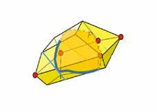
Step 3.2: Clustering of domains

Applying a clustering algorithm requires a metric that can be used to assess the similarity of domains. The clustering of the 8760 domains is based on their geometrical shape by means of comparing the Euclidian distance between vertices. A pre-cluster data split is applied to reduce cluster groups size and hence computational complexity whilst respecting time-related trends. In this split, summer and winter domains are separated, weekends and weekdays are separated, and within the weekdays, the peak and off-peak hours are separated as well. This resulted in the creation of 6 groups to be clustered individually.

Next, the number of centroids to retain are defined. For weekends, one centroid is calculated to represent the entire group, whereas for weekdays, per group, 2 clusters are created, each with its own centroid (see Figure L-10). The clustering was performed by means of a k-medoid algorithm. Here the centroids were elements which were part of the initial domains, and therefore had physical meaning. This process was performed in two steps in order to be able to reduce the set and ultimately find the representative centroids.

The level 1 clustering produced a first set of medoids that were further refined in level 2 in order to reach the targeted number of clusters.

Step 3.3: Resizing and approximating the domains for computational efficiency

The domains are subsequently restored back to their full dimensions of 12 Core biding zones + ALEGrO + (if applicable) AHC dimensions prior to plugging them back into the Antares model. In general, the number of CNECs in the framework’s domains is too large to be of practical use in market simulations.

A flow-based domain is defined by a certain number of inequality constraints representing the limits of critical network elements at a given time. Keeping the complexity at an acceptable level is key to successfully carry out the simulations. A simplification algorithm is therefore chosen based on the Manhattan distance of two hyperplanes. This step allowed the identification of the smallest set of CNECs that could be used to describe the entire domain, without any loss of quality or representativeness. Finally after this step, the final set PTDF-RAM linear constraints where defined and set into the model.

L.4.4. STEP 4: INCORPORATING MULTIPLE FLOW-BASED DOMAINS INTO ADEQUACY ASSESSMENT

The ‘Monte Carlo’ approach used in this study generates multiple possible future states, called ‘Monte Carlo’ years. The method used for relating Flow-based typical days to the climatic conditions within the different the ‘Monte Carlo’ years was originally developed by the French TSO RTE (see reference documents [ANT-3] and [ANT-4]), was also implemented in RTE’s adequacy study (Bilan Prévisionnel since 2017 [RTE-2]), as well as in the Pentalateral Energy ForumGAA 2020 Report (PLEF 2020).

This method can be understood as follows. The k-medoid algorithm not only selects the representative domains for each of the clusters, but also identifies for each day the cluster to which it belongs. Thus, for the climatic variables in scope, thresholds can be defined (typically at the 33rd and 66th percentiles) which lead to the creation of climatic groups. As such, it is possible to identify, for every day, the

climatic group to which it belongs. By counting the amount of times a domain appears in a specific climatic group, it is possible to define a probability matrix. This matrix represents the probability of being in a given cluster of domains under certain climatic conditions. Using the climatic conditions encountered at a given hour in the model, clusters can then be mapped back to the hours in the model. It is this interpretation that is used when mapping the typical days onto the ‘Monte Carlo’ years.

This kind of systematic approach makes it possible to link specific combinations of climatic conditions expected in future target years, e.g. high/low wind infeed in Core (Germany, France...) or high/low temperature and demand in France and Belgium, with the representative domains for these conditions.

FIGURE L-9 — FLOW-BASED DOMAIN – SMART SLICING

FIGURE L-10 — FLOW-BASED DOMAIN CLUSTERING PROCESS

L.5. EVOLUTION OF THE FLOW-BASED METHODOLOGY

Elia is a pioneer in the flow-based approach for adequacy studies and has developed a methodology to model exchanges between countries in the capacity calculation region that replicates the day-ahead operation. In fact, NTC only modelling of exchanges has not been used since 2015 and the introduction of flow-based methodology in CWE. In the first flow-based assessment of winter 2016-17 (the strategic reserve volume evaluation published end of 2015) only one domain was used to represent the entire winter. That domain was based on an historical situation. Since then, leading up to the present study, Elia has since improved its modelling by:

• adding more historical domains;

• relating the domains to the climatic variables in a systematic way;

• incorporating minRAM evolutions within those historical domains;

• correcting historical domains for historical grid outages;

• correcting historical domains for future grid upgrades;

• integrating the breakup of the DE-AT bidding zone on 1 October 2018;

• recalculating the domains to include the planned HTLS upgrade of the 380-kV Belgian backbone;

• modelling the ALEGrO interconnector, which provides additional freedom for the flow-based domain.

• development a flow-based framework which does not rely on historical data and instead mimics the operational flowbased capacity calculation workflow while allowing calculation of flow-based parameters for market and adequacy (mid- and long term) studies.

• adding the flow-estimation step in the process in which internal controllable elements’ set points are estimated prior to simulating the flow-based process by mimicking the operational behaviour in D2CF;

• integrating the Advanced Hybrid Coupling (AHC) for any external border to the CCR considered (e.g. Core); Finally, for the present study, the following additional improvements were added:

• integration of a dynamic allocation constraint for the polish bidding zone;

• combination of AHC and SHC modelling in the same domains to better take into account the specificities on the Channel interconnectors.

M. METHODOLOGY FOR THE ASSESSMENT OF SHORT-TERM FLEXIBILITY

This appendix details the methodology for the assessment of short-term flexibility.

M.1. INTRODUCTION

M.1.1. DEFINITION OF POWER SYSTEM FLEXIBILITY

Although many definitions exist in the literature, the flexibility of a power system is generally defined as: the extent to which a power system can modify electricity production or consumption in response to variability, expected or otherwise’, [IEA-7] has defined by the International Energy Agency. Note that newer definitions add characteristics of reliability and cost-effectivity to this definition, as well as stressing the range of timescales from instantaneous stability to long-term security [IEA-8]. As shown in Figure M-1, power systems and markets need flexibility to cope with three types of uncertainty (also known as ‘flexibility drivers’), as outlined below.

(1) The variability and uncertainty of the demand: it is not possible to know beforehand the exact electricity demand, as it depends on external variables such as consumer preferences and weather conditions. Nevertheless, short-term demand forecast tools are used by market parties and system operators to predict the demand on a week-ahead, day-ahead and intra-day basis to schedule their portfolios and manage their operations.

(2) The variability and uncertainty of renewable and distributed generation: renewable generation such as wind and solar power is characterised by uncertainty, as it is subject to variable and uncertain weather conditions. This is also the case for some distributed generation sources which face variable generation profiles, such as combined heat and power or run-of-river hydro following consumer preferences or weather conditions. Dedicated forecast tools are used by market parties and system operators to predict variations as accurately as possible on a day-ahead and intra-day basis, in order to schedule their portfolio and manage their operations.

(3) Unexpected outages of generation units or transmission assets: forced outages are an inherent characteristic of generation and transmission systems and are unpredictable. They result in the sudden loss (or excess) of power. Forced outages in decentralised generation sources are generally less of an issue due to their dispersed nature, and are typically included in the variable or distributed generation profiles.

• Generation units

• Demand-side assets

• Electricity storage

• Interconnectors

In order to keep the system in balance, which is an important prerequisite for system security, these expected and unexpected variations in demand and generation must be covered at all times with flexibility sources, also referred to as the flexibility means of the system. These are delivered by technologies which are controllable, i.e. can alter their generation or demand upon request in a relatively short time frame. These capabilities can be provided by the technologies outlined below.

(1) Generation units: all generation units are flexible to a certain extent, but not all of them are managed today in a flexible way. It is assumed that most conventional thermal units can modify their output within an acceptable time frame. An exception is Belgian nuclear power plants, which are typically operated as base load units (although some temporary output reductions have proven to be possible under certain conditions). Additionally, non-thermal generation capacity can have flexi-

FIGURE M-1 — FLEXIBILITY DRIVERS AND FLEXIBILITY SOURCES

ble capabilities such as renewable generation, which can, when running, regulate its output downward (upward regulation is considered costly, since this would require a capacity reservation and the availability of wind). Combined heat and power (CHP) can have constraints as they depend on heat demand.

(2) Demand side assets: demand units can provide flexibility through modifying its demand following a reaction to explicit signals, or implicitly by reacting to price signals. In this study, these are referred to as consumption shifting and demand response processes respectively. Note that demand side units is generally activated to facilitate demand reductions (a demand increase would imply using more energy than required, which is generally related to electricity storage processes).

(3) Electricity storage: these technologies are generally very flexible and are characterised by an ‘energy’ reservoir with which they can store electricity via another energy carrier, and convert this back to electricity upon request. These technologies face limitations concerning their energy reservoir. Several storage technologies exist, but for the moment the most relevant for Belgium are large pumped-storage units and battery facilities.

(4) Interconnectors which can import (or export) flexibility from / to other regions by means of cross-border

forward, intra-day/day-ahead or balancing markets. Today, the development of a European balancing market is currently underway by means of balancing energy exchange platforms that will facilitate close-to-real-time flexibility exchanges. Note that the availability of this capacity depends on the availability of transmission capacity (besides the availability of the generation, storage or demand response in other countries).

Ensuring that the system flexibility needs are covered is as important as making sure that the installed generation capacity is able to cover the peak demand. Shortages in flexibility will result in emergency measures to avoid frequency deviations and preventive or real-time generation curtailment or demand shedding. On the one hand, flexibility needs have been seen to increase following the increase of renewable generation (e.g. solar photovoltaics) and new demand applications (e.g. electric vehicles). On the other hand, flexibility means are also increasing following the integration of new demand side management (e.g. electric heating) and storage (e.g. batteries) possibilities.

Therefore, the aim of this flexibility study is to investigate if the future power system has sufficient technical capabilities and characteristics to deal with variations in demand and generation.

M.1.2. FLEXIBILITY IN THE ELECTRICITY MARKET

The diagram in Figure M-2 illustrates the main mechanisms of the operation of the current electricity market.

Market players are responsible for balancing injections and offtake in their portfolio. They must currently nominate an energy portfolio one day in advance (day-ahead) and, by moving further closer to real-time, resolve any imbalance in their portfolio. It is therefore necessary for the market to have

sufficient flexibility, both intra-day and real-time flexibility, to compensate for forecast errors in generation, in particular with regard to renewable energy sources and offtake. In addition, the flexibility available in the system must always allow for the loss of power plants (unavailabilities known a day advance, as well as an unforeseen unavailability after day-ahead).

MARKET PARTIES

Day-ahead market

• Each market party nominates its portfolio per hour in balance based on predictions

• This balance is achieved by means of using various flexibility sources, by means of contracts or own flexibility means

Intra-day market

• Restoring the balance based on new forecasts

· by means of intra-day market (until 1 hour before real-time), or

· through own flexibility means

Intra-day to real-time

• Imbalance settlement tariff of Elia gives incentive to restore balance

• Additional deviations (forced outage, wind power variations) can be dealt with bilaterally or by means of own flexibility means

The role of the transmission system operator in managing flexibility is complementary to the market’s role, because it neutralises the residual imbalance between injection and offtake that is not covered by market players. By means of the imbalance settlement tariff, Elia incentivises the market to adhere to their balancing responsibility as much as possible. This imbalance tariff is driven by the cost of activating balancing energy to resolve the residual system imbalance, both in an upward (to deal with energy shortage) and downward (to deal with energy surplus) direction. Due to this ‘reactive’ balancing mechanism, a large part of the required flexibility

is delivered by intra-day markets and real-time actions and not by Elia.

TSOs use reserve capacity to cover the residual system imbalance as represented in Figure M-3. If an imbalance in the system occurs, this results in an increase or decrease in system frequency. Because the control zones of the ENTSO-E network - also called the Load Frequency Control (LFC) blocks of which the Elia LFC block represents the Belgian geographical area - are connected, a frequency disturbance impacts the entire synchronous zone.

FIGURE M-3 — ACTIVATION PROCESS OF ELIA’S RESERVE CAPACITY

ELIA

Real-time balancing

• Elia manages the residual aggregated system imbalance with imbalance netting with other regions, with ancillary services (aFRR and mFRR), with non-contracted energy bids from market parties

FIGURE M-2 — TIME HORIZONS FOR FLEXIBILITY

The Frequency Containment Reserve (FCR) must restore the balance between the power provided and the power supplied. It is used to stabilise the frequency at a level greater or smaller than the initial frequency, rather than balancing the Elia LFC block. BOX M-1 explains how the required FCR volume is dimensioned by ENTSO-E at European level and allocated to the relevant LFC blocks.

The Frequency Restoration Reserve (FRR) must free up the FCR of the synchronous zone to prevent network instability, or even a failure of the entire electricity system, in the event of additional system imbalances. Each control area is therefore obliged to maintain its balance which is monitored by means of quality criteria assessing the Area Control Error (ACE), i.e. the real-time deviation between measured and scheduled cross-border exchanges on a quarter-hourly (and even on a minute-by-minute) basis.

Unlike the FCR, the FRR ensures that the frequency in the synchronous zone is restored, and that the control zone is re-balanced. The automatic FRR (aFRR) is mainly used to compensate for short and random imbalances. The manual FRR (mFRR) serves as compensation for long, persistent and/ or very extensive imbalances.

• aFRR must be activated automatically within 30 seconds and must be fully available within 7.5 minutes. This is due to be reduced to 12.5 minutes from 2024 onwards.

• mFRR is manually activated and must be fully available within 15 minutes. This is due to be reduced to 12.5 minutes from 2024 onwards.

The required capacity of FRR is determined by Elia as explained in BOX M-1.

BOX M-1 – DIMENSIONING PROCESS OF RESERVE CAPACITY

The required FCR volume is dimensioned by ENTSO-E for the synchronous area of continental Europe. It is calculated on the largest contingency, currently the loss of 3000 MW, complemented by a probabilistic analysis. This volume is allocated to the corresponding LFC blocks according to their weight (in terms of consumption and generation) in the synchronous zone. The methodology is specified in the synchronous area operational agreement and is approved by all relevant regulators [ELI-12].

The FCR capacity for Belgium is 88 MW in 2023.

The required FRR capacity is dimensioned by Elia for its LFC block. First, the needs are determined with a methodology presented in the LFC block operational agreement [ELI-20], subject to a public consultation and approval from the CREG. Since February 2020, this methodology has been based on a dynamic methodology with which Elia determines the up- and downward FRR needs each day based on a calculation of the imbal-

ance risk. This risk is derived from historic observations of system conditions and LFC block imbalances with the help of machine learning algorithms. Results vary from around 1039 MW for upward FRR (rated power of the largest nuclear unit), and up to 1044 MW for downward FRR (rated export power of the Nemo Link interconnector). Note that the up- and downward aFRR needs are currently fixed ‘symmetrically’ at 117 MW, although the implementation of a new ‘dynamic’ methodology is currently under approval by the regulator. The up- and downward mFRR needs are calculated as the difference between the total FRR needs and the aFRR needs.

The volumes are thereafter allocated towards different products for balancing capacity: aFRR and mFRR standard and mFRR flex. No downward mFRR is contracted at the moment. This allocation takes into account the availability of shared FRR reserve capacity with other TSOs and non-contracted energy bids.

M.1.3. SCOPE AND OBJECTIVE OF THE FLEXIBILITY STUDY

As outlined in Figure M-4, this flexibility analysis focuses on the flexibility required between the day-ahead and the realtime in order to ensure the balance in the Belgian LFC block. The flexibility analysis therefore focuses on short-term flexibility, i.e. the capabilities which are required to cover the expected and unexpected day-ahead and real-time variations in the residual load.

Long-term variations (yearly, seasonal, daily) are also referred to as flexibility, but are already covered in the economic dispatch simulations. These variations are taken into account through Monte Carlo simulations representing demand and

renewable generation profiles, as well as the availability of the thermal fleet and transmission assets, representing the market schedules under perfect foresight with an hourly resolution. Note that a long term outlook becomes more important as the share of variable renewable generation continues to grow and renewable generation replaces more of the conventional controllable capacity. Indicators related to a lack of flexibility are typically expressed in terms of expected generation curtailment and lead to discussions on the integration of new technologies such as power-to-gas technologies and sector coupling.

STUDY

Long Term Day-ahead Intra-day Real-time Intra-day to Real-time

The flexibility study focuses on expected and unexpected variations of the residual demand, as well as generation and transmission asset outages, after the day-ahead time frame. The residual load is defined in this study as the electricity demand minus generation from variable renewable energy sources (wind, solar and run-of-river hydro-electric plants following weather profiles) and, other ‘must run’ decentralised generation (combined heat and power and waste incineration following operational constraints such as heat profiles). Imports and exports via interconnections are not specifically taken into account.

Before the AdeqFlex’19 study, intra-day to real-time variations in the residual load had never been explicitly investigated by Elia. Although the first adequacy and flexibility study in 2016 [ELI-13] highlighted a few characteristics of residual load variations, it mainly focused on estimating the required balancing capacity, and did not investigate in detail whether the system is able to cover:

1. unexpected variations following forecast errors and forced outages in real time;

2. forecast updates between day-ahead and real time,

3. 5-minute variations in real time.

By only focusing on the future availability of reserve capacity, this would implicitly assume that part of the flexibility to be delivered by the market is by default available in the system. Obviously, this is not necessarily the case. This may result in an underestimation of the impact of the required capacity

and flexibility of the system. The proposed methodology in this study therefore focuses on the total flexibility in the system.

Figure M-5 shows the relationship between the flexibility study and the adequacy study. In a first step only on the total flexibility needs required between day-ahead and real-time are calculated. The approach did not determine whether it is the market or the TSO which has to cover the required flexibility.

This split is then investigated in a second step by means of making projections on the reserve capacity needs for FCR and FRR to be foreseen by the TSO. The availability of these reserve capacity needs are modelled in the economic dispatch simulations to ensure minimum flexibility requirements, during scarcity risk periods. Note that the share of reserve capacity depends largely on the future ability of market players to cover demand and generation variations. Projections are based on assumptions on market performance, and real reserve capacity requirements are only determined by the TSO closer to real-time based on the observed system imbalances.

As the focus of the flexibility needs modelling in economic dispatch simulations is on scarcity situations, the third step studies the total flexibility available in the market by post-processing the results of the economic dispatch simulations. These available flexibility means are then compared with the required flexibility needs to analyse and prepare for potential challenges.

FIGURE M-4 — SCOPE OF THE ADEQUACY AND FLEXIBILITY STUDY ADEQUACY

M.2. METHODOLOGY TO DETERMINE THE FLEXIBILITY NEEDS

The flexibility needs assessment is based on a categorisation of three types of flexibility (see Figure M-6), derived from the time frame that new information is received by the market players. This may relate to forecast updates, or information concerning the unexpected unavailability of a power plant.

• Slow flexibility represents the ability to deal with expected deviations in demand and generation following the intraday forecast update. It concerns information received between the day-ahead market (up to 36 hours before real-time) and the intra-day forecast received several hours before real-time, depending on the forecast service. Additionally, this flexibility deals with power plant or transmission asset outages which are announced several hours before real-time (or still not resolved after several hours). This flexibility can be provided with most of the installed capacity, as there are several hours to change the output of a generation, storage or demand unit and even start or stop a power plant.

M.1.4. BEST PRACTICE

Best practice based on studies published by TSOs, utilities, energy agencies, research institutes and academic papers reveal few contributions which facilitate a direct implementation of the methodology in Belgium. Most studies focus on the integration of new technologies, such as batteries or demand side management, or on modelling the ideal generation mix for a region given the increasing share of renewable integration. Only a few TSOs have published long-term flexibility studies.

However, the general impression is that most TSOs have only recently started looking at the issue given the increase in renewable generation. Recent studies in Europe and around the world confirm that flexibility is becoming a crucial area for system adequacy. ENTSO-E provided some first insights into flexibility in one of the previous MAF reports [ENT-9]. At this stage, the literature puts forward three general types of approaches:

1. Quick estimates determine some key figures and metrics concerning the flexibility required and the flexibility installed in a system. This may concern an overview of the installed capacity of controllable thermal plants, pumped-storage, demand response and interconnectors; or an analysis of the largest possible power variation in the system. Such approaches, certainly in combination with visualisation tools, allow and provide a comprehensive overview and first understanding of future issues, and allow benchmarking with other regions. However, they do not accurately specify future flexibility needs, and test their availability in the system. A few examples can be found in [NRE-2].

2. Residual load analyses make it possible to assess flexibility needs without a dispatch model - instead these are based on historical variations and forecast errors of demand and variable renewable generation. This is based on a time series analysis of historical data which demands a lot of data (i.e. the availability of at least one year of historical observations and predictions). Maximum variations and forecast errors can be used as metrics allowing them to be cross-checked with available system capabilities. Examples can be found with the Finnish TSO [POY-1], as well as recent academic literature [RTE-5].

3. Modelling flexibility in system models allows flexibility to be specified in unit commitment and economic dispatch models and is used for adequacy studies such as the one used by Elia. This integrated approach is obviously the most complex in terms of mathematical efforts (e.g. impact on computation time) and requires the introduction of new criteria to represent the lack of flexibility (e.g. ramping margins, insufficient ramping resource expectations). The results depend strongly on the level of detail according to which the flexibility needs are modelled (e.g. resolution, time horizon). Examples of such an approach can be found in the academic literature [RTE-5]. Recently, the International Renewable Energy Agency presented a study based on such approaches [IRE-1]

The methodology used by Elia combines elements of the aforementioned approaches: an assessment of the flexibility needs based on historical data and an assessment of the available flexibility based on the outputs of its economic dispatch simulations. With this approach, Elia used a new methodology based on current best practice. This approach can be improved and adapted in future, based on feedback from stakeholders and analysis following implementation.

• Fast flexibility represents the ability to deal with unexpected power deviations in real time, or deviations for which information is received between the last intra-day forecast and real-time. It concerns information received between several hours up to a few minutes before real-time, depending on the forecast service. Additionally, this flexibility type needs to deal with forced outages up to several hours until the providers of slow flexibility can take over.

Fast flexibility can be provided through generation units which are already dispatched and able to modify their output program within a few minutes, or through units which

have start or stop time of a few minutes, as well as storage units (pumped-hydro and batteries) and types of demand side management which are considered very flexible.

• Ramping flexibility represents the ability to deal with realtime variations in the forecast error and in particular the forecast errors of the last intra-day forecast before realtime. It can be expressed as the capacity required for up to 5 minutes, or even per minute (MW/min). Note that, due to the availability of higher resolution data for offshore wind power generation, it recently became possible to increase the resolution to 5 minutes. This type of flexibility does not cover forced outages which are assumed to be covered by FCR, and relieved by fast and slow flexibility. Ramping flexibility is to be covered by assets which can follow forecast error variations on a minute-by-minute basis and therefore only those units which are already dispatched, as well as some battery storage and demand side management units which are considered very flexible.

The split between slow and fast flexibility is set at 5 hours before real-time. This is determined based on:

• the timing of the intra-day forecast update. Different intraday updates are available at predefined moments during the day, depending on the forecast service. As shown in Figure M-6, the most recent intra-day forecast used by Elia is taken as a reference value to make the split between fast and slow flexibility. Currently, this forecast update arrives between 15 minutes and 5 hours before real-time, depending on the forecast service.

FIGURE M-6 — TYPES OF FLEXIBILITY

• the technical limitations concerning the start-up time of a unit. In general, most units can start up in a time frame of several hours, allowing them to deliver slow flexibility. However, some units can start up within few minutes. These can therefore deliver fast flexibility even when not being dispatched. As shown in Figure M-6 the split between slow and fast flexibility is set at 5 hours before real-time, which relates to the start-up time of an existing CCGT unit.

The flexibility needs for each type of flexibility is determined in three steps by:

(1) determining the probability distribution of the forecast errors of the demand, renewable and distributed generation, aggregated as the residual total load forecast error;

(2) determining the probability distribution of the forced outage of generation units and certain transmission assets;

(3) determining the flexibility needs based on a convolution of both probability distribution curves.

This analysis is represented in Figure M-7. It is conducted for each future year based on an extrapolation of the relevant time series by means of the demand and generation capacity projections towards that year.

M.2.1. STEP 1: RESIDUAL LOAD FORECAST ERROR

The residual load is already defined in Section M.1.3 and represents variability both due to total load and generation. This corresponds to the part of the load (positive or negative) to be covered by different means of flexibility, in particular the flexible generation units, purchase and sale of electricity through interconnections, demand management and storage. The calculation of the residual load is based on the assumption that the energy injected by renewables (wind and solar) or the offtake by the demand is not yet impacted by the activation of flexibility. However, it is important to note that production from variable renewable energy sources, as well as the demand side in itself has a potential to contribute to providing flexibility. This is taken into account during the assessment of the available flexibility means.

Figure M-8 illustrates the spread between the residual load and the total load for a day with high renewable generation, and a day with low renewable generation:

• The total load includes a time series based on all the electrical loads across the Elia grid and in all underlying distribution grids (and also includes electrical losses). It is estimated based on a combination of measurements and scaled-up values of injections from production units, including production in distribution networks, to which imports are added. Export and energy used for energy storage are then deducted.

• The residual load subtracts the renewable and decentral ‘must run’ generation from the total load. These profiles include a separate time series per technology for onshore wind, offshore wind, solar photovoltaics and decentral generation. The latter aggregates the production of different decentral production sources including CHP, Run-of-River hydro and waste incineration.

A database is constructed, representing a representative time series of historical real-time production / load estimations, intra-day forecasts and day-ahead forecasts for the total load, wind onshore, wind offshore, photovoltaics and must run generation. The databases are based on data generated by the forecast tools Elia makes available for the market and is further discussed in Section 3.8.1:

• Error Last versus Day-Ahead forecast (Error LF – DA), representing the historical forecast error [MW] between the day-ahead (DA) and the last forecast (LF);

• Error Real-time versus Last forecast (Error RT – LF) representing the historical forecast error [MW] between the last forecast and the real-time (RT) estimations (or observations),

• ∆ (delta) Error RT-LF, representing the historical forecast error variations [MW] of the Error RT – LF between two subsequent periods of 5 minutes.

Note that the first two time series originated from 15-minute time series, while the last time series used the available high resolution time series of the offshore wind power combined with 5-minute interpolations for the other time series for the real-time estimations. The forecasts are kept on a 15-minute basis.

FIGURE M-7 — SCHEMATIC OVERVIEW OF METHODOLOGY TO DETERMINE THE FLEXIBILITY NEEDS

FIGURE M-8 — ILLUSTRATION OF THE DAY-AHEAD PREDICTION OF TOTAL LOAD AND RESIDUAL LOAD FOR A DAY IN JUNE 2025 (LEFT) AND JANUARY 2025 (RIGHT)

Figure M-9 illustrates these profiles for a day in June. It also shows that the intra-day forecast does not always result in a better forecast (although it does on average) which may result in opposite forecast errors for the day-ahead and intra-day. Additionally, it highlights how sometimes, the forecast errors of different technologies smoothen each other out, and reinforce each other during other periods. All time series values are expressed as a percentage of the monitored capacity (the demand is expressed in terms of the average demand, the renewables and must run generation in terms of installed capacity). This enabled Elia to extrapolate the time

M.2.2. STEP 2: FORCED OUTAGES

The probability distribution curve of the forced outages is created for fast and slow flexibility needs. The probability distribution is based on a time series generated with a ‘Monte Carlo’ simulation, taking into account the generation fleet and relevant HVDC interconnectors for the year for which the simulation is conducted in accordance with the following parameters:

• The maximum generation capacity or transmission capacity of relevant generating units and interconnectors: the maximum capacity is aligned with the adequacy study assumptions. Note that until 2030 only Nemo Link is considered relevant, as other interconnector outages result in an import or export via other electrical paths (which is foreseen when calculating operational margins). This is not the case with Nemo Link, since it is the only electrical connection between Belgium and the United Kingdom. As from 2030,

M.2.3. STEP 3: CONVOLUTIONS AND DETERMINATION OF THE FLEXIBILITY NEEDS

In this final step, for each time horizon investigated, the probability distribution curves representing the forced outage risk and the prediction risk are convoluted. This was done for each type of flexibility need:

• Slow flexibility: Prob(Error LF – DA) + Prob(FO24hours)

• Fast flexibility: Prob(Error RT – LF) + Prob(FO5hours)

• Ramping flexibility: Prob(∆t;t-1[Error RT – LF])

This resulted in three new probability distributions per time horizon, for which a reliability level determined the flexibility needs. The 0.1% and 99.9% percentile determined the downand upward flexibility needs. The flexibility needs for every distribution is determined as the percentile of each distribution. This resulted in up- and downward flexibility needs in MW for the period DA/LF and LF/RT but also in flexibility

needs in MW for the delta error LF/RT, which is also expressed as MW/min, by dividing the result by 5 minutes.

A criteria of 99.9% is selected as the trade-off between accuracy and reliability, as there is no legal framework for covering flexibility needs. Choosing the LOLE criteria for both flexibility and adequacy models might have ‘pushed’ the overall reliability criteria below the legal criterion of 3 hours per year. In view of this, a 100% target reliability need to be strived for. However, setting the percentile too high could have made the results too sensitive for extreme events and data problems specific to the historical years considered.

Note that the flexibility needs are considered as fixed. In reality, flexibility needs may vary depending on hour of the day, season and may even be related to other system conditions.

series towards projected values for the period 2024 to 2034. This extrapolation is conducted by means of the installed capacity and demand projections towards 2034, while taking a forecast improvement factor into account (cf. Section 3.8.1).

Finally, the forecast errors are aggregated over the different drivers, resulting in three aggregated time series per time horizon. These are used to build the three probability distributions for each time horizon investigated and for the Error LF - DA, Error RT – LF and the Delta Error RT – LF, used for the slow, fast and ramping flexibility respectively.

Nautilus is added to the exercise, followed by TritonLink as from 2032.

• The outage probability and duration: these parameters are based on a historical analysis of forced outages of different generation types (or HVDC interconnectors). Note that the duration is capped towards 5 hours and 24 hours for fast and slow flexibility, respectively. This is generally below the observed duration, but the slow flexibility is assumed to relieve the fast flexibility after 5 hours (when, for instance, new generation units can be started), and the slow flexibility is relieved by the day-ahead market after 12 - 36 hours.

This also resulted in three probability distributions for each time horizon investigated, taking into account evolutions in the generation fleet (including the nuclear phase-out and the entry of new capacity).

FIGURE M-9 — ILLUSTRATION OF RESIDUAL LOAD FORECAST ERRORS AND VARIATIONS (LEFT) AND THE ERROR RTLF PER FORECAST SERVICE (RIGHT) BASED ON A DAY IN JUNE 2018

M.3. METHODOLOGY TO INCLUDE THE FLEXIBILITY RESERVATIONS

While the previous section assesses the total flexibility needs for the system, this section elaborates on which share needs to be covered by Elia through reserve capacity. A TSO’s objective is to only cover what is needed to ensure system security in line with the European network guidelines, while incentivising market players to balance their portfolios as much as possible. For this reason, the FRR reserve capacity requirements are determined closer to real-time: since 2019, Elia has implemented a dynamic dimensioning method, according to which its FRR needs are determined on a daily basis for each block of four hours of the next day.

As represented in Figure M-10, reserve capacity can be seen as a subset of the fast and ramping flexibility. When establishing a link between the reserve capacity types and the flexibility types, the fast flexibility will contain the future FRR (aFRR + mFRR) needs, which shall be at maximum contracted power in 12.5 – 15.0 minutes. However, the ramping flexibility will contain the future aFRR, which shall be able to react in 5.0 – 7.5 minutes. Slow flexibility is assumed to be covered by means of intra-day markets. Note that the FCR falls outside the three flexibility categories and should be seen as a separate category, dimensioned on the level of the synchronous area of continental Europe and therefore considered outside the scope of this national flexibility study.

The economic dispatch simulations represent the market schedules under perfect forecasts with an hourly resolution. This means all outages and renewable production is known in advance on a week-ahead basis, while forecast variations and unexpected outages within a day are not modelled.

Part of the flexibility needs are explicitly modelled in ANTARES by reserving the FCR and FRR capacity requirements on available generation, storage and demand response assets. This is implemented in line with the ERAA methodology Article 4(6)g [ACE-2]:

“Reserve requirements shall be set separately for FCR, FRR and RR.

i. For each target year, the dimensioning of FCR and FRR, and the contribution of each TSO, shall reflect reserve needs to cover imbalances in line with Articles 153 and 157 of SO GL.

ii. Unless the modelling framework described in paragraph 1(g) is able to model the use of balancing reserves in relation to unforeseen imbalances, FCR and/or FRR (or a part of these balancing reserves) may be deducted from the available capacity resources in the ED […]”

The FCR and FRR reserve capacity requirements are therefore included in economic dispatch simulations by means of additional constraints, which ensure that available capacity in the system covers electricity demand and required reserve capacity needs during periods of scarcity. The adequacy needs of the system are therefore impacted in a way that the system can always cover the day-ahead demand forecast and the balancing requirements (e.g. the loss of the largest power plant). In other words, a capacity meeting the technical requirements of reserve capacity is set aside to cover residual system imbalances. Note that given that this study covers adequacy, only the upward FCR and FRR capacity is taken into account.

M.4. FLEXIBILITY MEANS

After the flexibility needs are determined, and part of the flexibility needs are included in the economic dispatch simulations, the available flexibility means in the system are assessed. It is to be well understood that for sake of efficiency, and to avoid any overestimations of the adequacy needs, the adequacy assessment only integrated reserve capacity requirements during scarcity periods. In other words, it did not take into account the full flexibility needs of the system for every hour of the year. Therefore, the ex post analysis is needed to derive the available flexibility means during non-scarcity periods.

This analysis started from the hourly dispatch of all generation, storage, demand side response units resulting from the

economic dispatch simulations. Taking into account their technical characteristics, the available flexibility from hour to hour is assessed and compared with the required flexibility needs (Section M-2).

Figure M-11 (left) shows that for each Belgian unit, the scheduled output of the unit allows the unit to provide up- and downward flexibility to their minimum stable power and maximum available power respectively. This is calculated for each hour of the climatic years run in the adequacy model. For each hour, the available volume of flexibility from this unit over the period (1 min to 5 hours) is determined.

Available capacity [MW] that can be activated upward in a predefined time period

Ramping flexibility means

• Part of

• FCR is a separate flexibility type, determined at the level of the synchronous area (including N-1 conditions)

As the focus of the economic dispatch simulations is on adequacy and scarcity risk periods, the upward FRR capacity is limited to the dimensioning incident, equal to the capacity of the largest generation or transmission asset with impact on the system imbalance. Note also that given the focus on adequacy, FCR and FRR capacity accounted in the simulations is limited to the upward side.

This is based on its technical characteristics, as outlined in the Section 3.8.3 for the assessment of short-term flexibility:

• for thermal capacity, the plant parameters (maximum power, ramp rate, minimum stable load, start-up / shutdown time, minimum up / down time) are used as well as the hourly power schedule of the units to assess the flexibility that the unit can provide;

• for units with energy constraints (demand side response, pumped storage and batteries, electrolysers), the additional storage limitations are considered in the calculation. The unit provides flexibility (based on its technical parameters, its status on the day-ahead market but also its level of storage or maximum duration of activation) until its reservoir is completely full or empty, or the demand side management. Therefore, their flexibility is limited across time;

• for renewable capacity the ability to deliver downward flexibility potential is considered. This took the limited predictability of this type of generation into account;

• for cross-border flexibility, the remaining available interconnection capacity (ATC) after day-ahead. This capacity is assumed to be available for slow flexibility through the intra-day market. For fast flexibility and ramping flexibility, this capacity is capped by means of different sensitivities to take into account the uncertainty towards the available energy on the balancing energy exchange platforms with which Elia foresees to connect.

Using these results, the amount of up- and downward flexibility each unit can deliver in 1 minute, 15 minutes, 30 minutes, …, (up to 5 hours) is determined. When these profiles are aggregated, this determined for every hour in every ‘Monte Carlo’ year the total flexibility which can be delivered between 1 minute and 5 hours, as shown Figure M-12 (right). Note that these results are compared the required flexibility needs. In order to be able to interpret the results over 8760 hours and several ‘Monte Carlo’ years, the hourly flexibility profiles are further converted into statistics focusing on the available ramping flexibility (5 minutes), fast flexibility (15 minutes) and slow flexibility (5 hours). Note also that the total flexibility expressed the capacity which can be used to cover the fast and the slow flexibility, as shown in Figure M-12. The statistics are compared with the flexibility needs:

• by means of key statistics such as the average, minimum available flexibility, or by means of percentiles expressing the minimum availability (e.g. 99.0% and 99.9%);

• by means of the cumulative probability distribution. The periods 5 hours and 15 min and 5 minute are used as a reference to determine the availability level of total, fast and ramping flexibility. A level of 100% represented a guaranteed availability, while 0% represented that the corresponding flexibility volume is never available in the system.

FIGURE M-10 — RELATION BETWEEN FLEXIBILITY AND RESERVE CAPACITY

the flexibility cannot be covered by the market and results in residual imbalances to be covered by FRR (aFRR/mFRR)

FIGURE M-11 — ASSESSMENT OF AVAILABLE FLEXIBILITY OF ONE UNIT (LEFT) AND AGGREGATED OVER ALL CAPACITY INSTALLED (RIGHT)

FIGURE M-12 — ILLUSTRATION OF THE AGGREGATION OF AVAILABLE FLEXIBILITY (LEFT) AND INDICATORS TO ASSESS AVAILABLE FLEXIBILITY PER TYPE (RIGHT)

I. Electricity consumption in Belgium 423

II. Accounting for recent load reductions in Europe 429

III. Study on the residential and tertiary flexibility by DELTA-EE 430

IV. Study on the forced outage rates by N-SIDE 437

V. Historical availability of the Belgian nuclear units 441

VI. French nuclear historical availability analysis 445

VII. Factors affecting future nuclear availability in France 447

VIII. Socio-cultural measures assumed in the sufficiency sensitivity 449

IX. Additional Adequacy Results 450

APPENDICES ON THE SCENARIO AND DATA

I. ELECTRICITY CONSUMPTION IN BELGIUM

This appendix compiles supplementary information that complements the data presented in Chapter 3 and is utilised to establish the assumptions regarding electricity consumption in Belgium.

I.1. MACROECONOMIC PROJECTIONS

The consumption forecasts for electricity in Belgium take into account macroeconomic indicators derived from the macroeconomic forecasts report published by the Federal Planning Bureau in June 2022.

Figure I-1 illustrates that the outlook presented in June 2022 depicts a more favourable trend compared to the previous year’s forecast. A more recent economic growth projection in February 2023 from the Federal Planning Bureau suggests that economic activity is evolving slightly more positively than anticipated in the previous year. However, it is important to note that this latest projection does not include all the necessary indicators required for the forecasting tool, such as ‘added value per sector’. Therefore, this report’s electricity usage projection relies on the June 2022 report, which could be considered slightly more conservative in terms of GDP growth when compared to the most recent projections, particularly for the later years.

I.2. COMPARISON WITH OTHER STUDIES

The consumption assumed in the CENTRAL scenario for Belgium is compared to other studies and forecasts found. Those are depicted on Figure I-2. Sources include:

• The 'Fit For 55' MIX from the European Commission [EUC-1];

• EnergyVille-Febeliec – Paths 2050 study [ENE-1];

• Ember – Clean Power pathways [EMB-2];

• TYNDP 2024 and ERAA 2023 data collection National Trends+ (NT+) scenario guidance range.

It can be clearly observed that the consumption values assumed in the CENTRAL scenario lie in the range of the different other studies for Belgium.

FIGURE I-1 — OVERVIEW OF THE RECENT PROJECTIONS OF BELGIAN GDP PUBLISHED BY THE FEDERAL PLANNING BUREAU

FIGURE I-2 — TOTAL YEARLY ELECTRICITY CONSUMPTION FOR BELGIUM IN THE CENTRAL SCENARIO COMPARED TO OTHER STUDIES

I.3. ADDITIONAL ASSUMPTIONS REGARDING ELECTRIFICATION OF MOBILITY

The table below outlines the underlying assumptions used to define the various trajectories for the adoption of electric vehicles in road transport. These trajectories are determined based on different annual sales volumes and the corresponding proportions of electrification within those sales.

TABLE I-1 — ADDITIONAL INFORMATION REGARDING THE ASSUMPTIONS ON ELECTRIFICATION OF MOBILITY IN THE CENTRAL SCENARIO AND THE ASSOCIATED SENSITIVITIES

I.4. ADDITIONAL ASSUMPTIONS ON ELECTRIFICATION OF HEAT IN BUILDINGS

Additional assumptions on the quantification of the trajectories for heat pumps are presented in this section. A zoom is made on the development of heat pumps in the residential sector as it is the key sector for the development of heat pumps. Additional assumptions on the development of heat pumps in the tertiary sector can also be found in Table I-2.

The assumptions on the future evolution of the number of heat pumps in the residential sector towards 2035 depend

on the number of new buildings, renovations and old heating systems being replaced, as each of these situations are considered as an opportunity for the installation of a heat pump. As such, the following assumptions are made:

• The number of new dwellings per year is assumed to remain constant until 2035, with 55k dwellings being added each year, corresponding to the previous 5-years average [STA-1] as illustrated on Figure I-4;

The resulting yearly electricity demand associated to those trajectories is presented in Figure I-3.

FIGURE I-3 — ANNUAL ELECTRICITY DEMAND FOR ROAD TRANSPORT IN THE CENTRAL SCENARIO AND THE ASSOCIATED SENSITIVITIES

• The renovation rate is assumed to increase from around 0.7% today [STA-1] to 1.2% in 2035;

• For existing oil and gas boilers it is assumed that 5% are replaced yearly which more or less reflects a lifetime of 20 years.

In terms of share of heat pumps in new sales, the following assumptions are made:

• Today, full-electric heat pumps are mostly installed in new buildings. For Flanders it is assumed that by 2025 all new

buildings will be equipped i) either with a fully electric heat pump (96%) or ii) district heating (4%) due to the phase-out of new gas connections in this region [ODE-1]. For Wallonia and Brussels no strict obligations are yet in place, and it is assumed that 100% heat pump and district heating would be reached in 2035 for new buildings. As 75% of new buildings are nowadays constructed in Flanders, its policies are they key driver for electrification in this segment (see Figure I-4).

FIGURE I-4 — HISTORICAL EVOLUTION OF THE YEARLY NUMBER OF NEW DWELLINGS PER REGION

FIGURE I-5 — ASSUMED HEATING APPLIANCES INSTALLED IN NEW DWELLINGS

Key assumptions for the definition of the LOW, CENTRAL and HIGH trajectories

The underlying assumptions for the definition of the different trajectories for heat pumps are listed in Table I-2. In general, the trajectories are defined by assuming different yearly

new building and renovation rates and the relative shares of heat pump installations.

TABLE I-2 — ADDITIONAL INFORMATION REGARDING THE ASSUMPTIONS ON ELECTRIFICATION OF HEAT IN THE CENTRAL SCENARIO AND THE ASSOCIATED SENSITIVITIES

• For renovations and end-of-lifetime boiler replacements, none of the regions has currently put in place a strict ban on the usage of fossil gas. Therefore, replacement of heating systems by heat pumps is assumed to increase modestly

with 23% in 2030 and 35% in 2035 for renovations, and 20% in 2030 and 27% in 2035 for residual end-of-lifetime boiler replacements (see Figure I-6).

FIGURE I-6 — ASSUMED APPLIANCES INSTALLED IN THE REPLACEMENT OF OIL AND GAS BOILERS REACHING END OF LIFETIME (LEFT) AND FOR RENOVATED DWELLINGS (RIGHT)

The resulting amount of heat pumps is presented in Chapter 3, Section 3.3.4.3. The associated yearly electricity demand for the CENTRAL scenario and HIGH/LOW sensitivities is presented in Figure I-7.

FIGURE I-7 — ANNUAL ELECTRICITY DEMAND FOR HEAT PUMPS IN THE DIFFERENT SCENARIOS

I.5. ADDITIONAL ASSUMPTIONS REGARDING ELECTRIFICATION OF INDUSTRY

II. ACCOUNTING FOR RECENT LOAD REDUCTIONS IN EUROPE

In order to account for the impact of load reductions in 2022 and because no consolidated data or projections were available at the time of constructing the scenarios, Elia performed an analysis of the 2022 electricity consumption in all European countries. The realised demand for 2022 is then used as the starting point to build the ‘short-term’ demand trajectories for this study (2022-2025). Indeed, rather than using outdated shortterm load projections from studies not accounting for the impact of the load reductions in 2022, Elia updated the short-term load projection by considering the 2022 demand as starting point of the projection. An interpolation was then performed between the demand in 2022 and the projected demand in 2025 (based on ERAA 2022 data or most recent national studies). Through this interpolation, the load values for 2023 and 2024 are obtained.

To estimate electricity consumption for European countries without available consolidated 2022 data, the latest data from Eurostat is used (2021) combined with a three-step approach. First, the historical Eurostat data are normalised using Heating Degree Days (see the methodology Appendix B on the normalisation of the load for more information). Secondly, the ENTSO-E Transparency Platform (ETP) realised data for 2021 and 2022 are normalised. Finally, the difference between normalised 2021 and 2022 loads using ENTSO-E TP data is applied on the Eurostat data of 2021.

It is important to note that normalising electricity consumption based on Heating Degree Days requires the estimation of the thermosensitivity of electricity consumption, i.e. know-

ing what is the effect of the temperature on the electricity consumption, which varies from one country to another (e.g. a country with a high share of electric heating such as France will have a higher thermosensitivity). Elia estimates the thermosensitivity of the different countries using the total load data from the ETP and the temperature data of the country between 2017 and 2022 [MET-1]. Figure II-1 illustrates how the thermosensitivity is estimated for France.

Figure 3-78 from Chapter 3, Section 3.5.2.2. shows the difference between the approach considered in this study to estimate electricity consumption in 2022 as explained here and the values of projected demand in 2025 from ERAA 2022 and latest national publications..

Figure I-8 shows the historical and assumed evolution of industrial electricity demand per sector for Belgium in the CENTRAL scenario.

FIGURE I-8 — HISTORICAL AND ASSUMED (CENTRAL) EVOLUTION OF ELECTRICITY DEMAND PER INDUSTRIAL

FIGURE II-1 — DEMAND THERMOSENSITIVITY DETERMINATION FOR FRANCE FOR THE PERIOD FROM 01/01/2017 TO 31/12/2022

III. STUDY ON THE RESIDENTIAL AND TERTIARY FLEXIBILITY BY DELTA-EE

This appendix is a summary of the study performed by DELTA-EE on the residential and tertiary flexibility. The study is also published on Elia’s website [ELI-18]. The study assessed the potential flexibility from different types of electric loads with a focus on new electrified loads such as heating, via heat pumps (HPs) or direct electric heater, and transportation, via electric vehicles (EVs). Several barriers to unlock potential flexibility were identified and quantified in order to assess the amount of devices that could be made flexible in the future.

Many uncertainties remain to know (i) which technologies are interesting to be made flexible (meaning the one consuming most energy, or with the greatest installed power), (ii) the enablers needed to unlock flexibility, (iii) the future forecast of unlocked flexibility. For this reason, Elia hired DELTA-EE (a consulting company) to study the challenges stated here above and cipher future evolution of flexibility in the residential and tertiary sector, to take these into account in this AdeqFlex’23. The study was discussed and presented to stakeholders on 13th and 28th October 2022 and was part of the public consultation on scenarios and methodology in November 2022.

The overall approach is described in Figure III-1. The process of identifying and implementing technologies to deliver flexibility involves several key steps. Here is an overview of these steps:

• Identification of Technologies: The first step is to identify the technologies that have the potential to deliver flexibility on the residential and tertiary consumption side. These also included energy storage systems (such as home batteries), heat pumps, electric vehicles, etc.

• Forecasting Flexibility Capacity: Once the technologies are identified, it is essential to forecast the amount of flexibility capacity they can unlock. This involves assessing the capability of each technology to adjust their output or consumption patterns in response to system needs. For example, batteries can provide rapid response and short-duration

III.1. TECHNOLOGY OF INTEREST

Not all technologies can provide large amounts of flexibility. A few characteristics are needed to make a technology interesting to flexibilise: (i) a large installed capacity relative to the load in the future and (ii) a relatively large capability for flexibility. The latter could be defined as the technical capability to variate its power output, as well as a minimal impact on the comfort of consumers.

Several technologies were reviewed, as summarised in Table III-1. It turns out from DELTA-EE analysis that the most relevant technologies to focus on would be the (i) electric vehicles, (ii) heating loads and (iii) energy storage technolo-

gies. The reader should bear in mind that heating loads are defined by both hot water and space heating.

The amount of electric vehicles and heat pumps installed in the coming years will represent an increasing share of the load in the residential sector, which makes them interesting to flexibilise. It is also worth noting that it is easier to flexibilise new assets being installed, rather than retrofitting existing ones. Then, electric vehicles and energy storage have high capability for flexibility, linked to the technology ramping characteristics as well as their limited impact on the comfort of consumers.

flexibility but are bounded by the amount of energy they can store, while other types of loads can have longer reaction times or other constraints (amount of activations, comfort level...);

• Enablers for Flexibility: Each technology requires specific enablers to deliver flexibility effectively. These enablers can include advanced control systems, communication infrastructure, data analytics, forecasting tools, and regulatory frameworks that incentivise flexibility services. For example, electric vehicles may require sophisticated control algorithms and grid integration capabilities to optimise their operation.

• Integration and Optimisation: The final step involves integrating and optimising the different flexibility assets within the electricity system. This includes developing advanced modelling and optimisation tools to coordinate the dispatch and operation of these assets in a way that maximises system flexibility and efficiency. It also involves market mechanisms that incentivise the provision of flexibility services. By following these steps, it is possible to identify the most promising technologies for delivering flexibility, forecast the amount of flexible capacity they can provide, and determine the necessary enablers to unlock their full potential. This process plays a crucial role in designing and implementing flexible electricity systems that can adapt to the changing needs of the grid and support the integration of renewable energy sources.

Some technologies will not deliver flexibility themselves but rather enable the deployment of flexibility from other technologies. The enabling technologies and the framework developed by DELTA-EE will be covered in following sections. Notably, smart meters allowing more granular metering for consumption are one of the technologies required to unlock flexibility.

Other loads were disregarded from the scope of the study. These include: (i) cooling loads and (ii) miscellaneous loads. The former covers air conditioning systems, and the latter concerns house appliances such as freezer, refrigerator, and lightning.

For cooling loads, the main argument was the lack of data to analyse, as well as the relevance for adequacy. The adequacy issues happening in winter when the air-conditioning is not used. Those could be included in future studies.

Then for miscellaneous, it is important to note that not all loads from a household can be considered flexible. For instance, all appliances related to cooking, lighting, audiovisual, IT cannot be considered flexible without impacting the comfort of the user. The appliances to be considered as flexible are cold appliances (refrigerator), dishwasher and water heating. However, with the electrification of heating and transport, the power that this installed capacity represents is rather small. This is represented on Figure III-2, where it is observed that out of the total peak load of the house, the share that this potential flexibility from miscellaneous loadsfalls to an average of 6% while combining several appliances.

FIGURE III-1 — HIGH-LEVEL VIEW OF DELTA-EE’S FRAMEWORK TO DELIVER THE STUDY

TABLE III-1 — RELEVANT TECHNOLOGIES TO ASSESS FOR FLEXIBILITY IN THE RESIDENTIAL AND COMMERCIAL SECTOR

a global system/market perspective. It is described with the subscript 1H

• Smart load profile – 1M: With electricity dispatch changing every day, the most optimal way to operate any asset would be to have it adapting its load depending on the market prices or even in real-time to the RES production. This results in a dispatch guided by market signals noted as the subscript 1M

• Optimised bi-directional exchange of energy – 2H: For certain assets like batteries or certain EVs, energy can be

III.2. OPERATION MODE OF THE DIFFERENT ASSETS

Having identified the technologies relevant to provide flexibility, defining how these assets can be operated is key. A flexible operation of an asset can only happen if the asset receives a control signal. This control signal could have different origin, and DELTA-EE summarised these in two categories: (i) a Local (or House signal) and (ii) a Global (or Market) signal. In the first case, the asset is operated flexibly based on a signal related to the home energy management. The signal could be linked to PV production, or network time-of-use tar-

iffs, and the goal would be to minimise costs. Whereas in the second case, the signal comes from an aggregator or system operator whose purpose are to balance the grid.

The parallel can be made with ‘implicit’ and ‘explicit’ flexibility (these are shown in Figure III-3). The control signal for implicit flexibility is based on avoiding costs (like network or capacity tariff), which could be linked to the local control signal. Whereas control signal for explicit flexibility means to generate revenue, similar to what is described as market signal.

e.g. : time-of-use network charges, or capacity tariffs: system operators incentivise consumers to alter the timing of their consumption in order to reduce grid congestion

The technical characteristics of the asset could also be impactful on the definition of the operation mode, for instance the ability to inject energy back to the grid (such is the case for EVs and batteries).

Overall, the following categories for all assets were defined:

• Natural load – 0: This load profile represents the current operation of the asset without considering optimisation for grid management, price clearing, or renewable energy inte-

e.g.: ancillary services: system operators pay for active frequency control Tomorrow?

gration. It serves as a baseline and is denoted by the subscript 0

• Optimised load profile – 1H: With relevant network tariffs or appropriate market reforms, virtuous behaviours in regards to the grid could be incentivised (e.g. flatten the load by minimising peak load, consuming outside of peak hours, maximising self-consumption of PV's…). It aims to flatten the load and is guided by a local signal. However, it may not represent the most optimal way to operate the asset from

exchanged in two directions. This has the potential to not only move the load outside of peak hours, but also inject electricity back into the grid during these peak hours. When this operation happens after following a local signal, it is defined by the subscript 2H

• Smart dispatch of virtual power plant – 2M: With proper market reforms and infrastructure, the bi-directional assets could be dispatched by the market. Similarly to the 1M subscript, this is described as a 2M subscript with the only difference residing in the ability to inject electricity back into the grid, on top of moving the load outside of peak hours.

TABLE II-2 — SUMMARY OF OPERATION MODES AS DEFINED BY DELTA-EE

CONTROL SIGNALS

H - House Signal

Operation of asset based on a Local signal from the household

E.g.: Static & Dynamic time of use tariffs, capacity tariffs, PV optimisation

Heat-Pumps HP1H Flexible operation - implicit flexibility

V1H Smart charging - implicit flexibility

Electric Vehicles

V2H

Bi-directional smart charging - implicit flexibility

Residential Batteries B2H

Flexible operation - implicit flexibility

The modelling of these operation modes takes into account the technical characteristics of the asset, such as its ramp rate, and also considers the impact on the consumer’s comfort. It recognises that certain assets, like a heat pump, may have the technical capability to shut down, but if it results in an uncomfortable living environment for the owner, it would not be realistic to model this behaviour. Therefore, the model ensures that the operation of the asset remains realistic and within acceptable comfort ranges for the energy end-uses.

These end-user technologies do not only contribute to adequacy through the flexible operation, they also contribute to short-term flexibility in the AdeqFlex’23 study. DELTA-EE covered the capabilities of end-user technology to deliver short-term flexibility. The latter is defined with different timeframes (ramp, fast and slow flexibility). For each timeframe, a different share of end-user appliances can react: less appliances will react to short-term flexibility than for the long-term flexibility. The main underlying constraints lie in (i)

M - Market Signal

Formal contract with the market to provide flexibility

E.g: Ancillary services, Interval balancing, Trading, DSO services

HP1M

Flexible operation - implicit & explicit flexibility

V1M

Smart charging - implicit & explicit flexibility

V2M

Bi-directional smart charging - implicit & explicit flexibility

B2M

Flexible operation - implicit & explicit flexibility

communication with the aggregator running smoothly, (ii) technical constraints of flexibility (e.g. if the compressor of a heat-pump is running) and (iii) the current operation of the appliance (e.g. whether the appliance is on or off). All in all, the share of end-user appliances expected to deliver shortterm flexibility respectively for ramp, fast and slow flex are 50%, 70% and 100%.

Moving forward, the study focuses on identifying the elements required to unlock flexibility, which are referred to as ‘enablers of flexibility’. These enablers play a crucial role in facilitating the delivery of flexibility services by the relevant technologies. They encompass various factors, such as market mechanisms, regulatory frameworks, grid infrastructure, communication systems, and advanced control algorithms, among others. The analysis of these enablers is essential to understand the requirements and conditions necessary to fully utilise the flexibility potential of the identified technologies.

FIGURE III-2 — SHARE OF THE AVERAGE PEAK LOAD FROM APPLIANCES IN A HOME

Non-flexible appliance load Cold Appliances Washing/drying/dishwasher HP EV Water heating'

FIGURE III-3 — DIFFERENCE BETWEEN IMPLICIT AND EXPLICIT FLEXIBILITY DEFINED IN DELTA-EE STUDY

III.3. ENABLERS OF FLEXIBILITY

It is not because an asset is technically able to deliver flexibility, that it will do so. Different barriers need to be overcome before the asset is operated flexibly. These key enablers are summarised Figure III-4.

FIGURE III-4 — SCHEMATIC DEPICTION OF FLEXIBILITY ENABLERS

The key factors are described hereunder:

• Asset Volume: This defines the total installed base and its rated capacity. Factors that incentivise technology deployment or that require technology deployment are the primary enablers. This is detailed in the scenario assumptions of the AdeqFlex’23 study.

• Asset flexibility: Assets have a primary function and demand profile that defines the capability of that asset to provide flexibility in coordination with any inherent energy storage. The demand profile defines the temporal limitations to flexibility and also when increased load is required to compensate for reductions in demand.

- EV: cars being parked most of the time, the main factor impacting flexibility will be the charger availability: whether chargers are available where EVs are parked (at home, at the office, in public parking). Also, not all segments were evaluated fit to deliver flexibility by DELTA-EE. Notably, public charging due to the limited time connection at these locations. Additionally, in the coming years, new cars will be compatible with bi-directional exchange of energy. Now, to know if chargers installed will be compatible, or needs retrofitting, is also another question that needs to be assessed in order to define the flexibility potential to come.

- HP: the flexibility of heat pumps depends on the margin available to pre-heat the house before it is occupied, and let it cool down. This varies depending on the building insulation as well as on each given day where the outside temperature (and heat losses) varies as well.

• Control signal: A local or market signal is necessary to drive the flexible operation of assets. This signal is responsible to adjust the consumption of the asset and variate over time according to the system’s need.

• Control capability: Depending on the required control signal, the asset(s) must have the necessary capability to respond appropriately and optimise performance to meet the necessary flexibility requirements. Note also that communication protocols and standards need to be established. Indeed, standardising exchange of information between devices and ability to control them is also key (e.g. an electric vehicle from a certain brand and using a smart charger from another brand should be allowed to know when is the most appropriate moment to charge based on the home PV generation from another brand).

- HPs: For all assets to deliver flexibility, they will need to be able to receive signals and be automated. It is expected that not many HPs are retrofitted to meet this requirement, but that HPs need to be made smart at conception.

- EV: For EVs, it is the charger itself that needs to be made smart in order to enable smart charging, whether uni- or bi-directional. However, for the latter, a special charger needs to be installed to allow flow of energy in both directions, and these are expected to come only when the appropriate EVs will be sold on the market. In Figure III-5, the reader can see the assumed evolution in the chargers installed in coming years. The vast majority of installed chargers are expected to be made smart (meaning having the capability to charge based on a signal), and also unidirectional as these are linked to uni-directional charging cars. The projection of bi-directional chargers is based on the forecast of EVs sold with the bi-directional functionality. Note that the forecast is built under the assumption to keep a ratio of 1 charger per 2.17 EVs.

FIGURE III-5 — ASSUMED FUTURE EVOLUTION OF EV CHARGERS PER TYPE

Roll-out of bi-directional chargers as new car sales implement the technology, after 2027

The majority of chargers are expected to be installed with smart features

• Appropriate metering: Monetising flexibility requires measuring the dynamic electricity load from the household with sufficient accuracy for the control signal and flexibility service provided. These systems must also be appropriately

connected such that services can be effectively measured and billed by the correct parties. All regions in Belgium have made their plans to roll-out smart meters. The global deployment of smart meters is depicted in Figure III-6.

installing 40k smart meters per year. Wallonia targeted 90k smart meters by the end of 2022. A constant rate is assumed after

of Flemish household covered with smart meters by 2024.

FIGURE III-6 — FORECAST OF SMART METERS ROLLOUT PER REGION IN BELGIUM

• Customer barriers: With control signals and assets available, the complexity of the service offering and the impact on the customer comfort will be the key final barriers to participation in flexibility services before consideration of the scale of customer benefit. The customer barrier will also not be the same for out-of-market flexibility, or in-the-market. In the former, the customer retains more control on their appliances. For this reason, DELTA-EE assumed that the uptake of the latter to be lower (see Table III-3). This is where initiatives like Customer Centricity Market Design of Elia aims to (i) help consumers to engage with flexibility providers and (ii) simplify measurement behind the meter, as well as ease the settlement and financial valuation of flexibility services provided by consumers.

- EV: the main barrier for customer will be regarding their comfort. For EVs, this can take the form of a guaranteed State of Charge that the user can impose for a certain time he or she will need to use their cars.

- HP: the main barrier for customer will be regarding their comfort. This is especially challenging for heating as consumers expect a certain temperature inside their homes. The common way to answer this is to make assumptions on the temperature setpoint of the house. Regarding space heating, the appliance can become flexible only if a range of temperature is considered instead of a setpoint (e.g. heating +- 2°C around a setpoint, instead of a constant setpoint). For hot water, it is assumed that water can be heated with marginal heat losses and no impact on the consumer’s comfort. While the capability of heating technologies is highly sensitive to the season and local assets, the enabling technologies and customer barriers will be critical, with impact on consumer and complexity being the most important barriers to overcome for widespread uptake.

With DELTA-EE’s enablers framework made explicit, the three next sections explain how this has been translated into uptake of the different operation modes for each asset.

IV. STUDY ON THE FORCED OUTAGE RATES BY N-SIDE

This appendix explains the methodology developed by Elia and N-SIDE for the determination of the necessary metrics regarding forced and planned outages used in this study and future adequacy studies performed by Elia. The outage metrics are used in the modelling of generation units, pumped-storage and HVDC links. It is important to note that the forced outages of nuclear units were assessed separately by Elia prior to this study (see Appendix V).

IV.1. OUTAGE RATES IN PREVIOUS ADEQUACY STUDIES

In the framework of the previous AdeqFlex’21, the forced outage parameters were calculated on a yearly basis based on historical data from 2011 to 2020 for Belgian units. The used data was a combination of ENTSO-E Transparency Platform (ETP) data, where available, and Elia’s internal database, where needed.

III.4. RESIDENTIAL BATTERIES

Regarding storage, the residential batteries do not face all limitations that heat pumps and electric vehicles face. They do not have a load profile, or an energy demand to answer to. The purpose of batteries is to provide flexibility to the consumer by definition. It can be then assumed that batteries will provide flexibility once installed. However, the flexibility could be implicit (e.g. optimising PV generation) or explicit (e.g. bid in the market, providing ancillary services).

Note that the use of batteries with PV could be seasonally dependent: their primary role can be to integrate solar PV

While it has low customer impact to optimise selfconsumption according to tariffs, some resistance and disinterest is likely while tariffs are a free choice.

The offer for grid services and potential loss of asset control can be difficult for some customers to understand and it is harder to quantify the customer benefit, therefore uptake is expected to be significantly lower.

in the residential sector in summer, and to provide ancillary services in winter. This way, consumer’s could make sure to recover their investment by maximising self-consumption when their PV produce energy and monetising their asset when they are not producing.

The share of batteries participating to market flexibility is expected to grow with the penetration of smart meters in the system, as well as the presence of market players offering a simple and attractive offer to battery owners.

The method previously used to determine the outage indicators posed some limitations:

• No data is available in ETP data before 2015 and hence both databases had to be combined;

• No ETP data is available for units <100 MW while outage parameters are also required for smaller units;

• Elia’s internal database only provides daily granularity;

• The availability of data for certain technologies in Belgium is limited, which poses a challenge in terms of ensuring statistically robust data. When the number of units is small, it becomes difficult to draw accurate and reliable conclusions based on the available data. Statistical robustness relies on having a sufficiently large and diverse sample size to min-

imise biases which could be driven by one specific unit or event in the past:

- CCGT: 20 units (note that some units are split in GT and ST but are part of the same plant);

- OCGT: 11 units;

- CHP: 27 units;

- TJ: 13 units;

- Pumped storage: 2 units;

- Biomass: 5 units;

- Incineration stations: 13 units.

• Due to the limited dataset, a given year in the past could have a strong impact on the unavailability indicators. Given these limitations, Elia and N-SIDE developed an improved method for estimating the outage parameters for future adequacy studies to be used as from AdeqFlex’23. A public consultation was held in November 2022, as part of the AdeqFlex’23 consultation on methodology and scenarios. In addition, the methodology was presented in a WG Adequacy on 28 October 2022 to the stakeholders.

TABLE III-3 — ASSUMED CUSTOMER UPTAKE FOR A CUSTOMER TO TAKE PART TO IMPLICIT OR EXPLICIT FLEXIBILITY

IV.2. METHODOLOGY

To address the limitations mentioned earlier, outage indicators were calculated using a larger dataset that includes data from other countries. By expanding the dataset and using a standardised database, the analysis becomes more robust and reliable. This approach allows for a broader comparison and benchmarking of outage indicators across different regions. Furthermore, the results obtained from this analysis were compared with values reported in other studies and

IV.2.1. OUTAGE INDICATORS

There are three relevant indicators regarding planned and forced outages. These are the average rate, the average duration and the average number of events (see Figure IV-1).

literature reviews. This comparison helps validating the findings and provides additional insights into the outage parameters. By using a larger dataset and considering findings from previous studies, there is less need for frequent updates of outage parameters in future studies. This approach provides a more stable and consistent framework for assessing outage indicators, reducing the reliance on frequent parameter updates.

IV.2.2. DATA SOURCE ASSESSMENT

In this phase, a list of possible data sources was compiled, and each source was evaluated to determine the most appropriate and reliable data source. Specifically, Elia and N-SIDE assessed Elia’s internal database, ENTSO-E Trans-

parency Platform (ETP) and transparency platforms from producers active in the Belgian electricity market. Table IV-1 summarises the advantages and disadvantages of the various assessed data sources.

TABLE IV-1 — OVERVIEW OF THE ASSESSED DATA SOURCES

Description ENTSO-E Transparency Platform (ETP) [ENT-4] Elia’s internal database

Advantages Legal obligation for units larger than 100 MW to report outages

FIGURE IV-1 — OVERVIEW OF INDICATORS FOR PLANNED AND FORCED OUTAGES

Disadvantages

Large sample size: outage data for all ENTSO-E bidding zones Reporting of partial outages 15-minutes time granularity Public information

No data for units <100 MW

Only data available as from 2015

Following the assessment, it was determined that, when feasible, the ENTSO-E Transparency Platform (ETP) would be utilised, supplemented by Elia’s internal data in the absence of ETP data (for units below 100 MW). While transparency platforms offered by electricity market producers in Belgium

• Outage data on all unit sizes

Producers’ transparency platforms such as NordPool [REM-1], EDF [EDF-1], TotalEnergies [TOT-1], Engie Transparency [ENG-1]

• Data available for more than 10 historic years Reporting of partial outages 15 minutes time granularity Public information

• Only data for Belgium

• Only daily granularity

• Not public information

Mainly data for units >100 MW Different platforms per producer Limited number of years

generally provided similar data to that available on ETP, they only covered a limited number of years and increased the complexity of aggregating multiple data sources. Furthermore, not all producers maintain a data platform, and data on smaller units was scarce.

IV.2.3. DEFINITION OF THE DATA SAMPLE

The indicators from Figure IV-1 should be understood as:

• The planned outage rate is the amount of planned unavailability to the total energy that could have been produced. The total energy that could have been produced is the unplanned unavailable energy + the planned unavailable energy + the available energy (referred as 'Total energy');

• The forced outage rate is the ratio of unplanned unavailable energy to the sum of the available energy and the unplanned unavailable energy;

• Average duration of forced or planned outages;

• Average amount of outages (forced or planned) per year.

Only a limited number of units for each technology exists in Belgium and for some technologies (e.g. CHP) most units are smaller than 100 MW and little ETP data is therefore available. The number of Belgian units considered per data source for each technology is presented on Table IV-2. TABLE

To obtain a larger and more representative sample, the data for Belgium is combined with ETP data for a list of representative other countries for all technologies considered. The outage indicators are calculated on this combined dataset. The other countries considered are:

• France;

• Netherlands;

• Germany;

• United Kingdom;

• Italy.

Since data in ETP is only available as from 2015, the outage metrics are calculated on the time horizon 2015-2021 for the whole dataset, for each data source and each country.

IV-2: REPARTITION OF BELGIAN UNITS BETWEEN DATABASES

IV.2.4. DATA QUALITY AND PRE-PROCESSING

Both ETP and Elia’s internal database were found to contain some data quality issues which were corrected by applying 3 pre-processing steps:

1. Removing duplicate outages: some outages are reported twice for the same period and should therefore only be considered once;

2. Cleaning of overlapping outages: some outages were found to be overlapping with other outages. This would cause outages to be counted twice for some periods.

IV.2.5. LITERATURE REVIEW

The forced outage rates calculated for Belgium and other representative countries were compared with results from other studies on outage rates and the outage rates given by ENTSO-E in the common data for thermal units.

The sources considered in the literature review are:

• The annual system report by Red Eléctrica [REE-1];

• 2021 State of the Market Report for PJM by Monitoring Analytics [MAN-1];

IV.2.6. METHODOLOGY OVERVIEW

Following the analysis steps described in the previous paragraphs, the approach to obtain the final outage indicators is summarised on Figure IV-2.

First, the relevant data was collected from the chosen sources. After applying the pre-processing steps, the data was compared to producers’ transparency platforms. This robust dataset was then used to calculate the necessary indicators for Belgium and other countries. After a comparison

Overlapping outages were therefore split and overlapping periods removed;

3. In case a forced outage is immediately followed by a planned outage, the planned outage is converted to a forced outage. It is assumed that an unexpected forced outage cannot change to a planned outage after a short period of being in forced outage. In the opposite case where a planned outage is followed by a forced outage, no adaptations are made.

V. HISTORICAL AVAILABILITY OF THE BELGIAN NUCLEAR UNITS

This appendix provides more detailed information on how the historical availability of Belgian nuclear units is determined. The historical availability is then used as basis to define the assumed values in the CENTRAL scenario. This appendix aims to complement the information already presented in BOX 3-7.

• 2021 State of Reliability by NERC [NER-1];

• Electricity Capacity report by National Grid [NAT-1];

• Common data used in the ERAA & TYNDP studies by ENTSO-E.

Other sources were consulted as well but provided no clear distinction between unavailability types.

Due to the stringent safety protocols and regulatory framework surrounding nuclear facilities, outage calculations for nuclear units require a more meticulous approach. Indeed,

it is important to be able to distinguish the different type of outages and their associated probability.

V.1. OVERVIEW OF OUTAGE TYPES FOR NUCLEAR UNITS IN BELGIUM

Regarding historical availability of nuclear power plants, four independent and cumulative statuses are defined, considering that forced outages could be split between ‘technical’ and ‘long-lasting’ forced outages:

BOX 3.7). These events are assumed to be independent from climatic conditions and can therefore occur at any time during the year and therefore have an impact on the available capacity during winter.

of the results with the results found in a literature review, the final list of outage indicators was proposed for consultation. The overview of resulting indicators taking into account the feedback from the public consultation can be found in Section 3.4.4.

The full report submitted to public consultation can be found in [ELI-18].

• The unit was available (presented as ‘Available’ in BOX 3.7).

• The unit was in a planned outage A planned outage is considered as usual maintenance but also includes longer planned maintenance periods needed to solve issues encountered after a ‘long-lasting’ forced outage (presented as ‘Planned Unavailability’ in the analysis in BOX 3.7). Regular maintenance is assumed to be performed outside of the critical periods for adequacy even though some planned outage events have been observed during winter when looking at historical data. Some planned outages also need to respect the fuel cycle of the unit and cannot easily be moved. For this reason, an independent indicator on planned outage during winter is integrated in the conclusions. Note that planned outage also includes the long-term operations (LTO) outage periods which are significantly longer than regular planned outage periods as they include additional works to be performed to extend the unit lifetime.

• The unit was in ‘technical’ forced outage. A ‘technical’ forced outage is usually an unexpected event or malfunction leading to the shutdown of the unit to fix a well-defined and limited issue (presented as ‘Technical Force Outage’ in

• The unit was in a long-lasting’ forced outage A long-lasting forced outage is an unpredictable event, leading to a long-lasting shutdown of the unit (presented as ‘Long-lasting Force Outage’ in BOX 3.7). Similarly to ‘technical’ forced outages, these events are assumed to be independent from climatic conditions, meaning that they can occur anytime during the year and therefore impact adequacy in winter. This assumption is confirmed by looking at historical data. Note however that longer planned outages required to fix these long-lasting events are not considered in this category. The split between ‘long-lasting’ forced outage and longer planned outages required to fix those is based on information of the AFNC/FANC website and on a case-bycase analysis on planned outages of the different nuclear units. More details can be found in the section ‘Details on unit per unit type of historical availability events per unit’. In this study, outages for nuclear units are modelled using a four-state Markov chain with the four states being, available, planned outage, technical forced outage, and long-lasting forced outages. A more in-depth explanation can be found in methodology Appendix C.

V.2. DETERMINING OUTAGE RATES

The outage rates for Belgian nuclear units are calculated on historical daily nomination data from 2012 to 2021 for all nuclear units in Belgium.

First, the technical forced outage (TFO) rate is calculated as:

‘Technical’ FO rate = TFO days 2012 → 2021 (TFO days+Available days ) 2012 → 2021

Regarding ‘long-lasting’ forced outages (LLFO), the following formula is used to calculate the corresponding rate:

'Long lasting' FO rate = - ’ Technical’ FO rate (TFO days + LLFO days)2012 → 2021

TFO days + LLFO days + Available days 2012 → 2021

Finally, the planned outage rate is calculated as the planned unavailability on the total period:

PO days 2012 → 2021

V.5. DISCUSSION ON THE RESULTS AND ADDITIONAL CONSIDERATIONS

The results presented above were calculated on historical data for all nuclear units in Belgium from 2012 to 2021.

First, it is important to mention that Doel 4 and Tihange 3 units are the most recent nuclear units in Belgium and hence could experience less outages than older units. However, these units will be extended beyond a 40-year lifetime and will therefore have to undergo LTO works as it was already the case for Tihange 1, Doel 1 and Doel 2. These LTO works could lead to either extended planned outages or ‘long-lasting’ forced outages due to the analysis performed or to the critical operations to be performed. In addition, as it can be observed on the graphs in BOX 3-7 of Chapter 3, ‘long-lasting’ forced outages also happened on the two most recent units.

PO rate =

Total days 2012 → 2021

Note that ‘technical’ forced outages, ‘long-lasting’ forced outages and planned outages should be considered as independent and cumulative.

V.3. EVENTS CONSIDERED AS ‘LONG-LASTING’ FORCED OUTAGES

A defined number of events were considered as ‘long-lasting’ forced outages, based on information available on the AFCN/ FANC website:

1. Indications of microflakes in the nuclear vessel of Doel 3 and Tihange 2 [AFC-1];

2. Doel 4 sabotage [AFC-2];

3. Concrete degradation on bunkers of Doel and Tihange (D3/D4/T2/T3) [AFC-3];

4. Concrete issue during LTO on Tihange 1 [AFC-4]. The unit-by-unit details are presented in ‘Details on unit per unit type of historical availability events per unit’.

V.4. HISTORICAL AVAILABILITY OF NUCLEAR UNITS

By considering both ‘technical’ forced outages and ‘long-lasting’ forced outages on all Belgian nuclear power plants, a forced outage rate of 20.5% is determined:

FO rate = ’Technical’ FO rate + ’long – lasting’ FO rate = 4.0% + 16.5% = 20.5%

Note that the ‘technical’ forced outage rate is in line with the ‘unplanned capacity loss factor’ calculated by the IAEA at world level [IAE-1].

While forced outages are assumed to be independent from climatic conditions and therefore calculated on the whole year (which is confirmed by historical data), planned outages are mainly foreseen outside of winter periods. Elia assumes that no planned outages occur during winter for thermal

units in Belgium (nuclear included) unless those planned outages are already foreseen under REMIT for the upcoming three years. However, as visible on the graphs in BOX 3-7, historical observations show that planned outages also occurred during winter for nuclear units in Belgium.

It is therefore of interest to also analyse the unavailability rate due to planned outages in winter as well, as these can have an impact on adequacy. Therefore, a planned outage rate is calculated on winter periods only:

PO days in winter 2012 → 2021

PO rate = = 8.1 [%]

Total days in winter 2012 → 2021

It is also important to note that average values do not include the discretionary impact that ‘forced long-lasting events’ can have. The occurrence of such an event on Doel 4 or Tihange 3 would result in an entire unit of over 1 GW being unavailable for a long period. This is different when looking at other types of units where there are more units but also generally of smaller size meaning that the impact of an outage is less severe.

Although planned maintenance outages for nuclear units are typically scheduled outside of the winter period to min-

V.6. CONCLUSION

The forced outage rate for Belgian nuclear units considered in the CENTRAL scenario includes both ‘technical’ and ‘long-lasting’ forced outages, resulting in 20,5%

In addition to the forced outage rate there is an additional risk from the planned outage rate during winter of 8.1%. Sensitivities on the nuclear availability assumptions are integrated in this study.

imise the impact on security of supply, it is important to acknowledge that certain circumstances might necessitate maintenance works during winter for nuclear units. Nuclear units may have unique constraints and considerations compared to other thermal units (e.g. fuel cycles), which can influence the scheduling of maintenance activities. In addition, there is no official view on the maintenance works and LTO planning for the two units that are assumed to be extended in the CENTRAL scenario. Such risks are not incorporated in the values used in the CENTRAL scenario (composed of both the ‘technical forced’ and the ‘long lasting forced’ outages) as it is assumed that nuclear extension works and maintenance will be performed outside of critical periods for adequacy. So-called ‘common mode’ failures of units are not explicitly taken into account in this analysis as the values provided only look at averages. Some ‘long-lasting’ forced outage events can have an impact on more than one nuclear unit. Indeed, given the similar design/construction of the two most recent units, any anomaly found in one unit could also be found in the other one. Common mode failures have already occurred several times in Belgium (microflakes, concrete degradation on bunker buildings) but also in France. Combined with the discretionary nature of these events, the impact on the contribution of nuclear units to adequacy is exacerbated.

FIGURE V-1 — OUTAGE RATES [IN %] FOR NUCLEAR TECHNOLOGY

V.7. DETAILS ON UNIT PER UNIT TYPE OF HISTORICAL AVAILABILITY EVENTS

The following section presents an overview of past events affecting the availability of nuclear units during the period from 2012 to 2021.

Events affecting the availability of Doel 1:

• 40-years lifetime ended in February 2015. The unit was then stopped for some months before the political decision was taken to extend its lifetime to 50 years;

• 2 long planned unavailability periods happened from 2018 to Q2 2020 and are linked to the operations and maintenance related to the LTO;

• No long-lasting forced outages were considered.

Events affecting the availability of Doel 2:

• 40-years lifetime was supposed to end in November 2015 but its lifetime was extended to 50 years after a political decision;

• 2 long planned unavailability periods happened from 2018 to Q2 2020 and are linked to the operations and maintenance related to the LTO;

• No long-lasting forced outages were taken into account.

Events affecting the availability of Doel 3:

• 2 long-lasting forced outages are considered in 2012-2013 and 2014-2016 related to the indications of microflakes in the nuclear vessel;

• 1 long-lasting forced outage period is considered from 2017 to 2018 related to concrete degradation on bunkers.

Events affecting the availability of Doel 4:

• 1 long-lasting forced outage period is considered in 2014 due to a sabotage;

• 1 long-lasting forced outage period is considered in 2019 related to concrete degradation on bunkers.

Events affecting the availability of Tihange 1:

• 1 long-lasting forced outage period is considered in 2016 to 2017 due to a concrete issue on a safety building;

• 3 periods linked to the operations and maintenance related to the LTO are considered, including the last one regarding the commissioning of the ‘SUR étendu’ building.

Events affecting the availability of Tihange 2:

• 2 long-lasting forced outage periods are considered in 20122013 and 2014-2016 related to the indications of microflakes in the nuclear vessel;

• 1 long-lasting forced outage period is considered from 2018 to 2019 related to concrete degradation on bunkers.

Events affecting the availability of Tihange 3:

• 1 long-lasting forced outage period is considered in 2018 related to concrete degradation on bunkers;

• 1 long period of planned unavailability considered in 2020 related to extra-work required to repair the concrete degradation on bunkers.

VI. FRENCH NUCLEAR HISTORICAL AVAILABILITY ANALYSIS

This appendix provides an analysis conducted by Elia on the availability of the French nuclear fleet using historical availability data as published by the French nuclear producer. The analysis reveals a consistent pattern of underestimating the planned unavailability of the French nuclear fleet, resulting in a significant number of units being unavailable during winter seasons. This underestimation ranges from 3 to 17 units (of 900 MW), in addition to what was initially forecasted a few months before the winter season. Figure 3-92 of Chapter 3 gives a visual overview of the impact calculation for each winter.

The nuclear unavailability is clearly underestimated in REMIT

In order to evaluate the accuracy of the forecasted French nuclear availability based on REMIT data, a comparison is made between the availability data from the past 8 years and the actual realised availability as reported by EDF. As illustrated on Figure VI-1, there is a clear, structural under-estimation of the unavailability of the French nuclear fleet in the REMIT data published 1 or 2 years in advance when compared to the actual unavailability.

The figure displays the planned unavailability that was known end of each calendar year as well as the realised planned and forced unavailability of the French nuclear fleet. Each curve (in colour) relates to the predictions made at the end of a specific year in terms of expected planned outages for the upcoming 3 years. The black curve represents the realised planned unavailability across the years. The dotted black curve includes the forced outages (on top of the planned

outages already included in the black curve). The difference between the realised planned availability and current forecast (black curve) and the different coloured curves (previous forecasts) is the underestimation of the unavailability.

This analysis confirms that using REMIT availability data without applying a cautious approach is not a reliable method for estimating future French nuclear availabilities. As also indicated in the Chapter 3, the REMIT availability data do not align with forecasted generation by the French producer for future years.

Additionally, this analysis confirms that the availability of nuclear power during winter months in France is progressively decreasing each year. However, the expected REMIT forecasts for upcoming winters still remain at levels observed prior to 2017.

FIGURE VI-1 — FORECASTED VS ACTUAL UNAVAILABILITY OF THE FRENCH NUCLEAR FLEET BASED ON REMIT DATA

The main difference in forecasted availability is happening during the winter

Figure VI-2 illustrates the evolution of the expected nuclear unavailability during winter based on the forecasted lead time (from 2.5 years before the given winter to right before the winter). The figure clearly demonstrates that the underestimation of the French nuclear fleet’s unavailability extends to the winter period. Furthermore, it is worth noting that the most significant surge in unavailability occurs within the winter season itself. This highlights the challenge of accu-

rately predicting and accounting for these sudden jumps in advance to effectively develop additional capacities that can compensate for the reduced availability. This finding reinforces the notion that French nuclear availability poses a short-term risk and strengthens the importance of taking it into account when calculating capacity requirements for Belgium. This is the reason for the integration of this risk under the EU-SAFE scenario of this study.

VII. FACTORS AFFECTING FUTURE NUCLEAR AVAILABILITY IN FRANCE

This appendix provides additional insights into the future availability of French nuclear units, complementing the information presented in Section 3.5.3.1. of the report. Over the past decade, the availability of the French nuclear fleet has gradually declined due to various factors. Unfortunately, based on several sources and elements, it is not expected that the availability in the coming years would reach the levels observed a decade ago.

The French nuclear fleet is characterised by a standardised technology, which means that any discovery or issue in one reactor has the potential to affect multiple reactors due to common mode failures or generic issues.

The French nuclear fleet is a key parameter when assessing future adequacy requirements of the European system as it represents more than 60 GW of thermal capacity. The nuclear units were built within a very short time with similar design and elements. One can distinguish 4 types of nuclear units in France:

• 34 (now 32 as Fessenheim was decommissioned) reactors of ‘900 MWe’ units consisting in the oldest reactors;

• 14 reactors of ‘1300 MWe’ units built in the late 70s and 80s;

• 4 reactors of ‘1450 MWe’, also called N4;

The REMIT availability forecasts used as basis in this study for the upcoming three winters are provided

The REMIT forecasts of the nuclear French fleet are the starting point to define the profile of availability used in this study. The REMIT forecasts are then calibrated to the assumed future yearly production levels. This is further detailed in Section 3.5.3.1. of Chapter 3. Figure VI-3 provides a graphical illus-

tration of the future nuclear planned availability in France. For the year 2025-26, given that no data was yet available for the last part of the year, the same profile as for 2024-25 was used.

• A reactor being built since 2007 also called the EPR of which the commissioning date is expected in the coming years.

Given that the nuclear fleet was built in a short time, it will undergo life extension works in a similar short time. The very tight plan does not allow to avoid life extension works outside of the winter. In addition, given the large fleet, refuelling and maintenances are occurring whole year long (including in winter).

A large amount of ‘Visites Décennales’ (LTO) are planned in the upcoming years. Any delay in one of those can affect the whole planning. Additional inspections can also be performed in the case of design flaws found in one of the reactors. This is the current situation experienced with the ‘stress corrosion cracking’ issues in the N4 type reactors.

A similar situation to the one currently ongoing was already experienced in winter 2016-17 where a generic issue check led to one third of the nuclear fleet in France to be unavailable during winter [RTE-7]. At the beginning of autumn 2016, the ASN (Nuclear Safety Authority in France) requested the operator to conduct resistance tests on steam generator bottoms manufactured by Japan Casting and Forging Corporation within three months. Throughout the winter, ten 900 MW reactors and two 1450 MW reactors were affected by this procedure, with verifications carried out over several months. In the period leading up to winter, other reactors - in addition to those stopped for inspection - were also shut down for maintenance or incidents, resulting in a situation where more than one-third of the fleet was offline.

Since the winter 2016-17, Elia has always integrated sensitivities on French nuclear availability, and has recommended

Belgian authorities to use a scenario that integrates at least 4 nuclear units as unavailable on top of ‘normal availability’. The French nuclear output is declining since 2016

Since 2016, the annual nuclear generation in France has not exceeded 400 TWh, despite having a stable installed capacity. The French nuclear fleet has been facing an increasing number of events that have impacted its availability, and some of these issues are expected to persist in the coming years. In addition, many other outages were responsible for the decrease in nuclear availability. Figure 3-3 also provides an overview of the nuclear availability during the critical month of January since 2015. The same decrease is observed in winter availability.

Recent stress corrosion cracking findings in several reactors increased the future uncertainty while the maintenance planning was already heavily affected by the COVID-19

The COVID-19 pandemic has heavily affected the maintenance planning as from 2020. The initial planning prior to the pandemic was already very tight with a large amount of planned maintenances due to ‘Visites Décennales’.

The stress corrosion crack findings in October 2021 in several reactors brought the nuclear generation levels in France to unprecedent lows as several reactors had to undergo checks on weldings and repairs. The checks are still ongoing as hundreds of weldings needs to be still checked ([EDF-5], [ASN-1], [LMO-3] and [LEC-1]). It is not excluded that the checks that are going to be performed reveal other issues, such as the larger crack that was detected in the safety injection circuit of reactor number one at the Penly power plant. The reduced availability of the French fleet following those findings will be impacted in the coming years.

The new EPR reactor in Flamanville (1600 MW) commissioning was delayed several times

The present study assumes that the Flamanville new EPR reactor will be commissioned as stated by RTE in their public consultation for the upcoming ‘Bilan Prévisionnel’ [RTE-6]. Hence it is assumed that the reactor would be commissioned as from mid-2024. It is also assumed that the reactor will be closed beginning of 2025 to change the cover of the reactor vessel. It is therefore assumed that it will be fully available as from mid-2025. Any change in those assumptions can further affect the capacity requirements in Belgium.

FIGURE VI-2 — EVOLUTION OF THE PREDICTED VS REALISED UNAVAILABILITY FOR FRENCH NUCLEAR FLEET

FIGURE VI-3 — FUTURE NUCLEAR PLANNED AVAILABILITY IN FRANCE BASED ON REMIT

RTE expects that the nuclear generation uncertainty in France is of around 100 TWh in 2030, which distributed on a yearly basis is corresponding to 11 GW. In its public consultation for the next adequacy study, RTE proposed to use 350 TWh as basis for the nuclear generation of the existing fleet

RTE has recently in its long term ‘Bilan Prévisionnel 2050’ report stated the following in February 2022 [RTE-8]:

The uncertainties regarding the actual production of the nuclear fleet in 2030 amount to around a hundred terawatt-hours per year. This is a significant and increasing uncertainty, related to the current trajectory of nuclear production in France, which exceeds the uncertainties regarding consumption levels or renewable electricity production. (own translation from French)

In RTE’s public consultation for its upcoming adequacy study [RTE-6], it suggests to use 350 TWh as basis for the yearly nuclear generation in France as from 2025. The public consultation document also highlights that two factors could degrade the long-term availability of the nuclear fleet:

• the aging fleet, which could prolong the trend observed in the recent years;

• the uncertainties surrounding the outcome of the fifth tenyear inspection of the 900 MW units starting from 2029, which could result in prolonged unavailability.

VIII. SOCIO-CULTURAL MEASURES ASSUMED IN THE SUFFICIENCY SENSITIVITY

This appendix details all assumptions taken in the sufficiency sensitivity per sector and per measure with their source. All the measures with their impact are listed in Table VIII-1:

TABLE VIII-1 — LIST OF SOCIO-CULTURAL MEASURES ASSUMED FOR THE SUFFICIENCY SENSITIVITY

Tertiary

by 2050. / -0,5 CLEVER study [CLE-1], note on industry - take average reduction estimated for 2050 & divide by two to have value for 2035

Impact of circularity on chemicalammonia Between -20 to -32% by 2050. / 0,0 CLEVER study [CLE-1], note on industry - take average reduction estimated for 2050 & divide by two to have value for 2035

Impact of circularity on steel Between -8 to -25% by 2050. / -0,6 CLEVER study [CLE-1], note on industry - take average reduction estimated for 2050 & divide by two to have value for 2035

Lower hot water needs (in quantity and temperature)

Lower heating setpoint by 2°C

Lower hot water needs (in quantity and temperature)

The same relative reduction than in residential sector is applied.

The same relative reduction than in residential sector is applied.

Elia's assumption is a consumption of 1800 kWh/y per dwelling (assuming 2.3 persons per dwelling). CLEVER estimates 500 kWh/pers. (or 1150 kWh/y/dwelling) by 2040.

Assuming linear decrease, this results in 1312 kWh/y/ dwelling by 2035 corresponding to a decrease of -27%)

The CLEVER study specifies the trajectory between 2020 & 2040. Consumption of specific electricity goes from 950 kWh/pers in 2020, to 700 kWh/pers by 2040.

Same reference than for the residential sector

Same reference than for the residential sector

-0,8 -0,8 CLEVER study [CLE-1], p32, residential note.

Decrease use of appliances

Residential

Lower heating setpoint by 2°C

Turn off the lights

Smaller residential area

Reduction in person kilometers/person

Assuming a linear decrease, a consumption of 762 kWh/pers by 2035.

This includes consumption of lightning, going from 69 kWh/pers in 2020 to 47 kWh/pers by 2035.

Final values used correspond to a change from 881 to 715 kWh/person.

Lowering temperature by 1°C reduces consumption by 7%. It's assumed that the relationship is non-linear for 2°C, resulting in a reduction of 12%.

According to CLIMACT data, lightning use in 2022 was of 69 kWh/person.

-1,5 -1,5 CLEVER study [CLE-1], residential note p 47 & 49.

-0,4 -0,4

ADEME estimation for reduction of 1°C [ADE-1]

Where CLEVER suggests 20 - 30 kWh/person by 2050. Assuming a linear decrease, this results in 48 kWh/ person in 2035 -0,1 -0,1 CLEVER study [CLE-1], p32, residential note.

Reduction of 0.4% every year of residential area per person. Note that this can come from increasing the amount of person per dwellings as well as living in smaller homes. / -0,3

Size of average dwelling: EUROSTAT, report 2020. Reduction every year: CLEVER study [CLE-1], residential note

Transport

Drive more slowly (applied on freight and passenger BEV/ PHEV whether LDV or passenger cars)

Lower size of new cars

Reduction of pkm/person applied directly on car consumption -0,2 -0,2

CLEVER [CLE-1] p.17 on transport note. Shows pkm per capita evolution for Belgium, starting from 11 000 pkm/cap in 2015 with 2% evolution between 2015 & 2030. and -16% decrease between 2015 & 2050. This gives 11077 pkm/cap, 10824 pkm/cap in 2035 resulting in a reduction of 2.2% between 2022 & 2035

4% reduction in energy consumption -1,0 -1,0 CLEVER presentation slides[CLE-1], note on transport.

Lower size of new cars from 1770 kg (avg weight of EV in Europe), to 1400 kg by 2035 (-27%). / -0,3

Assumed that new car sales reduce progressively in weight. With car sold up to 2025 sizing 1.7 tons, then 1.5 tons up to 28, then 1.2 tons up to 2.35. this reduces the average EV size from 1.7 to 1.4 tons, a decrease of 27%. This translates to a 5% reduction of energy consumption in 2035 [ICC-1] [UCS-1]

IX. ADDITIONAL ADEQUACY RESULTS

FIGURE IX-1 — SIMULTANEOUS SCARCITY EVENTS: CORRELATION BETWEEN BELGIUM AND NEIGHBOURING COUNTRIES (EU-SAFE SCENARIO)

FIGURE IX-2 — SIMULTANEOUS SCARCITY EVENTS: BILATERAL SIMULTANEOUS SCARCITY BETWEEN BELGIUM AND EACH NEIGBOURING COUNTRY (EU-SAFE SCENARIO)

FIGURE IX-3 — DISTRIBUTION OF THE SCARCITY HOURS OVER THE WINTER MONTHS FOR BELGIUM (EU-SAFE SCENARIO)

FIGURE IX-4 — DISTRIBUTION OF THE SCARCITY HOURS OVER THE DAY FOR THE EU-SAFE SCENARIO

FIGURE IX-6 — DISTRIBUTION OF SCARCITY EVENTS BY DURATION (EU-SAFE SCENARIO)

FIGURE IX-5 — DISTRIBUTION OF LOLE HOURS AMONGST THE ‘MONTE CARLO’ YEARS FOR THE EU-SAFE SCENARIO

FIGURE IX-7 — DISTRIBUTION OF SCARCITY EVENTS WEIGHTED BY THE EVENT DURATION (EU-SAFE SCENARIO)

MOST COMMONLY USED ABBREVIATIONS

• ACE: Area Control Error

• ADEQFLEX’19: Adequacy and Flexibility Study for Belgium over the horizon 2020-30, published in June 2019.

• ADEQFLEX’21: Adequacy and Flexibility Study for Belgium over the horizon 2022-32, published in June 2021.

• ADEQFLEX’23: Adequacy and Flexibility Study for Belgium over the horizon 2024-34, published in June 2023.

• AHC: Advanced Hybrid Coupling

• ANTARES: A New Tool for Adequacy Reporting of Electric Systems (simulator used in this study)

• ASN: (French) Nuclear Safety Authority

• AVG: average

• BRP: Balancing Responsible Parties

• CACM: Capacity Allocation and Congestion Management

• CAPEX: Capital Expenditure

• CBAM: Cross Border Adjustment Mechanism

• CCGT: Combined Cycle Gas Turbine

• CCMD: Consumer Centric Market Design

• CCR: Capacity Calculation Region

• CCS: Carbon Capture and Storage

• CCUS: Carbon Capture, Utilisation and Storage

• CdC: Comité de Collaboration

• CENTRAL: Central scenario assumed for Belgium

• CEP: Clean Energy for all Europeans Package

• CfD: Contract for Difference

• CHP: Combined Heat & Power

• CIPU: Contract for the Injection of Production Units

• CL: ‘Classical’ power plant

• CNEC: Critical Network Element with Contingency

• CONE: Cost of New Entry

• COP: Coefficient of Performance

• CRE: Commission de Régulation de l’Energie (French regulator)

• CREG: Commission for Electricity and Gas Regulation

• CRM: Capacity Remuneration Mechanism (usually used for a ‘market-wide CRM’)

• CWE: Central West Europe

• CY: Climate Years

• DA: Day Ahead

• DRI: Direct Reduced Iron

• DSM: Demand Side Management

• DSR: Demand Side Response

• EAF: Electric Arc Furnace

• EE1st: Energy Efficiency First principle

• EEAG: Environmental and Energy State Aid Guidelines

• EED: Energy Efficiency Directive

• EHPA: European Heat Pump Association

• EMD: Energy Market Design

• ENTSO-E: European Network of Transmission System Operators for Electricity

• (E)ENS: (Expected) Energy Not Served

• EOM: Energy-Only Market

• EPC: Engineering, Procurement and Construction

• EPR: European Pressurised Reactor

• ERAA: European Resource Adequacy Assessment

• ETP: Ensto-E Transparency Platform

• ETS: Emission Trading System

• EU: European Union

• EV: Electric Vehicle

• EVA: Economic Viability Assessment

• FB: Flow-Based

• FBMC: Flow-Based Market Coupling

• FCR: Frequency Containment Reserves

• FDP: Federal Development Plan

• FEC: Final Energy Consumption

• FF: Fast Flexibility

• FO: Forced Outage

• FOM: Fixed Operations & Maintenance costs of a unit

• FPS: Federal Public Service

• FRR: Frequency Restoration Reserves

• aFRR: automatic FRR

• mFRR: manual FRR

• GHG: Greenhouse Gas

• GSK: Generation Shift Keys

• HHV: Higher Heating Value

• HMMCP: Harmonised Maximum and Minimum Clearing Prices

• HP: Heat pump

• HVDC: High Voltage Direct Current

• ICE: Internal Combustion Engine

• ID: Intra-Day

• IEA: International Energy Agency

• IRR: Internal Rate of Return

• LCT: Low Carbon Tender

• LDV: Light-Duty Vehicle

• LEZ: Low Emissions Zones

• LFC: Load Frequency Control

• LNG: Liquid Natural Gas

• LOLE: Loss Of Load Expectation

• LTO: Long-Term Operation

• MAE: Mean Absolute Error

• MAF: Mid-term Adequacy Forecast

• MC: Monte Carlo

• MW: Megawatt

• MWh: Megawatt hour

• NECP: National Energy Climate Plan

• NEP: Netzentwicklungsplan (Germany)

• NIMBY: Not In My Backyard

• NSEC: North Seas Energy Cooperation

• NTC: Net Transfer Capacity

• NZIA: Net-Zero Industry Act

• OCGT: Open Cycle Gas Turbine

• OPEX: OPerational EXpenditure

• PACE: Plan Air Climat Energie

• PC: Public Consultation

• PC: Price Cap

• PEC: Primary Energy Consumption

• PEI: Princess Elisabeth Island

• PEZ: Princess Elisabeth Zone

• PHEV: Plug-in Hybrid Electric Vehicle

• PLEF: Pentalateral Energy Forum

• PO : Planned Outage

• PPE: Planification Pluriannuelle de l’Energie (France)

• PSP: Pumped-storage Plant

• PST: Phase Shifting Transformer

• PTDF: Power Transfer Distribution Factor

• PV: Photovoltaic

• RAM: Remaining Available Margin

• RED: Renewable Energy Directive

• RES: Renewable Energy Sources

• RES-E: Share of renewable electricity on the electricity consumption

• RF: Ramping Flexibility

• RFNBOs: Renewable Fuels of Non-biological Origin

• RoR: Run-of-River

• RT: Real-Rime

• RTE: Réseau de Transport d'Electricité (French transmission system operator)

• SDAC: Single Day-Ahead Coupling

• SDS: Sustainable Development Scenario (IEA)

• SF: Slow Flexibility

• SHC: Standard Hybrid Coupling

• SR: Strategic Reserves

• TSO: Transmission System Operator

• TYNDP: Ten Year Network Development Plan (ENTSO-E)

• UC: Unit Commitment

• V1X: electric vehicles with unidirectional smart charging technology

• V1H: Charging optimised with a local signal

• V1M: Charging optimised with a market signal

• V2X: electric vehciles with bidirectional smart charging technology

• V2H: Vehicle-to-Home

• V2M: Vehicle-to-Market (equivalent to Vehicle-to-Grid, or V2G)

• VEKP: Vlaamse Energie- en Klimaatplan

• VOLL: Value of Lost Load

• VOM: Variable Operations & Maintenance costs of a unit

• WG: Working Group (Elia)

• WACC: Weighted Average Cost of Capital

• WAM: ‘With additional measures’ scenario from the NECP

• WEM: ‘With existing measures’ scenario from the NECP

• WEO: World energy outlook

• XB: cross-border

• ZEV: Zero-Emission Vehicles

REFERENCES

Institution Code Website Link or reference

ACER [ACE-1] https://acer.europa.eu/Official_documents/Acts_of_the_Agency/Publication/ ACER%20Market%20Monitoring%20Report%202019%20-%20Electricity%20 Wholesale%20Markets%20Volume.pdf

ACER [ACE-2] https://acer.europa.eu/en/Electricity/Pages/European-resource-adequacyassessment.aspx

ACER [ACE-3] https://acer.europa.eu/Official_documents/Acts_of_the_Agency/ ANNEXESTODECISIONOFTHEAGENCYNo022019/Annex%2520I%2520%2520ACER%2520Decision%2520on%2520Core%2520CCM.pdf

ACER [ACE-4] ACER decides not to approve ENTSO-E’s first pan-European resource adequacy assessment due to shortcomings’ (22.2.2022);’ACER decides not to approve nor amend ENTSO-E’s European Resource Adequacy Assessment 2022’ (27.2.2023) https://www.acer.europa.eu/news-and-events/news

ACER [ACE-5] https://documents.acer.europa.eu/Official_documents/Acts_of_the_Agency/ Pages/Annexes-to-the-DECISION-OF-THE-AGENCY-FOR-THE-COOPERATIONOF-ENERGY-REGULATORS-No-02-2019.aspx

ACER [ACE-6] https://acer.europa.eu/Official_documents/Acts_of_the_Agency/ Publications%20Annexes/ACER%20Report%20on%20the%20result%20of%20 monitoring%20the%20MACZT%20Generic/ACER%20Report%20on%20the%20 result%20of%20monitoring%20the%20MACZT%20Derogations.pdf

ACER [ACE-7] SDAC/SIDC Harmonised Maximum and Minimum Clearing Price’ methodology (HMMCP) https://www.acer.europa.eu/sites/default/files/ documents/Individual%20Decisions/ACER%20Decision%2002-2023%20on%20

HMMCP%20SIDC.pdf

ACER [ACE-8] ACER Security of EU electricity supply in 2021; https://acer.europa.eu/sites/ default/files/documents/Publications/ACER_Security_of_EU_Electricity_

Supply_2021.pdf

ACER [ACE-9] Annex%20I%20-%20ACER%20Decision%20on%20Core%20CCM.pdf

ACER [ACE-10] https://www.acer.europa.eu/news-and-events/news/acer-has-decidedalternative-electricity-bidding-zone-configurations

ACER [ACE-11] https://www.acer.europa.eu/sites/default/files/documents/Individual%20 Decisions_annex/ACER%20Decision%2024-2020%20on%20ERAA%20-%20

Annex%20I_1.pdf

ACER [ACE-12] https://extranet.acer.europa.eu/en/Electricity/MARKET-CODES/CAPACITYALLOCATION-AND-CONGESTION-MANAGEMENT/Pages/16-CCM.aspx

ACER [ACE-14] https://www.acer.europa.eu/news-and-events/news/acer-has-decidedalternative-electricity-bidding-zone-configurations

Alexander De Croo, Belgium’s Prime Minister [ADC-1] https://www.premier.be/nl/north-sea-summit-23-declaration

Agence de la transition écologique (ADEME)

[ADE-1] https://expertises.ademe.fr/entreprises-monde-agricole/performance-energetique-energies-renouvelables/comment-ameliorer-performance-energetique-lindustrie/preconisation-35

ACEA and PIK [AEA-1] https://www.acea.auto/uploads/publications/acea-pik-joint-statement-thetransition-to-zero-emission-road-freight-trans.pdf

AFCN [AFC-1] https://afcn.fgov.be/fr/dossiers/centrales-nucleaires-en-belgique/actualite/ indications-de-defauts-dans-les-cuves-des

AFCN [AFC-2] https://afcn.fgov.be/fr/dossiers/centrales-nucleaires-en-belgique/actualite/sabotage-de-la-turbine-vapeur-de-doel-4

AFCN [AFC-3] https://fanc.fgov.be/nl/dossiers/kerncentrales-belgie/actualiteit/ betondegradatie-doel-en-tihange

AFCN [AFC-4] https://afcn.fgov.be/fr/actualites/lafcn-donne-son-feu-vert-au-redemarragede-tihange-1-0

Antares Simulator [ANT-1] https://antares-simulator.org

Antares Simulator [ANT-2] https://antares-simulator.org/media/files/page/4NOGQ-optimizationproblems-formulation.pdf

Antares Simulator [ANT-3] https://antares-simulator.org/media/files/page/7NY5W-171024-Rte-TypicalFlow-Based-Days-Selection-1.pdf

Antares Simulator [ANT-4] https://antares-simulator.org/media/files/page/ZHX0N-171024-Rte-Modellingof-Flow-Based-Domains-in-Antares-for-Adequacy-Studies

Amprion [APG-1] https://www.apg.at/stromnetz/sichere-stromversorgung/

ArcelorMittal [ARC-1] https://www.arcelormittal.com/news-and-media/news/2023/jun/07-06-2023

Argus Media [ARG-1] https://www.argusmedia.com/en/news/2406088-viewpoint-asia-looksbeyond-china-for-lithium-refining

Institution Code Website Link or reference

Brussels-Capital Region [BCR-1] https://lez.brussels/mytax/nl/practical?tab=Agenda

Bundesministerium für Wirtschaft und Klimaschutz

Bundesministerium für Wirtschaft und Klimaschutz

[BMK-1] https://www.bmwk.de/Redaktion/EN/Downloads/Energy/0406_ueberblickspapier_osterpaket_en.pdf?__blob=publicationFile&v=5

[BMK-2] https://www.bmwk.de/Redaktion/EN/Pressemitteilungen/2022/04/20220406federal-minister-robert-habeck-says-easter-package-is-accelerator-forrenewable-energy.html#:~:text=The%20Easter%20Package%20is%20 the,expansion%20of%20renewable%20energy%20sources.

Belgian Offshore Platform [BOP-1] https://www.belgianoffshoreplatform.be/en/news/belgium-fourth-offshorewind-power-country-worldwide-before-denmark-and-the-netherlands/

K. Boudt [BOU-1] Economic viability of investments in electricity capacity: Design of a simulation-based decision rule, K. Boudt, Oct. 2020, https://www.elia.be/-/ media/project/elia/elia-site/public-consultations/2020/20201030_annex_ reportboudt_preliminary_report_en.pdf

K. Boudt [BOU-2] Accounting for model, policy and downside risk in the economic viability assessment of investments in electricity capacity: The hurdle rate approach, K. Boudt, Feb. 2021 https://www.elia.be/-/media/project/elia/elia-site/public-consultations/2020/20201030_200_report_professorboudt.pdf

K. Boudt [BOU-3] Application of hurdle rates for Belgian electricity capacity adequacy and flexibility analysis over the period 2024-2034 in a CRM context, K. Boudt, May 2023, https://www.elia.be/nl/elektriciteitsmarkt-en-systeem/adequacy

BRUGEL [BRU-1] https://app.powerbi.com/view?r=eyJrIjoiNDkyNWIyNDgtNWNkNi00MWY2LTgxY2QtZTZlZWI2MDM1YmRhIiwidCI6ImMwYjg2YzA3LWRhZGUtNDkyMC1hYzEzLWIwZWNhZDNiMmM5NSIsImMiOjh9

The Brussels Times [BRT-1] https://www.brusselstimes.com/488320/boiler-ban-will-belgium-follow-ingermany-and-netherlands-footsteps

Bundesamt für Seeschifffahrt und Hydrographie [BSH-1] https://www.bsh.de/DE/THEMEN/Offshore/Meeresfachplanung/ Flaechenentwicklungsplan/_Anlagen/Downloads/FEP_2023_1/ Flaechenentwicklungsplan_2023.pdf?__blob=publicationFile&v=1

German Federal Government [BUN-1] https://www.bundesregierung.de/breg-en/service/archive/ kohleausstiegsgesetz-1717014

Reuters [BUN-2] https://www.reuters.com/business/energy/germanys-cabinet-approvesaccelerated-coal-exit-by-2030-western-state-2022-11-02/

Agency for the Cooperation of Energy Regulators [CCR-1] https://documents.acer.europa.eu/Official_documents/Acts_of_the_Agency/ Pages/Annexes-to-the-DECISION-OF-THE-AGENCY-FOR-THE-COOPERATIONOF-ENERGY-REGULATORS-No-02-2019.aspx

European Network of Transmission System Operators for Electricity

[CCR-2] https://www.entsoe.eu/network_codes/ccr-regions/

Council of the EU [CEU-1] Council of the EU , press release, Council and Parliament reach provisional deal on renewable energy directive (https://www.consilium.europa.eu/en/ press/press-releases/2023/03/30/council-and-parliament-reach-provisionaldeal-on-renewable-energy-directive/)

Columbia Global Energy Summit [CGE-1] https://www.energypolicy.columbia.edu/events/2023-columbia-global-energysummit/ CLEVER energy scenario [CLE-1] https://clever-energy-scenario.eu

Belgian wholesale electricity market [CRE-1] https://www.creg.be/sites/default/files/assets/Publications/Studies/F2355EN. pdf

De Lijn [DEL-1] https://www.delijn.be/overdelijn/nieuws/bericht/1624_ebussen-gaan-voorgroen/

De Tijd [DTI-1] https://www.tijd.be/ondernemen/auto/volvo-maakt-vanaf-volgend-jaar-ingent-elektrische-vrachtwagens/10330847.html

De Tijd [DTI-2] https://www.tijd.be/ondernemen/milieu-energie/als-de-certificaten-voorbiomassacentrales-wegvallen-moeten-we-de-deuren-sluiten/10332579.html

EASE [EAS-1] https://ease-storage.eu/publication/emmes-5-0-march-2021/

Federal Public Service Economy [ECO-1] https://economie.fgov.be/nl/themas/energie/bevoorradingszekerheid/ elektriciteit/capaciteitsmechanismen/capaciteitsremuneratiemechanis/ veilingen-het-kader-van-het

University of Cologne [ECU-1] https://www.ewi.uni-koeln.de/cms/wp-content/uploads/2020/09/E-CUBE-EWI2030-Peak-Power-Demand-in-North-West-Europe-vf3.pdf

EDF [EDF-1] https://www.edf.fr/en/the-edf-group/who-we-are/activities/optimisation-andtrading/list-of-outages-and-messages/list-of-outages

Autorité de Sûreté

Nucléaire [ASN-1] https://www.asn.fr/l-asn-informe/actualites/corrosion-sous-contrainte-a-penly-niveau-2-sur-l-echelle-ines

EDF [EDF-2] https://www.edf.fr/groupe-edf/espaces-dedies/journalistes/tous-lescommuniques-de-presse/point-dactualite

Institution Code Website Link or reference

EDF [EDF-3] https://www.edf.fr/groupe-edf/espaces-dedies/journalistes/tous-lescommuniques-de-presse/point-dactualite-sur-lepr-de-flamanville

EDF [EDF-4] https://www.edf.fr/groupe-edf/espaces-dedies/journalistes/tous-lescommuniques-de-presse/point-dactualite-sur-hinkley-point-c

EDF [EDF-5] https://www.edf.fr/groupe-edf/espaces-dedies/journalistes/tous-lescommuniques-de-presse/controles-complementaires-de-recherche-decorrosion-sous-contrainte

European Environment Agency [EEA-1] https://www.eea.europa.eu/data-and-maps/daviz/co2-emission-intensity12#tab-googlechartid_chart_11

European Heat Pump Association [EHP-1]

https://www.ehpa.org/press_releases/heat-pump-record-3-million-units-soldin-2022-contributing-to-repowereu-targets/#:~:text=The%20European%20 heat%20pump%20market,of%2034%25%20in%20annual%20sales.

European Heat Pump Association [EHP-2] https://www.ehpa.org/2022/06/12/ehpa_news/repowereu-heat-pumpstrategy-required-to-help-sector-deliver/

EHI-2021-HeatingMarket-Report.pdf [EHI-1] https://ehi.eu/wp-content/uploads/2022/09/EHI-2021-Heating-Market-Report. pdf

U.S. Energy Information Administration [EIA-1] https://www.eia.gov/dnav/pet/pet_pri_spt_s1_a.htm

Initial-AuctionInformation-Pack_ IAIP2627T-4 [EIR-1] https://www.sem-o.com/documents/general-publications/Initial-Auction-Information-Pack_IAIP2627T-4.pdf

Elexys [ELE-1] https://my.elexys.be/MarketInformation.aspx

Elia [ELI-1] https://www.elia.be/en/publications/studies-and-reports

Elia [ELI-2] https://ventilus.be/

Elia [ELI-3] https://www.boucleduhainaut.be/

Elia [ELI-4] https://www.elia.be/en/news/press-releases/2022/11/20221118_visionpaper

Elia [ELI-6] Working group Adequacy slide 25th August 2022 https://www.elia.be/en/users-group/adequacy-working-group/20220825-meeting

Elia [ELI-7] https://www.elia.be/nl/infrastructuur-en-projecten/investeringsplannen/ federaal-ontwikkelingsplan-2024-2034

Elia [ELI-8] https://www.elia.be/-/media/project/elia/elia-site/users-group/ug/ wg-adequacy/2022/20220513_crm_functioning_rules_clean_en.pdf

Elia [ELI-9] https://www.elia.be/en/infrastructure-and-projects/infrastructure-projects/ princess-elisabeth-island

Elia [ELI-10] https://www.elia.be/en/grid-data/load-and-load-forecasts#:~:text=The%20 Elia%20grid%20load%20is,measured%20generation%20on%20DSO%20 grids.&text=The%20total%20load%20includes%20all,of%20the%20 estimated%20power%20losses.

Elia [ELI-11] https://www.elia.be/-/media/project/elia/elia-site/publicconsultations/2020/20200603_total-electricity-demand-forecasting_en.pdf

Elia [ELI-12] https://www.elia.be/fr/users-group/groupe-de-travail-belgian-grid/ task-force-scenarios

Elia [ELI-13] https://issuu.com/eliagroup/docs/160421_elia_adequacyreport_2017-2027_fr?fr=sYWQ3YTUyNzcyMTg

Elia [ELI-15] https://www.elia.be/en/news/press-releases/2021/06/20210625_elia-publishesits-adequacy-and-flexibility-study-for-the-period-2022-2032

Elia [ELI-16] https://www.elia.be/en/news/press-releases/2019/06/20190628_press-releaseadequacy-and-flexibility-study-for-belgium-2020-2030

Elia [ELI-17] https://www.elia.be/-/media/project/elia/elia-site/users-group/ug/wg-adequac y/2023/20230421adequacy-assessment-for-delivery-year-20242025-executedin-the-framework-of-the-assessment-o.pdf

Elia [ELI-18] https://www.elia.be/fr/consultations-publiques/20221028_public-consultationadequacy-study-2022-2032

Elia [ELI-19] https://www.elia.be/-/media/project/elia/elia-site/publicconsultations/2022/20221028_afry_update-of-the-peer-review-of-cost-ofcapacity-for-calibration-of-belgian-crm.pdf

Elia [ELI-20] Elia, LFC block operational agreement, 2023, https://www.elia.be/en/ electricity-market-and-system/system-services/keeping-the-balance

Elia [ELI-21] Working group Adequacy slide 13th September 2022 https://www.elia.be/en/ users-group/adequacy-working-group/20220913-meeting

Elia [ELI-22] http://www.elia.be/-/media/project/elia/elia-site/electricity-market-andsystem---document-library/balance-responsible-party-and-systemimbalance/2018/2018-study-report-on-offshore-integration_en.pdf?la=en

Elia [ELI-23] Elia, Task Force Princess Elisabeth Zone , Slides Task Force 24/06/2022 https://www.elia.be/-/media/project/elia/elia-site/users-group/ug/ workshop/2022/20220624/20220624_tf_mog_ii_presentation_en.pdf

Elia [ELI-24] Elia, Towards a consumer-centric and sustainable electricity system, 2021, https://www.eliagroup.eu/en/ccmd

Institution Code Website Link or reference

Elia [ELI-25] 2022, https://www.elia.be/en/public-consultation/20220914_study-onprocurement-strategies-for-a-dynamic-calculation-of-frr-means

Elia [ELI-26] https://www.elia.be/en/public-consultation/20230224_public-consultation-ona-proposal-for-amendment-to-elias-lfc-block-operational-agreement

Elia [ELI-27] https://www.elia.be/-/media/project/elia/elia-site/users-group/ug/workshop/2023/20230215/20230215_dimensioning.pdf

Ember [EMB-1] https://ember-climate.org/data/data-tools/carbon-price-viewer/

Ember [EMB-2] https://ember-climate.org/data/data-tools/european-clean-power-pathwaysexplorer/

Ember [EMB-3] https://ember-climate.org/insights/research/european-electricity-review2023/#supporting-material

Energyville [ENE-1] https://perspective2050.energyville.be/

Engie [ENG-1] view.officeapps.live.com/op/view.aspx?src=https%3A%2F%2Ftransparency. engie.com%2Fdata%2FPublications%2520-%2520BE%2CFR%2CNL%2CDE. xlsx&wdOrigin=BROWSELINK

Engie [ENG-2] https://corporate.engie.be/en/energy/water/coo-pumped-storage-powerstation

ENTSO-E [ENT-1] https://www.entsoe.eu/outlooks/eraa/implementation-roadmap/

ENTSO-E [ENT-2] https://tyndp.entsoe.eu/

ENTSO-E [ENT-3] https://eepublicdownloads.entsoe.eu/clean-documents/Publications/ Position%20papers%20and%20reports/CEP/170315_CEP_Wholesale-Retail_ markets_one-pager.pdf

ENTSO-E [ENT-4] https://www.entsoe.eu/outlooks/eraa/2022/

ENTSO-E [ENT-6] https://www.entsoe.eu/network_codes/cacm/

ENTSO-E [ENT-7] https://docs.entsoe.eu/baltic-conf/bites/www.e-highway2050.eu/ehighway2050/

ENTSO-E [ENT-8] https://consultations.entsoe.eu/markets/core-da-ccm/user_uploads/ explanatory-note-for-core-da-fb-cc-public-consultation_fv.pdf

ENTSO-E [ENT-9] https://eepublicdownloads.entsoe.eu/clean-documents/sdc-documents/MAF/ MAF_2018_Executive_Report.pdf

ENTSO-E [ENT-10] https://www.entsoe.eu/outlooks/midterm

ENTSO-E [ENT-11] https://www.entsoe.eu/outlooks/eraa/2021/

ENTSO-E [ENT-12] https://transparency.entsoe.eu/system-operations-domain/operationalagreements-of-synchronous-areas/show

Vlaanderen.be [EPC-1] https://www.vlaanderen.be/epc-voor-een-residentiele-eenheid/uitleg-bij-deonderdelen-van-het-epc-residentiele-eenheid

ESO [ESO-1] https://www.nationalgrideso.com/future-energy/future-energy-scenarios

ESO [ESO-2] https://www.emrdeliverybody.com/Capacity%20Markets%20Document%20 Library/Electricity%20Capacity%20Report%202022.pdf

European Commission [EUC-1] https://energy.ec.europa.eu/publications/excel-files-mix-scenario_en

European Commission [EUC-2] https://energy.ec.europa.eu/system/files/2020-02/be_final_necp_parta_fr_0. pdf

European Commission [EUC-3] https://ec.europa.eu/competition/elojade/isef/case_details.cfm?proc_code=3_ SA_48648

European Commission [EUC-4] https://www.fleeteurope.com/en/new-energies/europe/features/european-commission-allow-sale-ice-vehicles-after-2035-despite-fleet-opposition

European Commission [EUC-5] https://eur-lex.europa.eu/legal-content/EN/TXT/?uri=COM:2023:88:FIN

European Commission [EUC-6] https://single-market-economy.ec.europa.eu/publications/net-zero-industryact_en

European Commission [EUC-7] https://eur-lex.europa.eu/legal-content/EN/ TXT/?uri=COM%3A2019%3A640%3AFIN

European Commission [EUC-8] https://www.eesc.europa.eu/en/our-work/opinions-information-reports/ opinions/fit-55-delivering-eus-2030-climate-target-way-climate-neutrality

European Commission [EUC-9] https://energy.ec.europa.eu/system/files/2022-05/COM_2022_230_1_EN_ACT_ part1_v5.pdf

European Commission [EUC-10] https://ec.europa.eu/commission/presscorner/detail/en/IP_23_1591

European Commission [EUC-11] https://commission.europa.eu/news/european-commission-and-iea-outlinekey-energy-saving-actions-2022-04-21_en

European Commission [EUC-12] https://energy.ec.europa.eu/topics/renewable-energy/offshore-renewableenergy_en

European Commission [EUC-14] https://single-market-economy.ec.europa.eu/publications/net-zero-industryact_en

Institution Code Website Link or reference

European Commission [EUC-15] https://ec.europa.eu/commission/presscorner/detail/en/ip_23_1661

European Commission [EUC-16] https://eur-lex.europa.eu/legal-content/EN/TXT/PDF/?uri=CELEX:32015R1222&from=EN

European Commission [EUC-17] https://energy.ec.europa.eu/data-and-analysis/energy-modelling/policyscenarios-delivering-european-green-deal_en

European Union Court of Justice [EUJ-1] https://curia.europa.eu/juris/liste.jsf?language=en&jur=C%2CT%2CF&num=T-631/19

European Parliament [EUP-1] https://www.europarl.europa.eu/news/en/headlines/ economy/20221019STO44572/eu-ban-on-sale-of-new-petrol-and-diesel-carsfrom-2035-explained

European Parliament [EUP-2] https://www.europarl.europa.eu/RegData/etudes/BRIE/2023/747085/EPRS_ BRI(2023)747085_EN.pdf

European Parliament [EUP-3] https://www.europarl.europa.eu/news/en/press-room/20221212IPR64527/ climate-change-deal-on-a-more-ambitious-emissions-trading-system-ets

European Parliament [EUP-4] https://www.europarl.europa.eu/news/en/press-room/20220603IPR32129/fitfor-55-meps-back-objective-of-zero-emissions-for-cars-and-vans-in-2035

EUR-Lex [EUR-1] https://eur-lex.europa.eu/eli/reg/2019/1242/oj

EUR-Lex [EUR-2] https://transport.ec.europa.eu/transport-modes/road/social-provisions/drivingtime-and-rest-periods_en

EUR-Lex [EUR-3] https://eur-lex.europa.eu/legal-content/EN/TXT/?uri=CELEX%3A32021R1119&qid=1687178600132

EUR-Lex [EUR-4] https://eur-lex.europa.eu/eli/reg/2022/1854

EUR-Lex [EUR-5] https://eur-lex.europa.eu/legal-content/EN/TXT/PDF/?uri=CELEX:32015R1222&from=EN

EUR-Lex [EUR-6] https://eur-lex.europa.eu/legal-content/EN/TXT/?uri=CELEX%3A52021PC0551

EUR-Lex [EUR-7] https://eur-lex.europa.eu/legal-content/EN/TXT/?uri=PI_ COM%3AC%282023%291087

Eurostat [EUS-1] https://ec.europa.eu/eurostat/databrowser/view/TEN00128/default/ table?lang=en

Euractiv [EUV-1] https://www.euractiv.com/section/electricity/news/next-german-governmentaims-for-coal-exit-in-2030/

Euractiv [EUV-2] https://www.euractiv.com/section/energy/news/new-german-coalition-aimsfor-80-renewable-power-by-2030-more-gas-as-back-up/

Euractiv [EUV-3] https://www.euractiv.com/section/energy/news/germany-to-almost-doublegas-firing-capacity/

FEBIAC [FEB-1] https://www.febiac.be/public/statistics.aspx?FID=23&lang=FR

FEBIAC [FEB-2] https://www.febiac.be/public/pressreleases.aspx?ID=1447&lang=FR

FEBIAC [FEB-3] https://www.febiac.be/public/pressreleases.aspx?ID=1467&lang=FR

FEBIAC [FEB-4] https://view.officeapps.live.com/op/view.aspx?src=https%3A%2F%2Fwww. febiac.be%2Fstatistiques%2F2020%2F2.C.1.%2520Parc%2520des%2520v%25E9hicules%2520au%252031%2520d%25E9cembre%2520de%2520l%2527ann%25E9e%2520correspondante.xls&wdOrigin=BROWSELINK

FEBIAC [FEB-5] https://view.officeapps.live.com/op/view.aspx?src=https%3A%2F%2Fwww.febiac.be%2Fstatistiques%2F2020%2F2.E.2.a.b.%2520Mobilit%25E9%2520des%2520personnes%2520prestations%2520de%2520transport. xls&wdOrigin=BROWSELINK

FICHTNER [FIC-1] https://www.elia.be/-/media/project/elia/elia-site/%20publicconsultations/2020/20200505_fichtner-report-cost-of-capacity-crm_en.pdfh

Fluvius [FLU-1] https://opendata.fluvius.be/explore/dataset/1_22-energieopslagsystemengekoppeld-op-distributienet/information/

Federal Planning Bureau [FPB-1] https://www.plan.be/uploaded/documents/202302231209220.FOR_MIDTERM2328_12798_N.pdf

Federal Planning Bureau [FPB-2] https://www.plan.be/publications/publication-2259-nl-economische_ vooruitzichten_2022_2027_versie_van_juni_2022

SPF Economy [FPS-1] https://economie.fgov.be/fr/themes/energie/securite-dapprovisionnement/ electricite/mecanismes-de-capacite/reserve-strategique-en

SPF Economy [FPS-2] https://news.belgium.be/fr/parcs-eoliens-en-mer-projet-dextension-dureseau-modulaire-offshore

SPF Economy [FPS-3] https://economie.fgov.be/sites/default/files/Files/Energy/View-strategyhydrogen.pdf

SPF Economy [FPS-4] https://economie.fgov.be/fr/themes/energie/securite-dapprovisionnement/ electricite/mecanismes-de-capacite/reserve-strategique/notifications-demise-larret

Institution Code Website Link or reference

SPF Economy [FPS-5] Détermination du coût d’un nouvel entrant (CONE), FPS Economie, Juin 2022 https://economie.fgov.be/sites/default/files/Files/Energy/CRM-Note-Cout-dun-nouvel-entrant-CONE-BE-10062022-SIGNED.pdf

SPF Economy [FPS-6] https://economie.fgov.be/en/themes/energy/belgian-offshore-wind-energy

SPF Economy [FPS-7] https://economie.fgov.be/en/publication/energy-key-data-february-2023

SPF Economy [FPS-8] https://economie.fgov.be/sites/default/files/Files/Energy/CRM-Note_Estimation-cout-d-energie-non-distribuee-territoire-belge-VoLL-10062022-signed. pdf

France 3 [FR3-1] https://france3-regions.francetvinfo.fr/pays-de-la-loire/loire-atlantique/ saint-nazaire/reconversion-de-la-centrale-de-cordemais-le-ministere-de-latransition-ecologique-valide-officiellement-le-projet-ecocombust-2698022. html

French Government [FRA-1] https://www.economie.gouv.fr/france-2030

French Government [FRG-1] https://www.elysee.fr/emmanuel-macron/2022/02/10/reprendre-en-mainnotre-destin-energetique

French Government [FRG-2] https://www.elysee.fr/emmanuel-macron/2022/09/22/inauguration-dupremier-parc-eolien-en-mer-francais-a-saint-nazaire

French Government [FRG-3] https://www.ecologie.gouv.fr/programmations-pluriannuelles-lenergie-ppe

Financial Times [FTI-1] https://www.ft.com/content/b4f6d51d-e023-4af0-bafc-b96650a0586d

GIL [GIL-1] Assessment of the theoretical demand response potential in Europe, H. Gils, Oct. 2014, https://www.sciencedirect.com/science/article/abs/pii/ S0360544214001534

e-cigre [GLO-1] https://e-cigre.org/publication/775-global-electricity-network-feasibility-study

SPF Economy [GOV-1] https://economie.fgov.be/sites/default/files/Files/Energy/CRM-MonitoringReport-Belgian-electricity-market-Implementation-plan-2022.pdf

Belgian Government [GOV-2] https://vanpeteghem.belgium.be/nl/minister-van-peteghem-maakt-vanbedrijfswagens-en-laadpalen-de-hefbomen-naar-een-groener-wagenpark-0

International Council on Clean Transportation (ICCT)

International Atomic Energy Agency (IAEA)

International Council on Clean Transportation (ICCT)

International Energy Agency (IEA)

International Energy Agency (IEA)

International Energy Agency (IEA)

International Energy Agency (IEA)

International Energy Agency (IEA)

International Energy Agency (IEA)

International Energy Agency (IEA)

International Energy Agency (IEA)

International Energy Agency (IEA)

[ICC-1] https://theicct.org/publication/real-world-phev-use-jun22/

[IAE-1] https://pris.iaea.org/PRIS/WorldStatistics/WorldTrendinUnplannedCapabilityLossFactor.aspx

[ICS-1] “The Impact of Vehicle Weight on Fuel Consumption and Emissions" by the International Council on Clean Transportation (ICCT) - This report summarizes the findings of various studies on the impact of vehicle weight on fuel consumption and emissions.

[IEA-1] https://www.iea.org/commentaries/europe-s-energy-crisis-what-factorsdrove-the-record-fall-in-natural-gas-demand-in-2022

[IEA-2] https://www.iea.org/reports/world-energy-outlook-2022

[IEA-3] https://iea.blob.core.windows.net/assets/255e9cba-da84-4681-8c1f458ca1a3d9ca/ElectricityMarketReport2023.pdf

[IEA-4] https://www.iea.org/reports/a-10-point-plan-to-cut-oil-use

[IEA-5] https://www.iea.org/reports/electrification

[IEA-6] https://www.iea.org/commentaries/europe-s-energy-crisis-understandingthe-drivers-of-the-fall-in-electricity-demand?utm_source=SendGrid&utm_ medium=Email&utm_campaign=IEA+newsletters

[IEA-7] https://www.iea.org/reports/harnessing-variable-renewables

[IEA-8] https://www.iea.org/reports/status-of-power-system-transformation-2019

[IEA-9] https://www.iea.org/commentaries/europe-s-energy-crisis-what-factorsdrove-the-record-fall-in-natural-gas-demand-in-2022

Institution Code Website Link or reference

International Energy Agency (IEA)

International Energy Agency (IEA)

IEEE Transactions on Transportation Electrification

[IEA-10] https://www.iea.org/data-and-statistics/data-tools/global-ev-data-explorer

[IEA-11]

[IEE-1]

ScienceDirect [IJI-1]

Intergovernmental Panel on Climate Change (IPCC)

Intergovernmental Panel on Climate Change (IPCC)

International Renewable Energy Agency (IRENA)

https://iea.blob.core.windows.net/assets/8f05b8a2-e2e4-46a4a4f9-c03163484501/CO2KWH_Methodology.pdfp.37

Institution Code Website Link or reference

Meteo-France [MET-1] https://www.elia.be/-/media/project/elia/elia-site/publicconsultations/2020/20201030_201_meteofrance_userguide.pdf

Meteo-France [MET-2] https://www.elia.be/-/media/project/elia/elia-site/publicconsultations/2020/20201030_202_meteofrance_dsm-cs-dc-enr_ scenclim2014_t2m_v1-1.pdf

Title: "Analysis of V2G Efficiency in Terms of Battery Degradation".

Authors: Anirban Sengupta, Kaveh Rahimi, Sanjoy K. Bose, et al., Published in: IEEE Transactions on Transportation Electrification, vol. 3, no. 3, pp. 591-599, September 2017.

https://www.sciencedirect.com/science/article/abs/pii/S0167718721001016

[IPC-1] https://archive.ipcc.ch/pdf/assessment-report/ar5/wg1/drafts/WG1AR5_FOD_ Ch11_All_Final.pdf

[IPC-1] https://www.ipcc.ch/report/ar6/wg3/downloads/report/IPCC_AR6_WGIII_Full_ Report.pdf

[IRE-1] https://irena.org/publications/2018/Nov/Power-system-flexibility-for-theenergy-transition

JAO [JAO-1] https://www.jao.eu/news

JAO [JAO-2] https://www.jao.eu/ Core_PublicationTool_Handbook

Joint Research Centre (JRC) [JRC-1] https://www.delta-h2020.eu/wp-content/uploads/2020/11/DELTA_Webinar_ JRC_final-1.pdf

Joint Research Centre (JRC) [JRC-2] https://edo.jrc.ec.europa.eu/documents/news/GDOEDODroughtNews202208_Europe.pdfhttps://eur-lex.europa.eu/legal-content/ EN/TXT/PDF/?uri=CELEX:32015R1222&from=EN

Klimaatakkoord [KLI-1] https://www.klimaatakkoord.nl/

KU Leuven [KUL-1] https://eurometaux.eu/media/jmxf2qm0/metals-for-clean-energy.pdf

KU Leuven [KUL-2] https://www.mech.kuleuven.be/en/tme/research/energy_environment/Pdf/ WPEN2007-03

Belgian eJustice Portal [LAW-1] http://www.ejustice.just.fgov.be/eli/arrete/2022/09/04/2022041878/moniteur

Belgian eJustice Portal [LAW-2] http://www.ejustice.just.fgov.be/eli/arrete/2021/08/31/2021021813/justel

Belgian eJustice Portal [LAW-3] https://www.ejustice.just.fgov.be/cgi_loi/loi_a.pl?language=nl&caller=list&cn=2003013138&la=n&fromtab=wet&sql=dt%3D%27wet%27&tri=dd%20as%20 rank&rech=1&numero=1

Belgian Government News [LAW-4] https://news.belgium.be/nl/wijziging-van-de-wet-over-de-kernuitstap

Belgian eJustice Portal [LAW-5] https://www.ejustice.just.fgov.be/eli/wet/2019/04/22/2019012267/staatsblad

Belgian eJustice Portal [LAW-6] https://www.ejustice.just.fgov.be/mopdf/2021/04/30_1.pdf#Page65

Les Echos [LEC-1] https://www.lesechos.fr/industrie-services/energie-environnement/ nucleaire-edf-decouvre-dautres-fissures-non-negligeables-dans-deuxreacteurs-1913829

Le Monde [LEM-1] https://www.lemonde.fr/planete/article/2021/07/08/la-centrale-a-charbon-decordemais-sera-exploitee-au-moins-jusqu-en-2024_6087592_3244.html

RTE International [LIT-1] https://www.rte-international.com/rte-international-to-evaluate-thelithuanian-power-system/?lang=en

Le Monde [LMO-2] https://www.lemonde.fr/en/international/article/2022/08/20/norway-considerssuspending-electricity-exports-to-avoid-an-energy-crisis_5994226_4.html

Le Monde [LMO-3] https://www.lemonde.fr/economie/article/2023/03/09/apres-la-decouverte-dune-nouvelle-fissure-a-penly-l-autorite-de-surete-nucleaire-met-la-pressionsur-edf_6164719_3234.html

Le Soir [LSO-1] https://www.lesoir.be/186553/article/2018-10-25/secheresse-les-centraleshydroelectriques-wallonnes-mises-larret

Monitoring Analytics [MAN-1] https://www.monitoringanalytics.com/reports/PJM_State_of_the_Market/2021. shtml

Mediterranean Transmission System Operators (Med-TSO)

[MED-1] https://med-tso.org/events/ess-wg-antares-expansion/

Meteostat [MET-1] https://meteostat.net/en/

Meteo-France [MET-3] https://www.elia.be/-/media/project/elia/elia-site/publicconsultations/2020/20201030_203_meteofrance_dsm-cs-dc-enr_ scenclim2014_t2m_stations-v1-1.pdf

Brussels Intercommunal Transport Company (MIVB)

[MIV-1] https://mivbstories.be/2022/12/08/elektrische-bussen-bij-de-mivb-naar-een100-groene-vloot/

Scientific Data [NAT-1] https://www.nature.com/articles/s41597-019-0199-y

National Bank of Belgium (NBB) [NBB-1] https://stat.nbb.be/Index.aspx?queryid=40&lang=nl

National Energy and Climate Plan (NECP)

[NEC-1] https://www.plannationalenergieclimat.be/admin/storage/nekp/pnec-partie-b. pdf

Nemo Committee [NEM-1] http://www.nemo-committee.eu/assets/files/euphemia-public-description.pdf

Nemo Committee [NEM-2] https://nemo-committee.eu/publication-detail/in-force-hmmcpmethodologies-for-sdac-and-sidc

North American Electric Reliability Corporation (NERC)

[NER-1] https://www.nerc.com/pa/RAPA/PA/Performance Analysis DL/NERC_ SOR_2022.pdf

NOW GmbH [NOW-1] https://www.klimafreundliche-nutzfahrzeuge.de/wp-content/ uploads/2023/05/BroschuereNOWCleanroom_ENG_web.pdf

Netzentwicklungsplan (NEP)

[NUP-1] https://www.netzentwicklungsplan.de/nep-aktuell/ netzentwicklungsplan-20372045-2023

NPR [NPR-1] https://www.npr.org/sections/goatsandsoda/2023/02/01/1152893248/redcobalt-congo-drc-mining-siddharth-kara

National Renewable Energy Laboratory (NREL)

National Renewable Energy Laboratory (NREL)

National Renewable Energy Laboratory (NREL)

Warmtepomp Platform - ORGANISATIE DUURZAME ENERGIE (ODE)

[NRE-1] https://www.nrel.gov/docs/fy21osti/79236.pdf

[NRE-2] https://www.nrel.gov/docs/fy14osti/61721.pdf

[NRE-3] https://atb.nrel.gov/electricity/2021/residential_battery_ storage#:~:text=Round%2Dtrip%20efficiency%20is%20the,2021%20ATB%20 adopts%20this%20value.

[ODE-1] https://warmtepomp.ode.be/nl/artikel/1340/verplichting-elektrischewarmtepomp-bij-nieuwbouw-vervroegd-naar-2025

Ørsted [ORS-1] https://orsted.com/-/media/www/docs/corp/com/about-us/whitepaper/orstedpaper-green-deal-for-europe-web.pdf

Open Service for Market European eXpertise (OSMOSE)

[OSM-1] https://www.osmose-h2020.eu

Compass Lexecon [PCL-1] https://euagenda.eu/upload/publications/untitled-108365-ea.pdf

Politico [POL-1] https://www.politico.com/news/magazine/2022/12/14/rare-earth-mines00071102#:~:text=As%20of%20today%2C%20China%20accounts,of%20rare%20 earth%20magnet%20production

Fingrid [POY-1] https://www.fingrid.fi/globalassets/dokumentit/fi/sahkomarkkinat/ kehityshankkeet/dalyve-fingrid_flexibility-study_final-report_v300-id-151641. pdf

SMARTEN [RAM-1] https://smarten.eu/wp-content/uploads/2022/01/the_smarten_map_2021_ DIGITAL_final.pdf

Regulatory Assistance Project (RAP)

[RAP-1] https://www.raponline.org/wp-content/upoads/2017/11/rap_sedc_rosenow_ thies_fsr_slides_2017_oct.pdf

Red Eléctrica de España (REE) [REE-1] https://www.ree.es/en/datos/publications/annual-system-report

Nord Pool [REM-1] https://www.nordpoolgroup.com

Renewables Now [REN-1] https://renewablesnow.com/news/germany-could-face-up-to-30-gwshortage-in-2030-816709/

Institution Code Website Link or reference

Reuters [REU-1] https://www.reuters.com/business/energy/germanys-cabinet-approvesaccelerated-coal-exit-by-2030-western-state-2022-11-02/

Reuters [REU-2] https://www.reuters.com/markets/commodities/low-rhine-water-levelsanother-drain-germanys-economy-2022-08-10/

Reuters [REU-3] https://www.reuters.com/world/europe/france-ends-gas-heaters-subsidiesboosts-heat-pumps-bid-cut-russia-reliance-2022-03-16/

Reuters [REU-4] https://www.reuters.com/business/energy/edf-energy-extend-lifetime-two-uknuclear-plants-2023-03-09/

Réseau de Transport d'Électricité (RTE)

Réseau de Transport d'Électricité (RTE)

Réseau de Transport d'Électricité (RTE)

Réseau de Transport d'Électricité (RTE)

Réseau de Transport d'Électricité (RTE)

Réseau de Transport d'Électricité (RTE)

Réseau de Transport d'Électricité (RTE)

Réseau de Transport d'Électricité (RTE)

Réseau de Transport d'Électricité (RTE)

[RTE-1] https://www.rte-france.com/analyses-tendances-et-prospectives/bilanprevisionnel-2050-futurs-energetiques

[RTE-2] https://www.rte-france.com/analyses-tendances-et-prospectives/les-bilansprevisionnels

[RTE-3] https://www.rte-france.com/en/analyses-trends-and-perspectives/projectedsupply-estimates

[RTE-4] https://www.elia.be/-/media/project/elia/elia-site/ publicconsultations/2020/20201030_205_rte_ modellingwindsolargeneration.pdf

[RTE-5] https://www.sciencedirect.com/science/article/abs/pii/S0306261919302107

[RTE-6] https://assets.rte-france.com/prod/public/2023-03/2023-03-01-bilanprevisionnel-2023-consultation-publique.pdf

[RTE-7] https://www.rte-france.com/analyses-tendances-et-prospectives/bilanprevisionnel-2019

[RTE-8] https://www.rte-france.com/analyses-tendances-et-prospectives/bilanprevisionnel-2022

[RTE-9] https://assets.rte-france.com/prod/public/2023-06/2023-06-07-bilanprevisionnel-points-etape.pdf

Sia Partners [SCA-1] https://www.sia-partners.com/en/insights/publications/demand-response-astudy-its-potential-europe

CWE Flow-Based Consultation Group

[SPA-1] Framework of the Standard Process to Assess the Impact of significant Changes (SPAIC) within the CWE flow-based consultation group towards market parties.

S&P Global Market Intelligence [SPG-1] https://www.spglobal.com/marketintelligence/en/news-insights/latest-newsheadlines/europe-looks-to-heat-pumps-as-russian-war-accelerates-pivotfrom-gas-boilers

S&P Global Market Intelligence [SPG-2] https://www.spglobal.com/commodityinsights/en/market-insights/latestnews/petrochemicals/090122-pdh-project-in-belgium-delayed-to-mid-2024as-borealis-retenders-construction-contracts

Statbel [STA-1] https://statbel.fgov.be/en/themes/housing-construction/building-permits Statista [STA-2] https://www.statista.com/statistics/1009131/mhcv-sales-market-share-ineurope/

Synergrid [SYN-1] https://www.synergrid.be/fr/centre-de-documentation/statistiques-etdonnees/degres-jours

TenneT [TEN-1] https://www.tennet.eu/nl/over-tennet/publicaties/rapport-monitoringleveringszekerheid

Terna [TER-1] https://download.terna.it/terna/Terna_Rapporto_Adeguatezza_ Italia_2022_8db050a8496bbb3.pdf

Tinne Van der Straeten, Belgium’s Minister of Energy

[TIN-1] https://www.tinnevanderstraeten.be/verklaring_van_oostende_over_de_ noordzee_als_europa_s_groene_energiecentrale

TotalEnergies Belgium [TOT-1] https://totalenergies.be/fr/particuliers/transparency

Transport & Environment [TRA-1] https://www.transportenvironment.org/discover/a-european-response-to-usinflation-reduction-act/ Union of Concerned Scientists (UCS) [UCS-1] Cleaner cars from Cradle to Grave" by the Union of Concerned Scientists (UCS)

Institution Code Website Link or reference

Planning Inspectorate [UKG-1] https://infrastructure.planninginspectorate.gov.uk/wp-content/ipc/uploads/ projects/EN010012/EN010012-007049-Sizewell%20C%20Project%20-%20 Other-%20SZC%20Bk9%209.71%20SZC%20Co%20Responses%20to%20 ExQ2%20Volume%201.pdf

UK Government [UKG-2] https://www.gov.uk/government/publications/powering-up-britain

UK Government [UKG-3] https://www.gov.uk/government/news/plans-unveiled-to-decarbonise-ukpower-system-by-2035

UK Government [UKG-4] https://www.gov.uk/government/publications/national-grid-eso-electricitycapacity-report-2021-findings-of-the-panel-of-technical-experts

UK Government [UKG-5] https://www.gov.uk/government/collections/electricity-market-reformcapacity-market

Vlaams Energie-en klimaatagentschap (VEKA)

Vlaams Energie-en klimaatagentschap (VEKA)

[VLA-1] https://www.vlaanderen.be/departement-mobiliteit-en-openbare-werken/ nieuwsberichten/elektrisch-rijden-belangrijke-pijler-in-het-vlaamsklimaatplan, consulted 02/2023

[VEK-1] https://www.vlaanderen.be/veka/energie-en-klimaatbeleid/vlaams-energieen-klimaatplan-vekp-2021-2030

Gouvernement de Wallonie [WAL-1] https://www.wallonie.be/fr/actualites/adoption-du-plan-air-climatenergie-2030

Gouvernement de Wallonie [WAL-2] https://www.wallonie.be/fr/acteurs-et-institutions/wallonie/gouvernement-dewallonie/communiques-presse/2022-10-26#paragraph--1944

Gouvernement de Wallonie [WAL-3] https://energie.wallonie.be/servlet/Repository/bilan-transformationrenouvelable-cogeneration-2020.pdf?ID=72146

World Economic Forum [WEF-1] https://www.weforum.org/agenda/2023/01/chart-countries-produce-lithiumworld

WindEurope [WIN-1] https://windeurope.org/newsroom/news/windeurope-strongly-supportsbelgiums-higher-target-for-offshore-wind/

REPORTING PARAMETERS

Registered offices

Elia Transmission Belgium, Boulevard de l’Empereur 20 1000 Brussels, Belgium

Contact info@elia.be

Graphic design www.chriscom.be

Editor Chris Peeters

WE WOULD LIKE TO THANK EVERYONE WHO CONTRIBUTED TO THIS REPORT