In the years since it was first published, University Physics has always embraced change, not just to include the latest developments in our understanding of the physical world, but also to address our understanding of how students learn physics and how they study.
In preparing for this new Fifteenth Edition, we listened to the thousands of students who have told us that they often struggle to see the connections between the worked examples in their textbook and problems on homework or exams. Every problem seems different because the objects, situations, numbers, and questions posed change with each problem. As a result, students experience frustration and a lack of confidence. By contrast, expert problem-solvers categorize problems by type, based on the underlying principles. Several of the revisions we have made therefore address this particular challenge by, for example, helping students see the big picture of what each worked example is trying to illustrate and allowing them to practice sets of related problems to help them identify repeating patterns and strategies. These new features are explained in more detail below.
NEW TO THIS EDITION
• Worked example KEYCONCEPT statements appear at the end of every Example and Conceptual Example, providing a brief summary of the key idea used in the solution to consolidate what was most important and what can be broadly applied to other problems, to help students identify strategies that can be used in future problems.
• KEY EXAMPLE ARIATION PROBLEMS in the new Guided Practice section at the end of each chapter are based on selected worked examples. They build in difficulty by changing scenarios, swapping the knowns and unknowns, and adding complexity and>or steps of reasoning to provide the most helpful range of related problems that use the same basic approach to solve. These scaffolded problem sets help students see patterns and make connections between problems that can be solved using the same underlying principles and strategies so that they are more able to tackle different problem types when exam time comes.
• Expanded Caution paragraphs focus on typical student misconceptions and problem areas. Over a dozen more have been added to this edition based on common errors made in MasteringTM Physics.
• Updated and expanded Application sidebars give students engaging and relevant real-world context.
• Based on data from Mastering Physics and feedback from instructors, changes to the homework problems include the following:
• Over 500 new problems, with scores of other problems revised to improve clarity.
• Expanded three-dot-difficulty and Challenge Problems significantly stretch students by requiring sophisticated reasoning that often involves multiple steps or concepts and>or mathematical skills. Challenge Problems are the most difficult problems in each chapter and often involve calculus, multiple steps that lead students through a complex analysis, and>or the exploration of a topic or application not explicitly covered in the chapter.
• New estimation problems help students learn to analyze problem scenarios, assess data, and work with orders of magnitude. This problem type engages students to more thoroughly explore the situation by requiring them to not only estimate some of the data in the problem but also decide what data need to be estimated based on real-world experience, reasoning, assumptions, and>or modeling.
• Expanded cumulative problems promote more advanced problem-solving techniques by requiring knowledge and skills covered in previous chapters to be integrated with understanding and skills from the current chapter.
• Expanded alternative problem sets in Mastering Physics provide textbook-specific problems from previous editions to assign for additional student practice.
KEY FEATURES OF UNIVERSITY PHYSICS
• A QR code at the beginning of the new Guided Practice section in each chapter allows students to use a mobile phone to access the Study Area of Mastering Physics, where they can watch interactive videos of a physics professor giving a relevant physics demonstration (Video Tutor Demonstrations) or showing a narrated and animated worked Example (Video Tutor Solutions). All videos also play directly through links within the Pearson eText.
• End-of-chapter Bridging Problems provide a transition between the single-concept Examples and the more challenging end-of-chapter problems. Each Bridging Problem poses a difficult, multiconcept problem that typically incorporates physics from earlier chapters. The Solution Guide that follows each problem provides questions and hints that help students approach and solve challenging problems with confidence.
• Deep and extensive problem sets cover a wide range of difficulty (with blue dots to indicate relative difficulty level) and exercise both physical understanding and problemsolving expertise. Many problems are based on complex real-life situations.
• This textbook offers more Examples and Conceptual Examples than most other leading calculus-based textbooks, allowing students to explore problem-solving challenges that are not addressed in other textbooks.
• A research-based problem-solving approach (Identify, Set Up, Execute, Evaluate) is used in every Example as well as in the Problem-Solving Strategies, in the Bridging Problems, and throughout the Instructor’s Solutions Manual and the Study Guide. This consistent approach teaches students to tackle problems thoughtfully rather than cutting straight to the math.
• Problem-Solving Strategies coach students in how to approach specific types of problems.
• The figures use a simplified graphical style to focus on the physics of a situation, and they incorporate blue explanatory annotations. Both techniques have been demonstrated to have a strong positive effect on learning.
• Many figures that illustrate Example solutions take the form of black-and-white pencil sketches, which directly represent what a student should draw in solving such problems themselves.
• The popular Caution paragraphs focus on typical misconceptions and student problem areas.
• End-of-section Test Your Understanding questions let students check their grasp of the material and use a multiple-choice or ranking-task format to probe for common misconceptions. Answers are now provided immediately after the question in order to encourage students to try them.
• Visual Summaries at the end of each chapter present the key ideas in words, equations, and thumbnail pictures, helping students review more effectively.
Mastering™ is the teaching and learning platform that empowers you to reach every student. By combining trusted author content with digital tools developed to engage students and emulate the office-hour experience, Mastering personalizes learning and improves results for each student. Now providing a fully integrated experience, the eText is linked to every problem within Mastering for seamless integration among homework problems, practice problems, the textbook, worked examples, and more.
Reach every student with Mastering
• Teach your course your way: Your course is unique. Whether you’d like to build your own auto-graded assignments, foster student engagement during class, or give students anytime, anywhere access, Mastering gives you the flexibility to easily create your course to fit your needs.
• With Learning Catalytics, you’ll hear from every student when it matters most. You pose a variety of questions that help students recall ideas, apply concepts, and develop critical-thinking skills. Your students respond using their own smartphones, tablets, or laptops. You can monitor responses with real-time analytics and find out what your students do—and don’t—understand. Then you can adjust your teaching accordingly and even facilitate peer-to-peer learning, helping students stay motivated and engaged.
• Expanded alternative problem sets, with hundreds of vetted problems from previous editions of the book, provide additional problem-solving practice and offer instructors more options when creating assignments.
• Empower each learner: Each student learns at a different pace. Personalized learning, including adaptive tools and wrong-answer feedback, pinpoints the precise areas where each student needs practice and gives all students the support they need—when and where they need it—to be successful.
• Interactive Pre-lecture Videos provide an introduction to key topics with embedded assessment to help students prepare before lecture and to help professors identify student misconceptions.
• NEW! Quantitative Pre-lecture Videos now complement the conceptual Interactive Pre-lecture Videos designed to expose students to concepts before class and help them learn how problems for a specific concept are worked.
• NEW! Direct Measurement Videos are short videos that show real situations of physical phenomena. Grids, rulers, and frame counters appear as overlays, helping students to make precise measurements of quantities such as position and time. Students then apply these quantities along with physics concepts to solve problems and answer questions about the motion of the objects in the video. The problems are assignable in Mastering Physics and can be used to replace or supplement traditional word problems; they can also serve as open-ended questions to help develop problem-solving skills.
• NEW! Dynamic Study Modules help students study effectively—and at their own pace. How? By keeping them motivated and engaged. The assignable modules rely on the latest research in cognitive science, using methods—such as adaptivity, gamification, and intermittent rewards—to stimulate learning and improve retention. Each module poses a series of questions about a course topic. These question sets adapt to each student’s performance and offer personalized, targeted feedback to help students master key concepts.
• NEW! The Physics Primer relies on videos, hints, and feedback to refresh students’ math skills in the context of physics and prepares them for success in the course. These tutorials can be assigned before the course begins or throughout the course as just-in-time remediation. They ensure that students practice and maintain their math skills, while tying together mathematical operations and physics analysis.
• Deliver trusted content: We partner with highly respected authors to develop interactive content and course-specific resources that keep students on track and engaged.
• Video Tutor Demonstrations and Video Tutor Solutions tie directly to relevant content in the textbook and can be accessed through Mastering Physics, via the eText, or from QR codes in the textbook.
• Video Tutor Solutions (VTSs) for every worked example in the book walk students through the problem-solving process, providing a virtual teaching assistant on a round-the-clock basis.
• Video Tutor Demonstrations (VTDs) feature “pause-and-predict” demonstrations of key physics concepts and incorporate assessment to engage students in understanding key concepts. New VTDs build on the existing collection, adding new topics for a more robust set of demonstrations.
• NEW! Enhanced end-of-chapter questions provide expanded remediation built into each question when and where students need it. Remediation includes scaffolded support, links to hints, links to appropriate sections of the eText, links from the eText to Mastering Physics, Video Tutor Solutions, math remediation, and wrong-answer feedback for homework assignments. Half of all end-of-chapter problems now have wrong-answer feedback and links to the eText.
• NEW! Key Example Variation Problems, assignable in Mastering Physics, build in difficulty by changing scenarios, swapping the knowns and unknowns, and adding complexity and>or steps of reasoning to provide the most helpful range of related problems that use the same basic approach to find their solutions.
• NEW! Bridging Problems are now assignable in Mastering Physics, thus providing students with additional practice in moving from single-concept worked examples to multi-concept homework problems.
• Improve student results: Usage statistics show that when you teach with Mastering, student performance improves. That’s why instructors have chosen Mastering for over 15 years, touching the lives of more than 20 million students.
INSTRUCTIONAL PACKAGE
University Physics with Modern Physics, Fifteenth Edition, provides an integrated teaching and learning package of support material for students and instructors.
NOTE: For convenience, instructor supplements can be downloaded from the Instructor Resources area of Mastering Physics.
Supplement Print Online Instructor or Student Supplement Description Mastering Physics with Pearson eText (ISBN 0135180678)
✓ Instructor and Student Supplement
Instructor’s Solutions Manual (ISBN 0135275881)
Instructor’s Resource Materials
Student’s Study Guide>Solutions Manual
Volume 1 (Chs 1–20) (ISBN 0135216958)
Volume 2 (Chs 21–37) (ISBN 013521694X)
Volume 3 (Chs 37–44) (ISBN 013559202X)
This product features all of the resources of Mastering Physics in addition to Pearson eText 2.0. Available on smartphones and tablets, Pearson eText 2.0 comprises the full text, including videos and other rich media.
✓ Instructor Supplement This comprehensive solutions manual contains complete solutions to all end-of-chapter questions and problems.
✓ Instructor Supplement All art, photos, and tables from the book are available in JPEG format and as modifiable PowerPointsTM In addition, instructors can access lecture outlines as well as “clicker” questions in PowerPoint format; editable content for key features, including key equations and Problem-Solving Strategies; and the TestGen test bank.
✓ Student Supplement This combination study guide and solutions manual reinforces the textbook’s research-based problemsolving approach (Identify, Set Up, Evaluate, Execute). The solutions manual contains solutions to most of the oddnumbered problems in the text, and the study guide provides a chapter-by-chapter review of key concepts and equations as well as additional example problems with solutions.
ACKNOWLEDGMENTS
I would like to thank the hundreds of reviewers and colleagues who have offered valuable comments and suggestions over the life of this textbook. The continuing success of University Physics is due in large measure to their contributions.
Miah Adel (U. of Arkansas at Pine Bluff), Edward Adelson (Ohio State U.), Julie Alexander (Camosun C.), Ralph Alexander (U. of Missouri at Rolla), J. G. Anderson, R. S. Anderson, Wayne Anderson (Sacramento City C.), Sanjeev Arora (Fort Valley State U.), Alex Azima (Lansing Comm. C.), Dilip Balamore (Nassau Comm. C.), Harold Bale (U. of North Dakota), Arun Bansil (Northeastern U.), John Barach (Vanderbilt U.), J. D. Barnett, H. H. Barschall, Albert Bartlett (U. of Colorado), Marshall Bartlett (Hollins U.), Paul Baum (CUNY, Queens C.), Frederick Becchetti (U. of Michigan), B. Bederson, David Bennum (U. of Nevada, Reno), Lev I. Berger (San Diego State U.), Angela Biselli (Fairfield U.), Robert Boeke (William Rainey Harper C.), Bram Boroson (Clayton State U.), S. Borowitz, A. C. Braden, James Brooks (Boston U.), Nicholas E. Brown (California Polytechnic State U., San Luis Obispo), Tony Buffa (California Polytechnic State U., San Luis Obispo), Shane Burns (Colorado C.), A. Capecelatro, Michael Cardamone (Pennsylvania State U.), Duane Carmony (Purdue U.), Troy Carter (UCLA), P. Catranides, John Cerne (SUNY at Buffalo), Shinil Cho (La Roche C.), Tim Chupp (U. of Michigan), Roger Clapp (U. of South Florida), William M. Cloud (Eastern Illinois U.), Leonard Cohen (Drexel U.), W. R. Coker (U. of Texas, Austin), Malcolm D. Cole (U. of Missouri at Rolla), H. Conrad, David Cook (Lawrence U.), Gayl Cook (U. of Colorado), Hans Courant (U. of Minnesota), Carl Covatto (Arizona State U.), Bruce A. Craver (U. of Dayton), Larry Curtis (U. of Toledo), Jai Dahiya (Southeast Missouri State U.), Dedra Demaree (Georgetown U.), Steve Detweiler (U. of Florida), George Dixon (Oklahoma State U.), Steve Drasco (Grinnell C.), Donald S. Duncan, Boyd Edwards (West Virginia U.), Robert Eisenstein (Carnegie Mellon U.), Amy Emerson Missourn (Virginia Institute of Technology), Olena Erhardt (Richland C.), William Faissler (Northeastern U.), Gregory Falabella (Wagner C.), William Fasnacht (U.S. Naval Academy), Paul Feldker (St. Louis Comm. C.), Carlos Figueroa (Cabrillo C.), L. H. Fisher, Neil Fletcher (Florida State U.), Allen Flora (Hood C.), Robert Folk, Peter Fong (Emory U.), A. Lewis Ford (Texas A&M U.), D. Frantszog, James R. Gaines (Ohio State U.), Solomon Gartenhaus (Purdue U.), Ron Gautreau (New Jersey Institute of Technology), J. David Gavenda (U. of Texas, Austin), Dennis Gay (U. of North Florida), Elizabeth George (Wittenberg U.), James Gerhart (U. of Washington), N. S. Gingrich, J. L. Glathart, S. Goodwin, Rich Gottfried (Frederick Comm. C.), Walter S. Gray (U. of Michigan), Paul Gresser (U. of Maryland), Benjamin Grinstein (UC, San Diego), Howard Grotch (Pennsylvania State U.), John Gruber (San Jose State U.), Graham D. Gutsche (U.S. Naval Academy), Michael J. Harrison (Michigan State U.), Harold Hart (Western Illinois U.), Howard Hayden (U. of Connecticut), Carl Helrich (Goshen C.), Andrew Hirsch (Purdue U.), Linda Hirst (UC, Merced), Laurent Hodges (Iowa State U.), C. D. Hodgman, Elizabeth Holden (U. of Wisconsin, Platteville), Michael Hones (Villanova U.), Keith Honey (West Virginia Institute of Technology), Gregory Hood (Tidewater Comm. C.), John Hubisz (North Carolina State U.), Eric Hudson (Pennsylvania State U.), M. Iona, Bob Jacobsen (UC, Berkeley), John Jaszczak (Michigan Technical U.), Alvin Jenkins (North Carolina State U.), Charles Johnson (South Georgia State C.), Robert P. Johnson (UC, Santa Cruz), Lorella Jones (U. of Illinois), Manoj Kaplinghat (UC, Irvine), John Karchek (GMI Engineering & Management Institute), Thomas Keil (Worcester Polytechnic Institute), Robert Kraemer (Carnegie Mellon U.), Jean P. Krisch (U. of Michigan), Robert A. Kromhout, Andrew Kunz (Marquette U.), Charles Lane (Berry C.), Stewart Langton (U. of Victoria), Thomas N. Lawrence (Texas State U.), Robert J. Lee, Alfred Leitner (Rensselaer Polytechnic U.), Frederic Liebrand (Walla Walla U.), Gerald P. Lietz (DePaul U.), Gordon Lind (Utah State U.), S. Livingston (U. of Wisconsin, Milwaukee), Jorge Lopez (U. of Texas, El Paso), Elihu Lubkin (U. of Wisconsin, Milwaukee), Robert Luke (Boise State U.), David Lynch (Iowa State U.), Michael Lysak (San Bernardino Valley C.), Jeffrey Mallow (Loyola U.), Robert Mania (Kentucky State U.), Robert Marchina (U. of Memphis), David Markowitz (U. of Connecticut), Philip Matheson (Utah Valley U.), R. J. Maurer, Oren Maxwell (Florida International U.), Joseph L. McCauley (U. of Houston), T. K. McCubbin, Jr. (Pennsylvania State U.), Charles McFarland (U. of Missouri at Rolla), James Mcguire (Tulane U.), Lawrence McIntyre (U. of Arizona), Fredric Messing (Carnegie Mellon U.), Thomas Meyer (Texas A&M U.), Andre Mirabelli (St. Peter’s C., New Jersey), Herbert Muether (SUNY, Stony Brook), Jack Munsee (California State U., Long Beach), Lorenzo Narducci (Drexel U.), Van E. Neie (Purdue U.), Forrest Newman (Sacramento City C.), David A. Nordling (U.S. Naval Academy), Benedict Oh (Pennsylvania State U.), L. O. Olsen, Michael Ottinger (Missouri Western State U.), Russell Palma (Minnesota State U., Mankato), Jim Pannell (DeVry Institute of Technology), Neeti Parashar (Purdue U., Calumet), W. F. Parks (U. of Missouri), Robert Paulson (California State U., Chico), Jerry Peacher (U. of Missouri at Rolla), Arnold Perlmutter (U. of Miami), Lennart Peterson (U. of Florida), R. J. Peterson (U. of
Colorado, Boulder), R. Pinkston, Ronald Poling (U. of Minnesota), Yuri Popov (U. of Michigan), J. G. Potter, C. W. Price (Millersville U.), Francis Prosser (U. of Kansas), Shelden H. Radin, Roberto Ramos (Drexel U.), Michael Rapport (Anne Arundel Comm. C.), R. Resnick, James A. Richards, Jr., John S. Risley (North Carolina State U.), Francesc Roig (UC, Santa Barbara), T. L. Rokoske, Richard Roth (Eastern Michigan U.), Carl Rotter (U. of West Virginia), S. Clark Rowland (Andrews U.), Rajarshi Roy (Georgia Institute of Technology), Russell A. Roy (Santa Fe Comm. C.), Desi Saludes (Hillsborough Comm. C.), Thomas Sandin (North Carolina A&T State U.), Dhiraj Sardar (U. of Texas, San Antonio), Tumer Sayman (Eastern Michigan U.), Bruce Schumm (UC, Santa Cruz), Melvin Schwartz (St. John’s U.), F. A. Scott, L. W. Seagondollar, Paul Shand (U. of Northern Iowa), Stan Shepherd (Pennsylvania State U.), Douglas Sherman (San Jose State U.), Bruce Sherwood (Carnegie Mellon U.), Hugh Siefkin (Greenville C.), Christopher Sirola (U. of Southern Mississippi), Tomasz Skwarnicki (Syracuse U.), C. P. Slichter, Jason Slinker (U. of Texas, Dallas), Charles W. Smith (U. of Maine, Orono), Malcolm Smith (U. of Lowell), Ross Spencer (Brigham Young U.), Julien Sprott (U. of Wisconsin), Victor Stanionis (Iona C.), James Stith (American Institute of Physics), Chuck Stone (North Carolina A&T State U.), Edward Strother (Florida Institute of Technology), Conley Stutz (Bradley U.), Albert Stwertka (U.S. Merchant Marine Academy), Kenneth Szpara-DeNisco (Harrisburg Area Comm. C.), Devki Talwar (Indiana U. of Pennsylvania), Fiorella Terenzi (Florida International U.), Martin Tiersten (CUNY, City C.), David Toot (Alfred U.), Greg Trayling (Rochester Institute of Technology), Somdev Tyagi (Drexel U.), Matthew Vannette (Saginaw Valley State U.), Eswara Venugopal (U. of Detroit, Mercy), F. Verbrugge, Helmut Vogel (Carnegie Mellon U.), Aaron Warren (Purdue U., North Central), Robert Webb (Texas A&M U.), Thomas Weber (Iowa State U.), M. Russell Wehr (Pennsylvania State U.), Robert Weidman (Michigan Technical U.), Dan Whalen (UC, San Diego), Lester V. Whitney, Thomas Wiggins (Pennsylvania State U.), Robyn Wilde (Oregon Institute of Technology), David Willey (U. of Pittsburgh, Johnstown), George Williams (U. of Utah), John Williams (Auburn U.), Stanley Williams (Iowa State U.), Jack Willis, Suzanne Willis (Northern Illinois U.), Robert Wilson (San Bernardino Valley C.), L. Wolfenstein, James Wood (Palm Beach Junior C.), Lowell Wood (U. of Houston), R. E. Worley, D. H. Ziebell (Manatee Comm. C.), George O. Zimmerman (Boston U.)
In addition, I would like to thank my past and present colleagues at UCSB, including Rob Geller, Carl Gwinn, Al Nash, Elisabeth Nicol, and Francesc Roig, for their wholehearted support and for many helpful discussions. I owe a special debt of gratitude to my early teachers Willa Ramsay, Peter Zimmerman, William Little, Alan Schwettman, and Dirk Walecka for showing me what clear and engaging physics teaching is all about, and to Stuart Johnson for inviting me to become a coauthor of University Physics beginning with the Ninth Edition. Special acknowledgments go out to Lewis Ford for the huge and essential task of creating the revised end-of-chapter problem sets, and to Wayne Anderson, who carefully reviewed all of the new problems and solved them, and updated the Instructor’s Solutions Manual. Thanks also go to Michael Faux, Elizabeth Holden, and Tom Sandin for their numerous contributions to the end-of-chapter problems. I want to express special thanks to the editorial staff at Pearson: to Jeanne Zalesky for her editorial vision; to Alice Houston for her keen eye and careful development of this edition; to Karen Karlin, Margot Otway, Joanna Dinsmore, and Jason Harlow for their careful reading of the page proofs; and to Martha Steele for keeping the editorial and production pipelines flowing. Most of all, I want to express my gratitude and love to my wife, Caroline, to whom I dedicate my contribution to this book. Hey, Caroline, the new edition’s done at last—let’s go flying!
PLEASE TELL ME WHAT YOU THINK!
I welcome communications from students and professors, especially concerning errors or deficiencies that you find in this edition. The late Hugh Young and I have devoted a lot of time and effort to writing the best book we know how to write, and I hope it will help as you teach and learn physics. In turn, you can help me by letting me know what still needs to be improved! Please feel free to contact me either electronically or by ordinary mail. Your comments will be greatly appreciated.
August 2018
Roger A. Freedman
Department of Physics
University of California, Santa Barbara Santa Barbara, CA 93106-9530
airboy@physics.ucsb.edu
http://www.physics.ucsb.edu/~airboy/
Twitter: @RogerFreedman
DETAILED CONTENTS
8
8.1
8.2
8.4
8.5
8.6
12 FLUID MECHANICS
9 ROTATION OF RIGID BODIES
9.1 Angular Velocity and Acceleration
9.2 Rotation with Constant Angular Acceleration
9.3 Relating Linear and Angular Kinematics
9.4 Energy in Rotational Motion
9.5 Parallel-Axis Theorem
9.6 Moment-of-Inertia Calculations
10 DYNAMICS OF ROTATIONAL MOTION
10.1 Torque
10.2 Torque and Angular Acceleration for a Rigid Body
10.3 Rigid-Body Rotation About a Moving Axis
10.4 Work and Power in Rotational Motion
10.5 Angular Momentum
10.6 Conservation of Angular Momentum
WAVES/ACOUSTICS
15 MECHANICAL WAVES
15.1 Types of Mechanical Waves 464
15.2 Periodic Waves 466
15.3 Mathematical Description of a Wave 469
15.4 Speed of a Transverse Wave 474
15.5 Energy in Wave Motion 478
15.6 Wave Interference, Boundary Conditions, and Superposition 481
15.7 Standing Waves on a String 483
15.8 Normal Modes of a String 486
Practice 492
16.1 Sound Waves
16.2 Speed of Sound Waves
16.3 Sound Intensity
16.4 Standing Sound Waves and Normal Modes 514
16.5 Resonance and Sound 518
16.6 Interference of Waves 520
16.7 Beats 522
16.8 The Doppler Effect 524
16.9 Shock Waves
17.1 Temperature and Thermal Equilibrium 541
17.2 Thermometers and Temperature Scales 543 17.3 Gas Thermometers and the Kelvin Scale 545 17.4 Thermal Expansion 547
17.5
ELECTROMAGNETISM
21
21.1
21.2
21.3
21.4
21.5
21.6
21.7
22 GAUSS’S LAW
22.1
22.2
22.3
22.4
23.1
23.2
23.3
23.5
24.1 Capacitors and Capacitance
24.2 Capacitors in
24.5
28.3 Magnetic Field of a Straight Current-Carrying Conductor 923
28.4 Force Between Parallel Conductors 926
28.5 Magnetic Field of a Circular Current Loop 927
28.6 Ampere’s Law 930
28.7 Applications of Ampere’s Law 933
28.8 Magnetic Materials 937
942
Practice 943 Questions/Exercises/Problems 944
29 ELECTROMAGNETIC INDUCTION 953
29.1 Induction Experiments 954
29.2 Faraday’s Law 955
29.3 Lenz’s Law 962
29.4 Motional emf 965
29.5 Induced Electric Fields 967
29.6 Eddy Currents 969
29.7 Displacement Current and Maxwell’s Equations 970
29.8 Superconductivity 975
977
979
30 INDUCTANCE 988
30.1
30.3
30.4
30.5 The L-C Circuit 1002
30.6 The L-R-C Series Circuit 1007
OPTICS
35.3 Intensity in Interference Patterns 1166
35.4 Interference in Thin Films 1170
35.5 The Michelson Interferometer 1175
Summary 1177
Guided Practice 1178
Questions/Exercises/Problems 1179
36 DIFFRACTION 1185
36.1 Fresnel and Fraunhofer Diffraction 1185
36.2 Diffraction from a Single Slit 1187
36.3 Intensity in the Single-Slit Pattern 1190
36.4 Multiple Slits 1194
36.5 The Diffraction Grating 1196
36.6 X-Ray Diffraction 1200
36.7 Circular Apertures and Resolving Power 1203
36.8 Holography 1206 Summary 1208
Guided Practice 1208
Questions/Exercises/Problems 1209
MODERN PHYSICS
37 RELATIVITY 1217
37.1 Invariance of Physical Laws 1217
37.2 Relativity of Simultaneity 1220
37.3 Relativity of Time Intervals 1222
37.4 Relativity of Length 1227
37.5 The Lorentz Transformations 1231
37.6 The Doppler Effect for Electromagnetic Waves 1235
37.7 Relativistic Momentum 1237
37.8 Relativistic Work and Energy 1239
37.9 Newtonian Mechanics and Relativity 1243
Summary 1244
Guided Practice 1245
Questions/Exercises/Problems 1246
38 PHOTONS: LIGHT WAVES BEHAVING AS PARTICLES 1253
38.1 Light Absorbed as Photons: The Photoelectric Effect 1253
38.2 Light Emitted as Photons: X-Ray Production 1259
38.3 Light Scattered as Photons: Compton Scattering and Pair Production 1262
38.4 Wave–Particle Duality, Probability, and Uncertainty 1265 Summary 1272 Guided Practice 1273
Questions/Exercises/Problems 1274
39 PARTICLES BEHAVING AS WAVES 1279
39.1 Electron Waves 1279
39.2 The Nuclear Atom and Atomic Spectra 1285
39.3 Energy Levels and the Bohr Model of the Atom 1290
39.4 The Laser 1300
39.5 Continuous Spectra
39.6 The Uncertainty Principle Revisited
40 QUANTUM MECHANICS I: WAVE FUNCTIONS 1321
40.1 Wave Functions and the One-Dimensional Schrödinger Equation 1321
40.2 Particle in a Box 1331
40.3 Potential Wells 1336
40.4 Potential Barriers and Tunneling 1340
40.5 The Harmonic Oscillator 1343
40.6 Measurement in Quantum Mechanics 1347
1350
1353
41 QUANTUM MECHANICS II: ATOMIC STRUCTURE 1360
41.1 The Schrödinger Equation in Three Dimensions 1360
41.2 Particle in a Three-Dimensional Box 1362
41.3 The Hydrogen Atom 1367
41.4 The Zeeman Effect 1375
41.5 Electron Spin 1378
41.6 Many-Electron Atoms and the Exclusion Principle 1385
41.7 X-Ray Spectra 1392
41.8 Quantum Entanglement 1395
1399
42 MOLECULES AND CONDENSED MATTER 1408
42.1 Types of Molecular Bonds 1408
42.2 Molecular Spectra 1411
42.3 Structure of Solids 1415
42.4 Energy Bands 1418
42.5 Free-Electron Model of Metals 1421
42.6 Semiconductors 1425
42.7 Semiconductor Devices 1428
42.8 Superconductivity 1433 Summary 1433 Guided Practice 1434
Questions/Exercises/Problems 1435
43 NUCLEAR PHYSICS 1442
43.1 Properties of Nuclei 1442
43.2 Nuclear Binding and Nuclear Structure 1447
43.3 Nuclear Stability and Radioactivity 1452
43.4 Activities and Half-Lives 1459
43.5 Biological Effects of Radiation 1463
43.6 Nuclear Reactions 1465
43.7 Nuclear Fission 1468
43.8 Nuclear Fusion 1472 Summary 1475
Guided Practice 1476
Questions/Exercises/Problems 1477
44 PARTICLE PHYSICS AND COSMOLOGY 1483
44.1 Fundamental Particles—A History 1483
44.2 Particle Accelerators and Detectors 1488
44.3 Particles and Interactions 1492
44.4 Quarks and Gluons 1498
44.5 The Standard Model and Beyond 1502
44.6 The Expanding Universe 1504
44.7 The Beginning of Time 1511 Summary 1519
Guided Practice 1520
Questions/Exercises/Problems 1521
APPENDICES
A The International System of Units A-1
B Useful Mathematical Relations A-3
C The Greek Alphabet A-4
D Periodic Table of the Elements A-5
E Unit Conversion Factors A-6
F Numerical Constants A-7 Answers to Odd-Numbered Problems A-9 Credits C-1 Index I-1
? Tornadoes are spawned by severe thunderstorms, so being able to predict the path of thunderstorms is essential.
If a thunderstorm is moving at 15 km>h in a direction 37° north of east, how far north does the thunderstorm move in 2.0 h?
(i) 30 km; (ii) 24 km; (iii) 18 km; (iv) 12 km; (v) 9 km.
1 Units, Physical Quantities, and Vectors
Physics is one of the most fundamental of the sciences. Scientists of all disciplines use the ideas of physics, including chemists who study the structure of molecules, paleontologists who try to reconstruct how dinosaurs walked, and climatologists who study how human activities affect the atmosphere and oceans. Physics is also the foundation of all engineering and technology. No engineer could design a flat-screen TV, a prosthetic leg, or even a better mousetrap without first understanding the basic laws of physics.
The study of physics is also an adventure. You’ll find it challenging, sometimes frustrating, occasionally painful, and often richly rewarding. If you’ve ever wondered why the sky is blue, how radio waves can travel through empty space, or how a satellite stays in orbit, you can find the answers by using fundamental physics. You’ll come to see physics as a towering achievement of the human intellect in its quest to understand our world and ourselves.
In this opening chapter, we’ll go over some important preliminaries that we’ll need throughout our study. We’ll discuss the nature of physical theory and the use of idealized models to represent physical systems. We’ll introduce the systems of units used to describe physical quantities and discuss ways to describe the accuracy of a number. We’ll look at examples of problems for which we can’t (or don’t want to) find a precise answer, but for which rough estimates can be useful and interesting. Finally, we’ll study several aspects of vectors and vector algebra. We’ll need vectors throughout our study of physics to help us describe and analyze physical quantities, such as velocity and force, that have direction as well as magnitude.
1.1 THE NATURE OF PHYSICS
Physics is an experimental science. Physicists observe the phenomena of nature and try to find patterns that relate these phenomena. These patterns are called physical theories or, when they are very well established and widely used, physical laws or principles.
LEARNING OUTCOMES
In this chapter, you'll learn...
1.1 What a physical theory is.
1. 2 The four steps you can use to solve any physics problem.
1.3 Three fundamental quantities of physics and the units physicists use to measure them.
1. 4 How to work with units in your calculations.
1.5 How to keep track of significant figures in your calculations.
1.6 How to make rough, order-of-magnitude estimates.
1.7 The difference between scalars and vectors, and how to add and subtract vectors graphically.
1.8 What the components of a vector are and how to use them in calculations.
1.9 What unit vectors are and how to use them with components to describe vectors.
1.10 Two ways to multiply vectors: the scalar (dot) product and the vector (cross) product.
(a) According to legend, Galileo investigated falling objects by dropping them from the Leaning Tower of Pisa, Italy, ...
... and he studied
by observing the swinging chandelier in the adjacent cathedral.
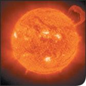
(b) By doing experiments in apparent weightlessness on board the International Space Station, physicists have been able to make sensitive measurements that would be impossible in Earth’s surface gravity.
CAUTION The meaning of “theory” A theory is not just a random thought or an unproven concept. Rather, a theory is an explanation of natural phenomena based on observation and accepted fundamental principles. An example is the well-established theory of biological evolution, which is the result of extensive research and observation by generations of biologists. ❙
To develop a physical theory, a physicist has to ask appropriate questions, design experiments to try to answer the questions, and draw appropriate conclusions from the results. Figure 1.1 shows two important facilities used for physics experiments.
Legend has it that Galileo Galilei (1564–1642) dropped light and heavy objects from the top of the Leaning Tower of Pisa (Fig. 1.1a) to find out whether their rates of fall were different. From examining the results of his experiments (which were actually much more sophisticated than in the legend), he deduced the theory that the acceleration of a freely falling object is independent of its weight.
The development of physical theories such as Galileo’s often takes an indirect path, with blind alleys, wrong guesses, and the discarding of unsuccessful theories in favor of more promising ones. Physics is not simply a collection of facts and principles; it is also the process by which we arrive at general principles that describe how the physical universe behaves.
No theory is ever regarded as the ultimate truth. It’s always possible that new observations will require that a theory be revised or discarded. Note that we can disprove a theory by finding behavior that is inconsistent with it, but we can never prove that a theory is always correct.
Getting back to Galileo, suppose we drop a feather and a cannonball. They certainly do not fall at the same rate. This does not mean that Galileo was wrong; it means that his theory was incomplete. If we drop the feather and the cannonball in a vacuum to eliminate the effects of the air, then they do fall at the same rate. Galileo’s theory has a range of validity: It applies only to objects for which the force exerted by the air (due to air resistance and buoyancy) is much less than the weight. Objects like feathers or parachutes are clearly outside this range.
1.2 SOLVING PHYSICS PROBLEMS
At some point in their studies, almost all physics students find themselves thinking, “I understand the concepts, but I just can’t solve the problems.” But in physics, truly understanding a concept means being able to apply it to a variety of problems. Learning how to solve problems is absolutely essential; you don’t know physics unless you can do physics. How do you learn to solve physics problems? In every chapter of this book you’ll find Problem-Solving Strategies that offer techniques for setting up and solving problems efficiently and accurately. Following each Problem-Solving Strategy are one or more worked Examples that show these techniques in action. (The Problem-Solving Strategies will also steer you away from some incorrect techniques that you may be tempted to use.) You’ll also find additional examples that aren’t associated with a particular ProblemSolving Strategy. In addition, at the end of each chapter you’ll find a Bridging Problem that uses more than one of the key ideas from the chapter. Study these strategies and problems carefully, and work through each example for yourself on a piece of paper. Different techniques are useful for solving different kinds of physics problems, which is why this book offers dozens of Problem-Solving Strategies. No matter what kind of problem you’re dealing with, however, there are certain key steps that you’ll always follow. (These same steps are equally useful for problems in math, engineering, chemistry, and many other fields.) In this book we’ve organized these steps into four stages of solving a problem.
All of the Problem-Solving Strategies and Examples in this book will follow these four steps. (In some cases we’ll combine the first two or three steps.) We encourage you to follow these same steps when you solve problems yourself. You may find it useful to remember the acronym I SEE—short for Identify, Set up, Execute, and Evaluate.
• Use the physical conditions stated in the problem to help you decide which physics concepts are relevant.
• Identify the target variables of the problem—that is, the quantities whose values you’re trying to find, such as the speed at which a projectile hits the ground, the intensity of a sound made by a siren, or the size of an image made by a lens.
• Identify the known quantities, as stated or implied in the problem. This step is essential whether the problem asks for an algebraic expression or a numerical answer.
SET UP the problem:
• Given the concepts, known quantities, and target variables that you found in the IDENTIFY step, choose the equations that you’ll use to solve the problem and decide how you’ll use them. Study the worked examples in this book for tips on how to select the proper equations. If this seems challenging, don’t worry—you’ll get better with practice!
• Make sure that the variables you have identified correlate exactly with those in the equations.
Idealized Models
• If appropriate, draw a sketch of the situation described in the problem. (Graph paper and a ruler will help you make clear, useful sketches.)
EXECUTE the solution:
• Here’s where you’ll “do the math” with the equations that you selected in the SET UP step to solve for the target variables that you found in the IDENTIFY step. Study the worked examples to see what’s involved in this step.
EVALUATE your answer:
• Check your answer from the SOLVE step to see if it’s reasonable. (If you’re calculating how high a thrown baseball goes, an answer of 1.0 mm is unreasonably small and an answer of 100 km is unreasonably large.) If your answer includes an algebraic expression, confirm that it correctly represents what would happen if the variables in it had very large or very small values.
• For future reference, make note of any answer that represents a quantity of particular significance. Ask yourself how you might answer a more general or more difficult version of the problem you have just solved.
In everyday conversation we use the word “model” to mean either a small-scale replica, such as a model railroad, or a person who displays articles of clothing (or the absence thereof). In physics a model is a simplified version of a physical system that would be too complicated to analyze in full detail.
For example, suppose we want to analyze the motion of a thrown baseball ( Fig. 1. 2a). How complicated is this problem? The ball is not a perfect sphere (it has raised seams), and it spins as it moves through the air. Air resistance and wind influence its motion, the ball’s weight varies a little as its altitude changes, and so on. If we try to include all these effects, the analysis gets hopelessly complicated. Instead, we invent a simplified version of the problem. We ignore the size, shape, and rotation of the ball by representing it as a point object, or particle. We ignore air resistance by making the ball move in a vacuum, and we make the weight constant. Now we have a problem that is simple enough to deal with (Fig. 1.2b). We’ll analyze this model in detail in Chapter 3.
We have to overlook quite a few minor effects to make an idealized model, but we must be careful not to neglect too much. If we ignore the effects of gravity completely, then our model predicts that when we throw the ball up, it will go in a straight line and disappear into space. A useful model simplifies a problem enough to make it manageable, yet keeps its essential features.
The validity of the predictions we make using a model is limited by the validity of the model. For example, Galileo’s prediction about falling objects (see Section 1.1) corresponds to an idealized model that does not include the effects of air resistance. This model works fairly well for a dropped cannonball, but not so well for a feather.
Idealized models play a crucial role throughout this book. Watch for them in discussions of physical theories and their applications to specific problems.
1.3 STANDARDS AND UNITS
As we learned in Section 1.1, physics is an experimental science. Experiments require measurements, and we generally use numbers to describe the results of measurements. Any number that is used to describe a physical phenomenon quantitatively is called
Figure 1.2 To simplify the analysis of (a) a baseball in flight, we use (b) an idealized model.
(a) A real baseball in flight
A baseball spins and has a complex shape.
Air resistance and wind exert forces on the ball.
Gravitational force on ball depends on altitude.
Direction of motion
(b) An idealized model of the baseball
Treat the baseball as a point object (particle).
No air resistance.
Gravitational force on ball is constant.
Direction of motion
Figure 1.3 The measurements used to determine (a) the duration of a second and (b) the length of a meter. These measurements are useful for setting standards because they give the same results no matter where they are made.
(a) Measuring the second
Microwave radiation with a frequency of exactly 9,192,631,770 cycles per second ...
Outermost electron
Cesium-133 atom
... causes the outermost electron of a cesium-133 atom to reverse its spin direction.
Cesium-133 atom
An atomic clock uses this phenomenon to tune microwaves to this exact frequency. It then counts 1 second for each 9,192,631,770 cycles.
(b) Measuring the meter
0:00 s 0:01 s
a physical quantity. For example, two physical quantities that describe you are your weight and your height. Some physical quantities are so fundamental that we can define them only by describing how to measure them. Such a definition is called an operational definition. Two examples are measuring a distance by using a ruler and measuring a time interval by using a stopwatch. In other cases we define a physical quantity by describing how to calculate it from other quantities that we can measure. Thus we might define the average speed of a moving object as the distance traveled (measured with a ruler) divided by the time of travel (measured with a stopwatch).
When we measure a quantity, we always compare it with some reference standard. When we say that a basketball hoop is 3.05 meters above the ground, we mean that this distance is 3.05 times as long as a meter stick, which we define to be 1 meter long. Such a standard defines a unit of the quantity. The meter is a unit of distance, and the second is a unit of time. When we use a number to describe a physical quantity, we must always specify the unit that we are using; to describe a distance as simply “3.05” wouldn’t mean anything.
To make accurate, reliable measurements, we need units of measurement that do not change and that can be duplicated by observers in various locations. The system of units used by scientists and engineers around the world is commonly called “the metric system,” but since 1960 it has been known officially as the International System, or SI (the abbreviation for its French name, Système International ). Appendix A gives a list of all SI units as well as definitions of the most fundamental units.
Time
From 1889 until 1967, the unit of time was defined as a certain fraction of the mean solar day, the average time between successive arrivals of the sun at its highest point in the sky. The present standard, adopted in 1967, is much more precise. It is based on an atomic clock, which uses the energy difference between the two lowest energy states of the cesium atom (133Cs). When bombarded by microwaves of precisely the proper frequency, cesium atoms undergo a transition from one of these states to the other. One second (abbreviated s) is defined as the time required for 9,192,631,770 cycles of this microwave radiation ( Fig. 1. 3a).
Length
In 1960 an atomic standard for the meter was also established, using the wavelength of the orange-red light emitted by excited atoms of krypton 186Kr2. From this length standard, the speed of light in vacuum was measured to be 299,792,458 m>s. In November 1983, the length standard was changed again so that the speed of light in vacuum was defined to be precisely 299,792,458 m>s. Hence the new definition of the meter (abbreviated m) is the distance that light travels in vacuum in 1>299,792,458 second (Fig. 1.3b). This modern definition provides a much more precise standard of length than the one based on a wavelength of light.
Mass
Until recently the unit of mass, the kilogram (abbreviated kg), was defined to be the mass of a metal cylinder kept at the International Bureau of Weights and Measures in France ( Fig. 1. 4). This was a very inconvenient standard to use. Since 2018 the value of the kilogram has been based on a fundamental constant of nature called Planck’s constant (symbol h), whose defined value h = 6.62607015 * 10 -34 kg # m2>s is related to those of the kilogram, meter, and second. Given the values of the meter and the second, the masses of objects can be experimentally determined in terms of h. (We’ll explain the meaning of h in Chapter 28.) The gram (which is not a fundamental unit) is 0.001 kilogram. Light source
Light travels exactly 299,792,458 m in 1 s.
Other derived units can be formed from the fundamental units. For example, the units of speed are meters per second, or m>s; these are the units of length (m) divided by the units of time (s).
Unit Prefixes
Once we have defined the fundamental units, it is easy to introduce larger and smaller units for the same physical quantities. In the metric system these other units are related to the fundamental units (or, in the case of mass, to the gram) by multiples of 10 or 1 10 . Thus one kilometer 11 km2 is 1000 meters, and one centimeter 11 cm2 is 1 100 meter. We usually express multiples of 10 or 1 10 in exponential notation: 1000 = 103, 1 1000 = 10 - 3 , and so on. With this notation, 1 km = 103 m and 1 cm = 10 - 2 m
The names of the additional units are derived by adding a prefix to the name of the fundamental unit. For example, the prefix “kilo-,” abbreviated k, always means a unit larger by a factor of 1000; thus
1 kilometer = 1 km = 103 meters = 103 m
1 kilogram = 1 kg = 103 grams = 103 g
1 kilowatt = 1 kW = 103 watts = 103 W
A table in Appendix A lists the standard SI units, with their meanings and abbreviations.
Table 1.1 gives some examples of the use of multiples of 10 and their prefixes with the units of length, mass, and time. Figure 1. 5 (next page) shows how these prefixes are used to describe both large and small distances.
The British System
Finally, we mention the British system of units. These units are used in only the United States and a few other countries, and in most of these they are being replaced by SI units. British units are now officially defined in terms of SI units, as follows:
Length: 1 inch = 2.54 cm (exactly)
Force: 1 pound = 4.448221615260 newtons (exactly)
The newton, abbreviated N, is the SI unit of force. The British unit of time is the second, defined the same way as in SI. In physics, British units are used in mechanics and thermodynamics only; there is no British system of electrical units.
TABLE 1.1 Some Units of Length, Mass, and Time
1 nanometer = 1 nm = 10 - 9 m
(a few times the size of the largest atom)
1 micrometer = 1 mm = 10 - 6 m
(size of some bacteria and other cells)
1 millimeter = 1 mm = 10 - 3 m
(diameter of the point of a ballpoint pen)
1 centimeter = 1 cm = 10 - 2 m
(diameter of your little finger)
1 kilometer = 1 km = 103 m
(distance in a 10 minute walk)
1 microgram = 1 mg = 10 - 6 g = 10 - 9 kg
(mass of a very small dust particle)
1 milligram = 1 mg = 10 - 3 g = 10 - 6 kg
(mass of a grain of salt)
1 gram = 1 g = 10 - 3 kg
(mass of a paper clip)
Figure 1.4 Until 2018 a metal cylinder was used to define the value of the kilogram. (The one shown here, a copy of the one in France, was maintained by the U. S. National Institute of Standards and Technology.) Today the kilogram is defined in terms of one of the fundamental constants of nature.
1 nanosecond = 1 ns = 10 - 9 s
(time for light to travel 0.3 m)
1 microsecond = 1 ms = 10 - 6 s
(time for space station to move 8 mm)
1 millisecond = 1 ms = 10 - 3 s
(time for a car moving at freeway speed to travel 3 cm)
Note: (f) is a scanning tunneling microscope image of atoms on a crystal surface; (g) is an artist’s impression.
Figure 1.6 Many everyday items make use of both SI and British units. An example is this speedometer from a U.S.-built car, which shows the speed in both kilometers per hour (inner scale) and miles per hour (outer scale).
In this book we use SI units for all examples and problems, but we occasionally give approximate equivalents in British units. As you do problems using SI units, you may also wish to convert to the approximate British equivalents if they are more familiar to you ( Fig. 1.6). But you should try to think in SI units as much as you can.
1.4 USING AND CONVERTING UNITS
We use equations to express relationships among physical quantities, represented by algebraic symbols. Each algebraic symbol always denotes both a number and a unit. For example, d might represent a distance of 10 m, t a time of 5 s, and v a speed of 2 m>s.
An equation must always be dimensionally consistent. You can’t add apples and automobiles; two terms may be added or equated only if they have the same units. For example, if an object moving with constant speed v travels a distance d in a time t, these quantities are related by the equation
d = vt
If d is measured in meters, then the product vt must also be expressed in meters. Using the above numbers as an example, we may write
10 m = a 2 m s b (5 s)
Because the unit s in the denominator of m>s cancels, the product has units of meters, as it must. In calculations, units are treated just like algebraic symbols with respect to multiplication and division.
CAUTION Always use units in calculations Make it a habit to always write numbers with the correct units and carry the units through the calculation as in the example above. This provides a very useful check. If at some stage in a calculation you find that an equation or an expression has inconsistent units, you know you have made an error. In this book we’ll always carry units through all calculations, and we strongly urge you to follow this practice when you solve problems. ❙
(g) 10 - 14 m Radius of an atomic nucleus
(f) 10 -10 m Radius of an atom
(e) 10 - 5 m Diameter of a red blood cell
(d) 1 m Human dimensions
(c) 107 m Diameter of the earth
(b) 1011 m Distance to the sun
(a) 10 26 m Limit of the observable universe
Figure 1.5 Some typical lengths in the universe.
PROBLEM-SOLVING
STRATEGY 1. 2 Unit Conversions
IDENTIFY the relevant concepts: In most cases, it’s best to use the fundamental SI units (lengths in meters, masses in kilograms, and times in seconds) in every problem. If you need the answer to be in a different set of units (such as kilometers, grams, or hours), wait until the end of the problem to make the conversion.
SET UP the problem and EXECUTE the solution: Units are multiplied and divided just like ordinary algebraic symbols. This gives us an easy way to convert a quantity from one set of units to another: Express the same physical quantity in two different units and form an equality.
For example, when we say that 1 min = 60 s, we don’t mean that the number 1 is equal to the number 60; rather, we mean that 1 min represents the same physical time interval as 60 s. For this reason, the ratio (1 min)>(60 s) equals 1, as does its reciprocal, (60 s)>(1 min) We may multiply a quantity by either of these factors
EXAMPLE 1.1 Converting speed units
The world land speed record of 763.0 mi>h was set on October 15, 1997, by Andy Green in the jet-engine car Thrust SSC. Express this speed in meters per second.
IDENTIFY, SET UP, and EXECUTE We need to convert the units of a speed from mi>h to m>s We must therefore find unit multipliers that relate (i) miles to meters and (ii) hours to seconds. In Appendix E we find the equalities 1 mi = 1.609 km, 1 km = 1000 m, and 1 h = 3600 s. We set up the conversion as follows, which ensures that all the desired cancellations by division take place:
(which we call unit multipliers) without changing that quantity’s physical meaning. For example, to find the number of seconds in 3 min, we write 3 min = (3 min) a 60 s 1 min b = 180 s
EVALUATE your answer: If you do your unit conversions correctly, unwanted units will cancel, as in the example above. If, instead, you had multiplied 3 min by (1 min)>(60 s), your result would have been the nonsensical 1 20 min2>s. To be sure you convert units properly, include the units at all stages of the calculation.
Finally, check whether your answer is reasonable. For example, the result 3 min = 180 s is reasonable because the second is a smaller unit than the minute, so there are more seconds than minutes in the same time interval.
EXAMPLE 1. 2 Converting volume units
One of the world’s largest cut diamonds is the First Star of Africa (mounted in the British Royal Sceptre and kept in the Tower of London). Its volume is 1.84 cubic inches. What is its volume in cubic centimeters? In cubic meters?
IDENTIFY, SET UP, and EXECUTE Here we are to convert the units of a volume from cubic inches 1in 32 to both cubic centimeters 1cm32 and cubic meters 1m32 Appendix E gives us the equality 1 in = 2 540 cm, from which we obtain 1 in 3 = (2 54 cm)3. We then have
EVALUATE This example shows a useful rule of thumb: A speed expressed in m>s is a bit less than half the value expressed in mi>h, and a bit less than one-third the value expressed in km>h. For example, a normal freeway speed is about 30 m>s = 67 mi>h = 108 km>h, and a typical walking speed is about 1.4 m>s = 3.1 mi>
>h.
KEYCONCEPT To convert units, multiply by an appropriate unit multiplier.
EVALUATE Following the pattern of these conversions, can you show that 1 in . 3 ≈ 16 cm3 and that 1 m3 ≈ 60,000 in .3?
KEYCONCEPT If the units of a quantity are a product of simpler units, such as m3 = m * m * m, use a product of unit multipliers to convert these units.
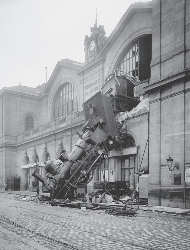
Figure 1.7 This spectacular mishap was the result of a very small percent error— traveling a few meters too far at the end of a journey of hundreds of thousands of meters.
TABLE 1.2 Using Significant Figures
Multiplication or division: Result can have no more significant figures than the factor with the fewest significant figures:
= 0.42
Addition or subtraction:
Number of significant figures is determined by the term with the largest uncertainty (i.e., fewest digits to the right of the decimal point):
1.5 UNCERTAINTY AND SIGNIFICANT FIGURES
Measurements always have uncertainties. If you measure the thickness of the cover of a hardbound version of this book using an ordinary ruler, your measurement is reliable to only the nearest millimeter, and your result will be 3 mm. It would be wrong to state this result as 3.00 mm; given the limitations of the measuring device, you can’t tell whether the actual thickness is 3.00 mm, 2.85 mm, or 3.11 mm. But if you use a micrometer caliper, a device that measures distances reliably to the nearest 0.01 mm, the result will be 2.91 mm. The distinction between the measurements with a ruler and with a caliper is in their uncertainty; the measurement with a caliper has a smaller uncertainty. The uncertainty is also called the error because it indicates the maximum difference there is likely to be between the measured value and the true value. The uncertainty or error of a measured value depends on the measurement technique used.
We often indicate the accuracy of a measured value—that is, how close it is likely to be to the true value—by writing the number, the symbol { , and a second number indicating the uncertainty of the measurement. If the diameter of a steel rod is given as 56.47 { 0.02 mm, this means that the true value is likely to be within the range from 56.45 mm to 56.49 mm. In a commonly used shorthand notation, the number 1.64541212 means 1.6454 { 0.0021 The numbers in parentheses show the uncertainty in the final digits of the main number.
We can also express accuracy in terms of the maximum likely fractional error or percent error (also called fractional uncertainty and percent uncertainty). A resistor labeled ; 47 ohms { 10%< probably has a true resistance that differs from 47 ohms by no more than 10% of 47 ohms—that is, by about 5 ohms. The resistance is probably between 42 and 52 ohms. For the diameter of the steel rod given above, the fractional error is 10.02 mm2>156.47 mm2, or about 0.0004; the percent error is 10.000421100%2, or about 0.04%. Even small percent errors can be very significant ( Fig. 1.7 ).
In many cases the uncertainty of a number is not stated explicitly. Instead, the uncertainty is indicated by the number of meaningful digits, or significant figures, in the measured value. We gave the thickness of the cover of the book as 2.91 mm, which has three significant figures. By this we mean that the first two digits are known to be correct, while the third digit is uncertain. The last digit is in the hundredths place, so the uncertainty is about 0.01 mm. Two values with the same number of significant figures may have different uncertainties; a distance given as 137 km also has three significant figures, but the uncertainty is about 1 km. A distance given as 0.25 km has two significant figures (the zero to the left of the decimal point doesn’t count); if given as 0.250 km, it has three significant figures.
Figure 1.8 Determining the value of p from the circumference and diameter of a circle.
When you use numbers that have uncertainties to compute other numbers, the computed numbers are also uncertain. When numbers are multiplied or divided, the result can have no more significant figures than the factor with the fewest significant figures has. For example, 3.1416 * 2.34 * 0.58 = 4.3. When we add and subtract numbers, it’s the location of the decimal point that matters, not the number of significant figures. For example, 123.62 + 8.9 = 132.5 Although 123.62 has an uncertainty of about 0.01, 8.9 has an uncertainty of about 0.1. So their sum has an uncertainty of about 0.1 and should be written as 132.5, not 132.52. Table 1. 2 summarizes these rules for significant figures.
To apply these ideas, suppose you want to verify the value of p, the ratio of the circumference of a circle to its diameter. The true value of this ratio to ten digits is 3.141592654. To test this, you draw a large circle and measure its circumference and diameter to the nearest millimeter, obtaining the values 424 mm and 135 mm ( Fig. 1. 8). You enter these into your calculator and obtain the quotient 1424 mm2>1135 mm2 = 3.140740741. This may seem to disagree with the true value of p, but keep in mind that each of your measurements has three significant figures, so your measured value of p can have only three significant figures. It should be stated simply as 3.14. Within the limit of three significant figures, your value does agree with the true value.
424 mm
The measured values have only three significant figures, so their calculated ratio (p) also has only three significant figures.
In the examples and problems in this book we usually give numerical values with three significant figures, so your answers should usually have no more than three significant figures. (Many numbers in the real world have even less accuracy. The speedometer in a car, for example, usually gives only two significant figures.) Even if you do the arithmetic with a
calculator that displays ten digits, a ten-digit answer would misrepresent the accuracy of the results. Always round your final answer to keep only the correct number of significant figures or, in doubtful cases, one more at most. In Example 1.1 it would have been wrong to state the answer as 341.01861 m>s Note that when you reduce such an answer to the appropriate number of significant figures, you must round, not truncate. Your calculator will tell you that the ratio of 525 m to 311 m is 1.688102894; to three significant figures, this is 1.69, not 1.68.
Here’s a special note about calculations that involve multiple steps: As you work, it’s helpful to keep extra significant figures in your calculations. Once you have your final answer, round it to the correct number of significant figures. This will give you the most accurate results.
When we work with very large or very small numbers, we can show significant figures much more easily by using scientific notation, sometimes called powers-of-10 notation. The distance from the earth to the moon is about 384,000,000 m, but writing the number in this form doesn’t indicate the number of significant figures. Instead, we move the decimal point eight places to the left (corresponding to dividing by 108) and multiply by 108; that is,
384,000,000 m = 3.84 * 108 m
In this form, it is clear that we have three significant figures. The number 4.00 * 10 - 7 also has three significant figures, even though two of them are zeros. Note that in scientific notation the usual practice is to express the quantity as a number between 1 and 10 multiplied by the appropriate power of 10.
When an integer or a fraction occurs in an algebraic equation, we treat that number as having no uncertainty at all. For example, in the equation vx 2 = v0x 2 + 2ax 1x - x02, which is Eq. (2.13) in Chapter 2, the coefficient 2 is exactly 2. We can consider this coefficient as having an infinite number of significant figures (2.000000 c). The same is true of the exponent 2 in vx 2 and v0x 2 .
Finally, let’s note that precision is not the same as accuracy. A cheap digital watch that gives the time as 10:35:17 a.m. is very precise (the time is given to the second), but if the watch runs several minutes slow, then this value isn’t very accurate. On the other hand, a grandfather clock might be very accurate (that is, display the correct time), but if the clock has no second hand, it isn’t very precise. A high-quality measurement is both precise and accurate.
EXAMPLE 1. 3 Significant figures in multiplication
The rest energy E of an object with rest mass m is given by Albert Einstein’s famous equation E = mc2, where c is the speed of light in vacuum. Find E for an electron for which (to three significant figures) m = 9.11 * 10 - 31 kg. The SI unit for E is the joule (J); 1 J = 1 kg # m2>s2.
IDENTIFY and SET UP Our target variable is the energy E. We are given the value of the mass m; from Section 1.3 (or Appendix F) the speed of light is c = 2.99792458 * 108 m>s.
EXECUTE Substituting the values of m and c into Einstein’s equation, we find
E = 19 11 * 10 - 31 kg212 99792458 * 108 m>s22
= 19 11212 9979245822110 - 312110822 kg # m2>s2
= 181 876596782110 3 - 31 + 12 * 8242 kg # m2>s2
= 8.187659678 * 10 - 14 kg # m2>s2
Since the value of m was given to only three significant figures, we must round this to E = 8 19 * 10 - 14 kg # m2>s2 = 8 19 * 10 - 14 J
EVALUATE While the rest energy contained in an electron may seem ridiculously small, on the atomic scale it is tremendous. Compare our answer to 10 - 19 J, the energy gained or lost by a single atom during a typical chemical reaction. The rest energy of an electron is about 1,000,000 times larger! (We’ll discuss the significance of rest energy in Chapter 37.)
KEYCONCEPT When you are multiplying (or dividing) quantities, the result can have no more significant figures than the quantity with the fewest significant figures.
TEST YOUR UNDERSTANDING OF SECTION 1. 5 The density of a material is equal to its mass divided by its volume. What is the density 1in kg>m32 of a rock of mass 1.80 kg and volume 6 0 * 10 - 4 m3? (i) 3 * 103 kg>m3; (ii) 3 0 * 103 kg >m3; (iii) 3 00 * 103 kg>m3; (iv) 3 000 * 103 kg>m3; (v) any of these—all of these answers are mathematically equivalent.
ANSWER
number with the fewest significant figures controls the number of significant figures in the result.
❙ (ii) ytisneD = 11 08 gk1>26 0 * 01 - 4 3m2 = 3 0 * 301 gk>3m When we multiply or divide, the
1.6 ESTIMATES AND ORDERS OF MAGNITUDE
We have stressed the importance of knowing the accuracy of numbers that represent physical quantities. But even a very crude estimate of a quantity often gives us useful information. Sometimes we know how to calculate a certain quantity, but we have to guess at the data we need for the calculation. Or the calculation might be too complicated to carry out exactly, so we make rough approximations. In either case our result is also a guess, but such a guess can be useful even if it is uncertain by a factor of two, ten, or more. Such calculations are called order-of-magnitude estimates. The great Italian-American nuclear physicist Enrico Fermi (1901–1954) called them “back-of-the-envelope calculations.”
Exercises 1.15 through 1.20 at the end of this chapter are of the estimating, or order-ofmagnitude, variety. Most require guesswork for the needed input data. Don’t try to look up a lot of data; make the best guesses you can. Even when they are off by a factor of ten, the results can be useful and interesting.
EXAMPLE 1. 4 An order-of-magnitude estimate
You are writing an adventure novel in which the hero escapes with a billion dollars’ worth of gold in his suitcase. Could anyone carry that much gold? Would it fit in a suitcase?
IDENTIFY, SET UP, and EXECUTE Gold sells for about $1400 an ounce, or about $100 for 1 14 ounce. (The price per ounce has varied between $200 and $1900 over the past twenty years or so.) An ounce is about 30 grams, so $100 worth of gold has a mass of about 1 14 of 30 grams, or roughly 2 grams. A billion 11092 dollars’ worth of gold has a mass 107 times greater, about 2 * 107 120 million2 grams or 2 * 104 120,0002 kilograms. A thousand kilograms has a weight in British units of about a ton, so the suitcase weighs roughly 20 tons! No human could lift it.
Roughly what is the volume of this gold? The density of water is 103 kg>m3; if gold, which is much denser than water, has a density 10 times greater, then 104 kg of gold fits into a volume of 1 m3. So 109 dollars’ worth of gold has a volume of 2 m 3, many times the volume of a suitcase.
EVALUATE Clearly your novel needs rewriting. Try the calculation again with a suitcase full of five-carat (1-gram) diamonds, each worth $500,000. Would this work?
KEYCONCEPT To decide whether the numerical value of a quantity is reasonable, assess the quantity in terms of other quantities that you can estimate, even if only roughly.
TEST YOUR UNDERSTANDING OF SECTION 1.6 Can you estimate the total number of teeth in the mouths of all the students on your campus? (Hint: How many teeth are in your mouth? Count them!)
ANSWER
APPLICATION Scalar
Temperature, Vector Wind The comfort level on a wintry day depends on the temperature, a scalar quantity that can be positive or negative (say, + 5°C or - 20°C) but has no direction. It also depends on the wind velocity, a vector quantity with both magnitude and direction (for example, 15 km>h from the west).
1.7 VECTORS AND VECTOR ADDITION
Some physical quantities, such as time, temperature, mass, and density, can be described completely by a single number with a unit. But many other important quantities in physics have a direction associated with them and cannot be described by a single number. A simple example is the motion of an airplane: We must say not only how fast the plane is moving but also in what direction. The speed of the airplane combined with its direction of motion constitute a quantity called velocity. Another example is force, which in physics means a push or pull exerted on an object. Giving a complete description of a force means describing both how hard the force pushes or pulls on the object and the direction of the push or pull.
When a physical quantity is described by a single number, we call it a scalar quantity. In contrast, a vector quantity has both a magnitude (the “how much” or “how big” part) and a direction in space. Calculations that combine scalar quantities use the operations of ordinary arithmetic. For example, 6 kg + 3 kg = 9 kg, or 4 * 2 s = 8 s. However, combining vectors requires a different set of operations.
To understand more about vectors and how they combine, we start with the simplest vector quantity, displacement. Displacement is a change in the position of an object. ❙ The answer depends on how many students are enrolled at your campus.
Displacement is a vector quantity because we must state not only how far the object moves but also in what direction. Walking 3 km north from your front door doesn’t get you to the same place as walking 3 km southeast; these two displacements have the same magnitude but different directions.
We usually represent a vector quantity such as displacement by a single letter, such as A S in Fig. 1.9a. In this book we always print vector symbols in boldface italic type with an arrow above them. We do this to remind you that vector quantities have different properties from scalar quantities; the arrow is a reminder that vectors have direction. When you handwrite a symbol for a vector, always write it with an arrow on top. If you don’t distinguish between scalar and vector quantities in your notation, you probably won’t make the distinction in your thinking either, and confusion will result.
We always draw a vector as a line with an arrowhead at its tip. The length of the line shows the vector’s magnitude, and the direction of the arrowhead shows the vector’s direction. Displacement is always a straight-line segment directed from the starting point to the ending point, even though the object’s actual path may be curved (Fig. 1.9b). Note that displacement is not related directly to the total distance traveled. If the object were to continue past P2 and then return to P1 , the displacement for the entire trip would be zero (Fig. 1.9c).
If two vectors have the same direction, they are parallel. If they have the same magnitude and the same direction, they are equal, no matter where they are located in space. The vector A S ′ from point P3 to point P4 in Fig. 1.10 has the same length and direction as the vector A S from P1 to P2 . These two displacements are equal, even though they start at different points. We write this as A S ′ = A S in Fig. 1.10; the boldface equals sign emphasizes that equality of two vector quantities is not the same relationship as equality of two scalar quantities. Two vector quantities are equal only when they have the same magnitude and the same direction.
Vector B S in Fig. 1.10, however, is not equal to A S because its direction is opposite that of A S . We define the negative of a vector as a vector having the same magnitude as the original vector but the opposite direction. The negative of vector quantity A S is denoted as A S , and we use a boldface minus sign to emphasize the vector nature of the quantities. If A S is 87 m south, then A S is 87 m north. Thus we can write the relationship between A S and B S in Fig. 1.10 as A S = B S or B S = A S . When two vectors A S and B S have opposite directions, whether their magnitudes are the same or not, we say that they are antiparallel.
We usually represent the magnitude of a vector quantity by the same letter used for the vector, but in lightface italic type with no arrow on top. For example, if displacement vector A S is 87 m south, then A = 87 m. An alternative notation is the vector symbol with vertical bars on both sides:
1Magnitude of A S 2 = A = A S ( 1.1)
The magnitude of a vector quantity is a scalar quantity (a number) and is always positive. Note that a vector can never be equal to a scalar because they are different kinds of quantities. The expression ; A S = 6 m< is just as wrong as ; 2 oranges = 3 apples<! When we draw diagrams with vectors, it’s best to use a scale similar to those used for maps. For example, a displacement of 5 km might be represented in a diagram by a vector 1 cm long, and a displacement of 10 km by a vector 2 cm long.
Vector Addition and Subtraction
Suppose a particle undergoes a displacement A S followed by a second displacement B S . The final result is the same as if the particle had started at the same initial point and undergone a single displacement C S ( Fig. 1.11a, next page). We call displacement C S the vector sum, or resultant, of displacements A S and B S . We express this relationship symbolically as
C S = A S + B S ( 1.2)
The boldface plus sign emphasizes that adding two vector quantities requires a geometrical process and is not the same operation as adding two scalar quantities such as 2 + 3 = 5 In vector addition we usually place the tail of the second vector at the head, or tip, of the first vector (Fig. 1.11a).
Figure 1.9 Displacement as a vector quantity.
(a) We represent a displacement by an arrow that points in the direction of displacement.
Ending position: P2
Displacement A
Starting position: P1
Handwritten notation:
(b) A displacement is always a straight arrow directed from the starting position to the ending position. It does not depend on the path taken, even if the path is curved.
Path taken
(c) Total displacement for a round trip is 0, regardless of the path taken or distance traveled.
Figure 1.10 The meaning of vectors that have the same magnitude and the same or opposite direction.
Displacements A and A′ are equal because they have the same length and direction.
Displacement B has the same magnitude as A but opposite direction; B is the negative of A
Figure 1.11 Three ways to add two vectors.
(a) We can add two vectors by placing them head to tail.
The vector sum C extends from the tail of vector A S S ... to the head of vector B S
If we make the displacements A S and B S in reverse order, with B S first and A S second, the result is the same (Fig. 1.11b). Thus
C S = B S + A S and A S + B S = B S + A S ( 1.3)
This shows that the order of terms in a vector sum doesn’t matter. In other words, vector addition obeys the commutative law.
S S S S
(b) Adding them in reverse order gives the same result: A + B = B + A. The order doesn’t matter in vector addition.
C = B + A S S
S S S S
= A + B S S S C = A + B S S
Figure 1.11c shows another way to represent the vector sum: If we draw vectors A S and B S with their tails at the same point, vector C S is the diagonal of a parallelogram constructed with A S and B S as two adjacent sides.
CAUTION Magnitudes in vector addition It’s a common error to conclude that if C S = A S + B S , then magnitude C equals magnitude A plus magnitude B. In general, this conclusion is wrong; for the vectors shown in Fig. 1.11, C 6 A + B The magnitude of A S + B S depends on the magnitudes of A S and B S and on the angle between A S and B S . Only in the special case in which A S and B S are parallel is the magnitude of C S = A S + B S equal to the sum of the magnitudes of A S and B S ( Fig. 1.12a). When the vectors are antiparallel (Fig. 1.12b), the magnitude of C S equals the difference of the magnitudes of A S and B S Be careful to distinguish between scalar and vector quantities, and you’ll avoid making errors about the magnitude of a vector sum. ❙
(c) We can also add two vectors by placing them tail to tail and constructing a parallelogram.
Figure 1.12 Adding vectors that are (a) parallel and (b) antiparallel.
(a) Only when vectors A and B are parallel does the magnitude of their vector sum C equal the sum of their magnitudes: C = A + B S S S
S S S
(b) When A and B are antiparallel, the magnitude of their vector sum C equals the difference of their magnitudes: C = A - B .
Figure 1.13a shows three vectors A S , B S , and C S . To find the vector sum of all three, in Fig. 1.13b we first add A S and B S to give a vector sum D S ; we then add vectors C S and D S by the same process to obtain the vector sum R S :
R S = 1A S + B S 2 + C S = D S + C S
Alternatively, we can first add B S and C S to obtain vector E S (Fig. 1.13c), and then add A S and E S to obtain R S :
R S = A S + 1B S + C S 2 = A S + E S
We don’t even need to draw vectors D S and E S ; all we need to do is draw A S , B S , and C S in succession, with the tail of each at the head of the one preceding it. The sum vector R S extends from the tail of the first vector to the head of the last vector (Fig. 1.13d). The order makes no difference; Fig. 1.13e shows a different order, and you should try others. Vector addition obeys the associative law.
We can subtract vectors as well as add them. To see how, recall that vector − A S has the same magnitude as A S but the opposite direction. We define the difference A S B S of two vectors A S and B S to be the vector sum of A S and B S :
S − B S = A S + 1 − B S 2 ( 1.4)
Figure 1.14 shows an example of vector subtraction.
Figure 1.13 Several constructions for finding the vector sum A S + B S + C S
(a) To find the sum of these three vectors ...
S
S S S S S
S S S S S S (c) ... or add B and C to get E and then add E to A to get R ...
S S S S (d) ... or add A, B, and C to get R directly ...
S S S S (e) ... or add A, B, and C in any other order and still get R. (b) ... add A and B to get D and then add C to D to get the final sum (resultant) R