Thermodynamic Models for Chemical Processes
Design, Develop, Analyze and Optimize
Jean-Noël Jaubert Romain Privat
First published 2020 in Great Britain and the United States by ISTE Press Ltd and Elsevier Ltd
Apart from any fair dealing for the purposes of research or private study, or criticism or review, as permitted under the Copyright, Designs and Patents Act 1988, this publication may only be reproduced, stored or transmitted, in any form or by any means, with the prior permission in writing of the publishers, or in the case of reprographic reproduction in accordance with the terms and licenses issued by the CLA. Enquiries concerning reproduction outside these terms should be sent to the publishers at the undermentioned address:
ISTE Press Ltd
27-37 St George’s Road
Elsevier Ltd
The Boulevard, Langford Lane London SW19 4EU Kidlington, Oxford, OX5 1GB UK UK
www.iste.co.uk
www.elsevier.com
Notices
Knowledge and best practice in this field are constantly changing. As new research and experience broaden our understanding, changes in research methods, professional practices, or medical treatment may become necessary.
Practitioners and researchers must always rely on their own experience and knowledge in evaluating and using any information, methods, compounds, or experiments described herein. In using such information or methods they should be mindful of their own safety and the safety of others, including parties for whom they have a professional responsibility.
To the fullest extent of the law, neither the Publisher nor the authors, contributors, or editors, assume any liability for any injury and/or damage to persons or property as a matter of products liability, negligence or otherwise, or from any use or operation of any methods, products, instructions, or ideas contained in the material herein.
For information on all our publications visit our website at http://store.elsevier.com/
© ISTE Press Ltd 2021
The rights of Jean-Noël Jaubert and Romain Privat to be identified as the authors of this work have been asserted by them in accordance with the Copyright, Designs and Patents Act 1988.
British Library Cataloguing-in-Publication Data
A CIP record for this book is available from the British Library Library of Congress Cataloging in Publication Data
A catalog record for this book is available from the Library of Congress
ISBN 978-1-78548-209-0
Printed and bound in the UK and US
1.2. Thermodynamics of the vapor–liquid equilibrium of a pure substance: what should be remembered .................. 2
1.2.1. Phase-intensive variables and global-intensive variables ...... 2
1.2.2. Conditions of two-phase equilibrium of a pure substance ...... 5
1.2.3. Why should the intensive properties of the liquid and vapor phases of a pure substance in vapor–liquid equilibrium be seen as temperature functions? .............................. 5
1.2.4. Critical point of a pure substance .................... 9
1.2.5. Isotherms of a pure species in the fluid region ............. 9
1.2.6. Property changes on vaporization .................... 11
1.3. Correlations for the saturated vapor pressure of pure substances .... 12
1.3.1. Practical expressions for the saturated vapor pressure deduced from the Clapeyron equation ..................... 12
1.3.2. Empirical expressions (Antoine, Wagner, Frost–Kalkwarf) ..... 17
1.3.3. Taking things further: constraints on the curvature of the graphical representation of ln Psat versus 1/T ............... 17
1.3.4. Focus on the Antoine equation ...................... 20
1.4. Equations that can be used to correlate the molar volumes of pure liquids ......................... 22
1.4.1. Correlations that can be used for molar volumes of saturated liquids ....................... 22
1.4.2. Correlations that can be used for molar volumes of subcooled liquids
1.5. Equations that can be used to correlate the molar volumes of saturated gases
1.6. Equations that can be used to correlate the enthalpies of vaporization
1.6.1. Use of the Clapeyron equation
1.6.2. Expression involving many adjustable parameters
1.7. Equations used to correlate the heat capacity at constant molar pressure, molar enthalpy or molar entropy of an incompressible liquid
1.8. Equations that can be used to correlate the molar heat capacity at constant pressure, molar enthalpy or molar entropy of a perfect gas
1.9. Density of a pure substance
1.10. Prediction of the thermodynamic properties of pure substances
2.1.
Presentation of usual volumetric
2.3.1.
2.3.3.
2.3.4.
2.3.5.
2.4.
2.4.1.
2.5.
2.5.1.
2.5.2.
2.5.3. Calculation of state-property
2.6. Vapor–liquid equilibrium calculation using a pressure-explicit equation of state:
2.6.1. Shapes of isotherms produced by cubic equations of state in the pressure–molar volume plane: link between the form of isotherms and the resolution of cubic equations of state ...........
2.6.2. Stable, metastable, unstable roots ....................
2.6.3. Graphical determination of the saturated vapor pressure by the Maxwell equal area rule ..........................
2.6.4. Plot of the stable portions of an isotherm from an equation of state .............................
2.6.5. Calculation of the vaporization properties using an equation of state .............................
2.7. Overall summary: criteria for selecting an equation of state for modeling of the thermodynamic properties of a given pure fluid .......
Chapter 3. Low-Pressure Vapor–Liquid and Liquid–Liquid Equilibria of Binary Systems: Activity-Coefficient Models
3.1. Introduction ....................................
3.2. Classification of fluid-phase behaviors of binary systems at low pressure and low temperature ..................
3.2.1. Conventions for representation of isobaric and isothermal phase diagrams of binary systems .................
3.2.2. The four types of vapor–liquid equilibrium (VLE) diagrams for low temperature, low pressure ..................
3.2.3. Five types of liquid–liquid equilibrium (LLE) diagrams ....... 86
3.2.4. Fluid-phase diagrams resulting from the overlap of LLE and VLE domains. Liquid–liquid–vapor equilibria (VLLE) .............. 92
3.3. Condition of equilibrium between fluid phases of binary systems ... 100
3.4. Vapor–liquid equilibrium relationship at low pressure .......... 101
3.4.1. Estimation of the fugacity coefficient of a pure substance, present in the expression of function Ci ..................... 103
3.4.2. Estimation of the fugacity coefficient of a component in a mixture, present in the expression of function Ci ............... 104
3.4.3. Estimation of the Poynting factor, present in the expression of the function Ci .................................. 105
3.4.4. Estimation of the Ci term .........................
3.5. Activity coefficients: definition and models ................
3.5.1. Ideal solution ................................
3.5.2. Excess Gibbs energy and activity coefficients .............
3.5.3. Classification of activity-coefficient models ..............
3.5.4. Purely correlative Margules models ...................
3.5.5. Redlich–Kister purely correlative model ................
3.5.6. The Van Laar model ............................
3.5.7. The Scatchard–Hildebrand (SH) model .................
3.5.8. The NRTL (non-random two-liquid) model with three adjustable parameters per binary system ...........................
3.5.9. NRTL models with four and six adjustable parameters per binary system ...........................
3.5.10. Wilson and Flory–Huggins models
3.5.11. UNIQUAC model
3.5.12. The original UNIFAC model and its extensions
3.5.13. Summary: an aid to selecting an activity-coefficient model
3.6. Calculation of the vapor–liquid equilibrium of binary systems at low temperature and low pressure
3.6.1. Bubble-point pressure calculation
3.6.2. Calculation of the dew-point pressure
3.6.3. Calculation of the bubble-point temperature
3.6.4. Calculation of the dew-point temperature
3.6.5. PT-flash calculation
Chapter 4. Estimation of the Thermodynamic Properties of Mixtures
4.1. The phase-equilibrium condition and the ϕ-ϕ approach..........
4.2. General presentation of the usual volumetric equations of state
4.3.
4.4. Cubic equations of state
4.4.1. Generalities .................................
4.4.2. Classic mixing rules (known as “Van der Waals” mixing rules) ..
4.4.3. Advanced mixing rules by combining an equation of state with an activity-coefficient model ..................... 147
4.4.4. Short summary of the mixing rules for cubic equations of state ..............................
4.5. Equations of state based on the “statistical associating fluid theory” (SAFT) ......................................... 158
4.6. Specific equations of state for particular mixtures ............. 161
4.7. Practical use of the equations of state for mixtures ............ 161
4.7.1. What can be calculated from an equation of state for mixtures? .......................... 161
4.7.2. Calculation of mixing properties using a pressure-explicit equation of state ........................ 162
4.7.3. Calculation principle of vapor–liquid equilibrium using the ϕ-ϕ approach .............................. 165
Chapter
General
5.1. Selection of thermodynamic models for representation of pure substances
5.2. Selection of thermodynamic models for representation of mixtures
This page intentionally left blank
Preface
This book is not a course book but a vademecum aimed primarily at users of process simulation software. It provides, in a condensed form, the methods governing the choice of a thermodynamic model for a targeted application and reminds the reader of the essential concepts on which these methods are based. At the time of publication (2020), this book was up to date with the main models of practical interest for the engineer and the researcher.
Finally, because we are convinced that, in order to use these models properly, it is important to understand – at the very least – how to carry out the calculations of the properties of interest that result from them, we will also refer to the major points.
Happy reading!
Jean-Noël JAUBERT Romain PRIVAT
May 2020
Correlations for the Estimation of Thermodynamic Properties of Pure Substances in the Liquid, Perfect Gas or Vapor–Liquid States
1.1. Introduction
A correlation is a mathematical expression, usually simple, of a physico-chemical property y as a function of one or several variables x. In this chapter, dedicated to pure substances, two types of properties are considered:
– properties depending on the temperature: for example, the heat capacity at constant pressure of a liquid pure substance (assumed to be incompressible), the saturated vapor pressure of a pure substance, the density of a liquid pure substance (assumed to be incompressible), etc. In these cases, the variable of the correlations is x = T;
– constant properties (which do not depend on the temperature): for example, the normal boiling point, the critical pressure, the acentric factor, etc.
We will look at which principal correlations can be used for the pure-substance thermodynamic properties that depend on the temperature T . This chapter will end with a brief presentation of the methods that allow us to predict the constant properties and those depending on T using only knowledge of the chemical structure of pure substances. The variables x of correlations then become structural information (as well as T in the case of properties that depend on the temperature).
The T-dependent properties that are taken into consideration in this chapter are:
– the characteristic properties of the vapor–liquid equilibrium of a pure substance: saturated vapor pressure ()PsatT , molar enthalpies of a boiling liquid () sat L hT and of saturated vapor () sat G hT , molar enthalpy of vaporization ()()() =− satsat vapGLHThThT Δ , molar heat capacity at constant pressure of the boiling liquid , () sat PL cT , densities of the boiling liquid () sat LTρ or of the saturated gas () sat GTρ ;
– properties of a pure perfect gas: molar enthalpy () • hT , molar heat capacity at constant pressure () • P cT ;
– properties of a subcooled liquid1: molar enthalpy () pure L hT , molar heat capacity at constant pressure , () pure PL cT , volumetric mass () pure LTρ . Here, we assume that pure subcooled liquids are incompressible; in other words, their properties are not affected by the pressure.
NOTE.– Properties of a non-perfect gaseous pure substance cannot be described by the correlations presented in this chapter. Suitable methods (mainly based on equations of state) are presented in the following chapters.
1.2. Thermodynamics of the vapor–liquid equilibrium of a pure substance: what should be remembered
1.2.1. Phase-intensive variables and global-intensive variables
The intensive state of a two-phase system can be described by two sets of variables:
– phase-intensive variables, which are the intensive variables specific to one of the two phases of the system, for example, the temperature of the liquid phase, the pressure of the gas phase, the density of the liquid, the molar heat capacity of the gas phase at constant pressure, etc.;
1 The term “subcooled” refers to a liquid that has been brought to a temperature below its boiling point. Consequently, the pure substance is not boiling (is not at vapor–liquid equilibrium).
– global-intensive variables that are not specific to a given phase but which instead characterize the two-phase system as a whole (i.e. the whole system). As an example, we cite the molarproportionofthegas phase (defined as the quantity of matter present in the gas phase divided by the global quantity of matter in the system, i.e. the sum of the quantities of matter in the liquid and gas phases), the global density (defined as the global mass of the system, i.e. , liquidgasmm + divided by the global volume, i.e. + liquidgasVV ), etc.
NOTE.– As explained in the following, at the vapor–liquid equilibrium, the two phases have the same temperature (), = LGTT the same pressure () = LGPP and each component has the same chemical potential in each phase ,, (). μμ = iLiG Thus, the temperature, pressure and chemical potential of a component i are both phase-intensive and global-intensive variables.
Since the extensive properties are additive, the global extensive properties of a two-phase system are obtained by adding the extensive properties of the two phases:
two-phaseliquid phasegas phase system
Extensive propertyExtensive property of the liquid phaseof the gas phase Global extensive property
(quantity of matter in mol) (volu
1 me in m) (enthalpy in J) (heat capacity in JK)
Consequently, the relationship between the molar properties of the phases that derive from extensive properties ( liquid phase liquid phase gas phase liquid phase , Q qq n ==
phase gas phase Q n ) and global molar properties ( two-phase system two-phase system two-phase system Q q n = ) is:
with { } ,,.... Pqvhc = Equation [1.2] introduces the molar proportions of the phases:
Molar proportion of gas: /
Molar proportion of liquid:1 / =
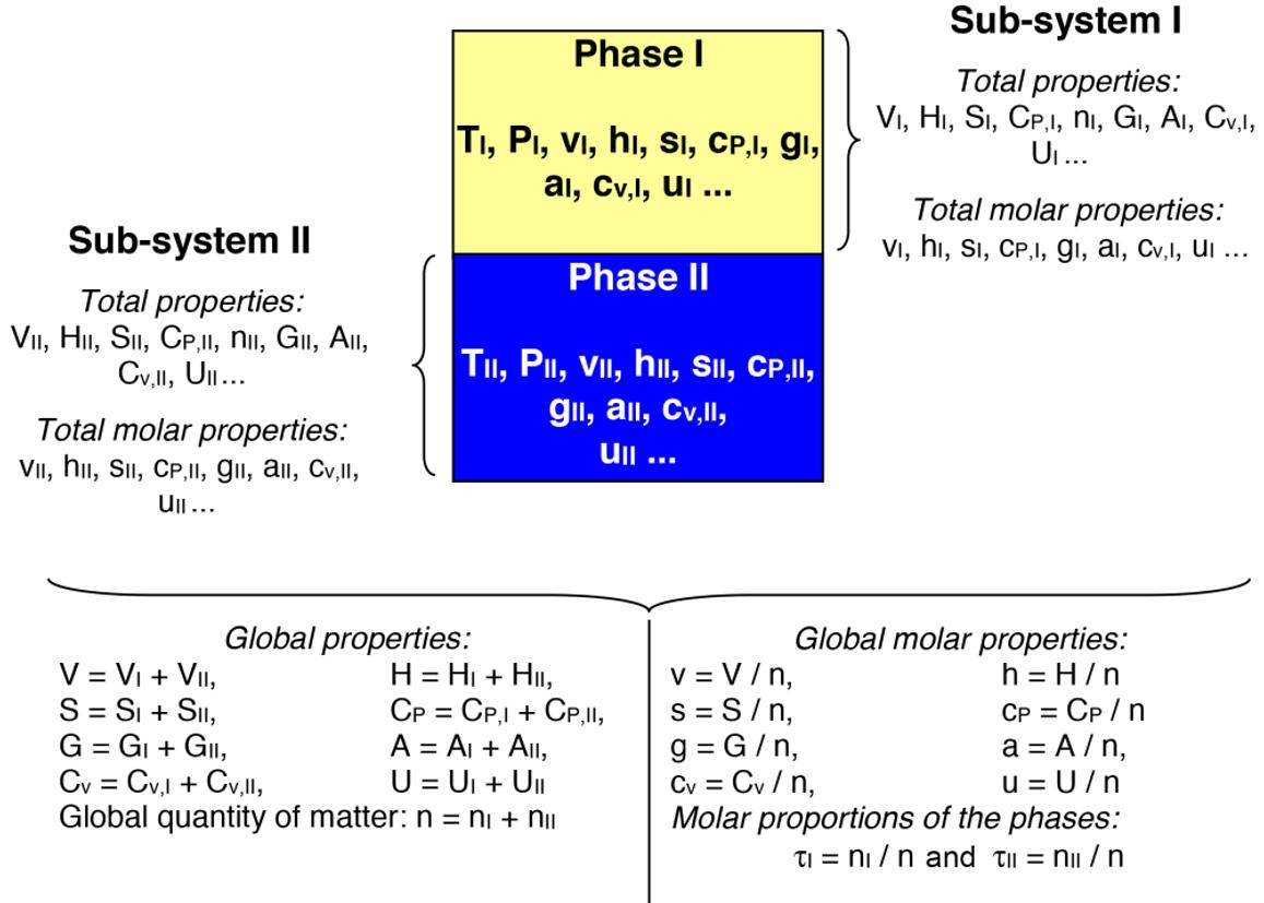
Figure 1.1 represents a two-phase system that illustrates, on the one hand, the notion of extensive (also known as total) and intensive properties that are specific to one of the phases, and, on the other hand, the notion of properties that are characteristic of the two-phase system (known as global).
Figure 1.1. Definition of total, total molar, global and global molar properties
1.2.2. Conditions of two-phase equilibrium of a pure substance
For two-phase equilibrium to be observed, three conditions must be met:
– thermal equilibrium condition: there is no heat transfer between the phases in equilibrium, and consequently, these necessarily have the same temperature: = IIITT [1.4]
– mechanical condition of equilibrium: there is no work transfer of the pressure forces between the phases in equilibrium, and consequently, these are necessarily at the same pressure:
= IIIPP [1.5]
– diffusive equilibrium condition: there is no transfer of matter between the phases in equilibrium, and consequently, the chemical potential of the pure substance g (molar Gibbs energy) is the same in both phases: = gIII g [1.6]
1.2.3. Why should the intensive properties of the liquid and vapor phases of a pure substance in vapor–liquid equilibrium be seen as temperature functions?
The answer to this question is provided by the Gibbs phase rule described below. This theorem concerns the variance of a thermodynamic system, the definition of which is also provided.
According to the previous paragraph, the intensive variables of a phase α are the temperature , Tα the pressure Pα and the total molar properties yα { } (,,,...). yvhgs ∈
DEFINITION.– The variance is defined as the number of independent INTENSIVE variables of PHASES that need to be set (specified) in order to characterize the INTENSIVE variables of ALL PHASES.
The Gibbs phase rule is a theorem asserting that the variance of a thermodynamic system that contains one or several phases in equilibrium, with no other characteristics, is given by the expression:
variance of the system
2with:c = number of components number of phases in equilibrium
Consequently, the variance of a two-phase system ( 2 = ϕ ) that contains a pure substance ( 1 = c ) is 1. υ = This means that by specifying a single intensive variable of one out of the two phases, and the value of all the others is then set.
For example, let us suppose that the pressure GP of the gas phase of a pure substance in vapor–liquid equilibrium is specified. Because of the Gibbs phase rule, this then necessarily sets the pressure of the other phase in equilibrium (this is obvious as the condition of equilibrium between phases imposes = LGPP ), the temperature common to the two phases = LGTT (common according to the phase-equilibrium condition), the molar volumes sat Lv and sat Gv of the phases, the molar enthalpies sat Lh and sat Gh of the phases, etc.
A two-phase equilibrium is therefore monovariant. This feature induces an immediate graphical consequence: in the plane projections of phase diagrams for pure substances with two intensive phase variables as X and Y coordinates (e.g. pressure–molar volume, pressure–temperature, molar enthalpy–molar entropy planes), two-phase equilibria are represented by curves (the curves are the graphical representations of single-variable functions).
Similarly, the Gibbs phase rule, which predicts that the variance of a pure single-phase substance ( 1 = ϕ ) is equal to 2 and that the variance for a pure three-phase substance is zero, the associated graphical representations in the plane projections of the phase diagrams will be surface regions and single points respectively. These remarks are summarized in Figure 1.2 (the definition of the critical point, which is represented in this figure, will be provided at a later stage).
Melting curve
Single-phase solid ν = 2
= 1
= 1
Sublimation curve
= 1
Single-phase liquid ν = 2 Triple point (LSVE)
= 0
point
= 0
Vaporization curve
Single-phase vapor
= 2
Figure 1.2. Projection of the phase diagram for a pure substance in the pressure–temperature plane. Illustration of the relationship between the variance of a system and the nature of its representation on the plane. VLE = vapor–liquid equilibrium, LSE = liquid–solid equilibrium, SVE = solid–vapor equilibrium, LSVE = liquid–solid–vapor equilibrium
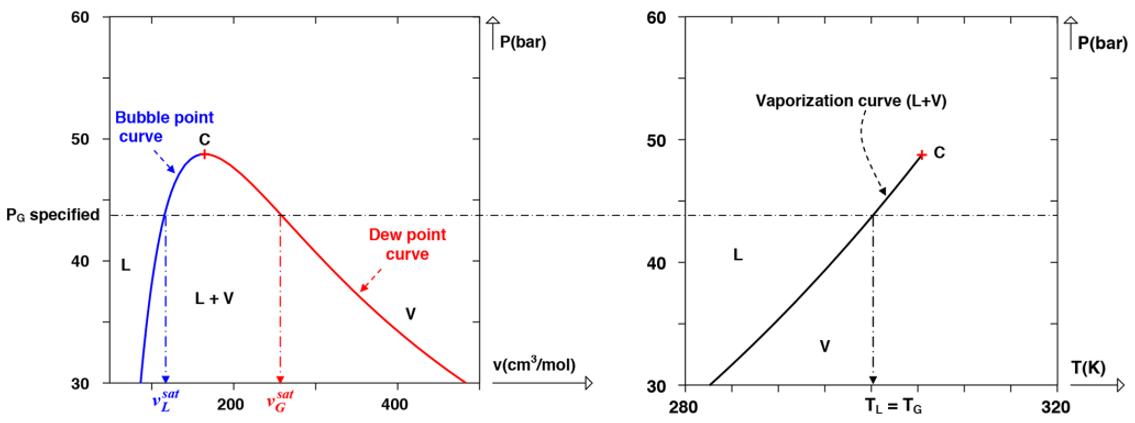
Let us now return to the example of a vapor–liquid pure substance for which we specified the pressure of the gas phase. We will illustrate on a graph the monovariant nature of this two-phase equilibrium. Figure 1.3 is a representation in the (P, ν) and (P, T) plane projections of the phase diagram of a given pure substance. The specification of the pressure PG of the gas phase in vapor–liquid equilibrium is shown by a horizontal dot-dash straight line.
Figure 1.3. Illustration of the Gibbs phase rule in the case of a pure substance in vapor–liquid equilibrium for which the pressure of the gas phase is specified. Left: phase diagram of a pure substance in the plane (P, v). Right: phase diagram in the plane (P, T). “L”: single-phase liquid domain, “V”: single-phase vapor domain, “L+V”: two-phase vapor–liquid domain; “C”: critical point
The () , Pv plane shows that by specifying GP , the following properties are then defined: (i) a unique molar volume for the liquid phase ( sat Lv ) defined by the intersection point of the bubble point curve (representing the vapor–liquid equilibrium pressure versus sat Lv ) and the horizontal straight line , PG P = (ii) a unique molar volume for the gas phase ( Gv ) found at the intersection of the dew point curve (representing the vapor–liquid equilibrium pressure versus sat Gv ) and the horizontal straight line PG P = The () , PT plane, on the other hand, shows that this specification induces also a unique vapor–liquid equilibrium temperature = LGTT (at the intersection of = PG P and the vaporization curve).
NOTE.– The temperature of a pure substance in vapor–liquid equilibrium is known as the boiling point temperature. When the pressure is specified, it is noted (). bp TP The normal boiling point temperature, denoted as , bpT ° is the boiling point temperature under normal pressure 1atm °= P , in other words 101,325 Pa.
Choice of the variable for correlations of phase-intensive properties for pure substances in vapor–liquid equilibrium: the previous paragraph insists on the need to set an intensive variable of a phase in order to characterize a vapor–liquid pure substance. In practice, often the temperature is chosen as the correlation variable. In doing so, the intensive properties of the phases are written: ()() = LG PTPT [pressures], (), sat G hT () sat L hT [molar enthalpies], (), sat L vT () sat G vT [molar volumes], ()() = satsat gLGTgT [molar Gibbs energies], etc.
NOTE.– The pressure of a pure substance in vapor–liquid equilibrium is known as the saturated vapor pressure. When the temperature is specified, it is written (). sat PT The molar volumes of the liquid and gas phases in vapor–liquid equilibrium are known as molar volumes of the saturated liquid and saturated gas phases, denoted respectively as () sat L vT and (). sat G vT
The definitions of the boiling point temperature (at a specified pressure) and of the saturated vapor pressure (at a specified pressure) are summarized in Figure 1.4.
Figure 1.4. Illustration of the definitions of the saturated vapor pressure and of the boiling point temperature in the pressure–temperature plane of a pure substance. VLE = vapor–liquid equilibrium, LSE = liquid–solid equilibrium, SVE = solid–vapor equilibrium
1.2.4.
Critical point of a pure substance
The critical point of a pure substance can be defined in three ways:
– in the (P, T) plane, it is the end point of the vaporization curve of a pure substance (see Figure 1.2);
– in the (P, ν) plane, this is the common maximum for the bubble point and dew point curves (see Figure 1.3);
– on the critical isotherm in the (P, ν) plane, it is a point of inflection with a horizontal tangent. This definition of the critical point is illustrated in the following section.
1.2.5.
Isotherms of a pure species in the fluid region
In the (P, ν) plane, an isotherm for a pure substance is a curve made up of all the (molar volume, pressure) couples associated with the same temperature.
Subcritical isotherms (subcritical means that the temperature is below the critical point temperature) are made up of three sections:
– a two-phase vapor–liquid domain: when the temperature is between the triple and critical temperatures, the pure substance has a unique vapor–liquid equilibrium pressure known as saturatedvaporpressure. In other words, at a fixed temperature, all the vapor–liquid states of a pure substance are isobaric; consequently, on an isothermal curve, a horizontal plateau (which shows states of the same pressure) characterizes the vapor–liquid equilibrium of the pure substance;
– a single-phase liquid domain: liquids under moderate pressure have the feature of being nearly incompressible (i.e. their molar volumes do not depend on pressure); as a result, the liquid single-phase domain of a subcritical isotherm can be roughly assimilated to a vertical straight line in the (P, ν) plane (liquid states are characterized by a same molar volume);
– a single-phase vapor domain: in the case of a pure substance under low pressure (typically 5bar < ), a gas phase can be assimilated to a perfect gas so that the pressure is given by the equation P = RT/ν. In the (P, ν) plane, the single-phase gas region of a subcritical isotherm can be assimilated to a branch of a hyperbolic curve.
By way of an illustration, two subcritical isotherms of ethane at T = 290 K and T = 300 K are represented in the (P, ν) plane in Figure 1.5 (left); on the right, we show the (P, T) plane for the pure substance in which the isotherms are vertical straight lines.
Figure 1.5. Representation of four isotherms (thin lines) of pure ethane in the (pressure, molar volume) plane (left) and (pressure, temperature) plane (right). C = critical point. The thick lines represent the intensive states of the phases in vapor–liquid equilibrium (bubble point curve, dew point curve, vaporization curve)
Bubble point curve = dew point curve (vaporization curve)
As the temperature is increased, the horizontal vapor–liquid equilibrium plateau in the () , Pv plane reduces: the molar volumes of the liquid and vapor phases in equilibrium move closer together (see Figure 1.5, left).
At the critical point C, these two phases have exactly the same molar volumes. In a more general way, at the critical point, the intensive properties of the liquid phase become identical to those in the gas phase. A critical isotherm is an isotherm drawn at the critical temperature of a pure substance (see the isotherm passing through C in Figure 1.5). On this curve (Figure 1.5, left), the vapor–liquid equilibrium plateau present at subcritical temperatures is reduced to a single point C. Geometrically, this induces the existence of an inflection point with a horizontal tangent on C. Mathematically, a critical point is characterized by the following two equations:
The quantity c v is called the criticalmolarvolumeofthepuresubstance.
Supercritical isotherms: since the critical point has been previously defined as the end point of the vaporization curve in the () , PT plane, it follows that at all temperatures higher than , c T the critical temperature, the pure substance remains single phase at all pressures; the isotherm in the () , Pv plane does not have a plateau associated with a change of state and looks approximately like a hyperbolic curve.
1.2.6. Property changes on vaporization
For all temperature ranging between the triple and critical temperatures, the molar property changes on vaporization are defined by: ()()() =− satsat vapGLXTxTxT Δ [1.9]
where sat Gx and sat L x denote the molar properties of the gas and liquid phases in vapor–liquid equilibrium respectively.
As an example, the molar volume of vaporization and the molar enthalpy of vaporization2 are defined by:
When the temperature becomes critical, the molar properties of the liquid and gas phases become identical; as a result, the properties of vaporization cancel each other out:
1.3. Correlations for the saturated vapor pressure of pure substances
1.3.1. Practical expressions for the saturated vapor pressure deduced from the Clapeyron equation
The Clapeyron equation is an exact relationship between the derivative of the saturated vapor pressure with respect to the temperature, on the one hand, and the enthalpy and volume of vaporization, on the other hand:
The temperature T is the absolute temperature (expressed in kelvin, for example). This equation can be used to deduce a mathematical expression for the () sat PT function. First, let us recall that the molar compressibility factor is defined as:
2 In practice, the molar adjective is often left out.
Consequently, the (molar) compressibility factor of vaporization is given by the expression:
The Clapeyron equation [1.12] can be rewritten using the quantity () vap ZT Δ :
Or equivalently:
This equation gives rise to a quantity B . Experimental measurements show that as a first approximation, B can be considered as constant. This statement is supported by Figure 1.6, which demonstrates the relative constancy of the B function with respect to the variations of the () vap HT Δ function.
Figure 1.6. Representation of the temperature variations of the adimensional functions of pure n-hexane ()/()vapc HTRT Δ , () vap ZT Δ and their ratio, denoted as /() c BRT
By integrating the relationship [1.16] with respect to the variable 1/ T and assuming a constant value of B , we obtain:
where A is a constant produced by the integration and () /K T is the absolute temperature expressed in kelvin (we point out that another unit of absolute temperature such as the Rankine scale would also have been suitable). Equation [1.17] is called the integratedformoftheClapeyron equation. This expression, involving two adjustable parameters (A and B) is indeed suitably adapted in practice to describe the saturated vapor pressures of pure substances over restricted temperature ranges. When this formula is applied to the entire domain ;,triplec TT
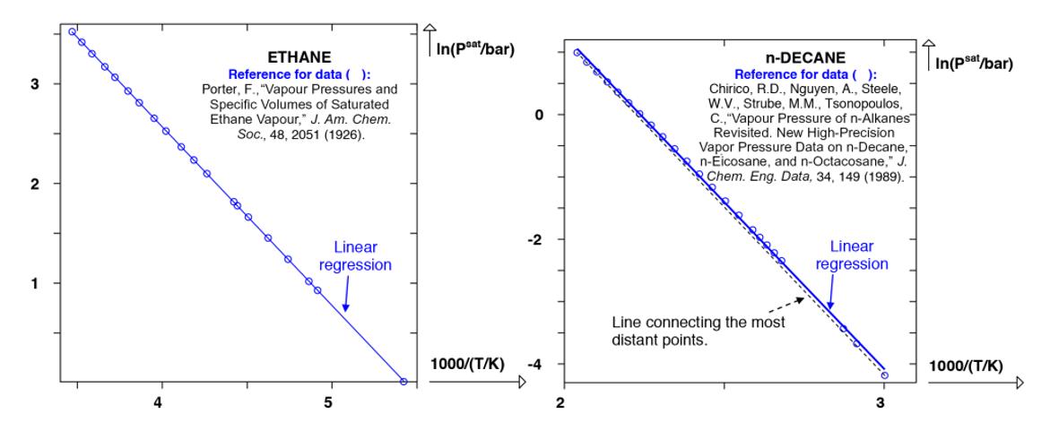
differences between the experimental and calculated points increase as the size of the molecule increases, as illustrated in Figure 1.7.
Figure 1.7. Representation of the natural logarithm of the saturated vapor pressure as a function of the inverse temperature in the case of ethane (left) and of n-decane (right). (O) experimental points; continuous lines: correlation
To determine the two parameters (A and B) of equation [1.17], it is sufficient to have two couples of points () 1/;ln. s TPat Free or commercial experimental databanks contain various types of data that allow determination of the two coefficients A and B . Some illustrations are given as follows:
– Let us suppose that we have the following data: (i) the normal boiling point temperature , bpT ° which is the boiling point temperature under a pressure of 1atm °= P , (ii) critical coordinates (),.cc TP If we assume that equation [1.17] is valid, the coefficients A and B are then the solutions to the system:
After resolution of the system [1.18], we obtain expressions for the coefficients A and B that can be inserted into equation [1.17]. When all calculations have been done, the following correlation is obtained:
– Let us now suppose that we dispose of the data: (i) () , cc TP and (ii) acentric factor .ω The definition of this property is provided below:
DEFINITION.– The acentric factor of a pure substance is defined by:
From the definition of the acentric factor, we deduce that the saturated vapor pressure of a pure substance at the temperature 0.7 c T is equal to ()
As previously seen, accepting the validity of equation [1.17] (rewritten by replacing natural logarithm by decimal logarithm), the coefficients A and B are then the solutions to the system:
After resolution of system [1.20], we obtain expressions for the coefficients A and B that, when reinserted into equation [1.17], lead to: