No part of this publication may be reproduced or transmitted in any form or by any means, electronic or mechanical, including photocopying, recording, or any information storage and retrieval system, without permission in writing from the publisher. Details on how to seek permission, further information about the Publisher’s permissions policies and our arrangements with organizations such as the Copyright Clearance Center and the Copyright Licensing Agency, can be found at our website: www.elsevier.com/permissions
This book and the individual contributions contained in it are protected under copyright by the Publisher (other than as may be noted herein).
Notices
Knowledge and best practice in this feld are constantly changing. As new research and experience broaden our understanding, changes in research methods, professional practices, or medical treatment may become necessary. Practitioners and researchers must always rely on their own experience and knowledge in evaluating and using any information, methods, compounds or experiments described herein. Because of rapid advances in the medical sciences, in particular, independent verifcation of diagnoses and drug dosages should be made. To the fullest extent of the law, no responsibility is assumed by Elsevier, authors, editors or contributors for any injury and/or damage to persons or property as a matter of products liability, negligence or otherwise, or from any use or operation of any methods, products, instructions, or ideas contained in the material herein.
Previous editions copyrighted 2015, 2002, 1995
Library of Congress Control Number: 2020941163
Content Strategist: Jennifer Catando
Senior Content Development Manager: Luke Held
Senior Content Development Specialist: Beth LoGiudice
Publishing Services Manager: Deepthi Unni
Project Manager: Janish Ashwin Paul
Design Direction: Patrick Ferguson
We dedicate this 4th edition to Dr. Thomas G. Nyland, an outstanding mentor and a founding father of veterinary ultrasound. We could not have done this without you.
J.S.M., C.R.B., and R.K.S.
EDITORS
John S. Mattoon, DVM, DACVR
Clinical Professor
Department of Veterinary Clinical Sciences College of Veterinary Medicine
Ultrasound-Guided Aspiration and Biopsy Procedures
Veterinary ultrasound has been evolving for nearly 40 years. Ultrasound has now become commonplace and an indispensable diagnostic tool for many in veterinary practice.
There have been phenomenal technical advances and the quality of current ultrasound equipment serves us at an indescribably high level compared with what we had when we frst began.
There is another frontier beyond high-quality equipment and its proper utilization, namely the integration of information gained from ultrasonography into the overall thought processes of clinicians in the diagnosis and management of patients. We believe this integration is the fnal piece to allow ultrasound to reach its fullest potential.
This 4th edition was written with the goal of moving us toward that potential. We have asked experts in internal medicine, oncology, emergency and critical care, surgery, ophthalmology, pathology, and cardiology to share their wisdom through these pages. We are delighted and inspired by the results. We hope you are as well.
As with all textbooks, the ultimate accountability for the content belongs to the editors and we accept responsibility for any and all errors that might appear in the text.
John S. Mattoon
Rance K. Sellon
Clifford R. Berry
First and foremost, we sincerely thank all of our contributors for this edition. You have provided invaluable insight and wisdom beyond our expectations. You have helped articulate how ultrasound can be effectively integrated into modern veterinary practice beyond technical utility.
Without contributors, colleagues, and friends from previous works, this 4th edition would never have been possible. Your contributions will never be forgotten and will always appreciated. It is hard to imagine it has been over 25 years since we started this journey and we cherish our time together along the way.
None of this is possible without the expertise, excellent guidance, and patience of the folks at Elsevier and partners. The helpfulness and understanding of Jennifer Catando, Luke Held, Beth LoGiudice, Erin Garner, Diane Chatman, Patrick Ferguson, Janish Paul, and
Santhoshkumar Govindaraju when times got tough cannot be underestimated or forgotten. Few people understand the effort it takes to produce a world-class publication. We sincerely thank you.
We are indebted as well to our families for their patience with us and support through the process of putting this textbook together. Finally, we are grateful to all of the mentors, teachers, colleagues, residents, and students that have taught each of us many of the things that are now a part of this textbook. We each stand on the shoulders of many giants of veterinary medicine.
Ultimately, it takes many people many hours to produce a textbook. We extend our heartfelt thanks to each and every one of you.
John S. Mattoon
Rance K. Sellon
Clifford R. Berry
1 Fundamentals of Diagnostic Ultrasound, 1
John S. Mattoon‚ Clifford R. Berry
2 Ultrasound-Guided Aspiration and Biopsy Procedures, 49
John S. Mattoon, Rachel Pollard, Tamara Wills, Clifford R. Berry
3 Point-of-Care Ultrasound, 76
Gregory R. Lisciandro
4 Abdominal Ultrasound Scanning Techniques, 105
John S. Mattoon‚ Clifford R. Berry
5 Eye, 138
Alison Clode‚ John S. Mattoon
6 Neck, 165
Dana A. Neelis‚ John S. Mattoon, Rance K. Sellon
7 Thorax, 199
Dana A. Neelis‚ John S. Mattoon, Megan Grobman
8 Echocardiography, 230
John D. Bonagura, Virginia Luis Fuentes
9 Liver, 355
Martha Moon Larson, John S. Mattoon, Yuri Lawrence, Rance K. Sellon
10 Spleen, 422
John S. Mattoon‚ Megan Duffy
11 Pancreas, 461
John S. Mattoon‚ Jennifer E. Slovak, Rance K. Sellon
12 Gastrointestinal Tract, 491
Dana A. Neelis‚ John S. Mattoon‚ Jennifer E. Slovak, Rance K. Sellon
13 Peritoneal Fluid, Lymph Nodes, Masses, Peritoneal Cavity, and Great Vessel Thrombosis, 526
William R. Widmer‚ John S. Mattoon, Rance K. Sellon
14 Musculoskeletal System, 544
Ashley Hanna‚ Tina Owen, John S. Mattoon
15 Adrenal Glands, 566
Dana A. Neelis, John S. Mattoon, Rance K. Sellon
16 Urinary Tract, 583
William R. Widmer, John S. Mattoon, Shelly L. Vaden
17 Prostate and Testes, 635
John S. Mattoon, Autumn Davidson
18 Ovaries and Uterus, 665
John S. Mattoon, Autumn Davidson, Rance K. Sellon
Index, 689
INSTRUCTIONAL “HOW-TO” VIDEOS
How to perform an abdominal ultrasound
How to perform a cardiac ultrasound
ABDOMINAL ULTRASOUND SCANNING TECHNIQUES
Sagittal ultrasound scans of the liver in two normal dogs
Dorsal to transverse scans of the mid-liver in two normal dogs
Dorsal to transverse scans of the right and left portions of the liver in a normal dog
Ultrasound evaluation of the canine spleen
Ultrasound evaluation of the stomach
Ultrasound evaluation of the pancreas
Ultrasound evaluation of the kidneys
Ultrasound evaluation of the adrenal glands
Ultrasound evaluation of the urinary bladder
Prostate gland in a young intact beagle dog
Ovaries and uterus in a young beagle dog
ULTRASOUNDS OF THE EYE
Power Doppler examination of persistent hyaloid artery
Retrobulbar grass awn (foxtail) cellulitis
ULTRASOUNDS OF THE NECK
Thyroid carcinoma
Calcifed thyroid carcinoma
Esophageal abscess
ULTRASOUNDS OF THE THORAX
Normal gliding lung
Pneumonia
ULTRASOUNDS OF THE HEART
Right parasternal long-axis imaging
Right parasternal short-axis imaging
Imaging of the pulmonary artery
Left apical images
Images of the right heart
Subcostal image of the heart
M-mode examination
Saline contrast echocardiography
Transesophageal echocardiography (TEE)
3D imaging
Normal Doppler imaging of blood fow
Myocardial Doppler and deformation imaging
Tissue Doppler imaging
Spectral Doppler echocardiography
Color Doppler fow Shunts
Valvular stenosis
Valvular regurgitation
VIDEO CONTENTS
2D and M-mode examples of cardiomegaly
Enlargement of the great vessels
Methods for estimating left ventricular ejection fraction
Mitral regurgitation
Complementary image planes
Effects of control settings on color images
Mitral valve malformations
Myxomatous valvular disease in dogs
Infective endocarditis
Left atrial tears
Ventricular systolic function
Tricuspid valve disease
Aortic regurgitation
Cor triatriatum dexter
Aortic stenosis
Pulmonary stenosis
Double-chambered right ventricle
Pulmonary hypertension
Cardiomyopathy
Hypertrophic
Restrictive
Dilated
Preclinical dilated
Right ventricular
Pericardial diseases and cardiac-related tumors
Atrial septal defects
Ventricular septal defects
Patent ductus arteriosus
ULTRASOUNDS OF THE LIVER
Normal dog liver
Biliary sludge and cholecystitis
Common bile duct obstruction
Right divisional portosystemic shunt
Portal vein thrombus
ULTRASOUNDS OF THE SPLEEN
Splenic hyperplasia
Hyperechoic splenic lipomas
Diabetes and pituitary-dependent hyperadrenocorticism
ULTRASOUNDS OF THE PANCREAS
Acute pancreatitis
Acute pancreatitis and peritonitis
Enlarged and misshapen left lobe of the pancreas
Pancreatic abscess and peritonitis
Neuroendocrine tumor (insulinoma)
ULTRASOUNDS OF THE GASTROINTESTINAL TRACT
Pylorus to duodenum
Fine-needle aspiration of the stomach wall
Gastric leiomyosarcoma in a dog
Gastric lymphoma in a dog
Small intestinal dilation secondary to linear foreign body obstruction in a cat
Intussusception
Adenocarcinoma of the small intestine in a dog
Adenocarcinoma of the small intestine with metastasis to mesentery
Leiomyoma of the small intestine
ULTRASOUNDS OF THE PERITONEAL CAVITY
Aortic thrombus
Caudal vena cava thrombus
ULTRASOUNDS OF THE ADRENAL GLANDS
Left adrenal glands
Right adrenal glands
Large left adrenal mass in a geriatric dog
Right adrenal gland tumor with development of large caudal vena cava thrombus
ULTRASOUNDS OF THE URINARY TRACT
Normal kidney blood fow
Kidney masses in a dog
Kidney masses in a cat
Hydronephrosis
Ureters with ureteral calculus
Renal vein
Ureteral jet
Hydronephrosis, hydroureter, and ureterocele
Urinary bladder mass
Masses in urinary bladder and kidney, hydronephrosis, and renal cyst
Thickening and heterogeneity of the apical bladder wall
ULTRASOUNDS OF THE PROSTATE AND TESTES
Bacterial prostatitis with perineal swelling
Bacterial prostatitis with mineralization
Prostatic carcinoma with ureteral obstruction
Paraprostatic cyst and benign prostatic hyperplasia with a perineal hernia
ULTRASOUNDS OF THE OVARIES AND UTERUS
Ovary and uterine horn (transverse)
Ovary and fetus
Ovarian follicle
Ovary and uterine horn (sagittal)
Cystic endometrial hyperplasia (CEH)-mucometra
Pregnancy after cystic endometrial hyperplasia (CEH)-mucometra
Uterine stump hematoma
Fundamentals of Diagnostic Ultrasound
John S. Mattoon‚ Clifford R. Berry
Diagnostic ultrasound uses high-frequency sound waves that are pulsed into the body, and the returning echoes are then analyzed by computer to yield high-resolution cross-sectional images of organs, tissues, and blood fow. The displayed information is a result of ultrasound interaction with tissues, which is based on the tissue’s acoustic impedance, and does not necessarily represent specifc microscopic or macroscopic anatomy. Indeed, organs may appear perfectly normal on an ultrasound image in the presence of dysfunction or failure. Conversely, organs may appear abnormal on the ultrasound examination but be functioning properly. This basic tenet must be understood and respected for diagnostic ultrasound to be used properly.
High-quality ultrasound studies require a frm understanding of the important physical principles of diagnostic ultrasound. In this introductory chapter, we strive to present the necessary fundamental physical principles of ultrasound without excessive detail. In-depth sources on the subject are recommended to interested readers.1-5 These textbooks uniformly stress that image quality depends on knowledge of the interaction of sound with tissue and the skillful use of the scanner’s controls. Ultrasound examinations are highly interactive; a great deal of fexibility is often required for good images to be obtained. Accurate interpretation depends directly on the differentiation of normal and abnormal anatomy. Unlike with other imaging modalities, interpretation is best made at the time of the study. It is very diffcult to render a meaningful interpretation from another sonographer’s static images or video clips.
BASIC ACOUSTIC PRINCIPLES
Wavelength and Frequency
Sound results from mechanical energy propagating through matter as a pressure wave, producing alternating compression and rarefaction bands of molecules within the conducting medium (Fig 1 1). The distance between each band of compression or rarefaction is the sound’s wavelength (l), the distance traveled during one cycle. Frequency is the number of times a wavelength is repeated (cycles) per second and is expressed in hertz (Hz). One cycle per second is 1 Hz; 1000 and 1 million cycles per second are 1 kilohertz (kHz) and 1 megahertz (MHz), respectively. The range of human hearing is approximately 20 to 20,000 Hz. Diagnostic ultrasound is characterized by sound waves with a frequency up to 1000 times higher than this range. Sound frequencies in the range of 2 to 15 MHz and higher are commonly used in diagnostic ultrasound examinations. Even higher frequencies (20 to 100 MHz) are used in special ocular, dermatologic, and microimaging applications.
Frequencies in the millions of cycles per second have short wavelengths (submillimeter) that are essential for high-resolution imaging.
The shorter the wavelength (or higher the frequency), the better the resolution. Frequency and wavelength are inversely related if the sound velocity within the medium remains constant. Because sound velocity is independent of frequency and nearly constant (1540 m/sec) in the body’s soft tissues1,5 ( Table 1.1), selecting a higher frequency transducer will result in decreased wavelength of the emitted sound, providing better axial resolution (see Fig. 1.1, A, and Fig. 1.2). The relationship between velocity, frequency, and wavelength can be summarized in the following equation:
Velocity frequency wav (m/sec) (cycles/sec) eelengthm/cycle()
The wavelengths for commonly used ultrasound frequencies can be determined by rearranging this equation ( Table 1 2).
Propagation of Sound
Diagnostic ultrasound uses a “pulse echo” principle in which short pulses of sound are transmitted into the body (see Fig. 1.1, C). Propagation of sound occurs in longitudinal pressure waves along the direction of particle movement as shown in Fig. 1.1. The speed of sound (propagation velocity) is affected by the physical properties of tissue, primarily the tissue’s resistance to compression, which depends on tissue density and elasticity (stiffness). Propagation velocity is increased in stiff tissues and decreased in tissues of high density. Fortunately, the propagation velocities in the soft tissues of the body are very similar, and it is therefore assumed that the average velocity of diagnostic ultrasound is 1540 m/sec.
The ultrasound transducer both sends pulses into the tissue (1% of the time) and receives the returning echoes (99% of the time). The assumption of a constant propagation velocity (1540 m/sec) is fundamental to how the ultrasound machine calculates the distance (or depth) of a refecting surface. Suppose it takes 0.126 msec from the time of pulse until the return of the echo. The depth of the refective surface would be calculated as follows:
This value must be divided by 2 to account for the round trip to and from the refector, so the depth of the refective surface equals 9.70 cm.
It should be intuitive then that if the sound travels through fatty tissue at 1450 m/sec, the refector depth will be erroneously calculated as greater (or deeper) than it actually is. This is termed the speed propagation error and is discussed and illustrated further in later sections that focus on artifacts.
Fig. 1.1 Ultrasound waves and echoes. A, Ultrasound emitted from the transducer is produced in longitudinal waves consisting of areas of compression (C) and rarefaction (R) B, The wavelength, depicted overlying the longitudinal wave, is the distance traveled during one cycle. Frequency is the number of times a wave is repeated (cycles) per second. The wavelength decreases as frequency increases. Switching from a lower frequency to a higher frequency transducer (e.g., from 3.0 to 7.5 MHz) shortens the wavelength and provides better resolution. C, In pulsed ultrasound systems, sound is emitted in pulses of two or three wavelengths rather than continuously as seen in A and B. A portion of the sound is refected, whereas the remainder is transmitted as it passes through interfaces in tissues.
TABLE 1.1 Velocity of Sound in Body Tissues
Data from Curry TS III, Dowdey JE, Murry RC Jr. Christensen’s Physics of Diagnostic Radiology. 4th ed. Philadelphia: Lea & Febiger; 1990.
*Assumes 3 wavelengths/pulse
Fig. 1.2 Axial resolution. Higher frequency transducers produce shorter pulses than lower frequency transducers because the wavelength of the emitted sound is shorter. Pulse length actually determines axial resolution and is directly dependent on the wavelength from the primary ultrasound beam. In this example, the near and far walls of a cyst can be resolved if the echoes returning to the transducer from each wall remain distinct. The echo from the near wall must clear the wall before the echo from the far wall returns to merge with it. The ability to resolve the cyst is dependent on the pulse length and distance between walls. Axial resolution cannot be better than half the pulse length. In this example, a 0.5-mm cyst could theoretically be resolved with a 7.5-MHz but not a 3.0-MHz transducer because of the superior axial resolution of the higher frequency.
TABLE 1.2 Commonly Used Ultrasound Frequencies*
*Assume velocity 5 1.54 mm/µsec (1540 m/sec).
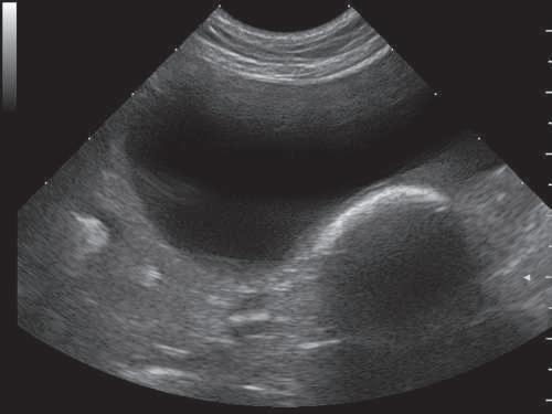
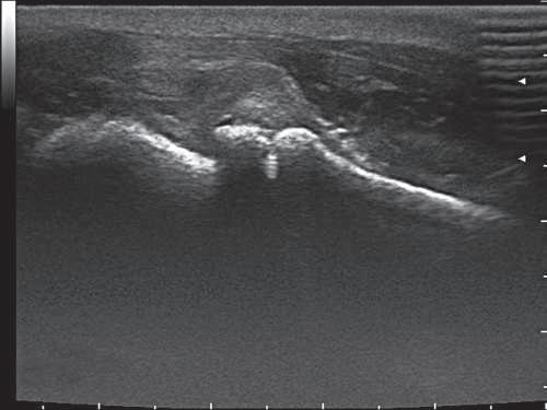
Fig. 1.3 Strong refectors of ultrasound. A, Gas and faecal material within the descending colon (arrow) creates a very echogenic, curved interface deep to the anechoic urinary bladder. Secondary lobe artifacts are present, creating false echoes within the normally anechoic urine. Acoustic shadowing is present deep to the colon. It is not as complete (clean) a shadow as that created by mineral. B, The body surface of the proximal humerus, supraglenoid tubercle (SGT), and scapula are highly refective, creating a vividly hyperechoic outline of the left shoulder of this puppy with septic arthritis. There is a reverberation artifact in the upper right corner of the image created by poor transducer-skin contact (arrowheads). Acoustic shadowing is present deep to the bone surfaces.
Further, when the ultrasound beam encounters gas (331 m/sec) or bone (4080 m/sec), marked velocity differences in these media result in high refection and improper echo interpretation with characteristic reverberation and shadowing artifacts (see later sections on artifacts) (Fig 1 3). This strong refection is a result of a combination of an abrupt change in sound velocity and the physical density of the media (defned as the acoustic impedance) at a soft tissue–bone or soft tissue–air interface. Acoustic impedance is discussed later in this chapter.
The depth to which sound penetrates into soft tissues is directly related (but inversely proportional) to the frequency employed. Higher frequency sound waves are attenuated more than lower frequency waves, so attempts to improve resolution by increasing frequency result in decreased penetration. By recognizing this important inverse relationship, the ultrasonographer selects the highest frequency transducer that will penetrate to the desired depth. Standard microconvex curved-array transducers imaging between 8 and 11 MHz should be expected to penetrate suffciently for high-quality images to a depth of 8 to 10 cm.
Refection and Acoustic Impedance
The echoes refected from soft tissue interfaces toward the transducer form the basis of the ultrasound image. Interfaces that are large relative to beam size are known as specular refectors. Interfaces that are not at a 90-degree angle to the ultrasound beam refect sound away from the transducer and do not contribute to image formation. Therefore scanning from different angles may improve image quality as different interfaces become perpendicular to the beam. An example illustrating the importance of a 90-degree incidence angle is shown in Fig 1 4
The velocity of sound within each tissue and the tissue’s physical density determine the percentage of the beam refected or transmitted as it passes from one tissue boundary to another or to different boundaries within a given tissue. The product of the tissue’s physical density and the sound velocity within the tissue is known as the tissue’s acoustic impedance, which refers to the refection or transmission characteristics of a tissue. For simplifcation, the physical density differences between tissues can be used to estimate acoustic impedance in soft
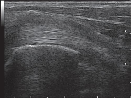
Fig. 1.4 Importance of angle of incidence of the ultrasound beam. Multiple, parallel, echogenic fbers of the biceps tendon are well visualized across the center of the image because the ultrasound beam is perpendicular (90 degrees) to them. As the tendon bends away to the right and left, the echogenicity of the tendon is lost (arrowheads). The ultrasound beam is now off-incidence (no longer perpendicular) to the tendon, refracted away. This artifact could be mistaken for tendon pathology.
tissue because sound velocity is assumed to be nearly constant. Acoustic impedance can be defned by the following equation:
It is the difference in acoustic impedance between the tissues that accounts for the refectivity of a given tissue. The amplitude of the returning echo is proportional to the difference in acoustic impedance between two tissues as the sound beam passes through their interface. There are only small differences in acoustic impedance among the body’s soft tissues ( Table 1 3).6 This is ideal for imaging purposes because only a small percentage of the sound beam is refected at such
LF BICEPS SAG
TABLE 1.3 Acoustic Impendence
of organs, scattering occurs. This is also termed diffuse refection or nonspecular refection and is independent of beam angle. Acoustic impedance mismatches are small compared with those of specular refectors, and the returned weak echoes can be imaged only because they are abundant and tend to reinforce one another, producing ultrasound speckle. These echoes contribute to the parenchymal echotexture seen in abdominal organs but may not represent actual anatomy, gross or microscopic. This type of scattering increases with higher frequency transducers so that echotexture, and thereby detail, is appreciably enhanced.
Refraction
Data from Curry TS III, Dowdey JE, Murry RC Jr. Christensen’s Physics of Diagnostic Radiology. 4th ed. Philadelphia: Lea & Febiger; 1990. *Acoustic impedance (Z) 5 3106 kg/m2-sec.
TABLE 1.4 Sound Refection at Various Interfaces
Data from Hagen-Ansert SL. Textbook of Diagnostic Ultrasonography. 3rd ed. St Louis: Mosby; 1989.
interfaces, whereas the majority is transmitted and available for imaging deeper structures.
Bone and gas have high and low acoustic impedances, respectively. Air is less dense and more compressible than soft tissue and transmits sound at a lower velocity. Bone is more dense and less compressible than soft tissue and transmits sound at a higher velocity. This means that when the ultrasound wave encounters a soft tissue–bone or soft tissue–gas interface, nearly all of the ultrasound waves are refected and little is available for imaging deeper structures ( Table 1 4; see Fig. 1.3). This effect represents a high acoustic impedance mismatch. Distal acoustic shadowing is produced deep to the bone or gas because little sound penetrates. Increasing output intensity, decreasing frequency, or increasing gain will not improve penetration but merely increase artifacts, such as reverberation echoes (as seen with a soft tissue–gas interface). The sonographer must fnd an “acoustic window” that avoids bone and gas when imaging the abdomen. For the same reason, an acoustic coupling gel is used between the transducer and skin for all ultrasound examinations to eliminate interposed air.
Scattering and Speckle
Most echoes displayed on the ultrasound image do not arise from large specular refectors, such as the surface of organs, but from within the organs. When the ultrasound beam encounters small uneven interfaces less than the incident wavelength (submillimeter) in the parenchyma
The velocity change occurring as a sound wave passes from one medium to another causes the ultrasound beam to bend if the interface between the media is struck at an oblique angle. This can produce an artifact of improper location for an imaged structure. Altering the ultrasound beam’s direction in the tissues is called refraction. Refraction, along with refection, also contributes to a thin, echo-poor area that is lateral and distal to curved structures, such as the gallbladder, edge of the urinary bladder or kidneys, or a cyst (Fig. 1.5). This artifact is termed an edge shadow.
Attenuation
The ultrasound beam is transmitted into the body as acoustic energy, quantifed as acoustic power (P) expressed in watts (W) or milliwatts (mW) per unit time, or intensity (I), which accounts for the crosssectional area of the ultrasound beam (I 5 W/cm2). Attenuation is the collective term that describes the loss of acoustic energy as sound passes through tissues. Echoes refected back toward the transducer are also attenuated in an identical manner. Sound attenuation (physical ultrasound wave loss) is generally measured in decibels (dB) rather than intensity or power.
Factors that contribute to attenuation are absorption (heat loss), refection, and scattering of the sound beam. Absorption refers to conversion of a sound pulse’s acoustic (mechanical) energy to heat. This is primarily a result of frictional forces as the molecules of the transmitting medium move back and forth longitudinally in response to the passage of a sound wave. Heat production within tissues is important
Fig. 1.5 Refraction of ultrasound. Refraction of the ultrasound beam produces a shadow distal to curved structures. The structure must propagate sound at a velocity different from that of the surrounding medium. This phenomenon is often referred to as critical-angle shadowing or edge shadowing. Outward refraction of the beam is seen when the sound velocity is higher in the structure than in the surrounding medium. This occurs when sound passes from retroperitoneal fat through the curved surface of the kidney. In the case of a liver or kidney cyst, sound refraction is inward (focused) because velocity within the cyst is lower than in liver or kidney tissue. Distal enhancement (E) is also seen deep to cysts because of a decreased attenuation within the cyst compared with surrounding tissue.
when the biological effects and safety of the ultrasound are considered. Nevertheless, in the diagnostic imaging range, heating is negligible because the acoustic power is restricted on each imaging machine (see the later section about the pulser).
Of great importance is that the amount of attenuation is directly proportional to the frequency of the ultrasound beam; higher frequencies are attenuated much more than lower frequencies in a given medium. This means that any attempt to improve resolution by increasing the frequency invariably decreases penetration. The attenuation is substantial and is equal to approximately 0.5 dB/cm/MHz in soft tissues over the round-trip distance. This is an essential concept because it dictates transducer selection, overall and depth (or time) dependent gain settings, and system power.
Dark areas (shadowing) are noted distal to highly attenuating structures (mineral, air), whereas lighter areas (acoustic enhancement) are seen distal to tissues with low sound attenuation (fuid). Some disease processes, such as severe hepatic lipidosis in cats, diffuse vacuolar hepatopathy in dogs, and fat-induced steatitis in dogs or cats with severe pancreatitis, cause abnormal attenuation of ultrasound beams in soft tissues.
INSTRUMENTATION
All diagnostic ultrasound machines, regardless of cost or features, consist of several basic components. A pulser energizes piezoelectric crystals within the transducer, emitting pulses of ultrasound into the body. Returning echoes are received by the same piezoelectric crystals arranged along the transducer surface and are converted to a digital signal to form the image that is viewed on a monitor.
Pulser
Ultrasound imaging is based on the pulse-echo principle. This means that sound is produced by the transducer in pulses rather than continuously (see Figs. 1.1 and 1.2). The pulser (or transmitter) applies precisely timed high-voltage pulses to the piezoelectric crystals within the transducer, which then emits short bursts of ultrasound into the body. The image is formed from the echoes returning to the transducer from the tissues after each pulse. Therefore adequate time must be allowed for all echoes to return before the transducer is pulsed again. Typically, sound is transmitted less than 1% of the time; the transducer is waiting for all echoes to return more than 99% of the time. When the crystal is pulsed, approximately two or three wavelengths are emitted in each pulse before a backing block in the transducer dampens the vibration. Thus the spatial pulse length is commonly two or three wavelengths. A higher frequency transducer emits shorter wavelengths, and therefore correspondingly shorter pulses, than a lower frequency transducer (see Figs. 1.1 and 1.2). It is the pulse length, which is in turn dependent on the transducer frequency, that determines the ability to separate points along the axis of the sound beam, termed axial resolution. The pulse length is commonly 0.1 to 1.0 mm. Axial resolution cannot be better than half the pulse length because of the overlap of returning echoes refected off closely spaced interfaces.1
There are two points of clinical importance with regard to the pulser. One is that the ultrasonographer can adjust the voltage applied to the transducer by using the power control. The power control is a volume control that adjusts the acoustic energy (or loudness, in decibels) that is transmitted into the body. The louder the pulses going into the body, the louder the returning echoes, which in turn creates an overall brighter image. The power control is the only operator adjustment that affects sound transmitted into the body. All other controls affect the returning echoes at the level of the receiver. Although it would be useful to have unlimited acoustic energy so that image
brightness would never be an issue, the U.S. Food and Drug Administration (FDA) regulates the maximum output of ultrasound scanners for patient safety. The permissible acoustic energy in part depends on the type of examination selected. For example, settings used with pediatric subjects have a lower maximum output than those used with adults.
The other important point is that the rate of the pulses can also be controlled; this is termed pulse repetition frequency (PRF). It is fundamentally important that the time between ultrasound pulses be long enough to allow returning echoes to reach the transducer before the next pulse of sound is emitted. If a pulse of transmitted sound occurs too soon, overlap with the returning echoes creates erroneous data. This requirement is particularly signifcant when using Doppler ultrasound, which is explained later in the chapter. For reference, PRFs of less than 1 to 10 kHz or higher are necessary in diagnostic ultrasound, meaning that a diagnostic pulse is created every .001 to .0001 seconds.
Transducer
The transducer (commonly referred to as a scan head or probe) plays the dual role of transmitter and receiver of ultrasound through use of piezoelectric crystals. As noted, piezoelectric crystals vibrate and emit sound when voltage is applied to them by the pulser. The range of frequencies emitted by a particular transducer depends on the characteristics and thickness of the crystals contained within the scan head.
Modern transducers are capable of multifrequency operation, termed broad bandwidth. A range of frequencies are produced, composed of a preferential (central) frequency in addition to higher and lower frequencies. Advances in transducer technology allow simultaneous imaging of the near and far felds with sound waves of different frequencies. This allows the maximal resolution possible for a given depth without having to switch transducers. The use of broad bandwidth technology has several advantages. From a practical standpoint, the transducer may be operated at higher or lower frequencies for increased resolution or increased penetration for deeper structures, respectively (Fig. 1.6). It has also allowed manufacturers to achieve better image resolution by capturing the spectrum of frequencies produced by insonated tissues. Speckle artifact can be reduced by frequency compounding, a technique that adds together speckle patterns generated at different frequencies, resulting in an increase in image contrast.
Receiver
When the piezoelectric crystals within the transducer encounter acoustic pressure waves from returning echoes, small voltages are produced. These electrical signals are processed by the ultrasound computer (the receiver), ultimately creating a diagnostic image. Manipulating these weak electrical signals by selecting various scanner controls (processing parameters) to create the best possible image is largely operator dependent and constitutes the “art” of diagnostic ultrasound.
Scanner Controls
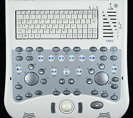
Scanner controls permit the operator to maximize image quality; less than ideal or improper settings degrade the image. Importantly, adjustments may directly affect image interpretation. Organs can be made hyperechoic or hypoechoic, or their parenchymal texture may be displayed as course or fne, depending on the selection and adjustment of the many operator controls. Controls are given a variety of names, depending on the manufacturer (Fig. 1.7), but their functions are similar despite the inconsistency in names. Understanding and learning to effectively operate ultrasound equipment is one defning difference between experienced and inexperienced sonographers.
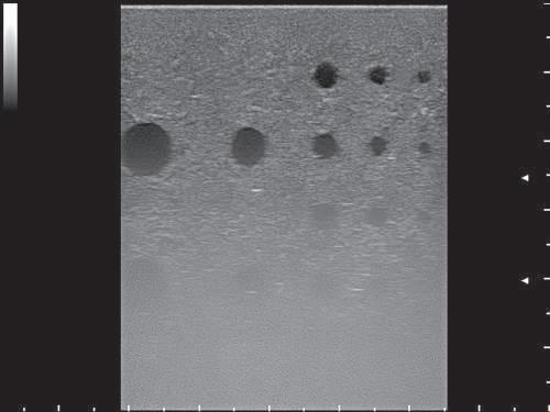
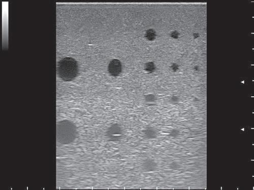
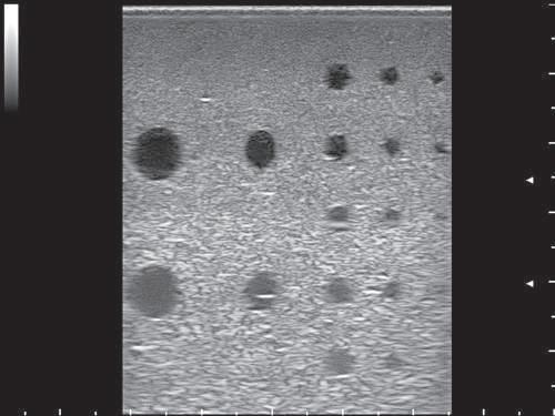
Fig. 1.6 Broadband transducer frequency effect on image quality and depth penetration. A linear-array broadband (4 to 13 MHz) transducer was used to make these images of an ultrasound phantom. The only parameter difference between images is the portion of the frequency range selected (high, mid, and low). Two focal points are present, at depths of 2.5 and 4 cm. Overall depth of the displayed image is 5.9 cm. A, Operating at 13 MHz, there is good visualization of the frst two rows of cysts in the near feld, at depths of 1 and 2 cm. Poor depth penetration of the high frequency 13 MHz selection does not allow adequate ultrasound beam penetration for visualization of the deeper rows of cysts, located at 3, 4, and 5 cm. B, Operating at midband of the frequency spectrum there is better penetration of the ultrasound beam to 5 cm, allowing recognition of the deeper cysts. Note how the deeper tissue has become brighter. C, At the lower frequency range (4 MHz), the cysts at 4 and 5 cm are more clearly seen and the overall image is brighter.
There is only one control to alter the intensity of sound output from the transducer (the power control); all other controls are used to adjust amplifcation of the returning echoes. Gain and time-gain compensation (TGC) controls are the most important operator controls, and these must be mastered to yield the best possible image. Additionally, they must be adjusted throughout an examination to account for differences in the depth of a particular structure in the patient and the area examined (e.g., liver versus urinary bladder). There are a plethora of additional controls used to optimize the image. These include dynamic range, gray-scale display maps, edge flters, persistence, and scan line density. Fig. 1.8 illustrates many of the controls as indicated on the image display screen.
Ultrasonography is based on the pulse-echo principle, as discussed previously. A pulse of sound is emitted from the transducer after a special piezoelectric crystal contained within the scan head is vibrated and quickly dampened. The PRF is the number of pulses occurring in 1 second, typically in the thousands of cycles per second. The
frequency of sound emitted depends on a crystal’s inherent characteristics. The crystal’s vibrations are immediately dampened by a backing block so that only a short pulse length of two or three wavelengths is emitted. The crystal then remains quiet as it waits for returning echoes refected from tissues within the body. These echoes vibrate the crystal again, producing small voltage signals that are amplifed to form the fnal image.
A timer is activated at the moment the crystal is pulsed so that the time of each echo’s return can be determined separately and placed at the appropriate location on the video monitor. The elapsed time represents the distance (depth) from the transducer where a particular echo originated. An average speed of sound within soft tissues (approximately 1540 m/sec) is assumed by all ultrasound equipment. The elapsed round-trip time must be halved and multiplied by 1540 m/sec to determine the actual distance of the refecting interface from the transducer (Fig. 1.9). Therefore echoes arising from the deepest tissues return to the transducer later than those from superfcial
Fig. 1.7 Ultrasound operator controls. The sonographer must become familiar with the controls so that image optimization becomes routine. The controls are labeled with text or icons for easy identifcation of function. An alphanumeric keyboard is seen in the top of the image. To the right are the time-gain compensation (TGC) controls. The large wheel on the right is the gain control for brightness (B-) and motion (M)-mode, and the power toggle is seen at upper right. Doppler controls are centered around the gain wheel on the left and the lower row of blue toggle switches. Familiarity with personal computers should allow most operators to become comfortable with the controls in a relatively short time despite the rather ominous array of knobs and switches.
(MyLab 30, Biosound Esaote, Indianapolis, IN)
structures. A dot representing each returning echo is placed on the video monitor at the appropriate depth according to the time it took for the echo to go out into the tissue and return. Ultrasound instruments are calibrated to interpret and display the depth in centimeters (rather than time of return) automatically. A gray-scale value is also assigned to each pixel of the image corresponding to the amplitude or strength and number of the returning echoes. The current convention is to display low-intensity echoes as nearly black, medium-intensity echoes as various shades of gray, and high-intensity echoes as white (white-on-black display).
The human eye can distinguish only about 10 to 12 shades of gray on a video monitor. Most ultrasound systems are designed to acquire a wider range of levels (128 to 512 levels or more) and ft them into the dynamic range of the monitor by using special compression, expansion, or mapping schemes. Images can be postprocessed so that shades of gray can be assigned in various ways from the acquired signals. When gray levels are assigned, priority can be given to weaker signals so that subtle changes in parenchymal refection amplitude are represented by separate shades of gray. Conversely, strong signals can be assigned more gray values when weaker echoes are unimportant. The resultant change in image contrast theoretically displays only the most clinically relevant information. Operator-selectable postprocessing curves using linear or logarithmic functions are preinstalled on many machines. In some cases, the curves can be customized by the sonographer. The curve and contrast setting that best suits the application and the ultrasonographer can then be saved as a preset so that repeated manipulations are not necessary for each study.
The ultrasound beam and the returning echoes are attenuated as they pass through tissues. The farther away a refecting interface is from the transducer, the weaker the returning echo will be. The ultrasound scanner’s controls are designed to either increase the intensity
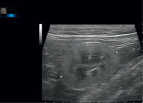
Fig. 1.8 Screen information: deciphering displayed ultrasound parameters. An explanation of the letters and numbers depicted on the ultrasound image is offered here to help demystify the plethora of postprocessing controls available. Adjustment allows the image to be fnetuned. Each manufacturer has its own nomenclature and method of information display, but there is commonality in function. In this sagittal image of the left kidney (LK) the transducer indicator is directed cranially; thus the cranial pole of the left kidney is to the left and caudal to the right. All manufacturers have some form of transducer mark that corresponds to a symbol on the edge of the image, usually the company icon. A wide-band high-frequency (4 to 13 MHz) linear-array transducer has been used for these images (designated LA523). The transducer is being operated the higher end of its frequency range, indicated by the small bar graph position (toward 13) in the far upper left icon, and the B RES-L denotation (B-mode, RES 5 resolution, L 5 lower part of the highest frequency range) within the upper left header. Just below this is the total depth of feld, D 44 mm. Two focal points have been used (small white arrowheads along the right margin) to maximize resolution at the depth of the kidney. The small tick marks along the right y-axis and the x-axis represent 5 mm increments; the larger tick marks indicate 1 cm. PRC 16/1/2: This denotes three different image processing programs and the corresponding machine settings. P 5 dynamic range, 16. Dynamic range is the difference in loudness between the weakest returning echoes and the strongest. (A higher dynamic range yields more shades of gray, whereas a lower dynamic range yields a more black and white image (higher contrast). Abdominal imaging uses a wider dynamic range, whereas in cardiology a narrower range is used to maximize contrast. Tendon and ligament examinations are often optimized in between. On this machine, dynamic range is indicated in numerals.) On others, the value is given in decibels (dB). A wide dynamic range could be 90 dB and a narrow range could be 50 dB. R 5 enhancement, 1. Enhancement is a setting to increase or decrease edge defnition. C 5 line density, 2. Line density is the number of ultrasound scan lines shown. Increasing the line density increases detail; decreasing line density results in a faster frame rate at the expense of image detail. PST 0: Indicates the gray-scale map selected. G —: Indicates the gain setting, not displayed on a captured image. XV 2: Denotes “X View,” a proprietary imageviewing program. PRS 5: Persistence level. Persistence is how long each successive frame is overlapped with the next image frame. A long persistence yields a very smooth image, and excessive persistence results in a blurred image. C 2: Denotes dynamic contrast. D1 3.45 cm: The measurement of the left kidney (LK) length, between the electronic cursors. (MyLab 30, Biosound Esaote, Indianapolis, IN)
of sound transmitted into tissues (power control) or electronically amplify returning echoes to compensate for this attenuation. These are the depth-gain and time-gain compensation (DGC or TGC, respectively) controls. In most cases, the TGC controls are also used to suppress strong echoes returning from superfcial structures in the near
Interface distance == 50 mm V RT 2
V = 1540 m/sec = 1.54 mm/ sec
(Average speed of sound in soft tissue)
RT = 65 sec
Fig. 1.9 Distance determination by round-trip time. The ultrasound scanner determines the distance to a refecting interface by halving the round-trip time (RT) from the beginning of a sound pulse until the echo’s return and multiplying it by the average speed of sound in soft tissue (V). If the RT takes 65 µs, the distance to the interface is 50 mm.
feld. The prime objective of manipulating the scanner’s controls is to produce uniform image brightness throughout the near and far felds.
Power (Intensity, Output) Control
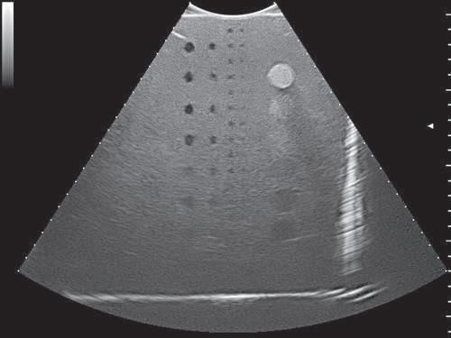
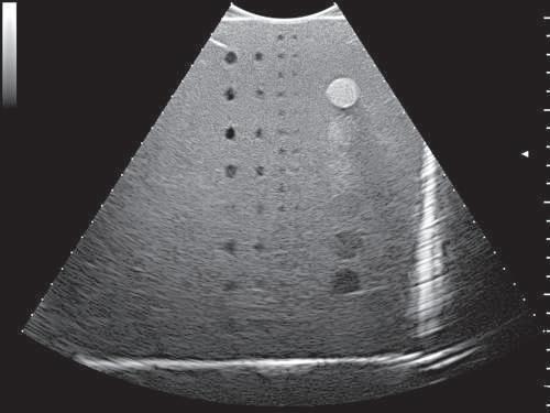
The power control modifes the voltage applied to pulse the piezoelectric crystal, thereby regulating the intensity of the sound output from the transducer. The greater the voltage spike, the larger the vibration amplitude (intensity) transmitted into tissues. Increasing the power also results in a uniform increase in the amplitude of returning echoes. The power should be set as low as possible to obtain the best resolution and prevent artifacts. This is done by choosing an appropriate transducer frequency that will penetrate to the area of interest without requiring excessive power levels. Whenever possible, the overall gain or TGC controls should be used to maximize the amplifcation of returning echoes, enabling as low a power setting as possible (Figs 1 10 and 1 11).
Overall Gain (Amplifcation) Control
The overall gain control affects the amplifcation of returning echoes and is directly responsible for overall image brightness. All ultrasound
machines have a gain control that causes uniform amplifcation of all returning echoes regardless of their depth of origin (Figs 1 12 and 1 13).
Time-Gain (Depth-Gain) Compensation Controls
The TGC controls are used to produce an image that is balanced in brightness, from near feld to far feld. Echoes returning from deeper structures are weaker than those arising from superfcial structures because of increased sound attenuation at depth. The echo return time is directly related to the depth of the refecting surface, as described previously. To selectively compensate for the weaker echoes arriving at the transducer from deeper structures, the gain is increased as the length of echo return time also increases. This compensation process is graphically represented by a TGC curve displayed on many ultrasound monitors (Fig. 1.14). The TGC curve represents the gain setting that affects specifc levels of gain throughout the image for a particular depth.
Because the near-feld echoes produce a brighter image, whereas echoes from deeper structures are more attenuated and thus darker, the operator must use the TGC controls to reduce near-feld brightness and increase the brightness of the far feld. TGC controls are usually a series of slider controls that allow the operator to intuitively adjust the TGC (see Fig. 1.7). Moving the top sliders to the left reduces near-feld brightness (overall gain at this level), whereas moving the middle and bottom sliders to the right increases image brightness accordingly. The names and appearance of the controls may vary (knobs, slider controls, or touch screen), but they all function similarly to adjust the gain at various depths. This may be represented graphically on screen, or the shape of the TGC curve may be inferred by the position of the sliders. The frst part of the TGC curve may consist of a straight portion that represents the frst few centimeters of depth in the displayed image under the near-gain control. Near gain is applied uniformly throughout this depth. The near-gain control is misnamed because it usually functions to suppress strong echoes from superfcial structures in the near feld. The TGC controls on some older ultrasound scanners are less refned, with near-feld and far-feld controls in addition to an overall gain control.
Fig. 1.10 The effects of power output on image quality. Overall gain (40%), time-gain compensation (TGC), and all other parameters are identical for both images; only the power output has been changed. A, 10% power output. B, 100% power output. The image is slightly brighter because of the increase in power. Note the better visualization of the deeper, far-feld structures. Images were made using a broadband (1 to 8 MHz) large curved-array transducer operating in the highest frequency range, using an ultrasound phantom. Power output has less effect on image brightness than overall gain.