Assistant Professor Neurology and Co-Director of the Mount Sinai Epilepsy Center, The Icahn School of Medicine at Mount Sinai, New York, USA
Rowan’s PRIMER of EEG
MADELINE C FIELDS MD
Assistant Professor Neurology and Co-Director of the Mount Sinai Epilepsy Center, The Icahn School of Medicine at Mount Sinai, New York, USA
JIYEOUN (JENNA) YOO MD
Assistant Professor Neurology, The Mount Sinai Epilepsy Center, The Icahn School of Medicine at Mount Sinai, New York, USA
Foreword
Jacqueline A French MD Professor of Neurology, New York University Comprehensive Epilepsy Center, Chief Scientific Officer, Epilepsy Foundation, New York, USA
No part of this publication may be reproduced or transmitted in any form or by any means, electronic or mechanical, including photocopying, recording, or any information storage and retrieval system, without permission in writing from the publisher. Details on how to seek permission, further information about the Publisher’s permissions policies and our arrangements with organizations such as the Copyright Clearance Center and the Copyright Licensing Agency, can be found at our website: www.elsevier.com/permissions.
This book and the individual contributions contained in it are protected under copyright by the publisher (other than as may be noted herein).
Notices
Knowledge and best practice in this field are constantly changing. As new research and experience broaden our understanding, changes in research methods, professional practices, or medical treatment may become necessary.
Practitioners and researchers must always rely on their own experience and knowledge in evaluating and using any information, methods, compounds, or experiments described herein. In using such information or methods they should be mindful of their own safety and the safety of others, including parties for whom they have a professional responsibility.
With respect to any drug or pharmaceutical products identified, readers are advised to check the most current information provided (i) on procedures featured or (ii) by the manufacturer of each product to be administered, to verify the recommended dose or formula, the method and duration of administration, and contraindications. It is the responsibility of practitioners, relying on their own experience and knowledge of their patients, to make diagnoses, to determine dosages and the best treatment for each individual patient, and to take all appropriate safety precautions.
To the fullest extent of the law, neither the publisher nor the authors, contributors, or editors, assume any liability for any injury and/or damage to persons or property as a matter of products liability, negligence or otherwise, or from any use or operation of any methods, products, instructions, or ideas contained in the material herein.
ISBN: 9780323353878
Content Strategist: Charlotta Kryhl
Content Development Specialist: Helen Leng
Project Manager: Louisa Talbott
Design: Christian Bilbow
Illustration Manager: Amy Naylor
Illustrator: Jade Myers of Matrix Inc.
Marketing Manager(s) (UK/USA): Veronica Short
Reading EEG is a skill that involves both science and art. Most of us learn by apprenticeship. If you are very lucky, you learn to read with an expert sitting in the chair next to you, helping you discover the logic and the beauty of the squiggles on the page. Slowly, these squiggles that initially seem incomprehensible begin to emerge as an unfolding story. Through interpretation of the EEG (if done correctly), much is revealed about the person being tested. With time, one learns to uncover hints and clues, like a detective, that lead to a correct interpretation.
I was fortunate enough to have had A. James Rowan sitting next to me as I learned to read EEG. Now with his primer, updated by Marcuse, Fields and Yoo, those learning to read for the first time can benefit from a simple, easy to follow, pragmatic guide that is perfect for carrying with you to have at your side as you learn to become comfortable with the EEG. Essential information is easy to find, and the pictures and diagrams
beautifully illustrate the normal and abnormal EEG. The chapter on the technical aspects of the EEG is clear, simple and easy to follow. The illustrations of artifact have been carefully chosen, as have the normal variants and pathological epileptiform and nonepileptiform abnormalities. Each chapter provides just enough material to be helpful but not overwhelming, and there is a reference section for those seeking more indepth information. The book will also be extremely useful to teachers of EEG, and I for one will be using the illustrations to train young encephalographers.
According to the dictionary, a primer is a book that “provides instruction in the rudiments or basic skills of a branch of knowledge”. Those who master this primer will be well on their way to learning the art of EEG interpretation.
Jacqueline A French MD
Dedication
We dedicate this book to our patients (and yours as well): past, present, and future.
Preface to the second edition
“If I keep on saying to myself that I cannot do a certain thing, it is possible that I may end by really becoming incapable of doing it. On the contrary, if I have the belief that I can do it, I shall surely acquire the capacity to do it even if I may not have it at the beginning.” – Mahatma Gandhi
With this book, we seek to lay the art of reading EEGs at your feet. We have built upon the structure of the first edition. We have added a chapter entitled The normal EEG from neonates to adolescents. All pictures of EEGs have been replaced, to give the readers up-to-date examples of normal and abnormal findings. In Chapter 5 we describe the typical EEG findings in all seizure types, electroclinical syndromes and other epilepsies as listed by the International League Against Epilepsy (ILAE).
Learning to understand an EEG is wonderful, and reporting those findings with standard nomenclature ensures that we all mean the same thing when we use the same word. This edition uses the 10-10 system of electrode placement and the nomenclature put forth by the American Clinical Neurophysiology Society (ACNS).
If you are a medical student with no intention of becoming a neurologist, we believe this primer will serve you well in understanding the EEG reports of both your outpatients and inpatients. If you are a neurologist or a neurology resident, we have included details which are useful to have at one’s fingertips and easily forgotten (e.g., the meaning of subclinical rhythmic electroencephalographic discharges of adults).
As a companion to the print book, this edition has an online version, which includes a quiz for each chapter. Be warned, these questions are challenging. The answers are detailed and meant to help you integrate what you are learning of EEG with clinical care and clinical decisionmaking. Perhaps most importantly, we have created a video library of
seizures. These can be watched with our annotations describing the seizure semiology and the electrographic findings, or you can choose to watch the seizures without the annotations to test your developing skill. We will be adding to the video library continually to build on your knowledge.
Learning the skill of electroencephalography may be challenging, it may be daunting, and it may not give us all the answers. However, it is a relatively inexpensive window into the workings of the brain, which often provides very valuable information for diagnosis, prognosis, and management of our patients.
We hope this primer will serve to increase your enthusiasm and dedication to the study of the brain, as this inquiry continues to nourish us as clinicians, teachers and researchers.
Lara V Marcuse MD (r)
Madeline C Fields MD (c)
Jiyeoun (Jenna) Yoo MD (l)
1 Origin and technical aspects of the EEG
ORIGIN OF THE EEG
The EEG records electrical activity from the cerebral cortex. Inasmuch as electrocortical activity is measured in microvolts (µV), it must be amplified by a factor of 1,000,000 in order to be displayed on a computer screen. Most of what we record is felt to originate from neurons, and there are a number of possible sources including action potentials, post-synaptic potentials (PSPs), and chronic neuronal depolarization. Action potentials induce a brief (10 ms or less) local current in the axon with a very limited potential field. This makes them unlikely candidates. PSPs are considerably longer (50–200 ms), have a much greater field, and thus are more likely to be the primary generators of the EEG. Longterm depolarization of neurons or even glia could also play a role and produce EEG changes.
In the normal brain an action potential travels down the axon to the nerve terminal, where a neurotransmitter is released. However, it is the synaptic potentials that are the most important source for the electroencephalogram. The resting membrane potential (electrochemical equilibrium) is typically –70 mV on the inside. At the post-synaptic membrane the neurotransmitter produces a change in membrane conductance and transmembrane potential. If the signal has an excitatory effect on the
neuron it leads to a local reduction of the transmembrane potential (depolarization) and is called an excitatory post-synaptic potential (EPSP), typically located in the dendrites. Note that during an EPSP the inside of the neuronal membrane becomes more positive while the extracellular matrix becomes more negative. Inhibitory post-synaptic potentials (IPSPs) result in local hyperpolarization typically located on the cell body of the neuron. The combination of EPSPs and IPSPs induces currents that flow within and around the neuron with a potential field sufficient to be recorded on the scalp. The EEG is essentially measuring these voltage changes in the extracellular matrix. It turns out that the typical duration of a PSP, 100 ms, is similar to the duration of the average alpha wave. The posterior dominant rhythm (PDR), consisting of sinusoidal or rhythmic alpha waves, is the basic rhythmic frequency of the normal awake adult brain.
It is easy to understand how complex neuronal electrical activity generates irregular EEG signals that translate into seemingly random and ever-changing EEG waves. Less obvious is the physiological explanation of the rhythmic character of certain EEG patterns seen both in sleep and wakefulness. The mechanisms underlying EEG rhythmicity, although not completely understood, are mediated through two main processes. The first is the interaction between cortex and thalamus. The
activity of thalamic pacemaker cells leads to rhythmic cortical activation. For example, the cells in the nucleus reticularis of the thalamus have the pacing properties responsible for the generation of sleep spindles. The second is based on the functional properties of large neuronal networks in the cortex that have an intrinsic capacity for rhythmicity. The result of both mechanisms is the creation of recognizable EEG patterns, varying in different areas of neocortex that allow us to make sense of the complex world of brain waves.
TECHNICAL CONSIDERATIONS
The essence of electroencephalography is the amplification of tiny currents into a graphic representation that can be interpreted. Of course, extracerebral potentials are likewise amplified (movements and the like), and these are many times the amplitude of electrocortical potentials. Thus, unless understood and corrected for, such interference or artifacts obscure the underlying EEG. Like the archeologist, the epileptologist seeks to fully understand artifacts in order to discern the truth. Later, we will discuss artifacts in detail and illustrate clearly their many guises. At this point we will consider the technical factors that are indispensable in obtaining an interpretable record.
ELECTRODES
Electrodes are simply the means by which the electrocortical potentials are conducted to the amplification apparatus. Essentially, standard EEG electrodes are small, non-reactive metal discs or cups applied to the scalp with a conductive paste. Several types of metals are used including gold, silver/silver chloride, tin, and platinum. Electrode contact must be firm in order to ensure low impedance (resistance to current flow), thus minimizing both electrode and environmental artifacts.
For long-term monitoring, especially if the patient is mobile, cup electrodes are affixed with collodion (a sort of glue), and a conductive gel is inserted between electrode and scalp through a small hole in the electrode itself. This procedure maintains recording integrity over prolonged periods.
Other types of electrodes are available including plastic, as well as needle electrodes. In fact, new plastic electrodes are MRI compatible. Needle electrodes, which in the past were often used in ICUs, have been redeveloped and consist of a painless (really!) subdermal electrode.
ELECTRODE PLACEMENT
Electrode placement is standardized in the United States and indeed in most other nations. This allows EEGs performed in one laboratory to be interpreted in another. The general problem is to record activity from various parts of the cerebral cortex in a logical, interpretable manner. Thanks to Dr. Herbert Jasper, a renowned electroencephalographer at the Montreal Neurological Institute, we have a logical, generally accepted system of electrode placement: the 10-20 International System of Electrode Placement (Figure 1-1). The numbering has been slightly modified since the last edition to a 10-10 system (Figure 1-2). The system was modified so that if additional electrodes are to be placed on the scalp, there is a logical numbering system with which to do so.
Both the 10-10 and the 10-20 system depend on accurate measurements of the skull, utilizing several distinctive landmarks. Essentially, a measurement of the skull is taken in three planes – sagittal, coronal, and horizontal. The summation of all the electrodes in any given plane will equal 100%. Electrodes designated with odd numbers are on the left; those with even numbers are on the right. Standard electrode designations and placement should be memorized during the student’s first day of his or her elective (Table 1-1).
Figure 1-1 10-20 system. A single-plane projection of the head showing all standard positions and the locations of the Rolandic and Sylvian fissures. The outer circle was drawn at the level of the nasion and inion. The inner circle represents the temporal line of electrodes.
Origin and technical aspects of the EEG
Figure 1-2 10-10 system. The 10-20 system has been modified to standardize a method for adding more electrodes.
Table 1-1 Standard electrode designations
Left Right Electrode
Parasagittal/supra-sylvian electrodes
Fp1 Fp2
Frontopolar, located on the forehead – postscripted numbers are different than other electrodes in this sagittal line (3,4)
F3 F4 Mid-frontal
C3 C4 Central – roughly over the central sulcus
P3 P4 Parietal
O1 O2
Occipital-postscripted numbers are different from other electrodes in this sagittal line (3,4)
Fz, Cz, Pz Midline electrodes: Frontal, central and parietal.
A1 A2 Earlobe electrodes. Often used as reference electrodes from contralateral side. Of note, they record ipsilateral mid-temporal activity.
LLC RUC Left lower canthus/right upper canthus (placed on the lower and upper outer corners of the eyes). These electrodes are used to detect eye movements and can help distinguish eye movements from brain activity. Sometimes designated LOC, ROC.
How to measure for electrode placement
Sagittal plane: The sagittal measurement starts at the nasion (the depression at the top of the nose) over the top the head to the inion (the prominence in the midline at the base of the occiput). With a red wax pencil, mark the point above the nasion that is 10% of the total measurement (Fpz) and the point above the inion that also is 10% of the total (Oz). These locations are used as coordinates to help identify the other designated electrode destinations. Divide and mark the remaining 80% into four segments, each 20% of the total measurement. The first 20% point is Fz, the second Cz and the third Pz – the
midline electrodes (z = zero). The final 20% is the distance between Pz and your point 10% above the inion (Oz). Thus, the total is 100% (Figure 1-3A).
Coronal plane: The coronal plane extends from the point anterior to the tragus (the cartilaginous protrusion at the front of the external ear) to the same point on the opposite side, making sure that the tape measure traverses the Cz point on the sagittal measurement. The intersection of the halfway (50%) points of the sagittal and coronal measurements is the location of the vertex and thus the Cz electrode. The first 10% points up from the tragus define T7 and T8, the mid-temporal electrodes. The next 20% points then define C3 and C4, the central
Origin and technical aspects of the EEG
electrodes. The remaining 20% segments represent the distance from C3 to Cz and Cz to C4 (Figure 1-3B).
Horizontal plane: The trickiest measurements are in the horizontal plane. The horizontal plane is generated with a measurement from Fpz to T7 to Oz on the left and from Fpz to T8 to Oz on the right. Fp1 and Fp2 are placed on either side of Fpz, both a distance of 5% of the total horizontal circumference from Fpz. Similarly, O1 and O2 are placed at a 5% distance of the total horizontal circumference from Oz. The distances from Fp1 to F7 to T7 to P7 to O1 on the left and from Fp2 to F8 to T8 to P8 to O2 on the right are all 10% of the total horizontal circumference (Figure 1-3C).
Figure 1-3 Measurements in the 10-10 system in the (A) sagittal, (B) coronal, and (C) horizontal plane. (A) Lateral view of the skull to show the method of measurement from the nasion to inion at the mid-line. Fp is the frontal pole position, F is the frontal line of electrodes, C is the central line, P is the parietal line, and O is the occipital line. Percentages indicate proportions of the total measurement from the nasion to the inion. The central line is 50% of this distance. (B) Frontal view of the skull showing the coronal measurements.
Finally, F3 and F4 are defined by the halfway points between F7 and Fz on the left and F8 and Fz on the right. Similarly, P3 and P4 are defined by the halfway points between P7 and Pz on the left and P8 and Pz on the right.
An observation: The F7 and F8 electrodes are probably placed too high for optimal definition of anterior temporal activity. Likewise, the P7 and P8 electrodes are probably too high for good definition of posterior temporal activity. Thus, it is possible to logically place additional electrodes (F9/F10, T9/T10, and P9/P10), which are placed 10% inferior to the standard (F7/8, T7/8, P7/8, respectively) electrodes. In some laboratories, these additional electrodes are routinely used.
In the 10-10 system, there are remaining electrode positions in the 10% intermediate lines between the existing standard coronal and sagittal lines. Best to look at Figure 1-2 while reading the next several sentences. Coronally, these electrode positions are named by combining the designation of the coronal lines anterior and posterior. For example, the coronal line between the parietal (P) and occipital (O) chain is designated PO. The only exception is in the first intermediate coronal line, which is named AF (anterior frontal) rather than FpF or FF. In the sagittal line, the same postscript numbers are used; for example, AF3, F3, FC3, C3, CP3, P3, and PO3. From the midline moving laterally the postscript begins at z followed by the numbers 1, 3, 5, 7, 9 on the left and 2, 4, 6, 8, 10 on the right. We now have the 10-10 system where each letter appears on only one coronal line and each postscripted number on a sagittal line (except for Fp1/Fp2 and O1/O2). The 10-10 system locates each electrode at the intersection of a specific coronal (identified by the letter) and sagittal (identified by the number) line.
While the 10-10 system may sound ever so slightly complicated, in practice it is quite easily carried out. Nonetheless, there is nothing like actually measuring and placing the electrodes yourself under the guidance of an experienced EEG technologist. We recommend that all
1-3, cont’d
(C) Superior view with cross-section of the skull through the temporal line of electrodes.
Figure
residents perform at least two to three supervised EEGs during their EEG rotations. Fellows should do more until they are confident in their ability to measure accurately and apply electrodes properly.
POTENTIAL FIELDS
Before discussing how we display the electrical information recorded by the electrodes, the reader should understand the concept of the potential field. The summation of IPSPs and EPSPs in a neuronal net creates
Origin and technical aspects of the
EEG
electrical currents that flow in and around the cells. The flow of current creates a field that spreads out from the origin of an electrical event (such as a spike or slow wave), much the same as the concentric rings created on a glassy pond when one tosses a pebble onto its surface. Potential fields are usually oval in shape and may be quite restricted or very widespread. The field’s effect diminishes as the distance from the source increases. This means that events producing maximal voltage on a particular electrode will affect adjacent electrodes as well, but to a lesser extent as the potential wanes from the point of origin (Figure 1-4).
Figure 1-4 A potential field. (A) The figure illustrates a maximum negative potential of -100 µV at F8. The field spreads to involve T8 at a lower potential of –70 µV and then to Fp2 and P8 at –30 µV. The background averages –20 µV. (B) Another way to depict the same data. Note the steep rise from Fp2 to F8, declining successively to T8 and P8.
AMPLIFICATION
Easiest to understand is the simple amplifier. Input from a single active electrode is conducted to the amplifier and compared with ground (earth). Thus, the output consists of the potential difference between the active electrode and ground. Electrocortical potentials, as well as other environmental potentials affecting the electrode (e.g., 60 Hz interference), are displayed in the output. In differential amplification, signals from two active leads are conducted to the amplifier, thus measuring the potential difference between the two (Figure 1-5). In this case, any signal that affects both inputs identically (say 60 Hz) will result in no potential difference and thus will not be displayed or be much reduced. This phenomenon is termed in-phase cancellation.
We are now in a position to consider methods of recording electrocortical potentials so that we can make sense of them. Recalling that amplifiers record potential difference between two incoming signals, we can record the potential difference between two electrodes on the scalp (bipolar recording). On the other hand, we can record the potential difference between a scalp electrode and another point (the reference) that, ideally, is unaffected by cerebral potentials or other interference (referential recording). Unfortunately, it is virtually impossible to achieve this ideal, but certain references (e.g., the ears) are quite serviceable. These two types of recording, along with their advantages and disadvantages, are discussed below.
BIPOLAR RECORDING
Bipolar recordings electronically link successive electrodes (known as a chain or line). The voltage at one electrode is compared with the voltage affecting adjacent electrodes (potential difference). Each amplifier has two inputs, I and II. By convention, the rules for understanding the display are:
Figure 1-5 (A) Simple amplifier. Input from each active electrode is compared with ground. (B) Differential amplifier. Here, potential difference is measured between two active electrodes.
If input I becomes negative with respect to input II, there is an upward deflection.
If input II becomes negative with respect to input I, there is a downward deflection.
Contrary to our well-used Cartesian coordinate system, the convention in neurophysiology is that an upward deflection is negative and a downward deflection is positive.
In the simplest example, consider a spike with a very limited potential field involving only T8 (Figure 1-6). The electrode pairs (or derivations) in this case are F8–T8 and T8–P8. F8–T8 is Channel 1, and T8–P8 is Channel 2. In Channel 1 T8 is in input II, and in Channel 2 T8 is in input I. The voltage at T8 (–100 µV) is compared with the background activity at F8 and P8 (–20 µV). Therefore, in this example:
In this case, the adjacent channels containing the T8 electrode record the same potential but in opposite directions. This creates the phase reversal. Most spike discharges at the surface are negative in sign, and negative phase reversals resemble two sharp points touching or nearly touching. Channels 1 and 2 are displaying the same potential but with opposite deflections. Again, this is phase reversal – the localization principle of bipolar recording.
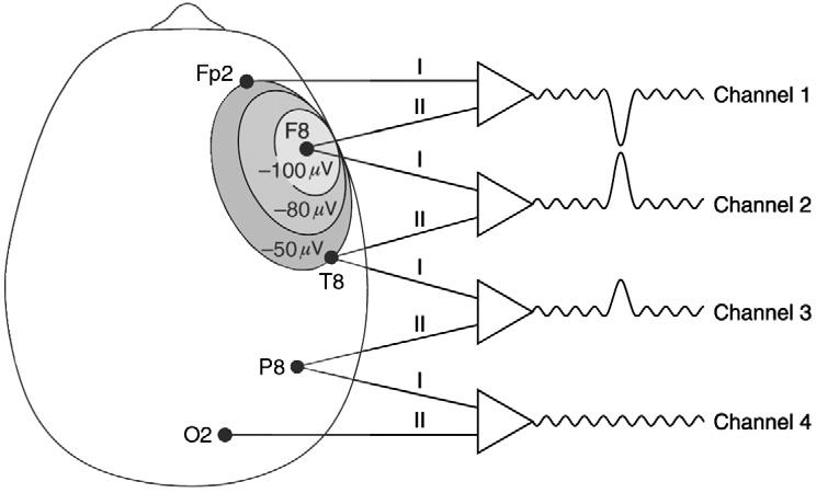
Let us now analyze the display when a spike at F8 has a wider potential field that also affects Fp2 and T8 (Figure 1-7A). In Channel 1, the voltage at Fp2 (–50 µV) is compared with the voltage at F8 (–100 µV). In Channel 2, the voltage at F8 (–100 µV) is compared with the voltage at T8 (–50 µV). In Channel 3, the voltage at T8 (–50 µV) is compared
Origin and technical aspects of the EEG
Figure 1-6 Principle of bipolar localization. The figure depicts a spike discharge of –100 µV at T8. The potential is conducted to input II in the first amplifier and to input I in the second amplifier. Other electrodes are not affected by the event. The result is known as a phase reversal.
to the voltage P8, which is unaffected by the spike at F8 but is recording the background activity (–20 µV). In Channel 4, the voltage at P8 is compared with O2, both unaffected by the F8 spike. Thus, there is no potential difference and no deflection.
Figure 1-7 (A) Phase reversal in longitudinal bipolar montage. Here, a spike of –100 µV at F8 spreads to involve Fp2 and T8, each at –50 µV. The potential difference between F8 and the other two electrodes is 50 µV. The display demonstrates a phase reversal at F8 (Channels 1 and 2) with representation of the spike in Channel 3 (the potential difference between T8 and P8 is –30 µV). (B) Referential montage. The same spike displayed in a referential montage. In a referential montage, each electrode is compared to a reference electrode. The potential at the active electrode is conducted to input I of each amplifier. The reference electrode is conducted to input II. The amplitude of the displayed spike is proportional to the voltage at each active electrode.
Other channels (e.g., F4–C4 and C4–P4) may be affected by the declining potential field generated at F8. Thus, phase reversals at lower amplitude would be recorded at these sites. Note that these considerations apply to any potential at any point on the scalp.
REFERENTIAL RECORDING
In referential recording the amplifiers are not linked as in bipolar recording. Signals from each of the scalp electrodes are conducted to input I of the associated amplifier, while signals from the reference are
conducted to input II. Thus, in referential recording, we record the potential difference between a particular scalp electrode and a referential electrode. Reference montages produce a higher amplitude EEG recording because of the longer interelectrode distances. Theoretically, the reference can be located anywhere, but there are practical considerations. A reference placed at any distant point will be contaminated with ambient electrical noise, 60 Hz artifact (50 Hz in Europe). A reference placed on, say, the shoulder or chest would also pick up high-voltage EKG artifact. Interference from an EKG would render the EEG
unreadable. The ears are relatively free from both these artifacts, although it must be said that EKG is sometimes a contaminant at the ear electrodes. Moreover, due to the proximity of the ears to the midtemporal lobes, the ears do pick up cerebral activity.
Now, utilizing the ears as a contralateral reference, let us compare the voltage of an event occurring at F8 with that at a contralateral ear reference, A1 (Figure 1-7B). In this example we will assume that A1 is recording the same as the background at –20 µV. Here we have a spike discharge with an amplitude of –100 µV at F8. The potential field of the spike spreads to Fp2 and T8 with an amplitude of –50 µV. Beyond these points there is no representation of the field associated with the spike.
In referential recording, the localization principle is amplitude. That is, the electrode recording the greatest amplitude of the wave in question, in this case a spike at F8, defines the focus.
References other than the ears are also in common use. One is the vertex (Cz), often used in a referential montage to complement the ear reference. The astute reader will recognize that the vertex resides in a sea of cerebral activity. Thus, the background of the EEG recorded by the vertex electrode will be input II of all channels. As long as this is recognized, one is able to determine the location of a waveform that stands out from the background (e.g., a spike or delta wave).
Origin and technical aspects of the EEG 1
A note on ear and vertex referential recording: A recorded event (spike, slow wave) is best represented when the reference is distant from the exploring electrode. Considering the ipsilateral ear reference (A1 or A2), the ear is close to the midtemporal electrodes T7 or T8. When examining a spike at T7, the ipsilateral ear reference (A1) is not an appropriate choice, as the potentials at T7 and A1 are very similar. A vertex reference or a contralateral ear reference (A2) is more appropriate for the examination of that T7 spike. Similarly, a spike that is maximal at C3 will be ill served by placing it in a reference montage using the Cz electrode, as the reference and the active electrode are too close together. For a C3 spike, either ear electrode would be an appropriate reference. The reference chosen for a particular spike should be as distant as possible from that spike.
A widely used reference is the common average reference. In this scheme, the voltage of an event occurring under a particular electrode (input I) is compared with the average voltage recorded by all the electrodes on the scalp (input II). This creates a situation in which a focal spike discharge, maximal at T8, will result in an upward deflection at T8 as T8 will be more electronegative than the average reference. Neighboring electrodes involved in the field, for example at F8, will have upward deflections as well, but these will be lower in amplitude. Note that the upward deflections thus recorded define the potential field of the event. Electrodes not involved in the negative spike discharge at T8 will be relatively electropositive compared with the average reference and thus will have a downward deflection (Figure 1-8).
We now present the paradox of bipolar recording and stress how important it is to use the various montages in a complementarily fashion. The paradox is a result of the previously mentioned in-phase cancellation – that is, potentials that are equal in the two inputs of an amplifier are isoelectric in the display. In other words, there is no potential
difference! The unwary, when examining Channels 2 and 3 of Figure 1-9A, might conclude that little if anything is occurring at F8, T8, and P8. On the other hand, when one looks at the same situation with a referential recording, it becomes clear that the maximum abnormality underlies those very electrodes (Figure 1-9B).
MONTAGE SELECTION
Montage refers to the pattern of systematic linkage of the scalp electrodes designed to obtain a logical display of the electrical activity. Unlike the 10-10 system of electrode placement described earlier, there is no international standard of montages to be used in EEG laboratories. Certain montages, however, are in widespread use. In bipolar recording the longitudinal arrangement is perhaps the most popular (known in the trade as the “double banana,” and by some as the Queen Square
Figure 1-8 The common average reference. Recording of a spike discharge at T8 of –100 µV. The reference (going into input II at each channel) is the common average voltage, which in this case is –20 µV. In Channels 2, 3, and 4 the amplitude is proportional to the recorded voltage at each electrode. The downward deflection in channels 1 and 5 is due to the fact that Fp2 and O2 are relatively electropositive (–10 µV) compared with the average voltage (–20 µV).
montage) (Figure 1-10A). Note: arrows are often used in North America for convenience: the tail of the arrow indicates input I; the point of the arrow input II.
Adjacent electrodes are connected from front to back, including the temporal (lateral) chain and the parasagittal (supra-sylvian) chain. The EEG is displayed in various ways. In this example, the four channels of the temporal chain on one side are followed by the temporal channels on the opposite side. Similarly, the four channels of the parasagittal chain also alternate. In North America, the left side is written out first followed by the right. In Europe the opposite is the case. Some laboratories write out the eight channels of left-sided electrodes followed by the right-sided electrodes. Still others prefer alternating homologous channels, for example, Fp1 → F7; Fp2 → F8, and so on. Overall, the latter tends to be a bit more confusing – but electroencephalographers experienced with a particular electrode arrangement have no difficulty.
Origin and technical aspects of the EEG
1
Figure 1-9 The paradox of bipolar recording. (A) Representation of a –100 µV spike that affects F8, T8, and P8 equally. Inasmuch as there is no potential difference between F8–T8 and T8–P8, the spike is not recorded in Channels 2 and 3 and gives the impression that there is no abnormality at T8. (B) Same discharge in referential recording. Note equal deflection in Channels 2, 3, and 4. The true picture is thus displayed.
A second popular arrangement is the transverse bipolar montage. This links adjacent electrodes in transverse chains, starting anteriorly and progressing posteriorly. Each chain starts with the left side and progresses to the right (i.e., F7 → F3 → Fz → F4 → F8). The transverse montage is particularly well suited to record abnormalities occurring at or near the vertex (e.g., midline spikes) (Figure 1-10B). One additional bipolar montage comes to mind: the circumferential montage. As the name implies, the circumferential montage encircles the head and is particularly useful for examining spikes and sharp waves, which
occur at the end of the longitudinal bipolar chain: Fp1, Fp2, O1 or O2 (Figures 1-10C and 1-11).
With respect to referential recording, the recording is usually displayed in both A-P and transverse arrangements, reprising commonly used bipolar montages. A variety of other montages are employed at the discretion of the individual electroencephalographer. The idea, in short, is to highlight certain areas of interest in the best possible way. If the student is familiar with the 10-10 system and is apprised of the montage, he or she should have no difficulty in interpreting the record.
In the era of digital EEG, specific montage selection by the technologist is not as critical as it was in the analog days. All recording is actually done referentially. The software allows display of recorded potentials in any desired montage. Thus, the technician and reader can now easily switch from one montage to another to examine the characteristics of a particular phenomenon. A low-amplitude temporal spike during bipolar recording can rapidly be inspected on a referential montage with the flick of the computer mouse.
Figure 1-10 (A) A typical longitudinal bipolar montage. The numbers refer to channels, reflecting voltage difference between two electrodes. Both temporal and supra-sylvian chains alternate from left to right. The arrows represent the inputs to each amplifier. The tail is in input I and the arrow is in input II. (B) A transverse bipolar montage. The chains run from left to right, beginning anteriorly and proceeding posteriorly. Note that the midline electrodes are incorporated into the second, third, and fourth chains, thus allowing good representation of midline events.
In summary, the technologist may record an EEG in a set sequence of montages but the reviewing electroencephalographer can review the EEG in any montage desired. Furthermore, a given page or discharge can be examined in a variety of montages to help understand its meaning.
Much as we would circle a complex sculpture in a museum, we circle an EEG wave by using different montages. Remember, the central idea is to maximize the opportunity to display an abnormality for optimal recognition.
Figure 1-10, cont’d
(C) Circumferential bipolar montage.
OVERVIEW OF ELECTRONICS
We often say that the EEG display can be manipulated at will and made to demonstrate a severe abnormality or to show a normal pattern. This manipulation refers to changing the electronic circuitry with the press of a button in order to alter sensitivity, filtration, and timebase.
Origin and technical aspects of the EEG 1
Clearly, some order was required so that EEGs obtained in one laboratory are easily interpretable at another. For many years nearly all laboratories in North America, and indeed in many laboratories throughout the world, have used similar electronic settings for routine work. Following is a brief discussion of the most important recording parameters.
Calibration
Calibration is a way to accurately measure EEG potentials by administrating a standard signal through each amplifier. Once this is performed, the voltage of an EEG potential is compared against this known voltage. Calibration is currently built into the software of most digital EEG systems and is performed automatically. Additionally, an impedance check should appear at the start of every recording. The impedance check is a way of establishing the integrity of each electrode. Impedances should not exceed 5 kohms.
Display
In most North American and many European laboratories the standard display timebase is 30 mm/sec with 10 seconds of EEG per display. There is nothing magic about the number – in fact, some laboratories (particularly in Europe) prefer a timebase of 15 mm/sec. The appearance of the EEG is considerably altered in the latter case (i.e., the alpha rhythm at 30 mm/sec looks like rhythmic beta activity at 15 mm/sec). The important point is that the reader knows what timebase is selected. It should be said that there are instances when use of a shorter timebase is quite useful (e.g., in the identification of periodicity, or even rhythmicity of a particular phenomenon [e.g., in ICUs or for neonatal EEGs]). Likewise, increasing the timebase to, say, 60 mm/sec may allow one to analyze more accurately wave configuration, particularly when a phenomenon is “crowded” as in grouped spikes.
Figure 1-11 Occipital spike. Spike discharges at the “end of chain (Fp1, Fp2, O1, O2)” can be easy to miss in the standard longitudinal bipolar montage. Here, a right occipital (O2) spike discharge is displayed at –100 µV. (A) In a standard longitudinal bipolar montage, the deflection is always downward. (B) The discharge can be confirmed by placing it in a circumferential bipolar montage. Phase reversal at O2 confirms the spike maximum at this location.
Sensitivity
The sensitivity of each channel refers to the amplitude of the display produced by the received signal. The measurement is expressed in voltage per deflection. Standard sensitivity is 7 µV/mm.
Sensitivity may be altered for any particular channel depending on the specific need. For example, the sensitivity of a channel recording the EKG would have to be decreased due to the much higher voltage of this signal (measured in millivolts). In general, the sensitivity of all channels recording the EEG may be changed simultaneously by a stepped gain control. For example, one might wish to increase sensitivity in situations where the general voltage of the EEG is low. Similarly, some EEG phenomena reach very high voltages (e.g., generalized spike-wave discharges), requiring a decrease in sensitivity (15 µV/mm) in order to properly analyze the waveforms. Please note, raising the gain from, for example, 7 µV to 15 µV is the same thing as lowering the sensitivity, and the EEG will appear lower in amplitude.
High-frequency filters (HFFs) or low pass filters
This circuit attenuates undesirable high frequencies (e.g., muscle action potentials) and passes low frequencies (Figure 1-12A). In an HFF circuit, the input signal is placed across the combination of a resistor and a
Figure 1-12 (A) High-frequency filter. In a high-frequency filter, the output voltage for high frequencies is lower than the input voltage for high frequencies. In the log–log graph, frequencies below the cutoff are unchanged while frequencies above the cutoff are attenuated. (B) Low-frequency filter. In a low-frequency filter, the output voltage for low frequencies is lower than the input voltage for low frequencies. In the log–log graph frequencies above the cutoffs are unchanged while frequencies below the cutoff are attenuated. (Adapted with permission from Lippincott Williams & Wilkins/Wolters Kluwer Health: Schomer, Lopes da Silva, Niedermeyer’s Electroencephalography, 2010.)
Origin and technical aspects of the EEG 1
capacitor in series and the output signal is measured across the capacitor alone (Figure 1-12A). At high frequencies, the impedance of any capacitor is low. Measuring output across the capacitor with a high frequency will be essentially zero, as the voltage does not change, so the potential difference is zero. The standard HF setting is 70 Hz. Other standard settings are 35 Hz and 15 Hz, the latter severely attenuating a broad range of high frequencies. As a practical matter, recording at a HFF setting of 15 Hz should not be employed save in rare and unusual circumstances. An unwanted consequence would be a marked attenuation of spike potentials. Unfortunately, the authors have inspected EEGs from outside sources in which an HFF setting of 15 Hz was used throughout. Such records look “clean” but fail to convey needed information. Don’t do it.
Low-frequency filters (LFFs) or high-pass filters
In an LFF, there is marked attenuation of slow potentials below the cutoff frequency (such as those caused by sweat artifact, respirations, and tongue movement), with little effect on rapid potentials such as spikes or muscle artifacts. In an LFF circuit, the input signal is placed across the combination of a capacitor and a resistor in series and the output signal is measured across the resistor alone (Figure 1-12B). The impedance of any capacitor is very high at low frequencies. In this circuit arrangement, low-frequency input signals are essentially blocked. At higher frequencies, the impedance at the capacitor is low and the signal is measured across the resistor essentially unchanged from the input. The LFF is typically set at 1 Hz.
Notch filter
In addition, a notch filter setting of 60 Hz (US) or 50 Hz (Europe) is usually employed, selectively reducing environmental interference.
NOTES ON RECORDING THE EEG
Many special problems confront the technologist in his or her efforts to obtain an EEG that can be interpreted successfully by the electroencephalographer. We emphasize that the electroencephalographer is totally dependent on the quality of the recording – that is, regardless of the expertise of the reader, he or she is unable to use that expertise in the face of a technically inadequate tracing. The ability to properly place electrodes in conformity with the 10-10 International System (including, importantly, accurate measurements of electrode location) is critical if one is to compare electrical activity between the two hemispheres with accuracy. If epilepsy is suspected, the technologist should attempt to record drowsiness and sleep if possible. Moreover, because focal epileptiform activity is often activated by the interface between wake and drowsiness, the technologist should gently alert the drowsy patient on several occasions in an attempt to provoke spikes. Similarly, if a patient is sleeping at the onset of the test, he or she should be aroused after some minutes of recording. This ensures that a relative waking record is obtained. Unfortunately, sleep may obscure background abnormalities
that are only evident when the patient is awake – a circumstance sometimes encountered in patients with dementia.
ARTIFACTS
Recognition of artifacts is one of the vexing and strangely satisfying aspects of EEG interpretation, as well as one of the most important. As a beginner, you may find the differentiation of artifacts from physiological phenomena quite difficult. A distinguishing characteristic of the experienced electroencephalographer is the ability reliably to recognize artifacts. For the most part the reader will soon master artifact recognition, particularly after understanding their characteristics and referring to the mini-atlas, and should not be too daunted by the seeming impossibility of this task!
Artifacts come in many different forms and have diverse causes. The major underlying problem is the enormous amplification required to record brain waves. As a result, amplified non-cerebral potentials – for example vigorous movements by the patient producing random excursions of the electrode leads – may render the EEG uninterpretable. Specific artifacts are detailed in Figures 1-13–1-30.
Figure 1-14 EKG artifact. Diffuse sharp potentials (arrows) coincident with the EKG. The artifact is particularly prominent in channels connected to the ears. It also may be diffuse. If there is no EKG monitor, and if the patient has atrial fibrillation or frequent premature contractions, the artifact may be confounding, be inconsistent, and masquerade as spike discharges. Look for phase relationships that do not comport with those of true spikes. EKG artifact is particularly prominent in the obese and those with hypertension.