Cambridge University Press is part of Cambridge University Press & Assessment, a department of the University of Cambridge.
We share the University’s mission to contribute to society through the pursuit of education, learning and research at the highest international levels of excellence.
www.cambridge.org
Information on this title: www.cambridge.org/9781009401760
This work is in copyright. It is subject to statutory exceptions and to the provisions of relevant licensing agreements; with the exception of the Creative Commons version the link for which is provided below, no reproduction of any part of this work may take place without the written permission of Cambridge University Press.
An online version of this work is published at doi.org/10.1017/9781009401807 under a Creative Commons Open Access license CC-BY-NC-ND 4.0 which permits re-use, distribution and reproduction in any medium for non-commercial purposes providing appropriate credit to the original work is given. You may not distribute derivative works without permission. To view a copy of this license, visit https://creativecommons.org/licenses/by-nc-nd/4.0
All versions of this work may contain content reproduced under license from third parties. Permission to reproduce this third-party content must be obtained from these third-parties directly.
When citing this work, please include a reference to the DOI 10.1017/9781009401807
First published 1984
First paperback printing 1985
Reprinted 1987, 1989, 1992, 1995, 1998 Reissued as OA 2023
A catalogue record for this publication is available from the British Library
ISBN 978-1-009-40176-0 Hardback
ISBN 978-1-009-40179-1 Paperback
Cambridge University Press & Assessment has no responsibility for the persistence or accuracy of URLs for external or third-party internet websites referred to in this publication and does not guarantee that any content on such websites is, or will remain, accurate or appropriate.
5.3
5.3.1
5.7.2
5.7.3
5.7.4
5.7.5
5.9
5.9.1
6.1
7.1
7.4.1
7.5
7.5.1
7.8
7.9
7.10
8.4
8.4.1
1
Introduction
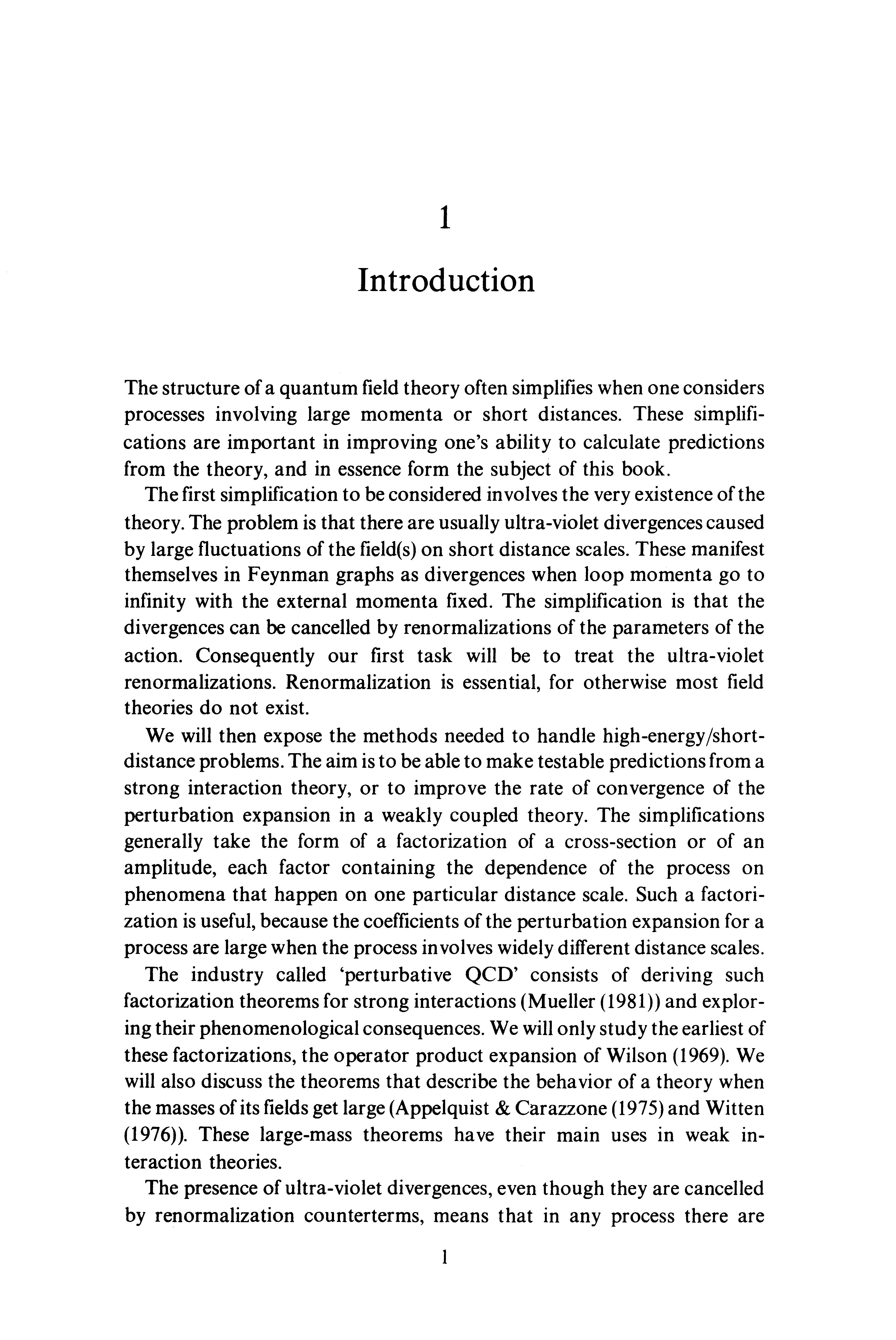
The structure of a quantum field theory often simplifies when one considers processes involving large momenta or short distances. These simplifications are important in improving one's ability to calculate predictions from the theory, and in essence form the subject of this book.
The first simplification to be considered involves the very existence of the theory. The problem is that there are usually ultra-violet divergences caused by large fluctuations of the field(s) on short distance scales. These manifest themselves in Feynman graphs as divergences when loop momenta go to infinity with the external momenta fixed. The simplification is that the divergences can be cancelled by renormalizations of the parameters of the action. Consequently our first task will be to treat the ultra-violet renormalizations. Renormalization is essential, for otherwise most field theories do not exist.
We will then expose the methods needed to handle high-energy/shortdistance problems. The aim is to be able to make testable predictions from a strong interaction theory, or to improve the rate of convergence of the perturbation expansion in a weakly coupled theory. The simplifications generally take the form of a factorization of a cross-section or of an amplitude, each factor containing the dependence of the process on phenomena that happen on one particular distance scale. Such a factorization is useful, because the coefficients of the perturbation expansion for a process are large when the process involves widely different distance scales.
The industry called 'perturbative QCD' consists of deriving such factorization theorems for strong interactions (Mueller (1981)) and exploring their phenomenological consequences. We will only study the earliest of these factorizations, the operator product expansion of Wilson (1969). We will also discuss the theorems that describe the behavior of a theory when the masses of its fields get large (Appelquist & Carazzone (1975) and Witten (1976)). These large-mass theorems have their main uses in weak interaction theories.
The presence of ultra-violet divergences, even though they are cancelled by renormalization counterterms, means that in any process there are
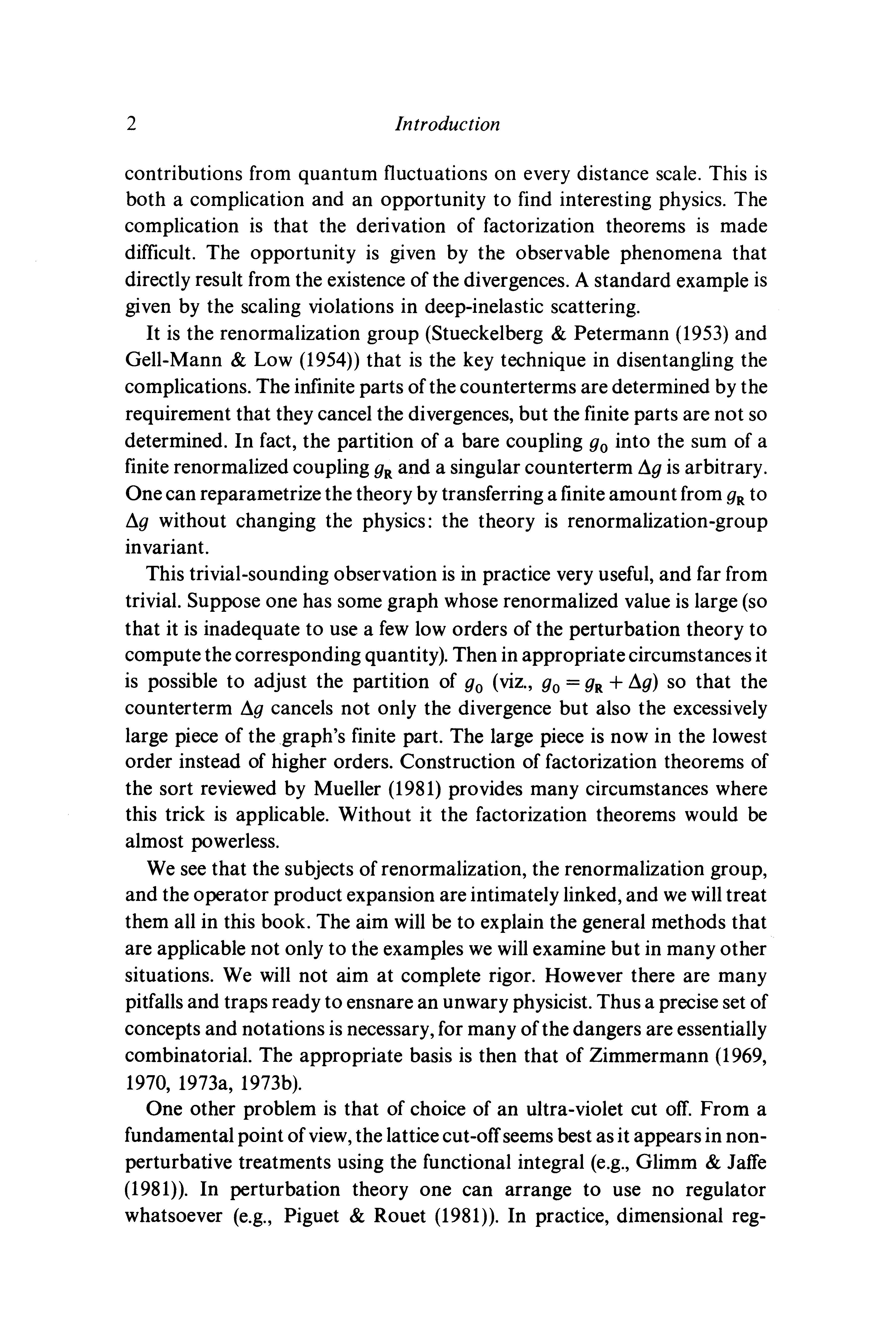
contributions from quantum fluctuations on every distance scale. This is both a complication and an opportunity to find interesting physics. The complication is that the derivation of factorization theorems is made difficult. The opportunity is given by the observable phenomena that directly result from the existence of the divergences. A standard example is given by the scaling violations in deep-inelastic scattering.
It is the renormalization group (Stueckelberg & Petermann (1953) and Gell-Mann & Low (1954)) that is the key technique in disentangling the complications. The infinite parts of the counterterms are determined by the requirement that they cancel the divergences, but the finite parts are not so determined. In fact, the partition of a bare coupling g 0 into the sum of a finite renormalized coupling gRand a singular counterterm llg is arbitrary. One can reparametrize the theory by transferring a finite amount from gR to !lg without changing the physics: the theory is renormalization-group invariant.
This trivial-sounding observation is in practice very useful, and far from trivial. Suppose one has some graph whose renormalized value is large (so that it is inadequate to use a few low orders of the perturbation theory to compute the corresponding quantity). Then in appropriate circumstances it is possible to adjust the partition of g0 (viz., g0 = gR + llg) so that the counterterm !lg cancels not only the divergence but also the excessively large piece of the graph's finite part. The large piece is now in the lowest order instead of higher orders. Construction of factorization theorems of the sort reviewed by Mueller (1981) provides many circumstances where this trick is applicable. Without it the factorization theorems would be almost powerless.
We see that the subjects of renormalization, the renormalization group, and the operator product expansion are intimately linked, and we will treat them all in this book. The aim will be to explain the general methods that are applicable not only to the examples we will examine but in many other situations. We will not aim at complete rigor. However there are many pitfalls and traps ready to ensnare an unwary physicist. Thus a precise set of concepts and notations is necessary, for many of the dangers are essentially combinatorial. The appropriate basis is then that of Zimmermann (1969, 1970, 1973a, 1973b).
One other problem is that of choice of an ultra-violet cut off. From a fundamental point of view, the lattice cut-off seems best as it appears in nonperturbative treatments using the functional integral (e.g., Glimm & Jaffe (1981)). In perturbation theory one can arrange to use no regulator whatsoever (e.g., Piguet & Rouet (1981)). In practice, dimensional reg-
Introduction 3
ularization has deservedly become very popular. This consists of replacing the physical space-time dimensionality 4 by an arbitrary complex number d. The main attraction of this method is that virtually no violence is done to the structure of a Feynman graph; a second attraction is that it also regulates infra-red divergences. The disadvantage is that the method has not been formulated outside of perturbation theory (at least not yet). Much of the treatment in this book, especially the examples, will be based on the use of dimensional regularization. However it cannot be emphasized too strongly that none of the fundamental results depend on this choice.
2
Quantum field theory
Most of the work in this book will be strictly perturbative. However it is important not to consider perturbation theory as the be-ali and end-all of field theory. Rather, it must be looked on only as a systematic method of approximating a complete quantum field theory, with the errors under control. So in this chapter we will review the foundations of quantum field theory starting from the functional integral.
The purpose of this review is partly to set out the results on which the rest of the book is based. It will also introduce our notation. We will also list a number of standard field theories which will be used throughout the book. Some examples are physical theories of the real world; others are simpler theories whose only purpose will be to illustrate methods in the absence of complications.
The use of functional integration is not absolutely essential. Its use is to provide a systematic basis for the rest of our work: the functional integral gives an explicit solution of any given field theory. Our task will be to investigate a certain class of properties of the solution.
For more details the reader should consult a standard textbook on field theory. Of these, probably the most complete and up-to-date is by ltzykson & Zuber (1980); this includes a treatment of the functional integral method. Other useful references include: Bjorken & Drell (1966), Bogoliubov & Shirkov (1980), Lurie (1968), and Ramond (1981).
2.1 Scalar field theory
The simplest quantuP1 field theory is that of a single real scalar field cf>(x 11). The theory is defined by canonically quantizing a classical field theory. This classical theory is specified by a Lagrangian density:
from which follows the equation of motion
Here P(c/J) is a function of c/J(x), which we generally take to be a polynomial like P(c/J) = m 2 c/J 2 /2 +gc/J 4 /4!, and P'(c/J) =dP/dc/J. (Note that we use units with h = c = 1.)
In the Hamiltonian formulation ofthe same theory, we define a canonical momentum field: n(x) =oft' ocjJjot,
and the Hamiltonian
Physically, we require that a theory have a lowest energy state. If it does not then all states are unstable against decay into a lower energy state plus a collection of particles. If the function P(c/J) has no minimum, then the formula (2.1.4) implies that just such a catastrophic situation exists (Baym (1960)). Thus we require the function P(c/J) to be bounded below.
Quantization proceeds in the Heisenberg picture by reinterpreting c/J(x) as a hermitian operator on a Hilbert space satisfying the canonical equaltime commutation relations, i.e.,
[n(x), c/J(y)] = - i<5( 31(i- ji), } .f o o 1 X =y [c/J(x),c/J(y)] = [n(x),n(y)] =0 · (2.1.5)
The Hamiltonian is still given by (2.1.4) so the equation of motion (2.1.2) follows from the Heisenberg equation of motion ioc/Jfot = [ c/J, HJ. (2.1.6)
A solution to the theory is specified by stating what the space of states is and by giving the manner in which cjJ acts on the states. We will construct a solution by use of the functional integral. It should be noted that c/J(x) is in general not a well-behaved operator, but rather it is an operator-valued distribution. Physically that means that one cannot measure c/J(x) at a single point, but only averages of c/J(x) over a space-time region. That is, (2.1.7)
for any complex-valued function f(x), is an operator. Now, products of distributions do not always make sense (e.g., <5(x) 2 ). In particular, the Hamiltonian H involves products of fields at the same point. Some care is needed to define these products properly; this is, in fact, the subject of renormalization, to be treated shortly.
The following properties of the theory are standard:
Quantum field theory
(1) The theory has a Poincare-invariant ground state IO), called the vacuum.
(2) The states and the action of 4> on them can be reconstructed from the time-ordered Green's functions
(2.1.8)
The T-ordering symbol means that the fields are written in order of increasing time from right to left.
(3) The Green's functions have appropriate causality properties, etc., so that they are the Green's functions of a physically sensible theory. Mathematically, these properties are summarized by the Wightman axioms (Streater & Wightman (1978)).
Bose symmetry of the ¢-field means that the Green's functions are symmetric under interchange of any of the x's. From the equations of motion of 4> and from the commutation relations can be derived equations of motion for the Green's functions. The simplest example is D,G 2 (y,x) + (OI TP'(¢(y))¢(x)IO> = - ic5( 4>(x- y). (2.1.9)
For a general (N +I)-point Green's function, we haveN c5-functions on the right: OyGN+ 1 (y, Xp .•. , xN) + (OI T P'(¢(y))¢(x 1 ) ••• ¢(xN)IO> N =- ii c5( 4 >(y- xi)GN_ 1 (x 1 , ••• ,xi_ 1 ,xi+ 1>· • ,xN). j=l (2.1.10)
This equation summarizes both the equations of motion and the commutation relations. Solving the theory for the Green's functions means in essence solving this set of coupled equations. It is in fact the Green's functions that are the easiest objects to compute. All other properties of the theory can be calculated once the Green's functions are known.
2.2 Functional-integral solution
The solution of a quantum field theory is a non-trivial problem in consistency. Only two cases are elementary: free field theory (P = m2 ¢ 2 /2), and the case of one space-time dimension, d = 1. The case d = 1 is a rather trivial field theory, for it is just the quantum mechanics of a particle with Heisenberg position operator ¢(t) in a potential P(¢). (In Section 2.1, we explained the cased = 4. It is easy to go back and change the formulae to be valid for a general value of d.)
2.2 Functional-integral solution 7
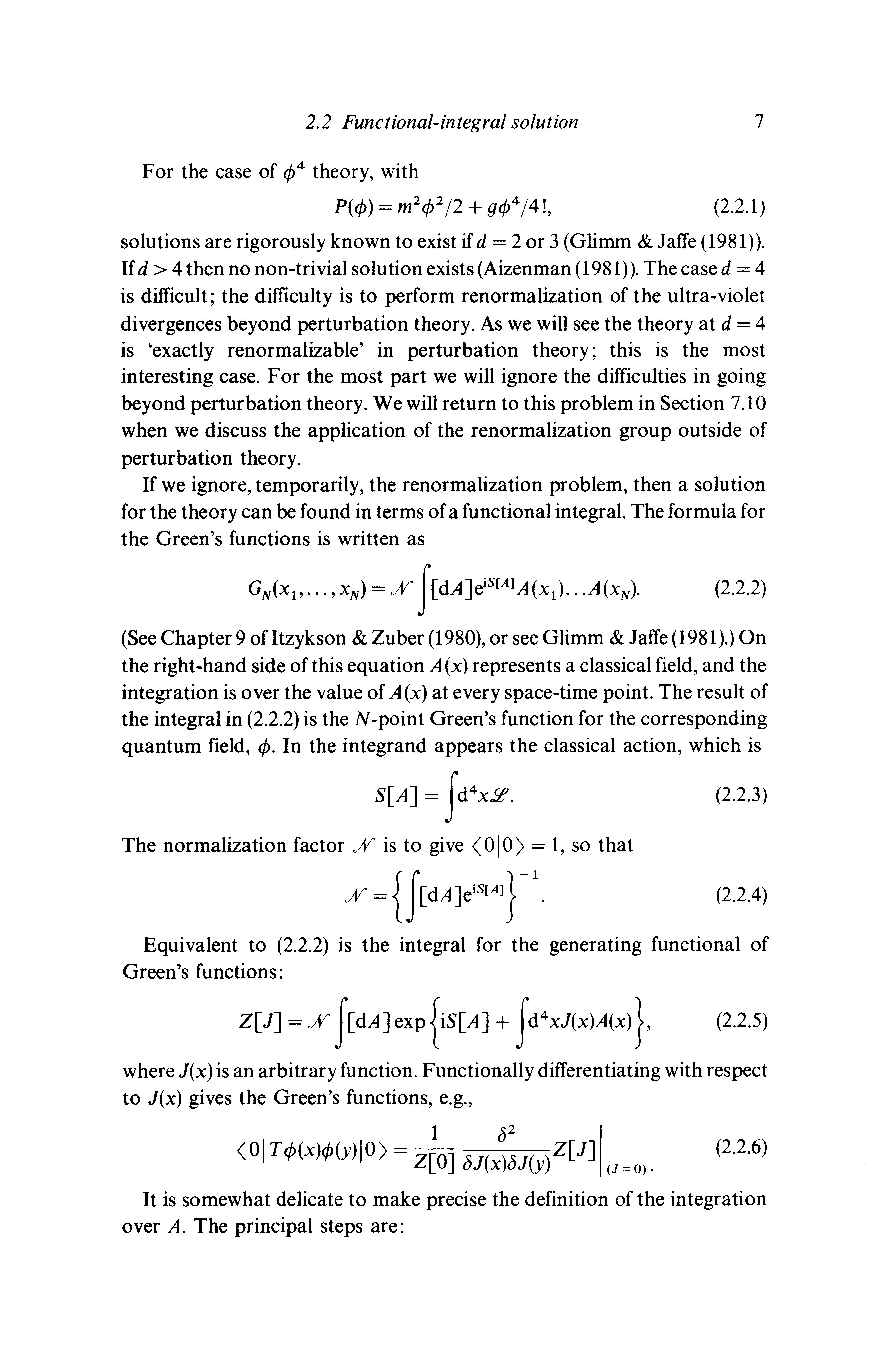
For the case of ¢ 4 theory, with P(¢) = m2 ¢ 2 /2 + g¢ 4 /4 !, (2.2.1) solutions are rigorously known to exist if d = 2 or 3 (Glimm & Jaffe (1981)). If d > 4 then no non-trivial solution exists(Aizenman (1981)). The cased= 4 is difficult; the difficulty is to perform renormalization of the ultra-violet divergences beyond perturbation theory. As we will see the theory at d = 4 is 'exactly renormalizable' in perturbation theory; this is the most interesting case. For the most part we will ignore the difficulties in going beyond perturbation theory. We will return to this problem in Section 7.10 when we discuss the application of the renormalization group outside of perturbation theory.
If we ignore, temporarily, the renormalization problem, then a solution for the theory can be found in terms of a functional integral. The formula for the Green's functions is written as
(See Chapter9 ofltzykson &Zuber (1980), or see Glimm & Jaffe (1981).) On the right-hand side of this equation A (x) represents a classical field, and the integration is over the value of A(x) at every space-time point. The result of the integral in (2.2.2) is theN-point Green's function for the corresponding quantum field, ¢. In the integrand appears the classical action, which is S[A] = Jd 4 x2. (2.2.3)
The normalization factor% is to give (OIO> = 1, so that % = { f(dA JeiS[AJ}- 1 (2.2.4)
Equivalent to (2.2.2) is the integral for the generating functional of Green's functions:
Z[J] =% f[dAJ exp {is[ A] + fd 4 xJ(x)A(x) }· (2.2.5) where J(x) is an arbitrary function. Functionally differentiating with respect to J(x) gives the Green's functions, e.g., 1 ()2 I (OI T¢(x)¢(y)IO> = Z[OJ bJ(x)bJ(y)Z[J] <J=O>· (2.2.6)
It is somewhat delicate to make precise the definition of the integration over A. The principal steps are:
Quantum .field theory
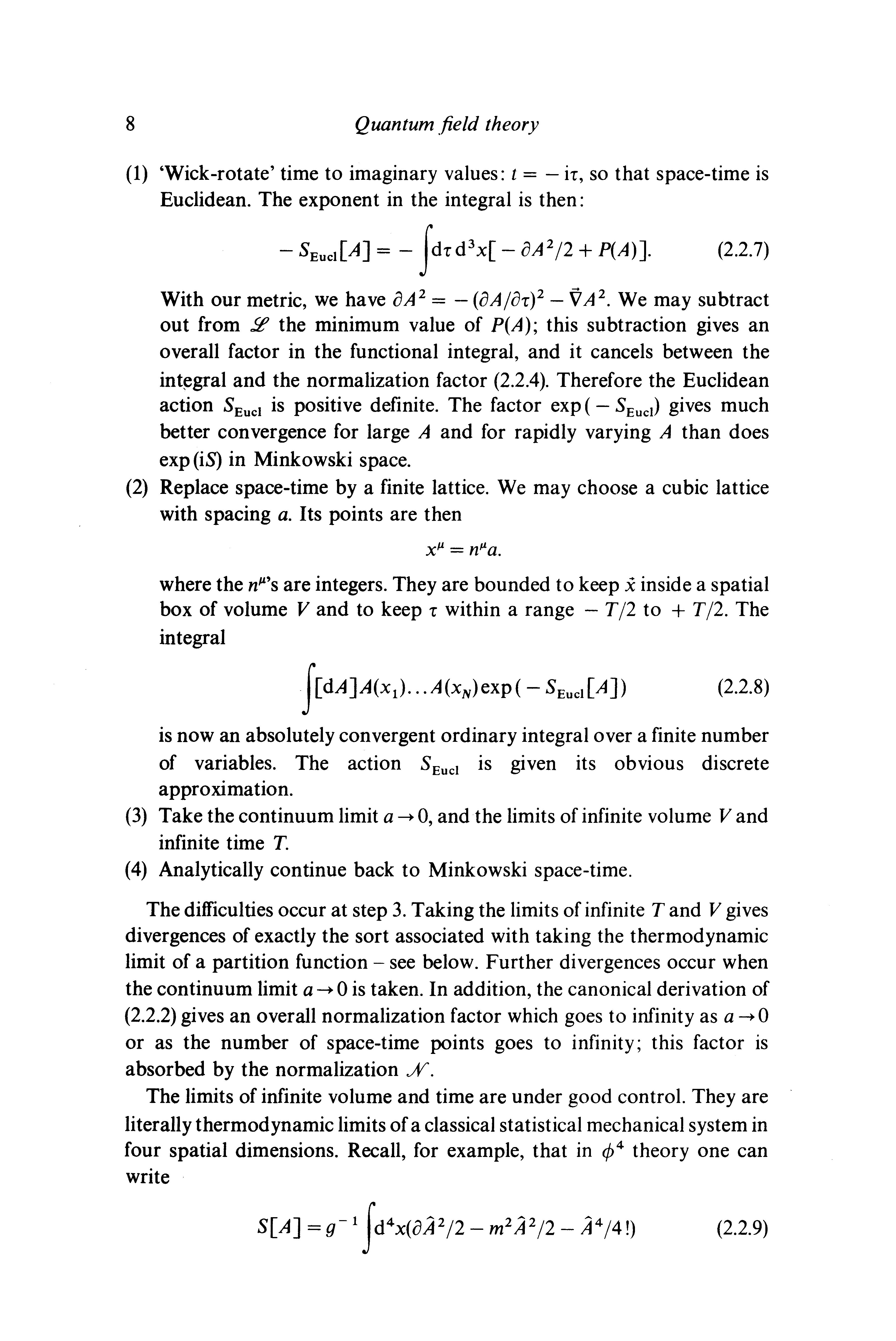
(1) 'Wick-rotate' time to imaginary values: l = - ir, so that space-time is Euclidean. The exponent in the integral is then: - SEucl[AJ =- Jdrd 3 x[- oA 2 /2 + P(A)]. (2.2.7)
With our metric, we have oA 2 = - (oAjor) 2 - VA 2 • We may subtract out from !f? the minimum value of P(A); this subtraction gives an overall factor in the functional integral, and it cancels between the and the normalization factor (2.2.4). Therefore the Euclidean action SEuci is positive definite. The factor exp ( - SEuci) gives much better convergence for large A and for rapidly varying A than does exp (iS) in Minkowski space.
(2) Replace space-time by a finite lattice. We may choose a cubic lattice with spacing a. Its points are then where the are integers. They are bounded to keep x inside a spatial box of volume V and to keep r within a range - T j2 to + T /2. The integral J[dA]A(x 1 ) •.. A(xN)exp(- SEuci[A]) (2.2.8)
is now an absolutely convergent ordinary integral over a finite number of variables. The action SEuci is given its obvious discrete approximation.
(3) Take the continuum limit a--> 0, and the limits of infinite volume V and infinite time T.
(4) Analytically continue back to Minkowski space-time.
The difficulties occur at step 3. Taking the limits of infinite T and V gives divergences of exactly the sort associated with taking the thermodynamic limit of a partition function- see below. Further divergences occur when the continuum limit a--> 0 is taken. In addition, the canonical derivation of (2.2.2) gives an overall normalization factor which goes to infinity as a--> 0 or as the number of space-time points goes to infinity; this factor is absorbed by the normalization%.
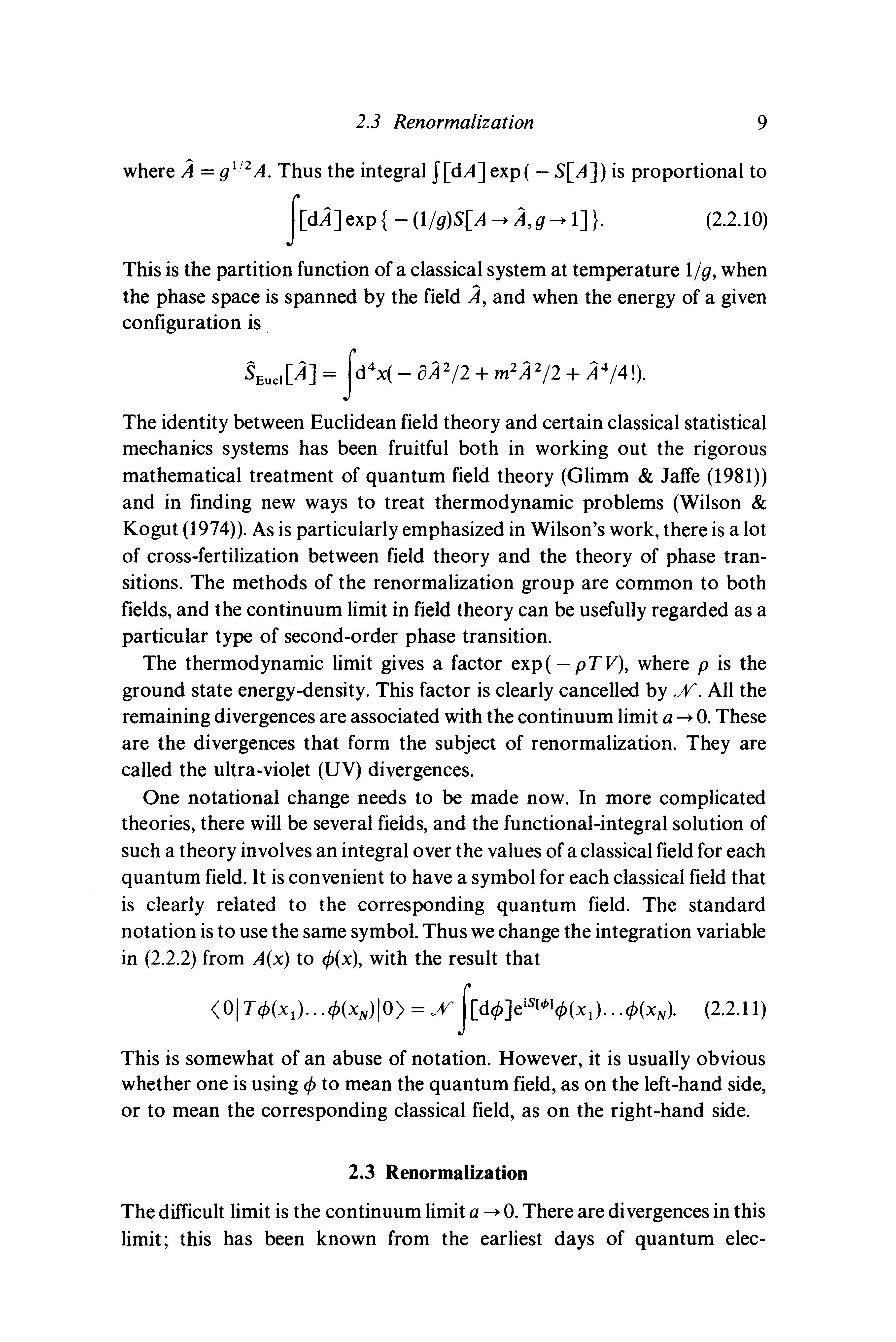
The limits of infinite volume and time are under good control. They are literally thermodynamic limits of a classical statistical mechanical system in four spatial dimensions. Recall, for example, that in ¢ 4 theory one can write (2.2.9)
where A = g 112 A. Thus the integral J[ dA] exp ( - S[ A J) is proportional to J[dA]exp{ -(1/g)S[A --+A,g-->1]}. (2.2.10)
This is the partition function of a classical system at temperature 1/g, when the phase space is spanned by the field A, and when the energy of a given configuration is
SEuci[A]= Jd 4 x(-oA 2 /2+m 2 A2 /2+A 4 /4!).
The identity between Euclidean field theory and certain classical statistical mechanics systems has been fruitful both in working out the rigorous mathematical treatment of quantum field theory (Glimm & Jaffe (1981)) and in finding new ways to treat thermodynamic problems (Wilson & Kogut (1974)). As is particularly emphasized in Wilson's work, there is a lot of cross-fertilization between field theory and the theory of phase transitions. The methods of the renormalization group are common to both fields, and the continuum limit in field theory can be usefully regarded as a particular type of second-order phase transition.
The thermodynamic limit gives a factor exp(- pTV), where p is the ground state energy-density. This factor is clearly cancelled by JV. All the remaining divergences are associated with the continuum limit a--+ 0. These are the divergences that form the subject of renormalization. They are called the ultra-violet (UV) divergences.
One notational change needs to be made now. In more complicated theories, there will be several fields, and the functional-integral solution of such a theory involves an integral over the values of a classical field for each quantum field. It is convenient to have a symbol for each classical field that is clearly related to the corresponding quantum field. The standard notation is to use the same symbol. Thus we change the integration variable in (2.2.2) from A(x) to ¢(x), with the result that
This is somewhat of an abuse of notation. However, it is usually obvious whether one is using¢ to mean the quantum field, as on the left-hand side, or to mean the corresponding classical field, as on the right-hand side.
2.3 Renormalization
The difficult limit is the continuum limit a--+ 0. There are divergences in this limit; this has been known from the earliest days of quantum elec-
Quantum field theory
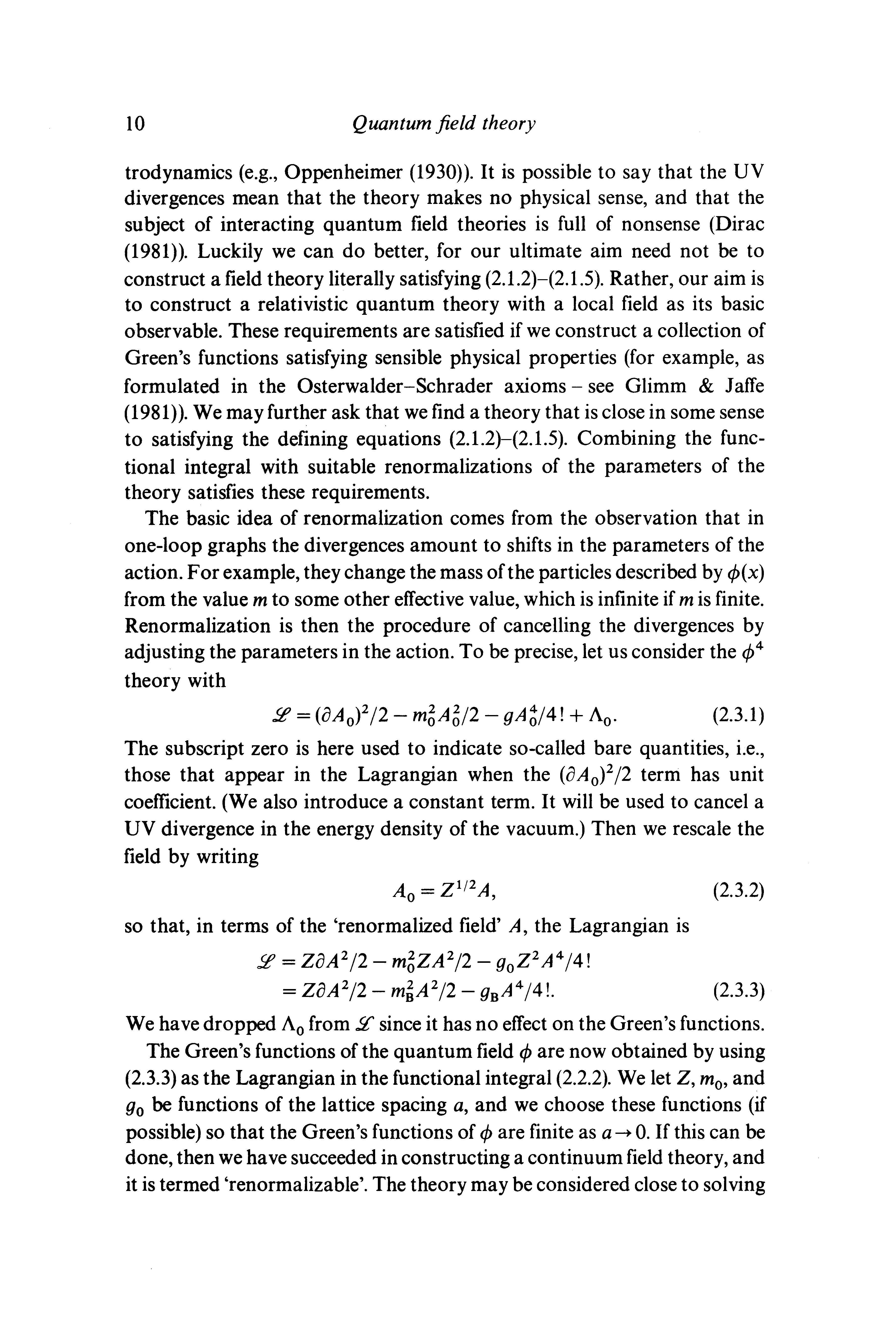
trodynamics (e.g., Oppenheimer (1930)). It is possible to say that the UV divergences mean that the theory makes no physical sense, and that the subject of interacting quantum field theories is full of nonsense (Dirac (1981)). Luckily we can do better, for our ultimate aim need not be to construct a field theory literally satisfying (2.1.2)-(2.1.5). Rather, our aim is to construct a relativistic quantum theory with a local field as its basic observable. These requirements are satisfied if we construct a collection of Green's functions satisfying sensible physical properties (for example, as formulated in the Osterwalder-Schrader axioms- see Glimm & Jaffe (1981)). We may further ask that we find a theory that is close in some sense to satisfying the defining equations (2.1.2)-(2.1.5). Combining the functional integral with suitable renormalizations of the parameters of the theory satisfies these requirements.
The basic idea of renormalization comes from the observation that in one-loop graphs the divergences amount to shifts in the parameters of the action. For example, they change the mass of the particles described by </J(x) from the value m to some other effective value, which is infinite if m is finite. Renormalization is then the procedure of cancelling the divergences by adjusting the parameters in the action. To be precise, let us consider the ¢ 4 theory with (2.3.1)
The subscript zero is here used to indicate so-called bare quantities, i.e., those that appear in the Lagrangian when the (oA 0 ) 2 /2 term has unit coefficient. (We also introduce a constant term. It will be used to cancel a UV divergence in the energy density of the vacuum.) Then we rescale the field by writing
A 0 = Z 1 i 2 A, (2.3.2)
so that, in terms of the 'renormalized field' A, the Lagrangian is 2' = ZoA 2 /2- g0 Z 2 A 4 /4! = ZoA 2 /2- g8 A4 /4!. (2.3.3)
We have dropped A 0 from!£ since it has no effect on the Green's functions.
The Green's functions of the quantum field <jJ are now obtained by using (2.3.3) as the Lagrangian in the functional integral (2.2.2). We let Z, m0 , and g 0 be functions of the lattice spacing a, and we choose these functions (if possible) so that the Green's functions of <jJ are finite as a--+ 0. If this can be done, then we have succeeded in constructing a continuum field theory, and it is termed 'renormalizable'. The theory may be considered close to solving
(2.1.2)-(2.1.5). This is because the theory is obtained by taking a discrete (i.e., lattice) version of the equations and then taking a somewhat odd continuum limit.
We will call m0 the bare mass, and g0 the bare coupling, and we will call Z the wave-function, or field-strength, renormalization. It is also common to call m8 and g8 the bare mass and coupling; but for the sake of consistency we will not do this in this book.
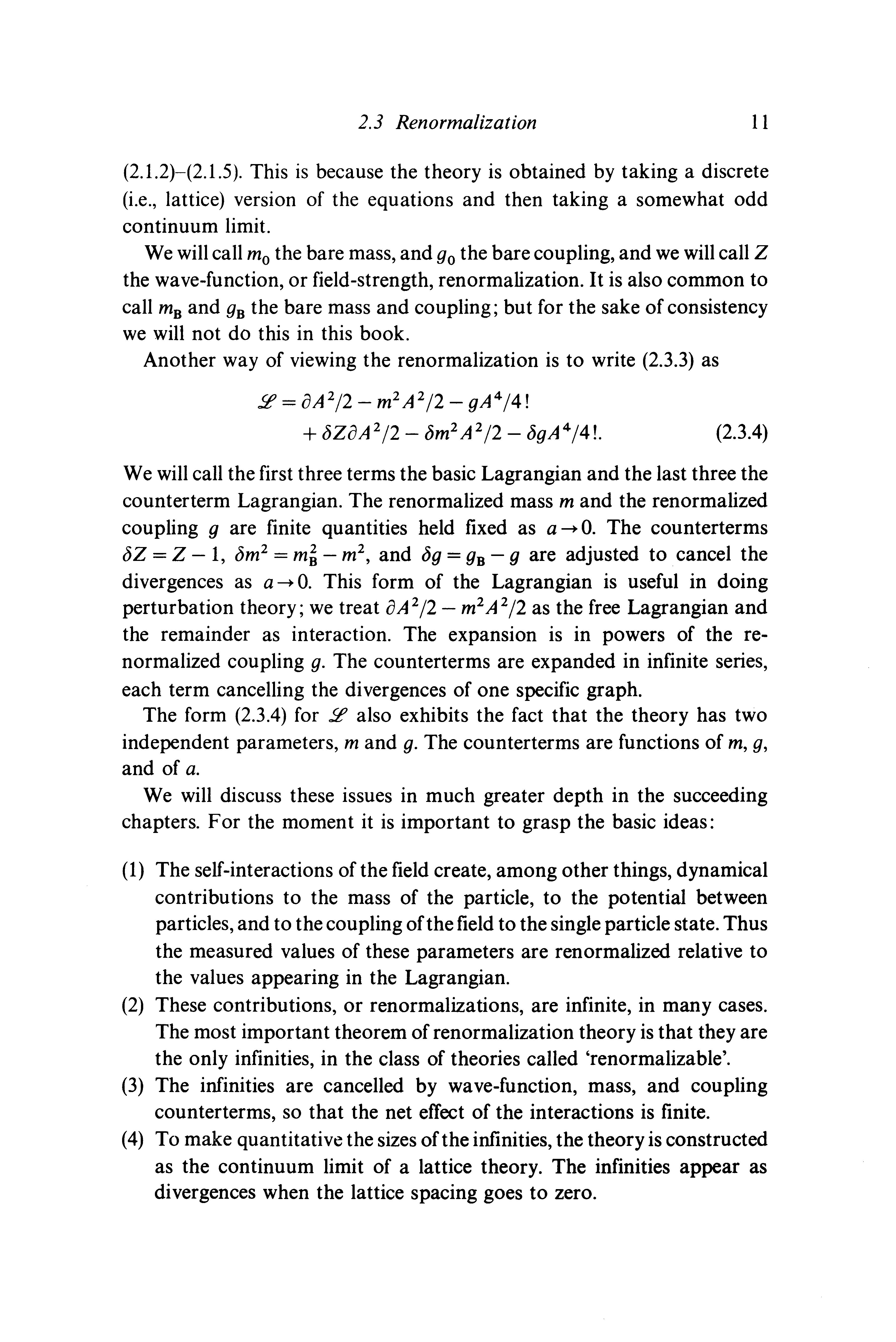
Another way of viewing the renormalization is to write (2.3.3) as
!£ = oA 2 /2- m 2 A 2 /2- gA 4 /4! + bZoA 2 /2- bm 2 A 2 /2- bgA 4 /4!. (2.3.4)
We will call the first three terms the basic Lagrangian and the last three the counterterm Lagrangian. The renormalized mass m and the renormalized coupling g are finite quantities held fixed as a-+ 0. The counterterms [JZ = Z -1, bm 2 = m 2 , and Jg = g8 - g are adjusted to cancel the divergences as a-+ 0. This form of the Lagrangian is useful in doing perturbation theory; we treat oA 2 /2- m 2 A 2 /2 as the free Lagrangian and the remainder as interaction. The expansion is in powers of the renormalized coupling g. The counterterms are expanded in infinite series, each term cancelling the divergences of one specific graph.
The form (2.3.4) for !£ also exhibits the fact that the theory has two independent parameters, m and g. The counterterms are functions of m, g, and of a.
We will discuss these issues in much greater depth in the succeeding chapters. For the moment it is important to grasp the basic ideas:
(1) The self-interactions of the field create, among other things, dynamical contributions to the mass of the particle, to the potential between particles, and to the coupling ofthe field to the single particle state. Thus the measured values of these parameters are renormalized relative to the values appearing in the Lagrangian.
(2) These contributions, or renormalizations, are infinite, in many cases.
The most important theorem of renormalization theory is that they are the only infinities, in the class of theories called 'renormalizable'.
(3) The infinities are cancelled by wave-function, mass, and coupling counterterms, so that the net effect of the interactions is finite.
(4) To make quantitative the sizes of the infinities, the theory is constructed as the continuum limit of a lattice theory. The infinities appear as divergences when the lattice spacing goes to zero.
Quantum .field theory
2.4 Ultra-violet regulators
In the last sections we showed how to construct field theories by defining the functional integral as the continuum limit of a lattice theory. Ultraviolet divergences appear as divergences when the lattice spacing, a, goes to zero, and are removed by renormalization counterterms. The lattice therefore is a regulator, or cut-off, for the UV divergences.
To be able to discuss the divergences quantitively and to construct a theory involving infinite renormalizations, it is necessary to use some kind of UV cut-off. Then the theory is obtained as an appropriate limit when the cut-off is removed. There are many possible ways of introducing a cut-off, of which going to a lattice is only one example. The lattice appears to be very natural when working with the functional integral. But it is cumbersome to use within perturbation theory, especially because of the loss of Poincare in variance. There are two other very standard methods of making an ultraviolet cut-off: the Pauli- Villars method, and dimensional regularization.
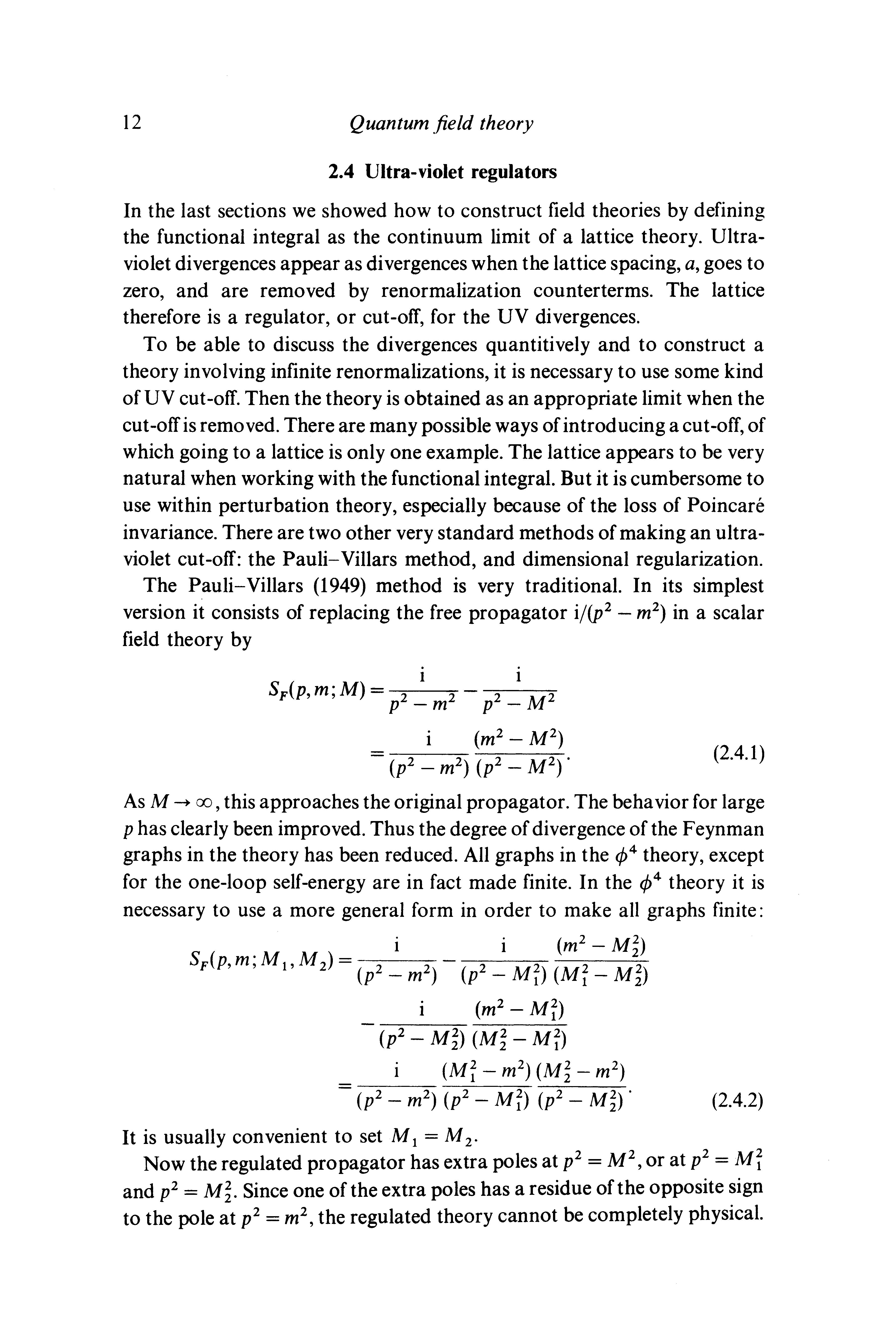
The Pauli- Villars (1949) method is very traditional. In its simplest version it consists of replacing the free propagator ij(p 2 - m2 ) in a scalar field theory by
As M-> oo, this approaches the original propagator. The behavior for large p has clearly been improved. Thus the degree of divergence of the Feynman graphs in the theory has been reduced. All graphs in the ¢ 4 theory, except for the one-loop self-energy are in fact made finite. In the ¢ 4 theory it is necessary to use a more general form in order to make all graphs finite:
S ( m. M M ) - i i (mzF p, ' I' 2 - (p2- m2)- (p2- Mi) (Mi- MD (m2- Mi) (p 2 - Mi) (Mi- m2 ) m 2 ) --;;------;;(p2 _ m2) (p2 _ Mi} (p2 _ · (2.4.2)
It is usually convenient to set M 1 = M 2 •
Now the regulated propagator has extra poles at p2 = M 2 , or at p2 = Mf and p 2 = Since one of the extra poles has a residue ofthe opposite sign to the pole at p 2 = m2 , the regulated theory cannot be completely physical.
Equations of motion for Green's functions
It is normally true that a theory with an ultra-violet cut-off has some unphysical features.
Perhaps the most convenient regulator for practical calculations is dimensional regularization. There it is observed that the UV divergences are removed by going to a low enough space-time dimension d, so d is treated as a continuous variable. In perturbation theory this can be done consistently (Wilson (1973)), as we will see when we give a full treatment of dimensional regularization in Chapter 4. However it has not been possible to make it work non-perturbatively, so it cannot at present be regarded as a fundamental method.
Since it is only the renormalized theory with no cut-off that is of true interest, the precise method of cut-off is irrelevant. In fact, all methods of ultra-violet cut-off are equivalent, at least in perturbation theory. The differences are mainly a matter of practical convenience (or of personal taste). Thus dimensional regularization is very useful for perturbation theory. But the lattice method is maybe most powerful when working beyond perturbation theory; it is possible, for example, to compute the function.al integral numerically by Monte-Carlo methods (Creutz (1980, 1983), and Creutz & Moriarty (1982)).
Within perturbation theory one need not even use a cut-off. Zimmermann (1970, 1973a) has shown how to apply the renormalization procedure to the integrands rather than to the integrals for Feynman graphs. The lack of fundamental dependence on the procedure of cut-off is thereby made manifest. The application of this procedure to gauge theories, especially, is regarded by most people as cumbersome.
2.5 Equations of motion for Green's functions
We have defined a collection of Green's functions by the functional integral (2.2.2). (Implicit in the definition are a certain number of limiting procedures, as listed below (2.2.6).) This definition we will take as the basis for the rest of our work. First we must check that it in fact gives a solution of the theory. This means, in particular, that we are to derive the equations of motion (2.1.10) for the Green's functions, thus ensuring that both the operator equation of motion (2.1.2) and the commutation relations (2.1.5) hold. (For the remainder of this chapter we will not specify the details of how renormalization affects these results.)
It is convenient to work with the generating functional (2.2.5). We make the change of variable A(x)--+ A(x) + ef(x), where e is a small number, and f(x) is an arbitrary function of x". Since the integration measure is invariant
Quantum .field theory
under this shift, the value of the integral is unchanged:
which is equivalent to (2.1.9). Note that in the fourth line we have exchanged the order of integration and of differentiation for the 0 Y term. We have also used the normalization condition (2.2.4). It is important that the derivative of the quantum field (next-to-last line) is outside the time ordering, and c5Sjc5cf>(y) in the last line is defined to be a shorthand for the combination of operators in the previous line.