Employment Relations Theory & Practice 4th Ed. 4th Edition
Mark Bray
https://ebookmass.com/product/employment-relations-theorypractice-4th-ed-4th-edition-mark-bray/
ebookmass.com
Marketing 7th Edition Levy Grewal
https://ebookmass.com/product/marketing-7th-edition-levy-grewal/


ebookmass.com
Defects in Two-Dimensional Materials Rafik Addou
https://ebookmass.com/product/defects-in-two-dimensional-materialsrafik-addou/
ebookmass.com
The Political Economy of Emerging Markets and Alternative Development Paths Judit Ricz
https://ebookmass.com/product/the-political-economy-of-emergingmarkets-and-alternative-development-paths-judit-ricz/
ebookmass.com


e6%96%af%ef%bc%88john/ ebookmass.com
Over and above their precision, there is something more to numbers-maybe a little magic-that makes them fun to study. The fun is in the conceptualization more than the calculations, and we are fortunate that we have the computer to do the drudge work. This allows students to concentrate on the ideas. In other words, the computer allows the instructor to teach the poetry of statistics and not the plumbing.
Computing
To take advantage of the computer, one needs a good statistical package. We use Stata, which is available from the Stata Corporation in College Station, Texas. We find this statistical package to be one of the best on the market today; it is user-friendly, accurate, powerful, reasonably priced, and works on a number of different platforms, including Windows, Unix, and Macintosh. Furthermore, the output from this package is acceptable to the Federal Drug Administration in New Drug Approval submissions. Other packages are available, and this book can be supplemented by any one of them. In this second edition, we also present output from SAS and Mini tab in the Further Applications section of each chapter. We strongly recommend that some statistical package be used.
Some of the review exercises in the text require the use of the computer. To help the reader, we have included the data sets used in these exercises both in Appendix B and on a CD at the back of the book. The CD contains each data set in two different formats: an ASCII file (the "raw" suffix) and a Stata file (the "dta" suffix). There are also many exercises that do not require the computer. As always, active learning yields better results than passive observation. To this end, we cannot stress enough the importance of the review exercises, and urge the reader to attempt as many as time permits.
New to the Second Edition
This second edition includes revised and expanded discussions on many topics throughout the book, and additional figures to help clarify concepts. Previously used data sets, especially official statistics reported by government agencies, have been updated whenever possible. Many new data sets and examples have been included; data sets described in the text are now contained on the CD enclosed with the book. Tables containing exact probabilities for the binomial and Poisson distributions (generated by Stata) have been added to Appendix A. As previously mentioned, we now incorporate computer output from SAS and Minitab as well as Stata in the Further Applications sections. We have also added numerous new exercises, including questions reviewing the basic concepts covered in each chapter.
Acknowledgements
A debt of gratitude is owed a number of people: Harvard University President Derek Bok for providing the support which got this book off the ground, Dr. Michael K. Martin for calculating Tables A.3 through A.8 in Appendix A, and John-Paul Pagano for
3 Numerical Summary Measures 38
3. 7 Measures of Central Tendency 3 8
3.1.1 Mean 38
3.1.2 Median 41
3.1.3 Mode 42
3.2 Measures of Dispersion 44
3.2.1 Range 44
3.2.2 Interquartile Range 44
3.2.3 Variance and Standard Deviation 46
3.2.4 Coefficient of Variation 48
3.3 Grouped Data 48
3.3.1 Grouped Mean 49
3.3.2 Grouped Variance 51
3.4 Chebychev's Inequality 52
3.5 Further Applications 54
3.6 Review Exercises 59
Bibliography 64
4 Rates and Standardization 66
4. 7 Rates 66
4.2 Standardization of Rates 70
4.2.1 Direct Method of Standardization 72
4.2.2 Indirect Method of Standardization 74
4.2.3 Use of Standardized Rates 75
4.3 Further Applications 84
4.3.1 Direct Method of Standardization 86
4.3.2 Indirect Method of Standardization 86
4.4 Review Exercises 89
Bibliography 95
5 Life Tables 97
5. 7 Computation of the Life Table 97
5.1.1 Column 1 97
5.1.2 Column 2 99
77.3 Further Applications 272
77.4 Review Exercises 278 Bibliography 282
J2
Analysis of Variance 285
72. 7 One-Way Analysis of Variance 285
12.1.1 The Problem 285 12.1.2 Sources ofVariation 288
72.2 Multiple Comparisons Procedures 292
72.3 Further Applications 294
72.4 Review Exercises 298 Bibliography 30 1
13
Nonparametric Methods
73. 7 The Sign Test 302
73.2 The Wilcoxon Signed-Rank Test
73. 3 The Wilcoxon Rank Sum Test 302 305 308
73.4 Advantages and Disadvantages of Non parametric Methods 3 122
73.5 Further Applications 3 12
73.6 Review Exercises 3 17 Bibliography 32 1
J4
Inference on Proportions 323
74. 7 Normal Approximation to the Binomial Distribution 324
74.2 Sampling Distribution of a Proportion 325
74. 3 Confidence Intervals 327
74.4 Hypothesis Testing 329
74.5 Sample Size Estimation 330
74.6 Comparison of Two Proportions 332
74.7 Further Applications 335
74.8 Review Exercises 338 Bibliography 34 1
21 Survival Analysis 488
2 7. 7 The Life Table Method 489
27.2 The Product-Limit Method 495
21.3 The Log-Rank Test 499
27.4 Further Applications 503
21.5 Review Exercises 5 11
Bibliography 5 1 2
22 Sampling Theory 5 1 4
22.7 Sampling Schemes 5 1 4
22.1.1 Simple Random Sampling 515
22.1.2 Systematic Sampling 515
22.1.3 Stratified Sampling 516
22.1.4 Cluster Sampling 517
22.1.5 Nonprobability Sampling 517
22.2 Sources of Bias 5 1 7
22.3 Further Applications 520
22.4 Review Exercises 524
Bibliography 525
Appendix A
Tables A-1
Appendix B
Data Sets B-1
Index 1-1
Data that take on only two distinct values require special attention. In the health sciences, one of the most common examples of this type of data is the categorization of being either alive or dead. If we denote the former state by 0 and the latter by 1, we are able to classify a group of individuals using these numbers and then to average the results. In this way, we can summarize the mortality associated with the group. Chapter 4 deals exclusively with measurements that assume only two values. The notion of dividing a group into smaller subgroups or classes based on a characteristic such as age or gender is introduced as well. We might wish to study the mortality of females separately from that of males, for example. Finally, this chapter investigates techniques that allow us to make valid comparisons among groups that may differ substantially in composition.
Chapter 5 introduces the life table, one of the most important techniques available for study in the health sciences. Life tables are used by public health professionals to characterize the well-being of a population, and by insurance companies to predict how long a particular individual will live. In this chapter, the study of mortality begun in Chapter 4 is extended to incorporate the actual time to death for each individual; this results in a more refined analysis. Knowing these times to death also provides a basis for calculating the survival curve for a population. This measure of longevity is used frequently in clinical trials designed to study the effects of various drugs and surgical treatments on survival time.
In summary, the first five chapters of the text demonstrate that the extraction of important information from a collection of numbers is not precluded by the variability among them. Despite this variability, the data often exhibit a certain regularity as well. For example, if we look at the annual mortality rates of teenagers in the United States for each of the last ten years, we do not see much variation in the numbers. Is this just a coincidence, or is it indicative of a natural underlying stability in the mortality rate? To answer questions such as this, we need to study the principles of probability.
Probability theory resides within what is known as an axiomatic system: we start with some basic truths and then build up a logical system around them. In its purest form, the system has no practical value. Its practicality comes from knowing how to use the theory to yield useful approximations. An analogy can be drawn with geometry, a subject that most students are exposed to relatively early in their schooling. Although it is impossible for an ideal straight line to exist other than in our imaginations, that has not stopped us from constructing some wonderful buildings based on geometric calculations. The same is true of probability theory: although it is not practical in its pure form, its basic principles-which we investigate in Chapter 6---can be applied to provide a means of quantifying uncertainty.
One important application of probability theory arises in diagnostic testing. Uncertainty is present because, despite their manufacturers' claims, no available tests are perfect. Consequently, there are a number of important questions that must be answered. For instance, can we conclude that every blood sample that tests positive for HIV actually harbors the virus? Furthermore, all the units in the Red Cross blood supply have tested negative for HIV; does this mean that there are no contaminated samples? If there are contaminated samples, how many might there be? To address questions such as these, we must rely on the average or long-term behavior of the diagnostic tests; probability theory allows us to quantify this behavior.
Chapter 7 extends the notion of probability and introduces some common probability distributions. These mathematical models are useful as a basis for the methods studied in the remainder of the text.
The early chapters of this book focus on the variability that exists in a collection of numbers. Subsequent chapters move on to another form of variability-the variability that arises when we draw a sample of observations from a much larger population. Suppose that we would like to know whether a new drug is effective in treating high blood pressure. Since the population of all people in the world who have high blood pressure is very large, it is extremely implausible that we would have either the time or the resources necessary to examine every person. In other situations, the population may include future patients; we might want to know how individuals who will ultimately develop a certain disease as well as those who currently have it will react to a new treatment. To answer these types of questions, it is common to select a sample from the population of interest and, on the basis of this sample, infer what would happen to the group as a whole.
If we choose two different samples, it is unlikely that we will end up with precisely the same sets of numbers. Similarly, if we study a group of children with congenital heart disease in Boston, we will get different results than if we study a group of children in Rome. Despite this difference, we would like to be able to use one or both of the samples to draw some conclusion about the entire population of children with congenital heart disease. The remainder of the text is concerned with the topic of statistical inference.
Chapter 8 investigates the properties of the sample mean or average when repeated samples are drawn from a population, thus introducing an important concept known as the central limit theorem. This theorem provides a foundation for quantifying the uncertainty associated with the inferences being made.
For a study to be of any practical value, we must be able to extrapolate its findings to a larger group or population. To this end, confidence intervals and hypothesis testing are introduced in Chapters 9 and 10. These techniques are essentially methods for drawing a conclusion about the population we have sampled, while at the same time having some knowledge of the likelihood that the conclusion is incorrect. These ideas are first applied to the mean of a single population. For instance, we might wish to estimate the mean concentration of a certain pollutant in a reservoir supplying water to the surrounding area, and then determine whether the true mean level is higher than the maximum concentration allowed by the Environmental Protection Agency. In Chapter 11, the theory is extended to the comparison of two population means; it is further generalized to the comparison of three or more means in Chapter 12. Chapter 13 continues the development of hypothesis testing concepts, but introduces techniques that allow the relaxation of some of the assumptions necessary to carry out the tests. Chapters 14, 15, and 16 develop inferential methods that can be applied to enumerated data or countssuch as the numbers of cases of sudden infant death syndrome among children put to sleep in various positions-rather than continuous measurements.
Inference can also be used to explore the relationships among a number of different attributes. If a full-term baby whose gestational age is 39 weeks is born weighing 4 kilograms, or 8.8 pounds, no one will be surprised. If the baby's gestational age is only 22
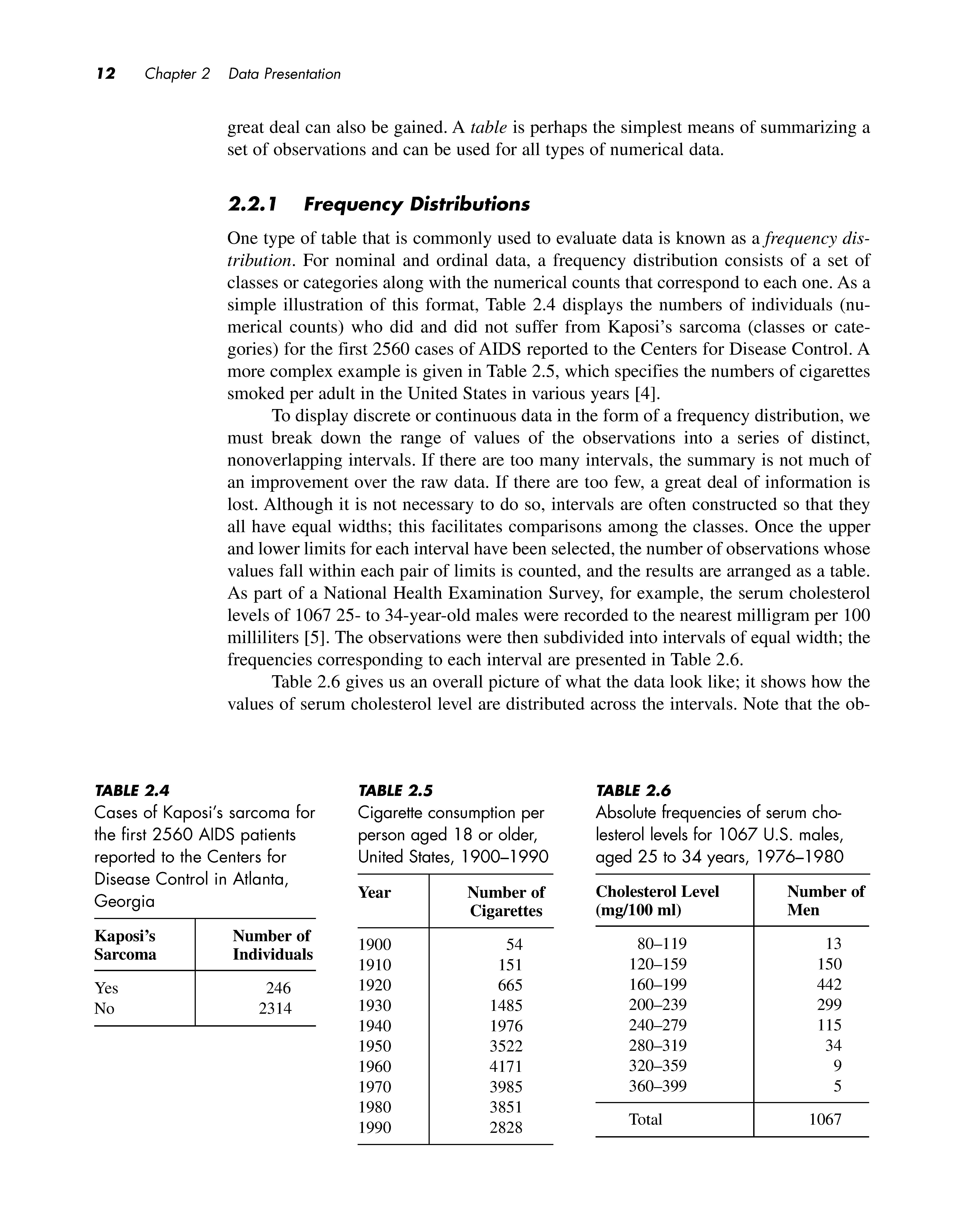
Every study or experiment yields a set of data. Its size can range from a few measurements to many thousands of observations . A complete set of data , however, will not necessarily provide an investigator with information that can easily be interpreted. For example , Table 2.1 lists by row the first 2560 cases of acquired immunodeficiency syndrome (AIDS) reported to the Centers for Disease Control and Prevention [1] . Each individual was classified as either suffering from Kaposi ' s sarcoma , designated by a 1, or not suffering from the disease, represented by a 0 . (Kaposi ' s sarcoma is a tumor that affects the skin , mucous membranes , and lymph nodes.) Although Table 2.1 displays the entire set of outcomes , it is extremely difficult to characterize the data . We cannot even identify the relative proportions of Os and 1s . Between the raw data and the reported results of the study lies some intelligent and imaginative manipulation of the numbers , carried out using the methods of descriptive statistics
Descriptive statistics are a means of organizing and summarizing observations. They provide us with an overview of the general features of a set of data. Descriptive statistics can assume a number of different forms ; among these are tables, graphs , and numerical summary measures . In this chapter, we discuss the various methods of displaying a set of data. Before we decide which technique is the most appropriate in a given situation , however, we must first determine what kind of data we have .