Overviewofmeshlessmethods
Chapteroutline
1.1Whyweneedmeshlessmethods 3
1.2Reviewofmeshlessmethods 6
1.3Basicideasofthemethodof fundamentalsolutions 8
1.3.1Weightedresidualmethod 8
1.3.2Methodoffundamental solutions 10
1.4ApplicationtothetwodimensionalLaplaceproblem 13
1.4.1Problemdescription 13
1.4.2MFSformulation 14
1.4.3Programstructureand sourcecode 18
1.4.3.1Inputdata 19
1.4.3.2Computationof coefficientmatrix 19
1.4.3.3Solvingthe resultingsystemof linearequations 19
1.4.3.4Sourcecode 20
1.4.4Numericalexperiments 24
1.4.4.1Circulardisk 24
1.4.4.2Interiorregion surroundedbya complexcurve 29
1.4.4.3Biased hollowcircle 33
1.5Somelimitationsfor implementingthemethodof fundamentalsolutions 34
1.5.1Dependenceof fundamentalsolutions 37
1.5.2Locationofsourcepoints 37
1.5.3Ill-conditioningtreatments 39
1.5.3.1Tikhonovregularizationmethod 39
1.5.3.2Singularvalue decomposition 39
1.5.4Inhomogeneousproblems 41
1.5.5Multipledomainproblems 41 1.6Extendedmethodoffundamental solutions 43 1.7Outlineofthebook
1.1Whyweneedmeshlessmethods
Initialand/orboundary valueproblemssuchasheattransfer,wavepropagation,elasticity,fluidflow,piezoelectricity,andelectromagneticscanbefound inalmosteveryfieldofscienceandengineeringapplicationsandaregenerally modeledbypartialdifferentialequations(PDEs)withprescribedboundary conditionsand/orinitialconditionsinagivendomain.ThusPDEsare fundamentaltothemodelingofphysicalproblems.Consequently,clear understandingofthephysicalmeaningofsolutionsoftheseequationshas becomeveryimportanttoengineersandmathematicians,sothatthesolutions
canbeusedtoexplainnaturalphenomenaortodesignanddevelopnew structuresandmaterials.
Tothisend,theoreticalandexperimentalmethodswerefirstdeveloped. However,PDEsusuallyinvolvehigher-orderpartialdifferentialstospatialor timevariables,buttheoreticalanalysisisoperableonlyforproblemswithsimple expressionsofPDEs,simpledomainshapes,andsimpleboundaryconditions. Mostengineeringproblemscannotbesolvedanalytically.Besides,dueto limitationstoexperimentalconditions,mostengineeringproblemscannotbe testedexperimentally,andeveniftheproblemcanbetested,theprocessistimeconsumingandexpensive;moreover,notalloftherelevantinformationcanbe measuredexperimentally.Hence,waystofindgoodapproximatesolutionsusing numericalmethodsshouldbeveryinterestingandhelpful.
Currently,solutionsofordinary/boundaryvalueproblemscanbecomputed directlyoriterativelyusingnumericalmethods,suchasthefiniteelement method(FEM) [1 3],thehybridfiniteelementmethod(HFEM) [4 8],the boundaryelementmethod(BEM) [9 12],thefinitedifference/volumemethod (FDM/FVM) [2,13],andthemeshlessmethod [14,15],etc.
Amongthesemethods,conventionalelement-dependentmethodssuchas theFEM,theHFEM,theBEM,andtheFVMrequiredomainorboundary elementpartitiontomodelcomplexmultiphysicsproblems.Forexample,in theclassicFEM,whichwasoriginallydevelopedbyRichardCourantin1943 forstructuraltorsionanalysis [16],acontinuumwithacomplexboundary shapecangeometricallybedividedintoafinitenumberofelements,generally termedfiniteelements.Theseindividualfiniteelementsareconnectedthrough nodestoformatopologicalmesh.Ineachindividualelement,theproper interpolatingfunctionischosentoapproximatetherealdistributionofthe physicalfield.Thenallelementsareintegratedintoaweak-formintegral functionaltoproducethesolvingsystemofequations,sothatthenodalfieldas theprimaryvariableinthefinalsolvingsystemcanbefullydetermined.Dueto suchfeaturesasversatilityofmeshingforcomplexgeometryandflexibilityof solvingstrategyforcomplexproblems,theFEMhasbecomeoneofthemost robustandwell-developedproceduresforboundary/ordinaryvalueproblems, andithasbeensuccessfullyappliedinmanyengineeringapplications [1]
Thereare,however,someinherentlimitationsforuseoftheFEM.Firstly, meshgenerationisusuallytime-consumingintheFEM,andonemustspend muchtimeandeffortforcomplexdatamanagementandtreatment.Secondly, meshgenerationinvolvescomplexalgorithms,andthisisnotalwayspossible forproblemswithcomplexdomains,especiallythree-dimensionalgeometricallycomplexdomains.Insomecases,usersmustmakepartitionstocreate relativelyregularsubdomainsforapplyingmeshgeneration.Thirdly,asa displacement-basednumericalmethod,theFEMcanrelativelyaccurately predictdisplacement,ratherthanstressthatinvolveshigher-orderderivatives ofdisplacementtospatialvariables.Moreover,stressesobtainedintheFEM areoftendiscontinuousacrossthecommoninterfaceofadjacentelements,
becauseoftheelement-wisecontinuousnatureofthedisplacementfield assumedintheFEMformulation.Specialsmoothedtreatmenttechniquesare requiredinthepostprocessingstagetorecoverstresses.Fourthly,numerical accuracyintheFEMissignificantlydependentonmeshdensity,soa remeshingoperationisusuallyrequiredtoachieveadesiredaccuracy.Multiplemeshingtrialsmaybeneededforthatpurpose.Moreimportantly,for largedeformationproblems,adaptivemeshisrequiredtoavoidelement distortionduringdeformation.Theremeshingprocessateachstepoftenleads toadditionalcomputationaltimeaswellasdegradationofaccuracyinthe solution.Finally,itisdifficultfortheFEMtoeffectivelysimulatecrack growthandmaterialfracturebecausethecontinuouselementsintheFEM cannoteasilymodeldiscontinuousfields.AlltheselimitationscanbeattributedtotheuseofelementsormeshintheFEMformulation.
AsanalternativetotheFEM,theelement-dependentBEMattemptstofind numericalsolutionsofboundaryintegralequationsbyincorporatingelement discretizationoverthedomainboundary [2,10,17,18].IntheBEM,the boundaryintegralequationmayberegardedasanexactsolutionofthegoverningpartialdifferentialequationoftheproblem,towhichthefundamental solutionshouldbeexplicitlyavailable,anditcanbederivedbyintroducing thephysicaldefinitionoffundamentalsolutiontoincludeboundaryvaluesin therepresentationformula.SuchdistinguishingfeaturesgivetheBEMthe followingadvantagesovertheFEM:(1)Onlytheboundaryofthedomain needstobediscretized;asaresult,verysimpledatainputandstorageare involved.(2)Thesolutionintheinteriorofthedomainisapproximatedwitha ratherhighconvergencerateandaccuracy.(3)Exteriorproblemswith unboundeddomainsaremoreproperlysolvedbytheBEM,becausetheremote conditioncanbeexactlysatisfied.However,theBEMalsoexperiencessome difficulties.Forexample,theBEMisgreatlydependentofthefundamental solutionofthepartialdifferentialequation.So,problemswithinhomogeneities ornonlineardifferentialequationsareingeneralnoteasilyhandledbypure BEM.Additionally,theBEMrequiresmoremathematicalfoundation, comparedtotheFEM,toobtaintheboundaryintegralequationandevaluate boundaryintegrals,becausethekernelsinboundaryintegralsareingeneral singular.AllthesedisadvantageslimitBEMapplications,sosometimes couplingofothermethodsmustbeimplemented [19]
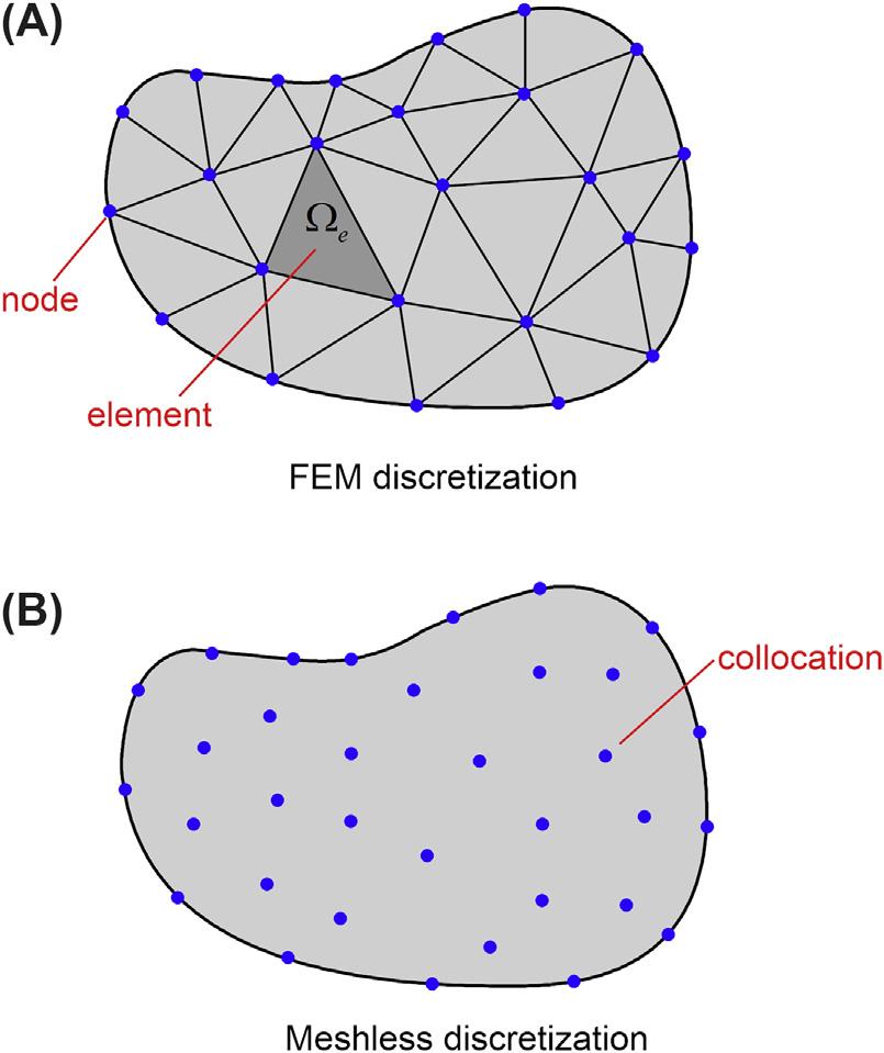
Incontrast,meshlessmethodsbasedonboundaryand/orinteriorcollocationsinadomaincanremovelimitationssuchasintheFEMandBEM, significantlyreducingtheeffortofmodeldiscretizationpreparation.To illustratethis, Fig.1.1 displaysdomaindiscretizationbyelementsandcollocationsintheconventionalFEMandthemeshlessmethod.Ingeneral,theterm “meshlessmethod”referstotheclassofnumericaltechniquesthatdonot requireanypredefinedmeshinformationfordomaindiscretization,relying simplyoneitherglobalorlocalizedinterpolationonnonorderedspatial pointsscatteredwithintheproblemdomainaswellasonitsboundaries.
Thesescatteredpointsarenotgeometricallyconnectedtoformamesh.Thus meshlessmethodspresentgreatpotentialforengineeringapplications.
1.2Reviewofmeshlessmethods
MeshlessmethodsareusedtosolvePDEinstrongorweakformbyarbitrarily distributedcollocationsinthesolutiondomain,andthesepointscontributeto theapproximationbyassumedglobalorlocalbasisfunctions.
AsintheclassificationofFEMandBEM,meshlessmethodsmayalsobe dividedintotwocategories:domain-typemeshlessmethodsandboundary-type meshlessmethods.Domain-typemeshlessmethods,asthenameimplies, employarbitrarilydistributedinteriorandboundarycollocationstorepresentthe problemdomainanditsboundary.Thenthefieldvariable(e.g.,displacement, temperature,pressure)atanyfieldpointwithintheproblemdomainisinterpolatedusingfunctionvaluesatalocalorglobalsetofnodesaroundthefield point.Subsequently,aweak-formintegralequationsuchastheGalerkinintegral equationorastrong-formcollocationequationisintroducedtoincludethe assumedfieldvariablesinproducingasystemofequationsassociatedwiththe variables.Strong-formdomain-typemeshlessmethods,includesmoothed particlehydrodynamics(SPH) [20],thefinitepointmethod(FPM) [21], thepointcollocationmethod(PCM) [22],theKansacollocationmethod [23], andtheleast-squarescollocationmeshlessmethod [24],etc.Weak-formdomaintypemeshlessmethodsincludethediffuseelementmethod(DEM) [25],
FIGURE1.1 FEMandmeshlessdiscretizationina2Ddomain.
theelement-freeGalerkinmethod(EFGM) [26],thereproducingkernelparticle method(RKPM) [27],partitionofunityfiniteelementmethods(PUFEM) [28], theHp-meshlesscloudsmethod [29],themeshlesslocalPetrov-Galerkinmethod (MLPG) [30],andthepointinterpolationmethod(PIM) [31],etc.Incontrastto thestrong-frommeshlessmethods,themeshlessmethodsbasedontheweak formaremorerobustandsteady.However,thelattergenerallyinvolvemore complexformulations.
Unlikedomain-typemeshlessmethods,boundary-typemeshlessmethods requireonlyboundarycollocationinthecomputation.Inthatcase,the T-completefunctionbasis [5,6] orthefundamentalsolutionbasis [10] is typicallyemployedtoapproximatethefieldvariable,soitcanexactlysatisfy thegoverningequationsoftheproblem.Forexample,Zhangetal.presented thesolutionprocedureofthehybridboundarynodemethod(BNM) [32] that combinesthemodifiedvariationalfunctionalandthemovingleast-square (MLS)approximationbasedonlyonagroupofarbitrarilydistributed boundarynodes.Thismethodisaweak-formmethodandonlyinvolves integrationcomputationovertheboundary.However,MLSinterpolationslack thedeltafunctionproperty,soitisdifficulttosatisfytheboundaryconditions accuratelyintheBNM.InanimprovementovertheBNM,theboundarypoint interpolationmethod(BPIM) [33] employsshapefunctionshavingthe Kroneckerdeltafunctionproperty,soboundaryconditionscanbeenforcedas easilyasintheconventionalBEM.
Besides,somepureboundarycollocationmethodsexist,includingthe methodoffundamentalsolutions(MFS) [14,34],boundaryparticlemethod (BPM) [35,36],andTrefftzboundarycollocationmethod(TBCM) [37,38]. Amongthese,theMFSisthemostpowerfulandpopular,whenfundamental solutionsofaproblemareexplicitlydefined.Itwasinitiallyintroducedby KupradzeandAleksidzein1964 [39].Overthepast30years,MFShasbeen widelyusedforthenumericalapproximationofalargevarietyofphysical problems [34].ThegeneralconceptoftheMFSisthatthesolution(field variable)approximatedbyalinearcombinationoffundamentalsolutionswith respecttosourcepointslocatedoutsidethesolutiondomaincanexactlysatisfy thegoverningpartialdifferentialequationoftheproblem,soonlyboundary conditionsatboundarycollocationsneedtobesatisfied.TheMFSinheritsall theadvantagesoftheBEM [10];forexample,itdoesnotrequirediscretization overthedomain,unlikedomainmeshdiscretizationmethodssuchasthe FEM.Moreover,unliketheBEM,integrationsoverthedomainboundaryare avoided.Thesolutionintheinteriorofthedomainisevaluatedalsowithout anyadditionalintegrationequation.Furthermore,thederivativesofthesolutionarecalculateddirectlyfromtheMFSrepresentation.Moreimportantly, implementationoftheMFSisveryeasyanddirect,evenforproblemsin three-dimensionalandirregulardomains,andonlyalittledatapreparationis required.Besides,highnumericalaccuracyandfastconvergencehasbeen proven [40 42].Thus,itisemployedanddiscussedinthisbook.
1.3Basicideasofthemethodoffundamentalsolutions
ToillustratethebasicconceptoftheMFS,thefollowingtwo-dimensional homogeneouspartialdifferentialequationisconsidered:
where L isapartialdifferentialoperator, x ¼ (x, y)isanarbitrarypointina boundeddomain U 3 ℝ2 , ℝ2 denotestheEuclidean2-space,and u isthe unknownfieldvariable.Itisnotedthatinthebookwesometimeswrite x ¼ (x1, x2)ratherthan x ¼ (x, y)forthesakeofconvenience.
Foracompleteboundaryvalueproblem,theproperboundaryconditions shouldbecomplemented,forexample,
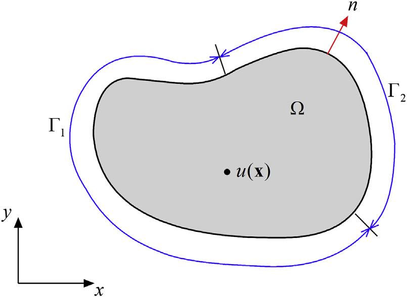
where G1 W G2 ¼ vU, G1 X G2 ¼ B, u and q aregivenfunctions,and n isthe unitnormaltotheboundary vU,asindicatedin Fig.1.2.
1.3.1Weightedresidualmethod
Theboundaryvalueproblem(BVP)describedinthegoverning Eq.(1.1) and theboundaryconditions (1.2) canbesolvedinanapproximatemanner,by whichthefieldvariable u isapproximatedinageneralformby
where fi(x)isthe ithbasisfunctionterm, ai istheunknowncoefficientforthe ithbasisfunctionterm,and m isthenumberofbasisfunctions.
FIGURE1.2 Schematicofboundaryvalueproblem.
Inpractice,theapproximationfunctiongivenin Eq.(1.3) cannotexactly satisfythegoverningequationandtheboundaryconditions,duetothetruncatedapproximation.Hence,substituting Eq.(1.3) into Eqs.(1.1)and(1.2),we usuallyhave
and
Ifthefollowingresidualfunctionscanbedefined,
then Eqs.(1.4)and(1.5) canberespectivelyrewrittenas
and
Theoretically,theproperapproximatefunctionshouldmaketheresiduals ateachpoint x insidethedomainorontheboundaryassmallaspossible. However,suchstrong-formsatisfactionisdifficulttoderive.Inthepractical operation,weusuallyforcetheresidualstozeroinanaveragedsenseby settingtheso-calledweightedintegralsoftheresidualstozero,i.e.,
where wi, vi,and si areasetofgivenweightfunctionscorrespondingtothe ith point,and i ¼ 1,2, ., n.
Intheweightedresidualmethod,theselectionofweightfunctionsdeterminesthetypeandperformanceofnumericalapproximations.Inthisbook, thecollocation-typemeshlessmethodisdiscussed.Inthecollocationmethod, asetofpointsthataredistributedinthedomainarechosenforapproximation, andwecantrytosatisfytheBVPatonlythesepoints,ratherthansatisfying
theBVPinanintegralform.Toobtainthecollocationsolution,weselectthe standardDiracdeltafunctionastheweightfunctionsin Eq.(1.10),i.e.,
where d(x, xi)istheDiracdeltafunctioncenteredatthepoint xi andhasthe followingproperties:
and
Thus,thecollocationmethodcanbederivedfromtheweightedresidual formulationbysubstituting Eq.(1.11) intoit:
whichresultsin
Eq.(1.15) showsthattheresidualsarezeroat n pointschoseninthe problemdomain.Specially,iftheapproximationcanexactlysatisfythegoverning Eq.(1.1),i.e.,theTrefftzapproximationandfundamentalsolution approximationtakenintoaccountinthisbook,thedomainresidual Rg should bezero.Inthatcase, Eq.(1.15) canbereducedto
whichmeansthatonlyboundarycollocationscanbechosentoforcethe boundaryresidualstozeroatthosecollocations.Thiscanberegardedasthe theoreticalbasisoftheMFSdescribednext.
1.3.2Methodoffundamentalsolutions
IntheapplicationoftheMFS,thesolutionofproblemsgovernedby Eqs.(1.1) and(1.2) isapproximatedasalinearcombinationoffundamentalsolutions:
ðxÞz X N j¼1 aj G ðx; xsj Þ¼ Ga; x ˛ U; xsj ;U (1.17) where N isthenumberofsourcepoints fxsj gN j¼1 locatedoutsidethedomain, G*(x, xsj)centeredat xsj isthefundamentalsolutionofthepartialdifferential Eq.(1.1) inthespatialcoordinate x ¼ (x, y) [43,44], aj isthecoefficientfor G*(x, xsj)thatisyettobedetermined,and G ¼½ G ðx; xs1 Þ G ðx; xsN Þ (1.18)
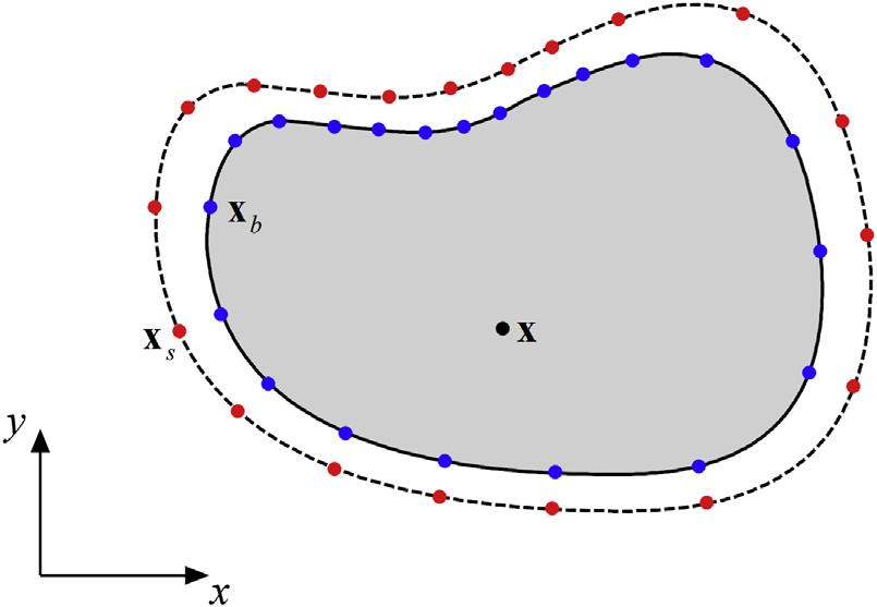
Obviously,theapproximation (1.17) exactlysatisfiesthepartialdifferential Eq.(1.1) duetothenonoverlappingofthesourcepoints xsj ( j ¼ 1,2, , N ) andthefieldpoint x.Therefore,theapproximation (1.17) justneedstosatisfy thespecifiedboundaryconditions (1.2).Todetermineallknowncoefficients in Eq.(1.17),wecollocatetheapproximatesolution (1.17) onafinitesetof boundarypoints{xb1, xb2, ., xbM}˛G,asshownin Fig.1.3. M isthetotal numberofboundarycollocations.If M1 and M2 representthenumberofcollocationsontheboundaries G1 and G2,respectively,and M ¼ M1 þ M2,wehave
where xbi and xbk arecollocationsontheboundarysegment G1 and G2, respectively.
Eq.(1.20) canberewritteninthefollowingmatrixform:
FIGURE1.3 CollocationsintheMFS.
Explicitly,thisleadstoan M N-dimensionalcollocationlinearsystemof equationsthatcangenerallybewrittenas
orinmatrixform
where H isthe M N-dimensionalcollocationmatrixwithelements Hij, a is the N 1vectorofunknowns,and b isthe M 1knownvector.
Toobtainauniquesolutionforthelinearsystemof Eq.(1.25),weusually require M N.If M ¼ N,thelinearsystemof Eq.(1.25) canbesolveddirectly usingtheGaussianeliminationtechniqueoraregularizationtechniquesuchas theTichonovregularizationorthetruncatedsingularvaluedecompositionif thematrix H isill-conditioned,whereasifM > Nwemustemploythelinear least-squaretechniquetoreplacetherectangular M N overdeterminedsystemof Eq.(1.25) withasquare N N determinedsystem.Forexample, minimizationoftheEuclideanerrornormof Eq.(1.25)
fromwhichweobtain
Eq.(1.28) canberewritteninmatrixformas
wherethesuperscript“T”denotesthetransposeofamatrix.
Solving Eq.(1.29) fortheunknowncoefficientvector a,weobtain
andthenthefieldvariableatarbitrarypoint x˛U canbeevaluatedby Eq.(1.17)
Oneoftheobviousadvantagesofsuchamethodisthefactthatthereisno needforanymeshgenerationatanyfunctionevaluation,andonlyboundary collocationsarerequired.Thismeansthatthecomputationiseconomicalin termsoftime.OtheradvantagesoftheMFSincludeitssimpleformulationand highprecisionthatcanbeillustratedbyitsapplicationtotwo-dimensional Laplaceproblems.
1.4Applicationtothetwo-dimensionalLaplaceproblem
ToillustratetheMFSsolutionprocedure,weconsideraLaplaceproblemgiven inatwo-dimensionalCartesiancoordinatedomain.Therelatedsourcecodeis providedtobetterunderstandtheMFSimplementation.
1.4.1Problemdescription
Weconsideraboundedsimplyormultiplyconnectedregion U intheplane xy Forthetwo-dimensionalLaplaceproblemdefinedinthedomain U,the governingpartialdifferentialequationrelatedtothepotentialfunction u canbe writtenas
where
representsthetwo-dimensionalLaplaceoperator,and x ¼ (x, y)isthearbitrary pointintheplane.
Moreover,thegoverning Eq.(1.31) shouldbecomplementedbythe followingboundaryconditionstoformawell-definedBVP: u ¼ f on G
q ¼
on G
where q ¼ vu/vn denotestheoutwardnormalderivativeof u ontheboundary vU,and f and g aregivenvaluesdefinedon G1 and G2,respectively.Here, vU ¼ G1 W G2 and G1 X G2 ¼ B.
TheMFSemploysthefundamentalsolutionofaproblemtoapproximate theunknownpotentialfield u.Therefore,thefundamentalsolutionofthe problemshouldbeexplicitlyformulated.Here,thefundamentalsolutiontothe two-dimensionalLaplaceoperatorin Eq.(1.31) canbegivenby
istheEuclideandistance, xs isasourcepointatwhichaunitsourceintensityis applied,and x isanarbitraryfieldpointinaninfinitetwo-dimensionaldomain.
Correspondingly,thefirst-orderderivativesof u*canbeobtainedas
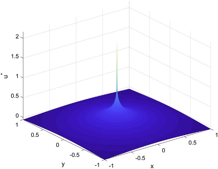
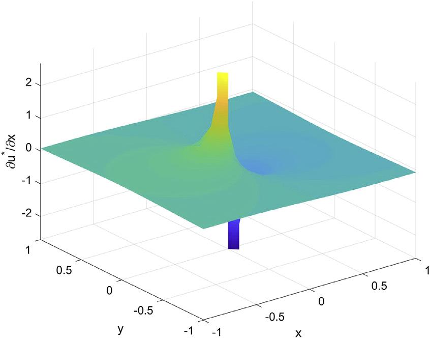
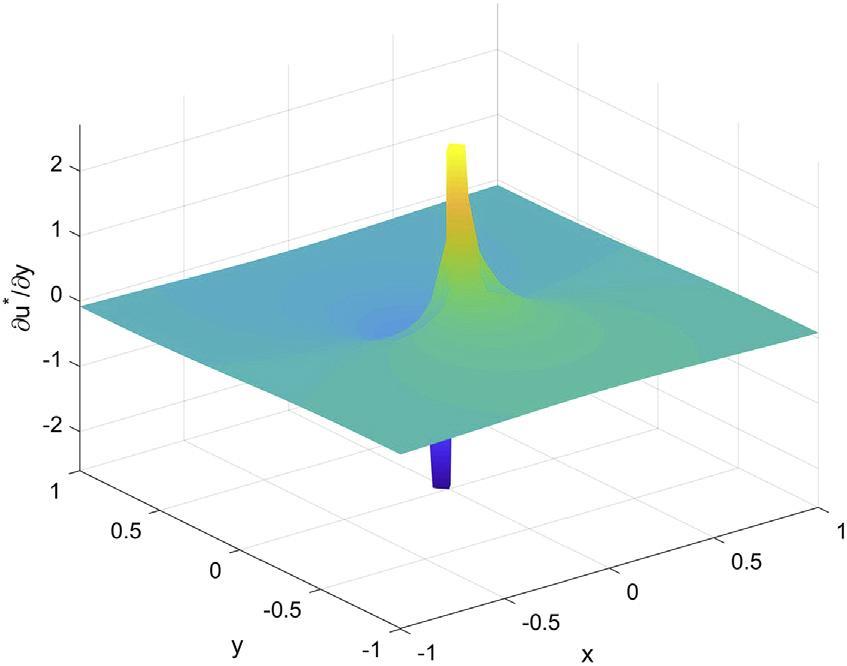
Figs.1.4 1.6 plotthevariationsof u*anditsderivativesforthesource point xs ¼ (0,0),respectively,fromwhichitisobservedthatthefundamental solution u*anditsderivatives vu*/vx and vu*/vy showsingularityatthesource point.Fortunately,thesourcepointcannotoverlapwiththefieldpointinthe theoryofMFS,becauseitisarrangedoutsidethedomainofinterest.
1.4.2MFSformulation
Basedonthefundamentalsolutionoftheproblemgivenin Eq.(1.34),the followingschemefortheimplementationoftheMFScanbeobtained. Choosingthesetofsourcepoints fxsk gN k ¼1 outsidethecomputingdomain U,
FIGURE1.4
FIGURE1.5 Variationof vu*/vx forthetwo-dimensionalLaplaceoperatorat xs ¼ (0,0).
FIGURE1.6 Variationof vu*/vy forthetwo-dimensionalLaplaceoperatorat xs ¼ (0,0).
wecanconstructtheapproximationforthesolution u of Eqs.(1.31)and(1.33) asfollows: uðxÞ¼ X N k ¼1 ak u ðx; xsk Þ (1.37) orinmatrixform: u ¼ Ua (1.38) with
aT ¼½ a1 a2 . aN 1 N (1.40)
Further,thefirst-orderderivativesof u canbeapproximatedas qx ¼ vu vx ¼ X N k ¼1 ak vu ðx; xsk Þ vx ¼ vU vx a qy ¼ vu vy ¼ X N k ¼1
(1.41)
Then,theoutwardnormalderivativeof u on G2 canbeexpressedas
q ¼ vu vn ¼ qx nx þ qy ny ¼ X N k ¼1 ak vu ðx; xsk Þ vx nx þ vu ðx; xsk Þ vy ny
¼ X N k ¼1 ak q ðx; xsk Þ¼ Qa (1.42)
where nx and ny arecomponentsoftheoutwardnormalvector n,and q ðx; xsk Þ ¼ vu ðx; xsk Þ vx nx þ vu ðx; xsk Þ vy ny (1.43) Q ¼½ q ðx; xs1 Þ q ðx; xs2 Þ q ðx; xsN Þ 1 N (1.44)
Intheprecedingapproximations,thecoefficients fak gN k ¼1 canbedeterminedbythesatisfactionoftheseboundaryconditionsatcollocationpointson theboundary vU;thatis,ifwetake N collocations fxk gN k ¼1 on vU andthen imposethegivenboundaryconditions,wehave
uðxk Þ¼ X N k ¼1 ak u ðxk ; xsk Þ¼ f ðxk Þ; xk ˛ G1 ; k ¼ 1; 2; .; N1
qðxk Þ¼ X N k ¼1 ak q ðxk ; xsk Þ¼ gðxk Þ; xk ˛ G2 ; k ¼ 1; 2; .; N2 (1.45)
where N1 and N2 arethenumberofcollocationson G1 and G2,respectively, and N ] N1 þ N2 Eq.(1.45) canberewritteninmatrixnotationas (1.46)
or
(1.47) fromwhichtheapproximatingcoefficientscanbesolvedandthenthequantitiesatanypointinthedomaincanbeevaluatedby Eqs.(1.37)and(1.41) for furtherplottingoranalysis.
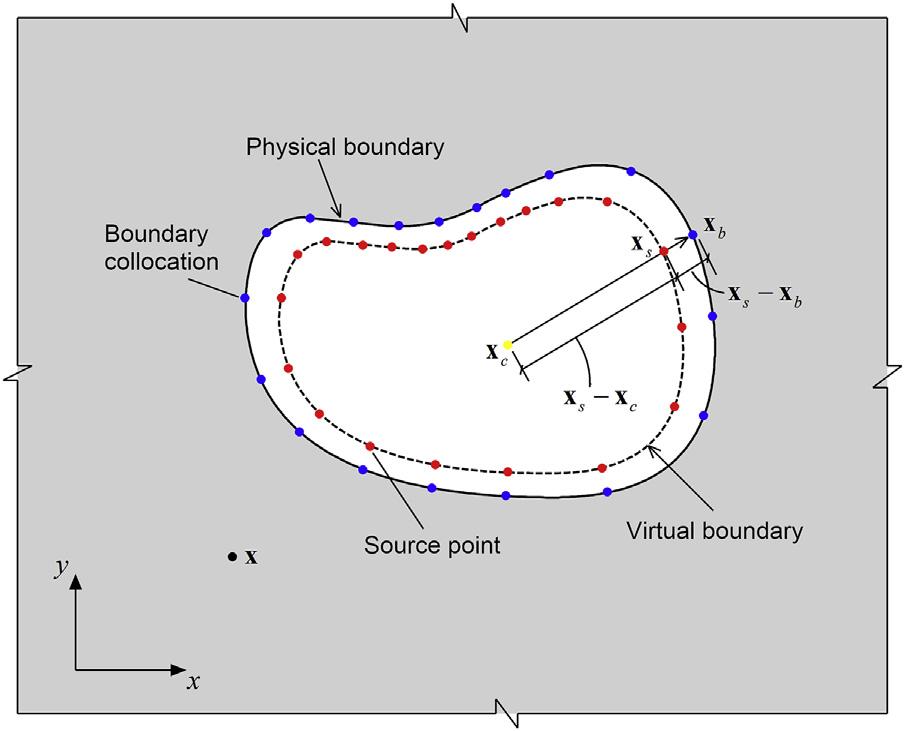
Theuniqueexistenceofapproximatesolutionsfor Eqs.(1.31)and(1.33) of theform (1.37) hasbeenestablishedtheoretically.However,thelocationsof sourcepoints fxsk gN k ¼1 outsidethecomputingdomaincannotbeexplicitly determined.Inpracticalcomputation,wecanusuallyemploythefollowing relationtogeneratethesourcepoint:
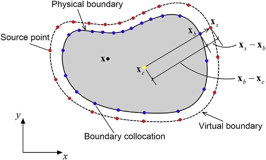
where xs, xb,and xc representthepositionsofsourcepoint,boundarypoint, andcenterpoint,respectively. g denotesthenondimensionalparameterusedto controlthedistancebetweenthesourcepointandtherealboundary.
Obviously, Eq.(1.48) canbeequallyrewrittenas
or
where l ¼ 1 þ g > 0isusuallycalledthesimilarityratiobetweenthevirtual boundarysourcepointslocatedandtherealphysicalboundary.
Eq.(1.50) meansthatthecoordinatesofthesourcepointgeneratedbythe relation (1.48) arescaledmagnificationorshrinkageofthecoordinatesofthe boundarycollocationpoint.Theoretically,forthecaseoftheinteriordomain (see Fig.1.7),thescalingfactor g > 0,whereasforthecaseoftheexterior domain(see Fig.1.8),theparameter g canbechosenintherange( 1,0).For boththeinteriorandexternaldomainproblems,itisfoundthatthecloserthe parameter g isto0,thecloserthevirtualboundaryconnectingthesource pointsistothephysicalboundary.However,fromthecomputationalpointof view,thenumericalaccuracymaydecreaseasthedistancebetweenthevirtual
FIGURE1.8 Illustrationofthelocationsofsourcepointsforexternaldomainproblems.
andphysicalboundariesbecomestoosmall,inwhichcasetheparameter g is closetozero,andtheproblembecomessingularduetothesingularityofthe fundamentalsolutions.Incontrast,asthedistanceofsourcepointsfromthe physicalboundaryincreases,theconditioningnumberofthecollocation matrixofthelinearsolvingsystemofequationsincreases,andtheround-off errorsinfloating-pointarithmeticmaybecomeaconcern.Typically,ifthe parameter g becomesverylarge,theentriesinthecollocationmatrixwillbe closetozero.Therefore,toachieveagoodbalancefortheconditioning numberandthenumericalerrorsgeneratedbytheMFSinpracticalcomputation,theparameter g isgenerallyselectedtobeintherangeof1.0 10.0for interiordomainproblemsand 0.3w 0.8forexternaldomainproblems [34,42,45,46].Inpractice,weusuallyemploy g ¼ 3fortheinteriorcaseand g ¼ 0.5fortheexteriorcase.
1.4.3Programstructureandsourcecode
BasedontheMFSformulationdescribedbefore,MATLABcodecanbe programmedforthenumericalanalysisoftwo-dimensionalLaplaceproblems. Themainsolutionproceduresoftheprogramincludethefollowing:
l Readinputdataandallocateproperarraysizes.
l For eachboundarycollocation do:
l Computecoefficients;
l Assembletoformcoefficientmatrix.
l Solvetheresultingmatrixequationfortheapproximatingcoefficients.
l Computeresultsattestpoints.
l Outputthepotentialanditsderivativesolutions.