Introduction to Mathematical Methods of Analytical Mechanics
Henri Gouin
First published 2020 in Great Britain and the United States by ISTE Press Ltd and Elsevier Ltd
Apart from any fair dealing for the purposes of research or private study, or criticism or review, as permitted under the Copyright, Designs and Patents Act 1988, this publication may only be reproduced, stored or transmitted, in any form or by any means, with the prior permission in writing of the publishers, or in the case of reprographic reproduction in accordance with the terms and licenses issued by the CLA. Enquiries concerning reproduction outside these terms should be sent to the publishers at the undermentioned address:
ISTE Press Ltd
27-37 St George’s Road
Elsevier Ltd
The Boulevard, Langford Lane London SW19 4EU Kidlington, Oxford, OX5 1GB UK UK
www.iste.co.uk
www.elsevier.com
Notices
Knowledge and best practice in this field are constantly changing. As new research and experience broaden our understanding, changes in research methods, professional practices, or medical treatment may become necessary.
Practitioners and researchers must always rely on their own experience and knowledge in evaluating and using any information, methods, compounds, or experiments described herein. In using such information or methods they should be mindful of their own safety and the safety of others, including parties for whom they have a professional responsibility.
To the fullest extent of the law, neither the Publisher nor the authors, contributors, or editors, assume any liability for any injury and/or damage to persons or property as a matter of products liability, negligence or otherwise, or from any use or operation of any methods, products, instructions, or ideas contained in the material herein.
For information on all our publications visit our website at http://store.elsevier.com/
© ISTE Press Ltd 2020
The rights of Henri Gouin to be identified as the author of this work have been asserted by him in accordance with the Copyright, Designs and Patents Act 1988.
British Library Cataloguing-in-Publication Data
A CIP record for this book is available from the British Library Library of Congress Cataloging in Publication Data
A catalog record for this book is available from the Library of Congress ISBN 978-1-78548-315-8
Printed and bound in the UK and US
Preface
Theobjectiveofthisbookistoofferanoverviewofgeometricmethodsofcalculus ofvariationsandhowthiscanbeappliedinanalyticalmechanics.Itisfollowedbythe studyofpropertiesofspacesinmechanicalsystemswithafinitenumberofdegrees offreedom.Thebookwasinspired,inpart,bymethodsproposedbyPierreCasal,a formerProfessorattheFacultyofSciencesofMarseillesUniversity.Thesemethods wereconsideredagainanddevelopedduringacoursethatItaughttostudentsinthe thirdyearoftheAppliedMathematicsBachelor’sprogram.
Themathematicaltoolsusedthroughoutthebookarethoseusedinelementary algebra,analysisanddifferentialgeometry.Thebookdoesnotrequiremathematical toolsthatwouldbebeyondthescopeofathird-yearuniversitystudent(readersmay refer,amongothers,totheworksof(Queysane1971,CoutyandEzra1980,Martin 1967,Brousse1968).
Part1
Inthefirstpartofthebook,wepresentgeometricmethodsusedinthecalculusof variations.Freeextremaorextremathatarerelatedtointegralornon-integral constraintsarestudied.Thesemakeitpossibletointroducetheconceptofthe Lagrange multiplier.Aninitialstudyofthe Hamiltonequations1 associatedwith theconceptofageneratingfunctionfollowsfromthesemethods.Researchintothe geodesicsofsurfacesisalsoanaturalapplicationthatusesdifferentialgeometry. Thesemethodsofdifferentialgeometrycanbeextendedtothecalculationofthe variationofcurvilinearintegrals.Twoformsofvariationscanbemadeandexplicitly discussed:thefirstformusestheconceptofvariationofavectorialderivative;the secondformissimilartofindingtheopticalpathfollowedbylightinamediumwith
1Itshouldbenotedthattheseequationsarelikelytohavebeenwrittenby Huygens,andthe symbol H correspondstohisinitials.
avariablerefractiveindex.Thisleadstothestudyof Descartes’laws and isoperimetricproblems. Noether’stheorem,groupsofinvarianceassociatedwith differentialequationsandtheconceptofa Liegroup arenaturalextensionsofthese calculations.Thus, Fermat’sprinciple,associatedwiththeopticalpathfollowedby light,leadstofindingfirstintegrals.Thetoolsusedarerelatedtotensorcalculations thatbringinthestructureofavectorspaceanditsdualspace.
Part2
Thesecondpartofthebookpresentstheapplicationofthetoolsdiscussedearlier tothemechanicsofmaterialsystemswithafinitenumberofdegreesoffreedom. Afterbrieflyreviewingthe d’Alembertprinciple,weintroducetheconceptof Lagrangiandefinedinspace-timebythehomogeneousLagrangian.Wefindthatthe firstintegralinmechanicsisassociatedwithNoether’stheorem.Thereintroduction ofpartialresultsleadstothe Maupertuisprinciple andtotheintroductionof Riemanniangeometry inthecaseoftheconservationofenergy;thisisthefoundation for deBrogliewavemechanics.Theintegrationmethodsforequationsinmechanics areanalyzedusingthe Jacobimethod anditsapplicationintheimportantcaseof Liouville’sintegrability.Thissectioncontinueswiththeconceptsof angular variables and actionvariables forperiodicandmulti-periodicmotions,presentedby Delaunay,whichareespeciallyusefulincelestialmechanics.Thesecondpart concludeswiththestudyofspaceinanalyticalmechanics,includingvariousphase spaces.Theconceptsof dynamicvariables, Liebrackets, Poissonbrackets and Lie algebra arenaturaldevelopmentsofthisstudy.Wethenbrieflyreturntofirstintegrals whenstudyingPoissonbracketswithtwodynamicvariables.Canonical transformationsthatconservetheformofthemechanicalequationsindifferent dynamicvariablesleadtotheconceptof symplecticscalarproduct,whichisthefirst stepinstudying symplecticgeometry.
Part3
Thethirdpartpresentssomeeasyapplicationsofdifferentialequationsto mechanicalsystems.Theconceptof flow inphasespaceleadstothe Liouville theorem,whichisessentialinstatisticalmechanics.Itcorrespondstothe conservationofvolumeinthisspaceandcanbeinterpretedusingthe Poincaré recurrencetheorem.Thesmallmotionsofmechanicalsystemsareanalyzedusingthe specificcaseofthe Weierstrassdiscussion.Theequilibriumpositionsofthesystems associatedwithautonomousdifferentialequationsbringustotheconceptsof Lyapunovstability and asymptoticstability.Thenecessaryconditionsforstabilityare presentedinthecontextofthe LejeuneDirichlettheorem.Theconceptof linearizationofdifferentialequationsintheneighborhoodofanequilibriumposition makesitpossibletostudythesmalloscillationsofdynamicLagrangiansystemsand theirfrequency,aswellasthesystems’disturbances.Thispartendswithadiscussion
onthestabilityofperiodicsystemsandthetopologyofphasespaces,withthe extensionoftheconceptsofLyapunovstability,asymptoticstabilityandthenew conceptof strongstability intheneighborhoodofanequilibriumposition.The Hill and Mathieu equationsallowustoapplytheseconcepts.
Attheendofthebook,thereadercanfindacollectionofexercisesforgeometrical andmechanicalapplications,followedbybibliographicalreferencesandanindex.
IwouldliketothankFrançoiseforreviewingtheproofsandhelpingmewithher valuablecomments.
October2019
HenriG OUIN
Mathematicians,Physicistsand AstronomersCitedinthisBook
JeanleRondd’Alembert(1717–1783),Frenchmathematician,physicistand philosopher.
VladimirIgorevitchArnold(1937–2010),Russianmathematician.
LouisdeBroglie(1892–1987),Frenchmathematicianandphysicist.
Charles-EugèneDelaunay(1816–1872),Frenchmathematician.
RenéDescartes(1596–1650),Frenchmathematician,physicistandphilosopher.
PierredeFermat(1601–1665),Frenchmathematician.
WilliamHamilton(1805–1865),English–Irishphysicistandastronomer.
GeorgeHill(1838–1914),Americanmathematicianandastronomer.
ChristiaanHuygens(1629–1695),Dutchmathematician.
CharlesJacobi(1804–1851),Germanmathematician.
JohannLejeuneDirichlet(1805–1859),Germanmathematician.
SophiusLie(1842–1899),Norwegianmathematician.
JosephLiouville(1809–1882),Frenchmathematician.
AleksanderMikhailovitchLyapunov(1857–1918),Russianmathematician.
EmileMathieu(1835–1890),Frenchmathematician.
PierredeMaupertuis(1698–1759),Frenchmathematician,physicist,astronomer andnaturalist.
AmalieEmmyNoether(1882–1939),Germanmathematician.
HenriPoincaré(1854–1912),Frenchmathematician,physicistandphilosopher.
SiméonDenisPoisson(1781–1840),Frenchmathematicianandphysicist.
BernhardRiemann(1826–1866),Germanmathematician.
KarlWeierstrass(1815–1897),Germanmathematician.
ImportantNotations
:transposeoperationinavectorspace
x, Q :vectorsinavectorspace,representedinbold italics
x , Q ··· :lineartransposedformsofthevectorsinavector space
⎢ ⎣ x1 . . . xn ⎤ ⎥
, ⎡ ⎢
q1 . . . qn
: n-tuplesof Rn writtenascolumnsofthe elementsofthevectors x, Q writteninthe canonicalbasis
[x1 , ,xn ], [q1 , ,qn ] : n-tuplesof Rn writtenasrowsofthelinear formsofthecomponents x , Q ,where Rn denotesthedualof Rn
∂ V
∂ x :linearmapping R definedbytherelation dV = ∂ V ∂ x dx andrepresentedbythematrix
∂v1 (x1 ,...,xn ) ∂x1 ,...,
∂v1 (x1 ,...,xn )
∂xn . . . .
∂vn (x1 ,...,xn )
∂x1 ,...,
∂vn (x1 ,...,xn )
∂xn
⎥ ⎥ ⎥ ⎥ ⎦ , where V ,afunctionof x,isrepresentedbythe columnmatrix
1 . . vn ⎤
˙ a = da dt
:derivativeof a withrespecttotimeinNewtonian notation.Similarly, ˙ Q = dQ dt 1 :identitytensorinavectorspace
grad :gradientinavectorspace
rot :rotationalin R3
CalculusofVariations
Thecalculusofvariationsisdoneusingallmethodsthatallowtheresolutionof extremumproblems.Numerousproblemsinphysicscanbesolvedusingvariational methods.Inmechanics,forexample,an equilibriumposition isonewherethe potentialofforcesappliedtotheconsideredsystemisanextremum.Inoptics,the opticalpath followedbylightisanextremum.Incapillarity, thesurfacesofbubbles anddrops whosevolumeisgivenisthevaluethatmakesthemminimal.Wewillsee thatanon-dissipativemotionisonethatmakesthe Hamiltonianaction anextremum.
Theproblemsthatwestudyareintroducedindifferentforms:
–Innumericalform:theunknownconsistsofasetofscalarsorfunctions.When theunknownisasetofscalarsorfunctions,thecalculusofvariationsiscarriedout usingelementarydifferentialcalculus.Thisisthecasefor n scalars x =(x1 ,...,xn ), whichisanelementof Rn orforfunctionsoftheform
∈ [t1 ,t2 ] ⊂ R −→ φ(t) ∈ Rn .
–Ingeometricform:theunknownisrepresentedbyasetofpoints,curvesor surfaces.
1.1.Firstfreeextremumproblems
Theunknowniscomposedof n scalars x =(x1 ,...,xn ) ∈ Rn .Wewilldetermine thevaluesof x suchthat a = G(x) becomesanextremum,where G,assumedtobe differentiable,isamappingfrom Rn toarealset R.Thereasoningusedisasfollows:
letuswrite dx = ⎡ ⎢ ⎣ dx1 . . . dxn ⎤ ⎥ ⎦ an n-tupleof Rn ,whichwenamethe variation of x.We canderivethevalueofthedifferentialof G(x),
da = ∂G ∂x1 (x1 , ,xn ) dx1 + + ∂G ∂xn (x1 , ,xn ) dxn , whichcanbewritteninmatrixformas
da = ∂G ∂x1 (x1 , ··· ,xn ) , ··· , ∂G ∂xn (x1 , ··· ,xn ) ⎡ ⎢ ⎣ dx1 . . . dxn
Thecolumnmatrix ⎡ ⎢
canonicalbasisof R
.
representsavectorin Rn givenbyitselementsinthe
.
. 1
⎥ ⎦ .Thevectorswillnotbewritten withanarrow,butinbolditalicletters.Thelinematrix ∂G ∂x1 (x1 , ··· ,xn ), ··· , ∂G ∂xn (x1 , ··· ,xn )
representsalinearform,elementofthedualspaceof Rn ,denotedby Rn (thedual spaceisalsodesignatedby L(Rn , R)).Thislinearformisexpressedinthedualbasis
e1 =[1, ··· , 0] ,..., en =[0, ··· , 1]
ofthebasis e1 , , en andsatisfies ei ej = δij ,where δij istheKroneckersymbol, byalinematrixwith n columns.Thus, designatesthe transposition in Rn assumed tobeEuclidean.Wehave
G (x)= ∂G ∂x1 (x1 , ··· ,xn ) e1 + ··· + ∂G ∂xn (x1 , ··· ,xn ) en and dx = dx1 e1 + ··· + dxn en ,
anditispossibletowrite
da = G (x) dx,
whichiscalledthevariationof a.Forreasonsthatwillbeunderstoodlaterinthebook, wewrite δ x and δa insteadof dx and da,respectively.
D EFINITION 1.1.– a isanextremumat x ifandonlyif,foranyvariation δ x,the variation δa iszero.Thisassertioncanbewrittenas
∀ δ x, δa ≡ G (x) δ x =0
andasaresult, G (x)= 0 ,where G isalinearformof Rn ,whichcanbedeveloped as
∂G
∂x1 (x1 , ··· ,xn )=0, ··· , ∂G
∂xn (x1 , ··· ,xn )=0.
Thedefinitionisacommononeinthecalculusofvariations.Itis,nevertheless, preferabletocallita stationarypoint insteadofan extremum,asitwillbeseeninthe simpleexamplegivenbelow.
E XAMPLE 1.1.–Considerthemapping (x,y ) ∈O⊂ R2 −→ f (x,y ) ∈ R where O isanopensetof R2 .Itisassumedthatat (x0 ,y0 ) ∈O ,f (x,y ) isanextremum.
Withoutlossofgenerality,itcanbeassumedthat (x0 ,y0 )=(0, 0) and f (x0 ,y0 )=0.Thepoint (0, 0) correspondstoamaximumof f (x,y ) ifandonlyif thereexists r ∈ R suchthatforany (x,y ) satisfying 0 ≤ x2 + y 2 ≤ r 2 ,wehave f (x,y ) ≤ 0.Similarly,thepoint (0, 0) willcorrespondtoaminimumof f (x,y ) if andonlyifthereexists r ∈ R suchthatforany (x,y ) satisfying 0 ≤ x2 + y 2 ≤ r 2 , wehave f (x,y ) ≥ 0.Assumethat f belongstothe C 2 class;intheneighborhoodof (0, 0),then f (x, 0) and f (0,y ) areextremaat (0, 0).Hence, fx (0, 0)=0 and fy (0, 0)=0.Iftheseconditionsaresatisfied,thesecond-orderTaylor–Young formulaimplies f (x,y )= 1 2 αx 2 +2 βxy + γy 2 + x 2 + y 2 ε(x,y ), where lim ε(x,y )=0 when (x,y ) −→ (0, 0),with α = ∂ 2 f ∂x2 (0, 0),β = ∂ 2 f ∂x∂y (0, 0),γ = ∂ 2 f ∂y 2 (0, 0)
Consequences:if β 2 αγ< 0,wehaveaminimumwhen α> 0 andamaximum when α< 0;if β 2 αγ> 0,thequadraticform αx2 +2 βxy + γy 2 isnotdefined, andthereisnoextremumfor f (x,y ),butthereisasaddlepoint.If β 2 αγ =0,we cannotarriveatanyconclusion;forexample,inthecasewhereallsecondderivatives arezeroat (0, 0) andifathirdderivativeisnon-zero,thereisneitheramaximumnora minimum.Itisstillimportanttonotethatthedefinitionforanextremumisassociated withthecondition G (x)= 0 ,whichinallcasesiscalledthestationaritycondition.
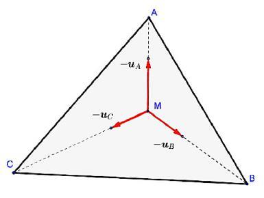
E XAMPLE 1.2.–Considerinaplanethreepoints A, B and C .Wewishtofindapoint M intheplanesuchthat l (M ) ≡ MA + MB + MC isofminimumlength.
Giventhat l (M ) iscontinuousandgreaterthanzero,thelength l (M ) doesadmit alowerlimit.Giventhatitispossibletolimitourselvestoacompactdomaininthe plane(suchasthedomainboundedbyadiskwhoseradiusissufficientlylarge),the minimumisobtained.
Letuscalculatethevariationdenotedby δl (M ): δl (M ) ≡ δMA + δMB + δMC . Wefirstcompute δMA;letuscarryoutthecalculususingorthonormalaxeswhose originis A;for M withthecoordinates x and y , r = MA = x2 + y 2 .Wederive
δMA = x x2 + y 2 δx + y x2 + y 2 δy =grad r δx δy where gradr= uA with uA =
Thebipoint AM correspondstothevectoroftail A andhead M .Thecomputation iscarriedoutinthesamewayforthepoints B and C ,andweobtain
δl (M )=0 ⇐⇒ uA + uB + uC = 0.
Thepoint M belongstothearcthatisabletosupport AB withtheangle 2 3 π .This isthesamefor BC andfor AC .Inorderforthearcstohaveacommonpoint,itis essentialthat |ABC | < 2 3 π ;noangleintriangleABCcanbelargerthan 2 3 π .The processforfindingthepointMisrepresentedinFigure1.1.
InthecasewhereoneoftheverticesintriangleABCcanhaveananglegreaterthan 2 3 π ,thepoint M cannotbefoundatanypointintheplaneexcept A, B or C .Indeed, weknowthatanextremumexistsandthat A, B and C arethepointsforwhich l (M ) isnotdifferentiable;atthesepoints,thecalculusgivenaboveisnotvalid.Itmustalso benotedthatthereexistsasinglesolutionandthissinglesolutionisaminimum.
Figure1.1. Representationofthetriangle ABC inthecasewherenovertexcanhave ananglegreaterthanorequalto 2 3 π .Thepoint M correspondstotheminimum distance MA + MB + MC .Foracolorversionofthefiguresinthischapter,see www.iste.co.uk/gouin/mechanics.zip
1.2.Firstconstrainedextremumproblem–Lagrangemultipliers
1.2.1. ExampleofLagrangemultiplier
T HEOREM 1.1.–Let A bealinearmappingfrom Rn to Rq andlet B bealinear mappingfrom Rn to Rp .Regardlessofthevector V in Rn , B V =0 implies AV =0 isequivalent:thereexistsalinearmapping Λ,from Rp to Rq ,calledtheLagrange multipliersuchthat A =ΛB
P ROOF.–Asthepropertyisanequivalence,itmustbeformulatedasanecessaryand sufficientcondition.
⇐ If V ∈ Ker B ,then ΛB V =0 and V ∈ Ker A
⇒ Reciprocally,assumethat Ker A⊂ Ker B , Ker A beingavectorsub-space of Rn .Thereexistsanadditionalvectorsub-spaceEof Ker B suchthat Rn =Ker B E .Thus, B|E isanisomorphismfromEtoIm B⊂ Rp andis invertible;and B|E 1 isalinearmappingfromIm B to E .Letuswrite Λ1 = A B|E 1 ,amappingfromIm B to Rq .Wecanwrite Rp = Im B E , where E isanadditionalvectorspaceofIm B relativeto Rp .Let Λ2 beanarbitrary linearmappingover E (wecanconsider,forexample,thelinearmappingwithzero values).Thus,
∀ V , V ∈ Rp , V = V 1 + V 2
Thisdecompositionisunique.Letuspositthat Λ isalinearmappingfrom Rp to Rq suchthat Λ(V )=Λ1 (V 1 )+Λ2 (V 2 ).Therefore, A =ΛB .Indeed,forany W , beingavectorin Rn ,itispossibletowrite W = W 1 + W 2 ,where W 1 ∈ Ker B and W 2 ∈ E ,thedecompositionbeingunique.Ontheonehand, A B|E 1 B (W 1 + W 2 )= A(W 2 ) since B|E 1 B istheidentityover E and B (W 1 )=0.Onthe otherhand, A(W )= A(W 1 + W 2 )= A(W 1 )+ A(W 2 ) and Ker A⊂ Ker B impliesforany W 1 ∈ Ker A, A(W )= A(W 2 ).Finally,foranyvector W in Rn , A(W )=ΛB (W ),i.e. A =ΛB .
1.2.2. Applicationtotheconstrainedextremumproblem
Let G beadifferentiablemappingfrom Rn to R and F beanotherdifferentiable mappingfrom Rn to Rp .Wewishtofindvaluesfortheelement x belongingto Rn suchthat a = G(x) beanextremum,knowingthat x satisfiesthecondition F (x)= 0 (called aconstraint ).Wemustwrite: δa =0 notforall δ x butforall δ x verifyingthe condition F (x) δ x =0.Wewrite,
∀ δ x, δ x ∈ Rn ,F (x) δ x = 0 =⇒ G (x) δ x =0 with F (x)=0,
Onthebasisof Rn and Rp ,letuswrite F usingcolumnmatrices x =
x1 . xn
1 (x1 ,...,xn ) . fp (x1 ,...,xn )
∈ Rp and F (x)=0 ⇐⇒
p (x1 ,...,xn )=0 .
TheJacobianmatrixofthe derivative of F (x) isrepresentedby
1 (x1 ,...,xn ) ∂x1 ,...,
F (x)=
1 (x1 ,...,xn )
n . . . .
p (x1 ,...,xn )
1 ,...,
p (x1 ,...,xn )
Thecondition F (x) δ x = 0 iswritteninmatrixformas
∂f1 (x1 ,...,xn )
∂x1 ,...,
∂f1 (x1 ,...,xn ) ∂xn . . . . . .
∂fp (x1 ,...,xn )
∂x1 ,..., ∂fp (x1 ,...,xn ) ∂xn
wherethefinalcolumnismadeupof p lines.
Theconditionfortheextremumof G canthenbewritteninmatrixformas
∂G(x1 ,...,xn )
∂x1 ,..., ∂G(x1 ,...,xn )
ApplyingTheorem1.1,thereexistsaLagrangemultiplier Λ,whichisalinear mappingfrom Rp to R suchthat
G (x)=Λ F (x)with F (x)=0.
Onthebasisof Rp ,wewrite
Λ=[λ1 ,...,λp ] or λi ∈ R,i ∈{1,...,p}
Thefollowingthreepropertiesareequivalent:
(A) ∀ δ x, δ x ∈ Rn ,F (x) δ x = 0 =⇒ G (x)δ x =0 with F (x)= 0;
(B) G (x)=Λ F (x) with F (x)= 0;
(C) ∀ δ x,δ x ∈ Rn and ∀ δ Λ,δ Λ ∈L(Rn , R),δ [G(x) Λ F (x)]=0.
Wehavedemonstratedthat (A) isequivalentto (B).Property (C) showsthatfinding aconnectedextremumisthesameasfindingafreeextremum,butwithrespectto n + p variables,thepositionoftheextremumbeingmadeupoftheelements x and Λ. TheintroductionofaLagrangemultiplierleadstothefreeingoftheconstraint.This propertyresultsfromTheorem1.1,andwecanwritethat G(x) Λ F (x)= b,where b isthenewfunctiontostationarize.
1.3.Thefundamentallemmaofthecalculusofvariations
Inthecasewheretheunknownisanelementofafunctionalspace,wearetruly dealingwiththecalculusofvariations–thisisanextensionofdifferentialcalculus. Indeed,intheprecedingsections,wehaveusedthefollowinglemma:
Given A belongingto L(Rn , R),forany V belongingto Rn , AV =0 implies A = 0.
Itispossibletoproposethefollowinggeneralization:
Letusconsider E ,thesetof p-timedifferentiablerealfunctionsdefinedby
[t0 ,t1 ] ⊂ R −→ ψ (t) ∈ Rn .
If p =0,functionsaresimplycontinuous.Wemayadd ψ (t0 )= 0 and ψ (t1 )= 0. Theset E hasthestructureofarealvectorspace.Let φ beamapping
[t0 ,t1 ] ⊂ R −→ φ(t) ∈L(Rn , R) ≡ Rn , then φ,definedfrom R tothedualof Rn ,isassumedtobecontinuousover [t0 ,t1 ].
Letuswrite G (ψ )= ˆ t1 t0 φ(t)ψ (t)dt.Thismappingdefinedover E islinearasfor allscalars λ1 ,λ2 andforallfunctions ψ1 ,ψ2 ,
L EMMA 1.1.–Let φ beacontinuousmappingfrom [t0 ,t1 ] to L(Rn , R) and ψ a continuousmappingfrom [t0 ,t1 ] to Rn ;then,
Foranyψ, ˆ t1 t0 φ(t) ψ (t)dt =0 impliesφ = 0
P ROOF.–Itisenoughtodemonstratethelemmafor n =1.Letusassumethrough reductioadabsurdum thatthereexists t2 ∈ ]t0 ,t1 [ suchthat φ(t2 ) =0 (e.g.the φ(t2 ) valueisstrictlypositive).Since φ(t) iscontinuous,thereexists [t2 ,t3 ] includedin ]t0 ,t1 [ suchthatfor t belongingto [t2 ,t3 ] ,φ(t) > 0. Bychoosing ψ (t)=[(t t2 )(t3 t)]p+1 for t ∈ [t2 ,t3 ] and ψ (t)=0 for t/ ∈ [t2 ,t3 ],wewould have
ˆ t1 t0
φ(t)ψ (t)dt = ˆ t3 t2 φ(t)[(t t2 )(t3 t)]p+1 dt> 0,
whichleadstoacontradiction.Thislemmacaneasilybeextendedwhen t2 takesthe valueofoneofitslimits t0 or t1 andcanbeappliedinthecasewhere ψ (t0 )= ψ (t1 )=0 (aswasthecaseintheproof).
L EMMA 1.2.– duBois-Raymond’slemma. φ beingacontinuousmappingfrom [t0 ,t1 ] to L(Rn , R) and ψ beinganapplicationwithacontinuousderivativefrom [t0 ,t1 ] to Rn suchthat ψ (t0 )= ψ (t1 )= 0;then,
Foranyψ, ˆ t1 t0 φ(t) ψ (t) dt =0 impliesφ = C , where C isaconstantlinearmappingfrom Rn to R.
Then, ψ belongsto D1 [t0 ,t1 ]
P ROOF.–Itisenoughtodemonstratethelemmafor n =1;thiscaneasilybe extendedto n> 1.Letthereal c definedby ˆ t1 t0 (φ(t) c) dt =0.Letuswrite
ψ (t)= ˆ t t0 (φ(u) c) du. Wehave ψ (t) ∈ D1 [t0 ,t1 ].Accordingtothehypotheses, ˆ t1 t0
(t) c) ψ (t) dt =
(t1 ) ψ (t0 ))=0
However, ψ (t)= φ(t) c;hence, ˆ t1 t0 (φ(t) c)2 dt =0,whichimplies φ(t)= c
Letusnotethatwehavewritten G (ψ )= ˆ t1 t0
φ(t) ψ (t) dt; G isalinearmapping from E to R;consequently, G isalinearfunctionalof E oranelementinthedual vectorspace E ∗ .Theparallelwithsection1.2iscomplete.
1.4.Extremumofafreefunctional
Let G beacontinuouslydifferentiablemappingfrom Ω × [t0 ,t1 ] to R,with Ω ⊂ Rn .Thismappingisdenotedby
(Q,t) ∈ Ω × [t0 ,t1 ] −→ G(Q,t) ∈ R andwesaythatGisa generatingfunction.Let φ beacontinuousmappingfrom [t0 ,t1 ] to Rn .Weposit
a = ˆ t1
G(φ(t),t)dt,
t0
andwewrite a = G (φ);thus, G isafunctionalofthe φ-functionsandbelongsto A(A(R, Rn ), R)
Let ψ beanothercontinuousmappingfrom [t0 ,t1 ] to Rn .Asthescalar x isreal, φ + xψ isacontinuousapplicationfrom [t0 ,t1 ] to Rn and
G (φ + xψ )= ˆ t1 t0 G φ(t)+ xψ (t),t dt.
Forthegiven φ and ψ ,wewrite g (x)= G (φ + xψ ).Thus,themapping g isalinear mappingfrom R to R.Forthegiven φ, ψ and t,wewrite f (x)= G φ(t)+ xψ (t),t . Thefunction f canbederivedat x =0,i.e.
f (x)= f (0)+ xf (0)+ xε(x) where lim x→0 ε(x)=0. Consequently,as ∂G φ(t),t ∂ Q isalinearmappingfrom Rn to R,
(x)= G
)+
Q φ(t),t ψ (t) +x ψ (t) ε xψ (t) , where lim x→0
xψ (t) =0, and,throughintegration
OROLLARY 1.1.–
whichcorrespondstothederivativeof g at 0.
(t),t
(t)dt + xε1 (x),
D EFINITION 1.2.– a = ˆ t1 t0 G φ(t),t dt isanextremumforthecontinuousfunction
φ from [t0 ,t1 ] to Rn ifandonlyifforany ψ continuousmappingfrom [t0 ,t1 ] to Rn ,
g (0) ≡ ˆ t1 t0 ∂G
(t)dt =0.
Wewrite δa = g (0),whichiscalled thevariationof a relativetothecontinuous functions φ from [t0 ,t1 ] to Rn .Whenthereisnoambiguity,wewrite
a = ˆ t1 t0 G(Q,t) dt, and,analogouswiththeprevioussections, ψ (t) isdenotedby δ Q(t) or,moresimply, δ Q Wewrite
g (0)= δa = ˆ t1
FromLemma1.2andCorollary1.1,itfollowsthat
C OROLLARY 1.2.– a = ˆ t1 t0 G Q,t dt isanextremumforthecontinuousfunction
Q from [t0 ,t1 ] to Rn if ∂G(Q,t) ∂ Q = 0.
Whenthereisnoambiguity,wewrite ∂G ∂Q for ∂G(Q,t) ∂Q .
1.5.Extremumforaconstrainedfunctional
Thesearchforthefunction t ∈ [t0 ,t1 ] −→ φ(t) ∈ Rn maysatisfycertain relationshipscalledconstraints.Wecomeacrosstwotypesofconstraints.
1.5.1. Firsttype:integralconstraint
D EFINITION 1.3.–Anintegralconstraintisarelationshipintheform
ˆ t1 t0 F (φ(t),t) dt = b, [1.1]
where b isagivenrealand F isacontinuouslydifferentiablemappingfromanopen set Ω of Rn × [t0 ,t1 ] to R.
Wecangeneralizethedefinitionforamappingfrom Rn × [t0 ,t1 ] to Rp .The generalizationcorrespondsto p integralconstraints.Findingthemappings φ which willmake ˆ t1 t0 G(φ(t),t)dt extremumandwhicharesubjecttocondition[1.1]results intheshortenedform:
∀ ψ continue,ψ ∈A(R, Rp ),
≡
,t
Wecansimplywrite: δb =0=⇒ δa =0.
(t)dt =0.
T HEOREM 1.2.–With δb and δa beingtwolinearfunctionalsdefinedoverthe continuousmappings φ from R to Rn ,withvaluesin R, δb =0=⇒ δa =0
isequivalenttothereexistingaLagrangemultiplier,i.e.alinearmappingfrom R to R suchthat δa = λδb.Wecanwrite
t1 t0
Q (φ(t),t) ψ
Thus, λ isarealconstant.
Wearebroughtbacktothesearchforthefreeextremumof
Lemma1.1ofthecalculusofvariationsimpliesthefollowingtheorem.
T HEOREM 1.3.–Thecontinuousfunctions φ from [t0 ,t1 ] to Rn ,satisfying relationship[1.1]andwhichmakes“integral a”extremum,simultaneouslysatisfythe tworelations:
Wealsousetheresultinsimplifiedformas
Q (Q(t),t)= λ ∂F
Thesepropertiesgeneralize,forfunctionalswithrealvalues,theresultsobtained insection1.4.
P ROOF.–Wedemonstratethepropertyinthecaseofamapping φ from R to R.We caneasilygeneralizethedemonstrationtothemappingswithvaluesin Rn .Letus write a = ˆ t1
(x(t),t)dt and b = ˆ
(x(t),t)dt,
where f and g aretwocontinuouslydifferentiablemappingsfrom R2 to R and x(t) denotesacontinuousmappingfrom R to R.Thus, δa = ˆ t1 t0 ∂g ∂x (x(t),t)δxdt and δb =
(x(t),t)δxdt.
Letuswrite J (δx)= ˆ t1 t0 ∂g ∂x (x(t),t) δxdt and K (δx)= ˆ t1 t0 ∂f ∂x (x(t),t) δxdt.
Theterms J and K aretwolinearmappingsdefinedover δx mappingsfrom R to R.Thus,
∀ δx,δx ∈ C 0 (R, R), K (δx)=0=⇒J (δx)=0
Let δx1 beagivencontinuousmappingfrom R to R suchthat K (δx1 ) =0 and δx isanyothercontinuousmappingfrom R to R.Letuswrite δx2 = δx μδx1 , where μ ∈ R andsuchthat K (δx2 )=0.Thisimpliesthat K (δx μδx1 )=0 or μ = K (δx)/K (δx1 ) ∈ R.Accordingtothehypothesis,weobtain K (δx2 )=0=⇒ J (δx2 )=0.Fromthisresult,itcanbederivedthat
J (δx2 )= J (δx) μ J (δx1 )=0=⇒J (δx2 ) = J (δx) −K (δx) J (δx1 ) K (δx1 ) =0
Letuswrite λ = J (δx1 )/K (δx1 ); λ isascalarthatisgivenby δx1 .Hence, J (δx)= λ K (δx)
C OROLLARY 1.3.–Thethreepropositionsareequivalent:
(A) ∀ δx, K (δx)=0=⇒J (δx)=0;
(B ) ∃ λ ∈ R suchthat ∀ δx,δx ∈ C 0 (R, R), J (δx) λ K (δx)=0;
(C ) ∃ λ ∈ R, aconstantscalar,calledtheLagrangemultiplier,suchthat
J = λ K
Wealsowrite δa λδb =0.
1.5.2. Secondtype:distributedconstraint
Let F beamappingfrom Ω × [t0 ,t1 ] to R,where Ω isanopensetof Rn and [t0 ,t1 ] asegmentof R.Wewishtofindtheextremaof a = ˆ t1 t0 G(Q(t),t)dt suchthat,for anyvalue t of [t0 ,t1 ],wehave F (Q(t),t)=0.Theconstraint F (Q(t),t)=0 is calledadistributedconstraint.
Wedemonstratethatweareledtointroduceamultiplierdenotedby Λ,afunction definedforeachvalueof t belongingto [t0 ,t1 ],i.e.a Λ-multiplierfunctionof t.
T HEOREM 1.4.–Wehavetheequivalenceofthethreepropositions:
(A)thereexistsacontinuousmapping Q from [t0 ,t1 ] to Ω satisfying F (Q(t),t)=0 suchthatforanycontinuousapplication δ Q from [t0 ,t1 ] to Rn and forany t of [t0 ,t1 ],
∂F
∂ Q (Q(t),t) δ Q =0=⇒ δ ˆ t1 t
(Q(t),t)dt =0;
(B)thereexistsacontinuousmapping Q from [t0 ,t1 ] to Ω andthereexistsa continuousmapping Λ from [t0 ,t1 ] to R suchthatforanycontinuousmapping δ Q from [t0 ,t1 ] to Rn andanycontinuousmapping δ Λ from [t0 ,t1 ] to R, δ ˆ t1 t0 G(Q(t),t) Λ(t) F (Q(t),t) dt =0;
(C)thereexistsacontinuousmapping Q from [t0 ,t1 ] to Ω andthereexistsa continuousmapping Λ from [t0 ,t1 ] to R suchthat ∂G
∂ Q (Q(t),t) Λ(t) ∂F ∂Q (Q(t),t)=0 and F (Q(t),t)=0