Preface to the Ninth Edition
In presenting this new edition of Kanski’s Clinical Ophthalmology, I am reminded of a quotation from Lewis Carroll’s Alice’s Adventures in Wonderland: “What is the use of a book”, thought Alice, “without pictures or conversations?”. The ninth edition of this classic textbook is filled with beautiful illustrations and considerable information and is intended to be a useful and comprehensive basis for general ophthalmic practice. It has been a privilege to work on this remarkable book and I am grateful to Jack Kanski and the staff of Elsevier for entrusting me with the task.
The challenge has been to cover the entire field of ophthalmology for a worldwide audience without depending on subspecialists to prepare each chapter. In order to do this, I have maintained Jack Kanski’s unique approach of presenting core clinical knowledge in a systemic and succinct form. Brad Bowling has had a significant influence on the two previous editions and his accuracy and meticulous attention to detail has been extremely helpful. I have reverted to the format that was used in the sixth edition by starting with an initial chapter on examination techniques. Special investigations remain in the chapters where they are most relevant. Each chapter has been updated and the latest evidence-based diagnostic and therapeutic approaches have been covered, including genetics, immunotherapy and imaging techniques. Many new illustrations have been added and better examples of a range of conditions have been used. Jack Kanski’s idea of including important ‘tips’ has been reintroduced. I have included sufficient practical information for trainees to manage common ophthalmic conditions in the clinic and enough detail on rare conditions to enable them to prepare for their examinations without resorting to the internet.
I have been extremely fortunate to have received help from colleagues past and present, to whom I wish to express my grateful thanks. The photographers and research staff at the Oxford Eye Hospital have been wonderfully supportive. Jack Kanski generously gave me his huge collection of images. My friends in
South Africa, Tony Murray (strabismus) and Trevor Carmichael (cornea), provided help with the text and images of pathology that are not easily found in developed countries. I received many pictures from Jonathan Norris and Elizabeth Insull (oculoplastics), Darius Hildebrand and Manoj Parulekar (paediatrics), Peter Issa and Christine Kiire (medical retina), Bertil Damato (ocular oncology), Martin Leyland (corneal surgery), C.K. Patel (vitreoretinal surgery), Patsy Terry (ultrasound) and Pieter Pretorius (neuroradiology). Mitch Ménage provided good pictures of common conditions. Aude Ambresin and Carl Herbort (Switzerland) supplied state-of-the-art retinal images. I have kept many of the outstanding pictures that Chris Barry and Simon Cheng (Australia) provided for the eighth edition. Single examples of rare conditions have been kindly provided by a number of colleagues throughout the United Kingdom and elsewhere and their contribution has been recognized next to the images provided. Other individuals have helped substantially with previous editions of Clinical Ophthalmology, including Terry Tarrant, the artist who produced the meticulous ocular paintings. I also wish to thank Kim Benson, Sharon Nash, Kayla Wolfe, Julie Taylor, Anne Collett and the production team at Elsevier.
The ninth edition of Kanski’s Clinical Ophthalmology could not have been produced in the time available without the help of my assistant, Carolyn Bouter, whose resilience, diligence, intelligence and skill were evident throughout the 6 months that she worked with me. I have also had the good fortune to work with Jonathan Brett, a world-class photographer and artist, whose genius is present in hundreds of the images included in this edition. My wife, Susie, has been extremely supportive throughout this project and her happy and helpful nature has made the task a pleasant and enjoyable experience.
John F. Salmon 2019
AAION arteritic anterior ischaemic optic neuropathy
AAU acute anterior uveitis
AC anterior chamber
AC/A ratio accommodative convergence/accommodation ratio
ACE angiotensin converting enzyme
AD autosomal dominant
AF autofluorescence
AGIS Advanced Glaucoma Treatment Study
AHP abnormal head posture
AI accommodative insufficiency
AIBSE acute idiopathic blind spot enlargement syndrome
AIDS acquired immune deficiency syndrome
AIM (unilateral) acute idiopathic maculopathy
AION anterior ischaemic optic neuropathy
AIR autoimmune retinopathies
AKC atopic keratoconjunctivitis
ALT argon laser trabeculoplasty
AMD age-related macular degeneration
AMN acute macular neuroretinopathy
ANA antinuclear antibody
ANCA antineutrophil cytoplasmic antibodies
APD afferent pupillary defect
APMPPE acute posterior multifocal placoid pigment epitheliopathy
AR autosomal recessive
AREDS Age-Related Eye Disease Study
ARN acute retinal necrosis
ARPE acute retinal pigment epitheliitis
AZOOR acute zonal occult outer retinopathy
AZOR acute zonal outer retinopathy
BADI bilateral acute depigmentation of the iris
BCC basal cell carcinoma
BCVA best-corrected visual acuity
BIO binocular indirect ophthalmoscopy
BP blood pressure
BRAO branch retinal artery occlusion
BRVO branch retinal vein occlusion
BSV binocular single vision
BUT breakup time
CAI carbonic anhydrase inhibitor
CCDD congenital cranial dysinnervation disorders
CCT central corneal thickness
C/D cup/disc
CDCR canaliculodacryocystorhinostomy
CF counts (or counting) fingers
CHED congenital hereditary endothelial dystrophy
CHP compensatory head posture
CHRPE congenital hypertrophy of the retinal pigment epithelium
CI convergence insufficiency
Abbreviations
C-MIN conjunctival melanocytic intraepithelial neoplasia
CMO cystoid macular oedema (US = CME)
CNS central nervous system
CNV choroidal neovascularization
CNVM choroidal neovascular membrane
COX-2 cyclo-oxygenase-2
CPEO chronic progressive external ophthalmoplegia
CRAO central retinal artery occlusion
CRP C-reactive protein
CRVO central retinal vein occlusion
CSC central serous chorioretinopathy
CSC/CSCR central serous chorioretinopathy
CSMO clinically significant macular oedema (US = CSME)
CSR central serous chorioretinopathy
CSS central suppression scotoma
CT computed tomography
CXL corneal collagen cross-linking
DALK deep anterior lamellar keratoplasty
DCCT Diabetes Control and Complication Trial
DCR dacryocystorhinostomy
DCT dynamic contour tonometry
DMEK Descemet membrane endothelial keratoplasty
DMO diabetic macular oedema (US = DME)
DR diabetic retinopathy
DRCR.net Diabetic Retinopathy Clinical Research Network
DRPPT dark room prone provocative test
DRS Diabetic Retinopathy Study
DSAEK Descemet stripping automated endothelial keratoplasty
DVD dissociated vertical deviation
ECG electrocardiogram
EDTA ethylenediaminetetraacetic acid
EGFR epidermal growth factor inhibitors
EKC epidemic keratoconjunctivitis
EMGT Early Manifest Glaucoma Trial
EOG electro-oculography/gram
ERG electroretinography/gram
ERM epiretinal membrane
ESR erythrocyte sedimentation rate
ETDRS Early Treatment Diabetic Retinopathy Study
ETROP Early Treatment of Retinopathy of Prematurity
FA fluorescein angiography (also FFA)
FAF fundus autofluorescence
FAP familial adenomatous polyposis
FAZ foveal avascular zone
FBA frosted branch angiitis
FBC full blood count
FDT frequency doubling test
FFM fundus flavimaculatus
FTMH full-thickness macular hole
5-FU 5-fluorouracil
GA geographic atrophy
GAT Goldmann applanation tonometry
GCA giant cell arteritis
GDD glaucoma drainage device
GHT glaucoma hemifield test
GPA guided progression analysis
GPC giant papillary conjunctivitis
G-TOP glaucoma tendency orientated perimetry
HAART highly active antiretroviral therapy
HFA Humphrey field analyser
HIV human immunodeficiency virus
HM hand movements
HRT Heidelberg retinal tomography
HSV-1 herpes simplex virus type 1
HSV-2 herpes simplex virus type 2
HZO herpes zoster ophthalmicus
ICE iridocorneal endothelial
ICG indocyanine green
ICGA indocyanine green angiography
ICROP International Classification of Retinopathy of Prematurity
IFIS intraoperative floppy iris syndrome
Ig immunoglobulin
IK interstitial keratitis
ILM internal limiting membrane
IMT idiopathic macular telangiectasia
INO internuclear ophthalmoplegia
INR international normalized ratio
IOFB intraocular foreign body
IOID idiopathic orbital inflammatory disease
IOL intraocular lens
IOP intraocular pressure
IRMA intraretinal microvascular abnormality
IRVAN idiopathic retinal vasculitis, aneurysms and neuroretinitis syndrome
ITC iridotrabecular contact
IU intermediate uveitis
IVTS International Vitreomacular Traction Study
JIA juvenile idiopathic arthritis
KC keratoconus
KCS keratoconjunctivitis sicca
KP keratic precipitate
LA local anaesthetic
LASEK laser (also laser-assisted) epithelial keratomileusis
LASIK laser-assisted in situ keratomileusis
LN latent nystagmus
LSCD limbal stem cell deficiency
LV loss variance
MALT mucosa-associated lymphoid tissue
MCP multifocal choroiditis and panuveitis
MEWDS multiple evanescent white dot syndrome
MFC multifocal choroiditis and panuveitis
MIGS minimally invasive glaucoma surgery
MLF medial longitudinal fasciculus
MLT micropulse laser technology
MMC mitomycin C
MPS mucopolysaccharidosis
MRI magnetic resonance imaging
MS multiple sclerosis
NF1 neurofibromatosis type I
NF2 neurofibromatosis type II
NPDR non-proliferative diabetic retinopathy
NRR neuroretinal rim
NSAID non-steroidal anti-inflammatory drug
NSR neurosensory retina
NTG normal-tension glaucoma
NVD new vessels on the disc
NVE new vessels elsewhere
NVG neovascular glaucoma
NVI new vessels iris
OCT optical coherence tomography/gram
OHT ocular hypertension
OHTS Ocular Hypertension Treatment Study
OIS ocular ischaemia syndrome
OKN optokinetic nystagmus
OVD ophthalmic viscosurgical devices
PAC primary angle closure
PACG primary angle-closure glaucoma
PACS primary angle-closure suspect
PAM primary acquired melanosis
PAN polyarteritis nodosa
PAS peripheral anterior synechiae
PC posterior chamber
PCO posterior capsular opacification
PCR polymerase chain reaction
PCV polypoidal choroidal vasculopathy
PDR proliferative diabetic retinopathy
PDS pigment dispersion syndrome
PDT photodynamic therapy
PED pigment epithelial detachment
PEE punctate epithelial erosions
PEK punctate epithelial keratitis
PEHCR peripheral exudative haemorrhagic chorioretinopathy
PH pinhole
PHM posterior hyaloid membrane
PIC punctate inner choroidopathy
PIOL primary intraocular lymphoma
PION posterior ischaemic optic neuropathy
PKP penetrating keratoplasty
PMMA polymethyl methacrylate
POAG primary open-angle glaucoma
POHS presumed ocular histoplasmosis syndrome
PP pars planitis
PPCD posterior polymorphous corneal dystrophy
PPDR preproliferative diabetic retinopathy
PPM persistent placoid maculopathy
PPRF paramedian pontine reticular formation
PPV pars plana vitrectomy
PRK photorefractive keratectomy
PRP panretinal photocoagulation
PS posterior synechiae
PSD pattern standard deviation
PSS Posner-Schlossman syndrome
PUK peripheral ulcerative keratitis
PVD posterior vitreous detachment
PVR proliferative vitreoretinopathy
PVRL primary vitreoretinal lymphoma
PXE pseudoxanthoma elasticum
PXF pseudoexfoliation
RA rheumatoid arthritis
RAO retinal artery occlusion
RAPD relative afferent pupillary defect
RD retinal detachment
RNFL retinal nerve fibre layer
ROCK Rho-kinase
ROP retinopathy of prematurity
RP retinitis pigmentosa
RPC relentless placoid chorioretinitis
RPE retinal pigment epithelium
RRD rhegmatogenous retinal detachment
RS retinoschisis
RVO retinal vein occlusion
SANS space flight-associated neuro-ocular syndrome
SAP standard automated perimetry
SCC squamous cell carcinoma
SCN suprachiasmic nucleus
SD-OCT spectral domain optical coherence tomography
SF short-term fluctuation
SFU progressive subretinal fibrosis and uveitis syndrome
SIC solitary idiopathic choroiditis
SITA Swedish Interactive Thresholding Algorithm
SJS Stevens–Johnson syndrome
SLK superior limbic keratoconjunctivitis
SLT selective laser trabeculoplasty
SMILE small incision lenticule extraction
SPARCS Spaeth Richman contrast sensitivity test
SPK superficial punctate keratitis
SRF subretinal fluid
SS Sjögren syndrome
STIR short T1 inversion recovery
SWAP short-wave automated perimetry
TAL total axial length
TB tuberculosis
TEN toxic epidermal necrolysis
TGF transforming growth factor
TIA transient ischaemic attack
TM trabecular meshwork
TRD tractional retinal detachment
TRP targeted retinal photocoagulation
TTT transpupillary thermotherapy
UBM ultrasonic biomicroscopy
US ultrasonography
VA visual acuity
VEGF vascular endothelial growth factor
VEP visual(ly) evoked potential(s)
VFI visual field index
VHL von Hippel–Lindau syndrome
VKC vernal keratoconjunctivitis
VKH Vogt–Koyanagi–Harada syndrome
VMA vitreomacular adhesion
VMT vitreomacular traction
VZV varicella zoster virus
XL X-linked
Chapter 1 Examination Techniques
INTRODUCTION 2
PSYCHOPHYSICAL TESTS 2
Visual acuity 2
Near visual acuity 4
Contrast sensitivity 4
Amsler grid 5
Light brightness comparison test 6
Photostress test 6
Colour vision testing 7
Plus lens test 9
PERIMETRY 9
Definitions 9
Testing algorithms 11
Testing patterns 14
Analysis 14
High-sensitivity field modalities 17
Sources of error 18
Microperimetry 18
SLIT LAMP BIOMICROSCOPY OF THE ANTERIOR SEGMENT 20
Direct illumination 20
Scleral scatter 20
Retroillumination 20
Specular reflection 21
FUNDUS EXAMINATION 21
Direct ophthalmoscopy 21
Slit lamp biomicroscopy 22
Goldmann three-mirror examination 23
Head-mounted binocular indirect ophthalmoscopy 25
Fundus drawing 27
TONOMETRY 27
Goldmann tonometry 27
Other forms of tonometry 29
Ocular response analyser and corneal hysteresis 30
GONIOSCOPY 30
Introduction 30
Indirect gonioscopy 32
Direct gonioscopy 33
Identification of angle structures 34
Pathological findings 35
CENTRAL CORNEAL THICKNESS 36
INTRODUCTION
Patients with ophthalmic disease must have their vision accurately measured and their eyes need to be examined using specialized techniques. Special investigations should be used to supplement the findings of clinical examination. Electrophysical tests, fluorescein angiography and optical coherence tomography are discussed in later chapters.
PSYCHOPHYSICAL TESTS
Visual acuity
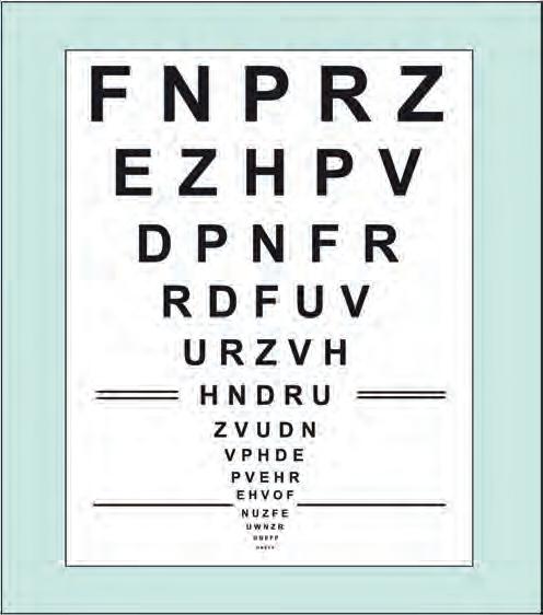
Snellen visual acuity
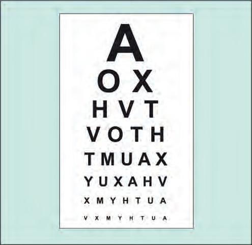
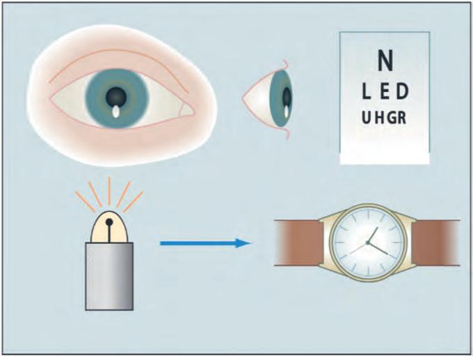
Distance visual acuity (VA) is directly related to the minimum angle of separation (subtended at the nodal point of the eye) between two objects that allow them to be perceived as distinct. In practice, it is most commonly carried out using a Snellen chart, which utilizes black letters or symbols (optotypes) of a range of sizes set on a white chart (Fig. 1.1), with the subject reading the chart from a standard distance. Distance VA is usually first measured using a patient’s refractive correction, generally their own glasses or contact lenses. For completeness, an unaided acuity may also be recorded. The eye reported as having worse vision should be tested first, with the other eye occluded. It is important to push the patient to read every letter possible on the optotypes being tested.
• Normal monocular VA equates to 6/6 (metric notation; 20/20 in non-metric ‘English’ notation) on Snellen testing. Normal corrected VA in young adults is often superior to 6/6.
• Best-corrected VA (BCVA) denotes the level achieved with optimal refractive correction.
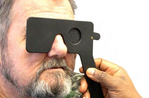
• Pinhole VA: a pinhole (PH) aperture compensates for the effect of refractive error, and consists of an opaque occluder perforated by one or more holes of about 1 mm diameter (Fig. 1.2). However, PH acuity in patients with macular disease and posterior lens opacities may be worse than with spectacle correction. If the VA is less than 6/6 Snellen equivalent, testing is repeated using a pinhole aperture.
• Binocular VA is usually superior to the better monocular VA of each eye, at least where both eyes have roughly equal vision.
Very poor visual acuity
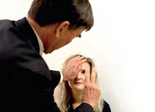
• Counting (or counts) fingers (CF) denotes that the patient is able to tell how many fingers the examiner is holding up at a specified distance (Fig. 1.3), usually 1 metre.
• Hand movements (HM) is the ability to distinguish whether the examiner’s hand is moving when held just in front of the patient.
• Perception of light (PL): the patient can discern only light (e.g. pen torch), but no shapes or movement. Careful occlusion of the other eye is necessary. If poor vision is due solely to a dense media opacity such as cataract, the patient should
Fig. 1.1 Snellen visual acuity chart
Fig. 1.2 Pinhole
Fig. 1.3 Testing of ‘counts fingers’ visual acuity
Fig. 1.4 Notation for the projection of light test (right eye); the patient cannot detect light directed from the superior and temporal quadrants
readily be able to determine the direction from which the light is being projected (Fig. 1.4).
LogMAR acuity
LogMAR charts address many of the deficiencies of the Snellen chart (Table 1.1), and are the standard means of VA measurement in research and, increasingly, in clinical practice.
• LogMAR is an acronym for the base-10 logarithm of the minimum angle of resolution (MAR) and refers to the ability to resolve the elements of an optotype. Thus, if a letter on the 6/6 (20/20) equivalent line subtends 5′ of arc, and each limb of the letter has an angular width of 1′, a MAR of 1′ is needed for resolution. For the 6/12 (20/40) line, the MAR is 2′, and for the 6/60 (20/200) line it is 10′
• The logMAR score is simply the base-10 log of the MAR. Because the log of the MAR value of 1′ is zero, 6/6 is equivalent to logMAR 0.00. The log of the 6/60 MAR of 10′ is 1, so 6/60 is equivalent to logMAR 1.00. The log of the 6/12 MAR of 2′ is 0.301, giving a logMAR score of 0.30. Scores better than 6/6 have a negative value.
• As letter size changes by 0.1 logMAR units per row and there are five letters in each row, each letter can be assigned a score of 0.02. The final score can therefore take account of every letter that has been read correctly and the test should continue until half of the letters on a line are read incorrectly.
LogMAR charts
• The Bailey–Lovie chart (Fig. 1.5).
○ Used at 6 m testing distance.
○ Each line of the chart comprises five letters and the spacing between each letter and each row is related to the width
Snellen LogMAR
Shorter test time
More letters on the lower lines introduces an unbalanced ‘crowding’ effect
Fewer larger letters reduces accuracy at lower levels of VA
Variable readability between individual letters
Lines not balanced with each other for consistency of readability
6 m testing distance: longer testing lane (or a mirror) required
Letter and row spacing not systematic
Lower accuracy and consistency so relatively unsuitable for research
Straightforward scoring system
Easy to use
Longer test time
Equal numbers of letters on different lines controls for ‘crowding’ effect
Equal numbers of letters on low and higher acuity lines increases accuracy at lower VA
Similar readability between letters
Lines balanced for consistency of readability
4 m testing distance on many charts: smaller testing lane (or no mirror) required
Letter and row spacing set to optimize contour interaction
Higher accuracy and consistency so appropriate for research
More complex scoring
Less user-friendly
Table 1.1 Comparison of Snellen and logMAR Visual Acuity Testing
Fig. 1.5 Bailey–Lovie chart
and the height of the letters. The letter signs are rectangular rather than square, as with the EDTRS chart. A 6/6 letter is 5′ in height by 4′ in width.
○ The distance between two adjacent letters on the same row is equal to the width of a letter from the same row, and the distance between two adjacent rows is the same as the height of a letter from the lower of the two rows.
○ Snellen VA values and logMAR VA are listed to the right and left of the rows respectively.
• The ETDRS (Early Treatment Diabetic Retinopathy Study) chart is calibrated for 4 m. This chart utilizes balanced rows comprising Sloan optotypes, developed to confer equivalent legibility between individual letters and rows. ETDRS letters are square, based on a 5 × 5 grid, i.e. 5′ × 5 ′ for the 6/6 equivalent letters at 6 m.
• Computer charts are available that present the various forms of test chart on display screens, including other means of assessment such as contrast sensitivity (see below).
TIP LogMAR charts are commonly used in clinical trials because they are the most accurate method of measuring VA.
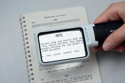
Near visual acuity
Near vision testing can be a sensitive indicator of the presence of macular disease. A range of near vision charts (including logMAR and ETDRS versions) or a test-type book can be used. The book or chart is held at a comfortable reading distance and this is measured and noted. The patient wears any necessary distance correction together with a presbyopia correction if applicable (usually their own reading spectacles). The smallest type legible is recorded for each eye individually and then using both eyes together (Fig. 1.6).
Contrast sensitivity
• Principles. Contrast sensitivity is a measure of the ability of the visual system to distinguish an object against its background.
A target must be sufficiently large to be seen, but must also be of high enough contrast with its background. A light grey letter will be less well seen against a white background than a black letter. Contrast sensitivity represents a different aspect of visual function to that tested by the spatial resolution tests described above, which all use high-contrast optotypes.
○ Many conditions reduce both contrast sensitivity and VA, but under some circumstances (e.g. amblyopia, optic neuropathy, some cataracts, and higher-order aberrations), visual function measured by contrast sensitivity can be reduced whilst VA is preserved.
○ Hence, if patients with good VA complain of visual symptoms (typically evident in low illumination), contrast sensitivity testing may be a useful way of objectively demonstrating a functional deficit. Despite its advantages, it has not been widely adopted in clinical practice.
• The Pelli–Robson contrast sensitivity letter chart is viewed at 1 metre and consists of rows of letters of equal size (spatial frequency of 1 cycle per degree) but with decreasing contrast of 0.15 log units for groups of three letters (Fig. 1.7). The patient reads down the rows of letters until the lowest-resolvable group of three is reached.
• Sinusoidal (sine wave) gratings require the test subject to view a sequence of increasingly lower contrast gratings.
• Spaeth Richman contrast sensitivity test (SPARCS) is performed on a personal computer with internet access. It can be accessed online. Each patient is supplied with an identification number and instructions on how to do the test. The test takes 5–10 minutes per eye and measures both central and peripheral contrast sensitivity. Since the test is based on gratings it can be used on illiterate patients.
Fig. 1.6 Near visual acuity using a magnifying lens
Fig. 1.7 Pelli–Robson contrast sensitivity letter chart
Amsler grid
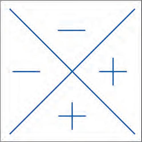
The Amsler grid evaluates the 20° of the visual field centred on fixation (Fig. 1.8). It is principally useful in screening for and monitoring macular disease, but will also demonstrate central visual field defects originating elsewhere. Patients with a substantial risk of choroidal neovascularization (CNV) should be provided with an Amsler grid for regular use at home.
TIP An Amsler grid is a simple and easy method of monitoring central visual field and is commonly abnormal in patients with macular disease.
Charts
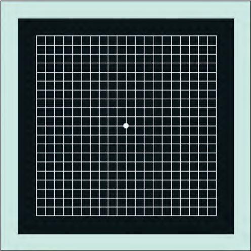
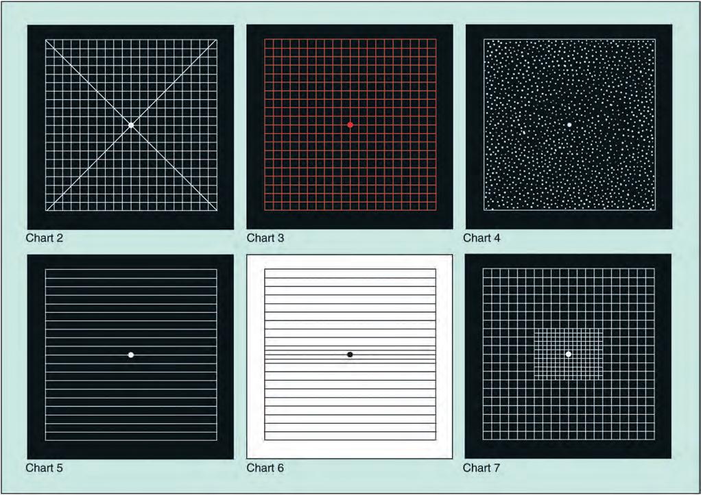
There are seven charts, each consisting of a 10-cm outer square (Figs 1.9 and 1.10).
• Chart 1 consists of a white grid on a black background, the outer grid enclosing 400 smaller 5-mm squares. When viewed at about one-third of a metre, each small square subtends an angle of 1°.
• Chart 2 is similar to chart 1 but has diagonal lines that aid fixation for patients with a central scotoma.
• Chart 3 is identical to chart 1 but has red squares. The red-onblack design aims to stimulate long wavelength foveal cones. It is used to detect subtle colour scotomas and desaturation in toxic maculopathy, optic neuropathy and chiasmal lesions.
• Chart 4 consists only of random dots and is used mainly to distinguish scotomas from metamorphopsia, as there is no form to be distorted.
• Chart 5 consists of horizontal lines and is designed to detect metamorphopsia along specific meridians. It is of particular use in the evaluation of patients describing difficulty reading.
• Chart 6 is similar to chart 5 but has a white background and the central lines are closer together, enabling more detailed evaluation.
• Chart 7 includes a fine central grid, each square subtending an angle of a half degree, and is more sensitive.
Technique
The pupils should not be dilated, and in order to avoid a photostress effect, the eyes should not yet have been examined on the slit lamp. A presbyopic refractive correction should be worn if appropriate. The chart should be well illuminated and held at a comfortable reading distance, optimally around 33 cm.
• One eye is covered.
• The patient is asked to look directly at the central dot with the uncovered eye, to keep looking at this, and to report any distortion or waviness of the lines on the grid.
• Reminding the patient to maintain fixation on the central dot, he or she is asked if there are blurred areas or blank spots anywhere on the grid. Patients with macular disease often report that the lines are wavy whereas those with optic neuropathy tend to remark that some of the lines are missing or faint but not distorted.
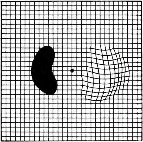
• The patient is asked if he or she can see all four corners and all four sides of the square – a missing corner or border should raise the possibility of causes other than macular disease, such as glaucomatous field defects or retinitis pigmentosa. The patient may be provided with a recording sheet and pen and asked to draw any anomalies (Fig. 1.11).
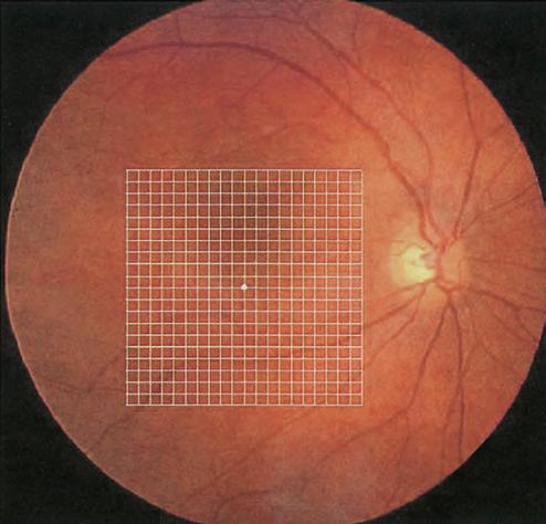
Fig. 1.8 Amsler grid superimposed on the macula. The central fixation dot of the grid does not coincide with the foveal anatomical centre in this image (Courtesy of A Franklin)
Fig. 1.9 Amsler grid chart (Courtesy of A Franklin)
Light brightness comparison test
This is a test of optic nerve function, which is usually normal in early and moderate retinal disease. It is performed as follows:
• A light from an indirect ophthalmoscope is shone first into the normal eye and then the eye with suspected disease.
• The patient is asked whether the light is symmetrically bright in both eyes.
• In optic neuropathy the patient will report that the light is less bright in the affected eye.
• The patient is asked to assign a relevant value from 1 to 5 to the brightness of the light in the diseased eye, in comparison to the normal eye.
Photostress test
• Principles. Photostress testing is a gross test of dark adaptation in which the visual pigments are bleached by light. This causes a temporary state of retinal insensitivity perceived by the patient as a scotoma. The recovery of vision is dependent on the ability of the photoreceptors to re-synthesize visual pigment. The test may be useful in detecting maculopathy
Fig. 1.10 Amsler charts 2–7 (Courtesy of A Franklin)
Fig. 1.11 Stylized Amsler recording sheet shows wavy lines indicating metamorphopsia, and a dense scotoma
when ophthalmoscopy is equivocal, as in mild cystoid macular oedema or central serous retinopathy. It may also differentiate visual loss caused by macular disease from that caused by an optic nerve lesion.
• Techniques
○ The best-corrected distance VA is determined.
○ The patient fixates on the light of a pen torch or an indirect ophthalmoscope held about 3 cm away for about 10 seconds (Fig. 1.12A).
○ The photostress recovery time (PSRT) is the time taken to read any three letters of the pre-test acuity line and is normally between 15 and 30 seconds (Fig. 1.12B).
○ The test is performed on the other, presumably normal, eye and the results are compared.
○ The PSRT is prolonged relative to the normal eye in macular disease (sometimes 50 seconds or more) but not in an optic neuropathy.
Colour vision testing
Introduction
Assessment of colour vision is useful in the evaluation of optic nerve disease and in determining the presence of a congenitally anomalous colour defect. Dyschromatopsia may develop in retinal dystrophies prior to the impairment of other visual parameters. Colour vision depends on three populations of retinal cones, each with a specific peak sensitivity: blue (tritan) at 414–424 nm, green (deuteran) at 522–539 nm and red (protan) at 549–570 nm. Normal colour perception requires all these primary colours to
match those within the spectrum. Any given cone pigment may be deficient (e.g. protanomaly – red weakness) or entirely absent (e.g. protanopia – red blindness). Trichromats possess all three types of cones (although not necessarily functioning perfectly), while absence of one or two types of cones renders an individual a dichromat or monochromat, respectively. Most individuals with congenital colour defects are anomalous trichromats and use abnormal proportions of the three primary colours to match those in the light spectrum. Those with red–green deficiency caused by abnormality of red-sensitive cones are protanomalous, those with abnormality of green-sensitive cones are deuteranomalous and those with blue–green deficiency caused by abnormality of bluesensitive cones are tritanomalous. Acquired macular disease tends to produce blue–yellow defects, and optic nerve lesions red–green defects.
Colour vision tests
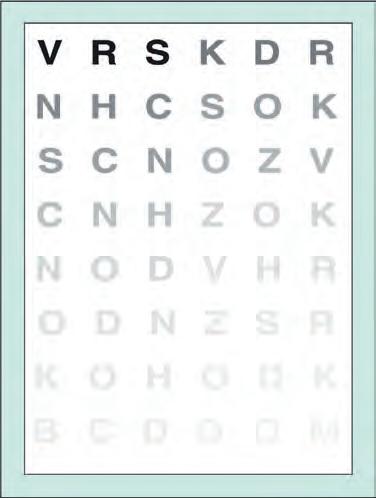
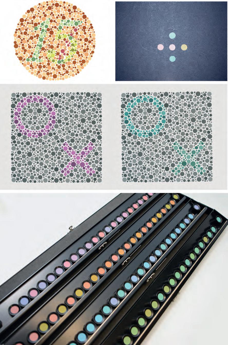
• The Ishihara test is designed to screen for congenital protan and deuteran defects. It is simple, widely available and frequently used to screen for a red–green colour vision deficit. The test can be used to assess optic nerve function. It consists of a test plate followed by 16 plates, each with a matrix of dots arranged to show a central shape or number that the subject is asked to identify (Fig. 1.13A). A colour-deficient person will only be able to identify some of the figures. Inability to identify the test plate (provided VA is sufficient) indicates non-organic visual loss.
• The City University test consists of 10 plates, each containing a central colour and four peripheral colours (Fig. 1.13B) from which the subject is asked to choose the closest match.
Fig. 1.12 Photostress test. (A) The patient looks at a light held about 3 cm away from the eye, for about 10 seconds; (B) the photostress recovery time is the time taken to read any three letters of the pre-test acuity line and is normally between 15 and 30 seconds
Fig. 1.13 Colour vision tests. (A) Ishihara; (B) City University; (C) Hardy–Rand–Rittler; (D) Farnsworth–Munsell 100-hue test
• The Hardy–Rand–Rittler test is similar to the Ishihara, but can detect all three congenital colour defects (Fig. 1.13C).
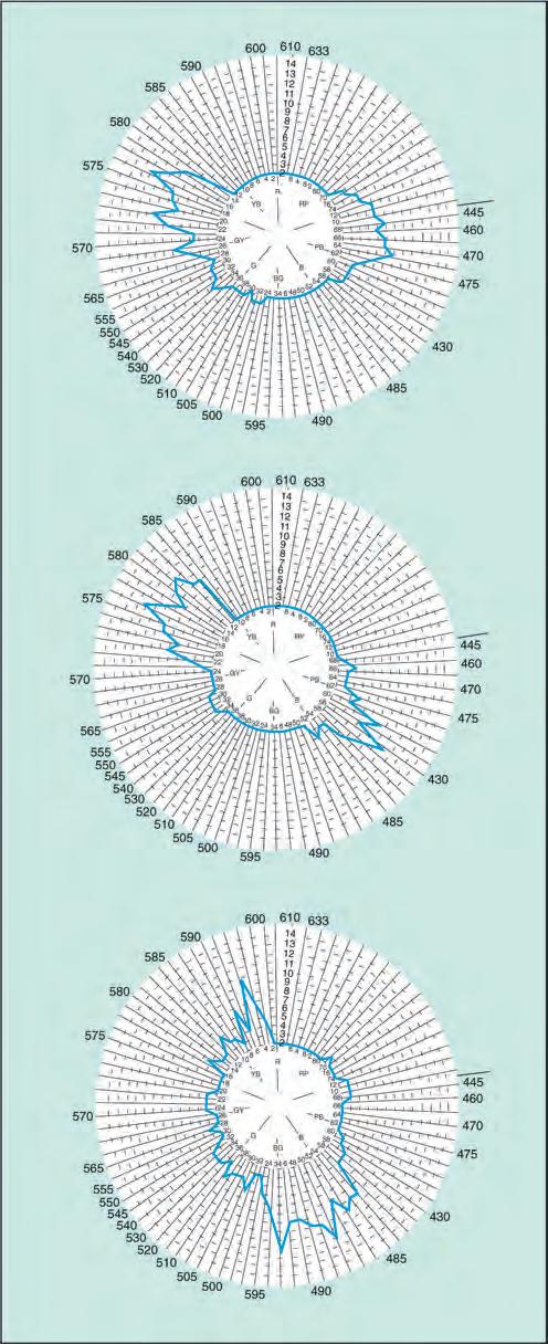
• The Farnsworth–Munsell 100-hue test is a sensitive but longer test for both congenital and acquired colour defects. Despite the name, it consists of 85 caps of different hues in four racks (Fig. 1.13D). The subject is asked to rearrange randomized caps in order of colour progression, and the findings are recorded on a circular chart. Each of the three forms of dichromatism is characterized by failure in a specific meridian of the chart (Fig. 1.14).
Plus lens test
A temporary hypermetropic shift may occur in some conditions due to an elevation of the sensory retina – the classic example is central serous chorioretinopathy (CSR). A +1.00-dioptre lens will demonstrate the phenomenon.
PERIMETRY
Definitions
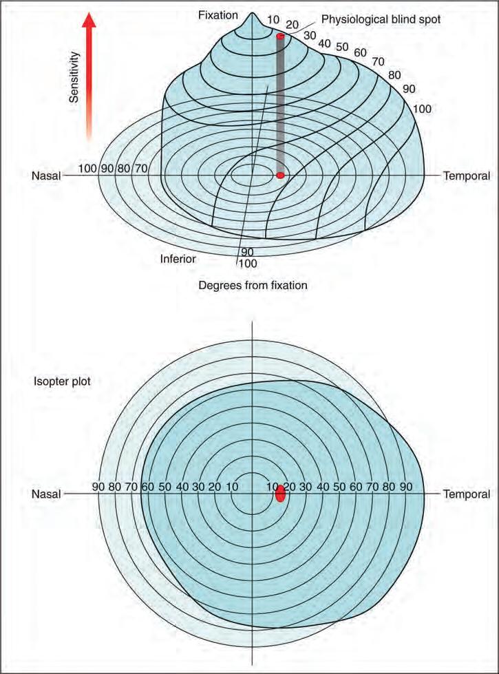
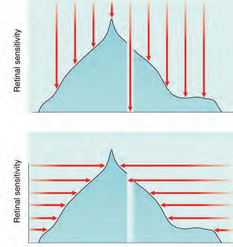
• The visual field can be represented as a three-dimensional structure akin to a hill of increasing sensitivity (Fig. 1.15A). The outer aspect extends approximately 50° superiorly, 60° nasally, 70° inferiorly and 90° temporally. VA is sharpest at the very top of the hill (i.e. the fovea) and then declines progressively towards the periphery, the nasal slope being steeper than the temporal. The ‘bottomless pit’ of the blind spot is located temporally between 10° and 20°, slightly below the horizontal.
• An isopter is a line connecting points of the same sensitivity, and on a two-dimensional isopter plot encloses an area within which a stimulus of a given strength is visible. When the field is represented as a hill, isopters resemble the contour lines on a map (Fig. 1.15B).
• A scotoma is an area of reduced (‘relative’) or total (‘absolute’) loss of vision surrounded by a seeing area.
• Luminance is the intensity or ‘brightness’ of a light stimulus, measured in apostilbs (asb). A higher intensity stimulus has a higher asb value; this is related inversely to sensitivity.
• A logarithmic rather than a linear scale is used for stimulus intensity and sensitivity, so that for each log unit intensity changes by a factor of 10. With a log scale, greater significance is given to the lower end of the intensity range. The normal eye has a very large sensitivity range, and assessment of the lower end of the scale is of critical significance so that early damage can be detected. With a linear scale, the lower end would be reduced to a very small portion of a graphical chart axis. The visual system itself operates on close to a logarithmic scale, so using this method more closely matches the physiological situation.
• Decibels. Simple log units are not used in clinical perimetry, but rather ‘decibels’ (dB), where 10 dB = 1 log unit. Decibels are not true units of luminance but a representation, and vary between visual field machines. Perimetry usually concentrates on the eye’s sensitivity rather than the stimulus intensity.
Fig. 1.14 Farnsworth–Munsell test results of colour deficiencies. (A) Protan; (B) deuteron; (C) tritan
Therefore, the decibel reading goes up as retinal sensitivity increases, which obviously corresponds to reducing intensity of the perceived stimulus. This makes the assessment of visual fields more intuitive, as a higher number corresponds with higher retinal sensitivity. If the sensitivity of a test location is 20 dB (= 2 log units), a point with a sensitivity of 30 dB would be the more sensitive. The blind spot has a sensitivity of 0 dB. If, on a given machine, seeing a stimulus of 1000 asb gives a value of 10 dB, a stimulus of 100 asb will give 20 dB.
• Differential light sensitivity represents the degree by which the luminance of a target must exceed background luminance in order to be perceived. The visual field is therefore a
three-dimensional representation of differential light sensitivity at different points.
• Threshold at a given location in the visual field is the brightness of a stimulus at which it can be detected by the subject. It is defined as ‘the luminance of a given fixed-location stimulus at which it is seen on 50% of the occasions it is presented’. In practice we usually talk about an eye’s sensitivity at a given point in the field rather than the stimulus intensity. The threshold sensitivity is highest at the fovea and decreases progressively towards the periphery. After the age of 20 years the sensitivity decreases by about 1 dB per 10 years.
• Background luminance. The retinal sensitivity at any location varies depending on background luminance. Rod
Fig. 1.15 (A) Hill of vision; (B) isopter plot
photoreceptors are more sensitive in dim light than cones, and so owing to their preponderance in the peripheral retina, at lower (scotopic) light levels the peripheral retina becomes more sensitive in proportion to the central retina. The hill of vision flattens, with a central crater rather than a peak at the fovea due to the high concentration of cones, which have low sensitivity in scotopic conditions. Some diseases give markedly different field results at different background luminance levels, e.g. in retinitis pigmentosa the field is usually much worse with low background luminance. It should be noted that it takes about 5 minutes to adapt from darkness to bright sunlight and 20–30 minutes from bright sunlight to darkness. The HFA (see below) uses a photopic (preferentially cone) level of background luminance at 31.5 asb.
• Static perimetry. A method of assessing fields, usually automated, in which the location of a stimulus remains fixed, with intensity increased until it is seen by the subject (threshold is reached – Fig. 1.16A) or decreased until it is no longer detected.
• Kinetic (dynamic) perimetry is now much less commonly performed than static perimetry. A stimulus of constant intensity is moved from a non-seeing area to a seeing area (Fig. 1.16B) at a standardized speed until it is perceived, and the point of perception is recorded on a chart. Points from different meridians are joined to plot an isopter for that stimulus intensity. Stimuli of different intensities are used to produce a contour map of the visual field. Kinetic perimetry can be performed by means of a manual (Goldmann) or an automated
Fig. 1.16 Principles of perimetry. (A) Static – stimulus intensity (red arrow) at a single location is increased until perceived – areas of lower sensitivity perceive only stimuli of greater intensity (longer red arrows); (B) kinetic – stimulus of constant intensity is moved from a non-seeing area until perceived
perimeter if the latter is equipped with an appropriate software program.
• Manual perimetry involves presentation of a stimulus by the perimetrist, with manual recording of the response. It was formerly the standard method of field testing but has now largely been superseded by automated methods. It is still used occasionally, particularly in cognitively limited patients unable to interact adequately with an automated system, and for dynamic testing of peripheral fields.
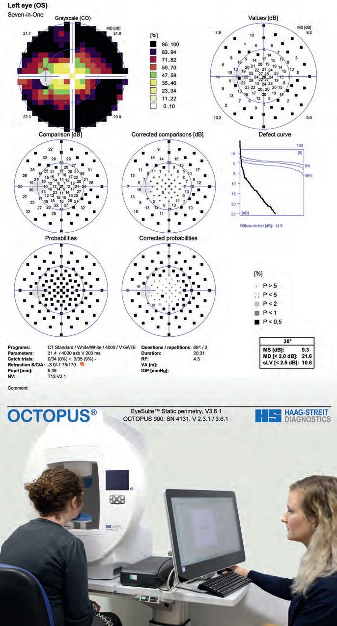
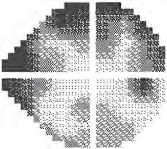
• Standard automated perimetry (SAP) is the method used routinely in most clinical situations. Automated perimeters in common use include the Humphrey Field Analyser (HFA), the Octopus, Medmont, Henson and Dicon (Figs 1.17 and 1.18). These predominantly utilize static testing, though software is available on some machines to perform dynamic assessment.
TIP Visual field results should always be used in conjunction with the clinical findings.
Testing algorithms
Threshold
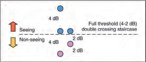
Threshold perimetry is used for detailed assessment of the hill of vision by plotting the threshold luminance value at various locations in the visual field and comparing the results with agematched ‘normal’ values. A typical automated strategy is to present a stimulus of higher than expected intensity. If seen, the intensity is decreased in steps (e.g. 4 dB) until it is no longer seen (‘staircasing’). The stimulus is then increased again (e.g. 2 dB steps) until seen once more (Fig. 1.19). If the stimulus is not seen initially, its intensity is increased in steps until seen. Essentially, the threshold is crossed in one direction with large increments, then crossed again to ‘fine-tune’ the result with smaller increments. Threshold testing is commonly used for monitoring glaucoma.
Suprathreshold
Suprathreshold perimetry involves testing with stimuli of luminance above the expected normal threshold levels for an agematched population to assess whether these are detected. In other words, testing to check that a subject can see stimuli that would be seen by a normal person of the same age. It enables testing to be carried out rapidly to indicate whether function is grossly normal or not and is usually reserved for screening.
Fast algorithms
In recent years strategies have been introduced with shorter testing times, providing efficiency benefits with little or no detriment to testing accuracy. The HFA offers the SITA (Swedish Interactive Thresholding Algorithm), which uses a database of normal and glaucomatous fields to estimate threshold values and takes responses during the test into account to arrive at adjusted estimates throughout the test. Full-threshold values are obtained at the start of the test for four points. SITA-Standard and SITAFast (Fig. 1.20) versions are available. The Octopus Perimeter
Fig. 1.17 Humphrey perimeter and printout
Fig. 1.18 Octopus perimeter and printout
uses G-TOP (Glaucoma Tendency Oriented Perimetry), which estimates thresholds based on information gathered from more detailed assessment of adjacent points. TOP presents each stimulus once at each location, instead of 4–6 times per location with a standard technique.
Testing patterns
• Glaucoma
○ Importance of central area. Most important defects in glaucoma occur centrally – within a 30° radius from the fixation point – so this is the area most commonly tested.
○ 24-2 is a routinely used glaucoma-orientated pattern. ‘24’ denotes the extent in degrees to which the field is tested on the temporal side (to 30° on the nasal side). The number after the hyphen (2) describes the pattern of the points tested. 30-2 is an alternative.
○ 10-2 is used to assess a central area of radius 10°. Glaucomatous defects here may threaten central vision. The 10-2 pattern facilitates more detailed monitoring of the extent of damage, especially in advanced glaucoma where there is ‘split’ fixation.
• Peripheral field. Patterns that include central and peripheral points (e.g. FF-120) are typically limited to the assessment of neurological defects.
• Binocular field testing (e.g. Esterman strategy) is used to assess statutory driving entitlement in many jurisdictions.
Analysis
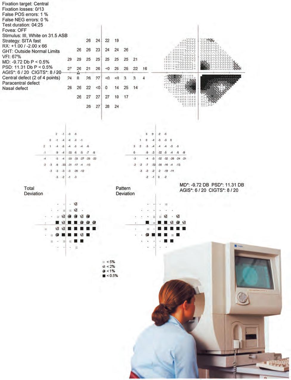
SAP provides the clinician with an array of clinically relevant information via monitor display or printout. The patient’s name and age are confirmed and a check made that any appropriate refractive error compensation was used. General information should be reviewed, such as the type of algorithm performed, the time taken for the test and the order in which the eyes were tested.
Reliability indices
Reliability indices (see Fig. 1.20, top left corner) reflect the extent to which the patient’s results are reliable. If significantly unreliable, further evaluation of the visual field printout is pointless. With SITA strategies, false negatives or false positives over about 15% should probably be regarded as significant and with full-threshold strategies, fixation losses over 20% and false positives or negatives
over 33%. In patients who consistently fail to achieve good reliability it may be useful to switch to a suprathreshold strategy or kinetic perimetry.
• Fixation losses indicate steadiness of gaze during the test. Methods of assessment include presentation of stimuli to the blind spot to ensure no response is recorded, and the use of a ‘gaze monitor’.
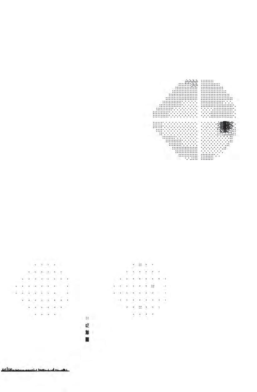
• False positives are usually assessed by decoupling a stimulus from its accompanying sound. If the sound alone is presented and the patient still responds, a false positive is recorded. With a high false-positive score the grey scale printout appears abnormally pale (Fig. 1.21). In SITA testing, false positives are estimated based on the response time.
• False negatives are registered by presenting a stimulus much brighter than threshold at a location where the threshold has already been determined. If the patient fails to respond, a false negative is recorded. A high false-negative score indicates inattention, tiredness or malingering, but is occasionally an indication of disease severity rather than unreliability. The grey scale printout in individuals with high false-negative responses tends to have a clover leaf shape (Fig. 1.22).
TIP If the reliability indices are poor, be careful when interpreting the results of a visual field test.
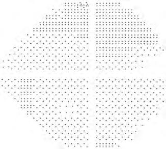
Sensitivity values
• A numerical display (see Fig. 1.20, upper left display) gives the measured or estimated (depending on strategy) threshold in dB at each point. In a full-threshold strategy, where the threshold is rechecked either as routine or because of an unexpected (>5 dB) result, the second result is shown in brackets next to the first.
• A grey scale represents the numerical display in graphical form (see Fig. 1.20, upper right display) and is the simplest display modality to interpret: decreasing sensitivity is represented by darker tones – the physiological blind spot is a darker area in the temporal field typically just below the horizontal axis. Each change in grey scale tone is equivalent to a 5 dB change in sensitivity at that location.
• Total deviation (see Fig. 1.20, middle left display) shows the difference between a test-derived threshold at a given point and the normal sensitivity at that point for the general population, correcting for age. Negative values indicate lower than normal sensitivity, positive values higher than normal.
• Pattern deviation (see Fig. 1.20, middle right display) is derived from total deviation values adjusted for any generalized decrease in sensitivity in the overall field (e.g. lens opacity), and demonstrates localized defects.
• Probability value plots of the total and pattern deviation (see Fig. 1.20, left and right lower displays) are a representation of the percentage (<5% to <0.5%) of the normal population in whom the measured defect at each point would be expected. Darker symbols represent a greater likelihood that a defect is significant.
Fig. 1.19 Determination of threshold
Single Field Analysis
Eye: Right Name:
Central 24-2 Threshold Test
Fixation Monitor: Gaze/Blind Spot
Fixation Target: Central
Fixation Losses: 0/10
False POS Errors: 0%
False NEG Errors: 0%
Test Duration: 02:42
Fover: OFF
Stimulus: III, White
Background: 31.5 ASB
Strategy: SITA-Fast 26 302930302929
– SITA-Fast printout (see text) (Copyright 2010 Carl Zeiss Meditec)
Date: 16-08-2013
Time: 2:12 PM Age: 68
Fig. 1.20 Humphrey perimeter
Single Field Analysis
Eye: Right Name: 1587884
Central 24-2 Threshold Test
Fixation Monitor: Gaze/Blind Spot
Fixation Target: Central Fixation Losses: 9/14
False POS Errors: 66%
False NEG Errors: 33%
Test Duration: 08:30
Fover: OFF
Stimulus: III, White
31.5 ASB
Pupil Diameter: Visual Acuity: RX: DS DC ×
Date: 14-02-2002
Time: 5:03 PM Age: 77
1.21
Single Field Analysis
Eye: Right Name:ID:DOB:
Central 24-2 Threshold Test
Fixation Monitor: Gaze/Blind Spot
Fixation Target: Central Fixation Losses: 0/17
False POS Errors: 3%
False NEG Errors: 53%
Test Duration: 08:52
Fover: OFF
Stimulus: III, White
Pupil Diameter: Visual Acuity: RX: +0.50 DS +1.00 DC × 30
DATE: Time: 3:33 PM Age: 85
Fig. 1.22 High false-negative score (arrow) with a clover leaf-shaped grey scale display