Preface to Fourth Edition
Introduction to Optimum Design, Fourth Edition presents an organized approach to optimizing the design of engineering systems. Basic concepts and procedures of optimization are illustrated with examples to show their applicability to engineering design problems. The crucial step of formulating a design optimization problem is detailed. The numerical process of refining an initial formulation of the optimization problem is illustrated and how to correct the initial formulation if it fails to produce a solution or does not produce an acceptable solution. This as well as other numerical aspects of the solution process for optimum design are consolidated in chapter: Optimum Design: Numerical Solution Process and Excel Solver. The pedagogical aspects of the material are addressed from student as well as teacher’s point of view. This is particularly true for the material of chapters: Introduction to Design Optimization, Optimum Design Problem Formulation, Graphical Solution Method and Basic Optimization Concepts, Optimum Design Concepts: Optimality Conditions, More on Optimum Design Concepts: Optimality Conditions, Optimum Design: Numerical Solution Process and Excel Solver, Optimum Design with MATLAB®, Linear Programming Methods for Optimum Design, More on Linear Programming Methods for Optimum Design, Numerical Methods for Unconstrained Optimum Design, More on Numerical Methods for Unconstrained Optimum Design, and Numerical Methods for Constrained Optimum Design that forms the
basis for a first course on optimum design. More detailed calculations are included in examples to illustrate procedures. Key ideas of various concepts are highlighted for easy reference.
Practical applications of optimization techniques are expanding rapidly, and to illustrate this, engineering design examples are presented throughout the text. Chapters: Optimum Design: Numerical Solution Process and Excel Solver, Optimum Design with MATLAB®, and Practical Applications of Optimization also address various aspects of practical applications of optimization with example problems. Many projects (identified with a *) based on practical applications are included as exercises at the end of chapters: Optimum Design Problem Formulation, Graphical Solution Method and Basic Optimization Concepts, Optimum Design: Numerical Solution Process and Excel Solver, Optimum Design with MATLAB®, Practical Applications of Optimization, Discrete Variable Optimum Design Concepts and Methods, and NatureInspired Search Methods.
Direct search methods that do not use any stochastic ideas in their search are presented in chapter: More on Numerical Methods for Unconstrained Optimum Design and those that do are presented in chapter: NatureInspired Search Methods. These methods do not require derivatives of the problem functions, therefore they are broadly applicable for practical applications and they are relatively easy to program and use.
The instructor’s manual that accompanies the text is comprehensive and user-friendly. The original problem statement for each exercise is included in the solution page for easy reference. Many MATLAB and Excel files for the problems are also included.
The text is broadly divided into three parts. Part I presents the basic concepts related to optimum design and optimality conditions in chapters: Introduction to Design Optimization 2 Optimum Design Problem Formulation, Graphical Solution Method and Basic Optimization Concepts, Optimum Design Concepts: Optimality Conditions, and More on Optimum Design Concepts: Optimality Conditions. Part II treats numerical methods for continuous variable smooth optimization problems and their practical applications in chapters: Optimum Design: Numerical Solution Process and Excel Solver, Optimum Design with MATLAB®, Linear Programming Methods for Optimum Design, More on Linear Programming Methods for Optimum Design, Numerical Methods for Unconstrained Optimum Design, More on Numerical Methods for Unconstrained Optimum Design, Numerical Methods for Constrained Optimum Design, More on Numerical Methods for Constrained Optimum Design, Practical Applications of Optimization. Part III contains advanced topics of practical interest on optimum design, including nature-inspired metaheuristic methods that do not require derivatives of the problem functions in chapters: Discrete Variable Optimum Design Concepts and Methods, Global Optimization Concepts and Methods, Nature-Inspired Search Methods, Multi-objective Optimum Design Concepts and Methods, and Additional Topics on Optimum Design. Introduction to Optimum Design, Fourth Edition can be used to design several types of courses depending on the learning objectives
for students. Three courses are suggested, although several variations are possible.
Undergraduate/First-Year Graduate Level Course
Topics for an undergraduate and/or firstyear graduate course include:
• Formulation of optimization problems (see chapters: Introduction to Design Optimization and Optimum Design Problem Formulation)
• Optimization concepts using the graphical method (see chapter: Graphical Solution Method and Basic Optimization Concepts)
• Optimality conditions for unconstrained and constrained problems (see chapter: Optimum Design Concepts: Optimality Conditions)
• Use of Excel and MATLAB® illustrating optimum design of practical problems (see chapters: Optimum Design: Numerical Solution Process and Excel Solver and Optimum Design with MATLAB®)
• Linear programming (see chapter: Linear Programming Methods for Optimum Design)
• Numerical methods for unconstrained and constrained problems (see chapters: Numerical Methods for Unconstrained Optimum Design and Numerical Methods for Constrained Optimum Design)
The use of Excel and MATLAB should be introduced mid-semester so that students have a chance to formulate and solve more challenging projects by the semester’s end. Note that project exercises and sections with advanced material are marked with an asterisk (*) next to section headings, which means that they may be omitted for this course.
First Graduate-Level Course
Topics for a first graduate-level course include
• Theory and numerical methods for unconstrained optimization (see chapters: Introduction to Design Optimization, Optimum Design Problem Formulation, Graphical Solution Method and Basic Optimization Concepts, Optimum Design Concepts: Optimality Conditions, Numerical Methods for Unconstrained Optimum Design, and More on Numerical Methods for Unconstrained Optimum Design)
• Theory and numerical methods for constrained optimization (see chapters: Optimum Design Concepts: Optimality Conditions, More on Optimum Design Concepts: Optimality Conditions, Numerical Methods for Constrained Optimum Design, and More on Numerical Methods for Constrained Optimum Design)
• Linear and quadratic programming (see chapters: Linear Programming Methods for Optimum Design and More on Linear Programming Methods for Optimum Design)
The pace of material can be a bit faster for this course. Students should code some of the algorithms into computer programs and solve some projects based on practical applications.
Second Graduate-Level Course
This course presents advanced topics on optimum design:
• Duality theory in nonlinear programming, rate of convergence
of iterative algorithms, derivation of numerical methods, and direct search methods (see chapters: Introduction to Design Optimization, Optimum Design Problem Formulation, Graphical Solution Method and Basic Optimization Concepts, Optimum Design Concepts: Optimality Conditions, More on Optimum Design Concepts: Optimality Conditions, Optimum Design: Numerical Solution Process and Excel Solver, Optimum Design with MATLAB®, Linear Programming Methods for Optimum Design, More on Linear Programming Methods for Optimum Design, Numerical Methods for Unconstrained Optimum Design, More on Numerical Methods for Unconstrained Optimum Design, and Numerical Methods for Constrained Optimum Design, More on Numerical Methods for Constrained Optimum Design, and Practical Applications of Optimization)
• Methods for discrete variable problems (see chapter: Discrete Variable Optimum Design Concepts and Methods)
• Global optimization (see chapter: Global Optimization Concepts and Methods)
• Nature-inspired search methods (see chapter: Nature-Inspired Search Methods)
• Multi-objective optimization (see chapter: Multi-objective Optimum Design Concepts and Methods)
• Response surface methods, robust design, and reliability-based design optimization (see chapter: Additional Topics on Optimum Design)
In this course, students write computer programs to implement some of the numerical methods to gain experience with their coding and to solve practical problems.
1 Introduction to Design Optimization
Upon completion of this chapter, you will be able to:
• Describe the overall process of designing systems
• Distinguish between engineering design and engineering analysis activities
• Distinguish between the conventional design process and optimum design process
• Distinguish between optimum design and optimal control problems
• Understand the notations used for operations with vectors, matrices, and functions and their derivatives
Engineering consists of a number of well-established activities, including analysis, design, fabrication, sales, research, and development of systems. The subject of this text—the design of systems—is a major field in the engineering profession. The process of designing and fabricating systems has been developed over centuries. The existence of many complex systems, such as buildings, bridges, highways, automobiles, airplanes, space vehicles, and others, is an excellent testimonial to its long history. However, the evolution of such systems has been slow and the entire process is both time-consuming and costly, requiring substantial human and material resources. Therefore, the procedure is to design, fabricate, and use a system regardless of whether it is the best one. Improved systems have been designed only after a substantial investment has been recovered.
The preceding discussion indicates that several systems can usually accomplish the same task, and that some systems are better than others. For example, the purpose of a bridge is to provide continuity in traffic from one side of the river to the other. Several types of bridges can serve this purpose. However, to analyze and design all possibilities can be timeconsuming and costly. Usually one type is selected based on some preliminary analyses and is designed in detail.
The design of a system can be formulated as a problem of optimization in which a performance measure is optimized while all other requirements are satisfied. Many numerical methods of optimization have been developed and used to design better systems. This text describes the basic concepts of optimization and numerical methods for the design of engineering systems. Design process, rather than optimization theory, is emphasized. Various theorems are stated
Introduction to Optimum Design. http://dx.doi.org/10.1016/B978-0-12-800806-5.00001-9
Copyright © 2017 Elsevier Inc. All rights reserved.
as results without rigorous proofs. However, their implications from an engineering point of view are discussed.
any problem in which certain parameters need to be determined to satisfy constraints can be formulated as an optimization problem. once this has been done, optimization concepts and methods described in this text can be used to solve it. optimization methods are quite general, having a wide range of applicability in diverse fields. It is not possible to discuss every application of optimization concepts and methods in this introductory text. However, using simple applications, we discuss concepts, fundamental principles, and basic techniques that are used in most applications. The student should understand them without getting bogged down with notations, terminologies, and details on particular areas of application.
1.1 THE DESIGN PROCESS
How Do I Begin to Design a System?
Designing engineering systems can be a complex process. assumptions must be made to develop realistic models that can be subjected to mathematical analysis by the available methods. The models may need to be verified by experiments. Many possibilities and factors must be considered during the optimization problem formulation phase. Economic considerations play an important role in designing cost-effective systems. To complete the design of an engineering system, designers from different fields of engineering must usually cooperate. For example, the design of a high-rise building involves designers from architectural, structural, mechanical, electrical, and environmental engineering, as well as construction management experts. Design of a passenger car requires cooperation among structural, mechanical, automotive, electrical, chemical, hydraulics design, and human factor engineers. Thus, in an interdisciplinary environment, considerable interaction is needed among design teams to complete the project. For most applications, the entire design project must be broken down into several subproblems, which are then treated somewhat independently. Each of the subproblems can be posed as a problem of optimum design.
The design of a system begins with the analysis of various options. Subsystems and their components are identified, designed, and tested. This process results in a set of drawings, calculations, and reports with the help of which the system can be fabricated. We use a systems engineering model to describe the design process. although complete discussion of this subject is beyond the scope of this text, some basic concepts are discussed using a simple block diagram.
Design is an iterative process. Iterative implies analyzing several trial designs one after another until an acceptable design is obtained. It is important to understand the concept of a trial design. In the design process, the designer estimates a trial design of the system based on experience, intuition, or some simple mathematical analyses. The trial design is then analyzed to determine if it is acceptable. In case it gets accepted, the design process is terminated. In the optimization process, the trial design is analyzed to determine if it is the best. Depending on the specifications, “best” can have different connotations for different systems. In general, it implies that a system is cost-effective, efficient, reliable, and durable.
The basic concepts are described in this text to aid the engineer in designing systems at minimum cost.
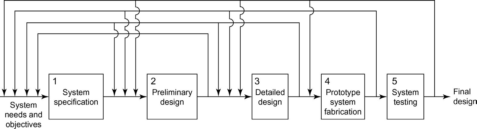
The design process should be well organized. To discuss it, we consider a system evolution model, shown in Fig. 1.1, where the process begins with the identification of a need that may be conceived by engineers or nonengineers. The five steps of the model in the figure are described in the following paragraphs.
1. The first step in the evolutionary process is to precisely define the specifications for the system. considerable interaction between the engineer and the sponsor of the project is usually necessary to quantify the system specifications.
2. The second step in the process is to develop a preliminary design of the system. Various system concepts are studied. Since this must be done in a relatively short time, simplified models are used at this stage. Various subsystems are identified and their preliminary designs are estimated. Decisions made at this stage generally influence the system’s final appearance and performance. at the end of the preliminary design phase, a few promising design concepts that need further analysis are identified.
3. The third step in the process is a detailed design for all subsystems using the iterative process described earlier. To evaluate various possibilities, this must be done for all previously identified promising design concepts. The design parameters for the subsystems must be identified. The system performance requirements must be identified and formulated. The subsystems must be designed to maximize system worth or to minimize a measure of the cost. Systematic optimization methods described in this text aid the designer in accelerating the detailed design process. at the end of the process, a description of the final design is available in the form of reports and drawings.
4. The fourth and fifth steps shown in Fig. 1.1 may or may not be necessary for all systems. They involve fabrication of a prototype system and testing, and are necessary when the system must be mass-produced or when human lives are involved. These steps may appear to be the final ones in the design process, but they are not because the system may not perform according to specifications during the testing phase. Therefore, the specifications may have to be modified or other concepts may have to be studied. In fact, this reexamination may be necessary at any point during the design process. It is for this reason that feedback loops are placed at every stage of the system evolution process, as shown in Fig. 1.1. This iterative process must be continued until the best system evolves.
FIGURE 1.1 System evolution model.
Depending on the complexity of the system, this process may take a few days or several months.
The model described in Fig. 1.1 is a simplified block diagram for system evolution. In actual practice, each block may be broken down into several subblocks to carry out the studies properly and arrive at rational decisions. The important point is that optimization concepts and methods are helpful at every stage of the process. Such methods, along with the appropriate software, can be useful in studying various design possibilities rapidly.
1.2 ENGINEERING DESIGN VERSUS ENGINEERING ANALYSIS
Can I Design Without Analysis?
No, You Must Analyze!
It is important to recognize the differences between engineering analysis and design activities The analysis problem is concerned with determining the behavior of an existing system or a trial system being designed for a known task. Determination of the behavior of the system implies calculation of its response to specified inputs. For this reason, the sizes of various parts and their configurations are given for the analysis problem; that is, the design of the system is known. on the other hand, the design process calculates the sizes and shapes of various parts of the system to meet performance requirements.
The design of a system is an iterative process. We estimate a trial design and analyze it to see if it performs according to given specifications. If it does, we have an acceptable (feasible) design, although we may still want to change it to improve its performance. If the trial design does not work, we need to change it to come up with an acceptable system. In both cases, we must be able to analyze designs to make further decisions. Thus, analysis capability must be available in the design process.
This book is intended for use in all branches of engineering. It is assumed throughout that students understand the analysis methods covered in undergraduate engineering statics and physics courses. However, we will not let the lack of analysis capability hinder understanding of the systematic process of optimum design. Equations for analysis of the system are given wherever feasible.
1.3 CONVENTIONAL VERSUS OPTIMUM DESIGN PROCESS
Why Do I Want to Optimize?
Because You Want to Beat the Competition and Improve Your Bottom Line!
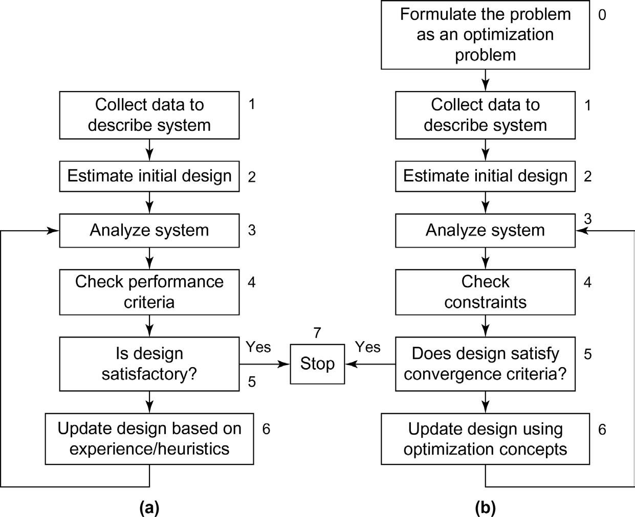
It is a challenge for engineers to design efficient and cost-effective systems without compromising their integrity. Fig. 1.2a presents a self-explanatory flowchart for a conventional design method; Fig. 1.2b presents a similar flowchart for the optimum design method. It is important to note that both methods are iterative, as indicated by a loop between blocks 6 and 3. Both methods have some blocks that require similar calculations and others that require different calculations. The key features of the two processes are as follows.
0. The optimum design method has block 0, where the problem is formulated as one of optimization (see chapter: optimum Design problem Formulation for detailed discussion). an objective function is defined that measures the merits of different designs.
1. Both methods require data to describe the system in block 1.
2. Both methods require an initial design estimate in block 2.
3. Both methods require analysis of the system in block 3.
4. In block 4, the conventional design method checks to ensure that the performance criteria are met, whereas the optimum design method checks for satisfaction of all of the constraints for the problem formulated in block 0.
5. In block 5, stopping criteria for the two methods are checked, and the iteration is stopped if the specified stopping criteria are met.
6. In block 6, the conventional design method updates the design based on the designer’s experience and intuition and other information gathered from one or more trial designs; the optimum design method uses optimization concepts and procedures to update the current design.
The foregoing distinction between the two design approaches indicates that the conventional design process is less formal. an objective function that measures a design’s merit is not identified. Trend information is usually not calculated; nor is it used in block 6 to make design decisions for system improvement. In contrast, the optimization process is more formal, using trend information to make design changes.
FIGURE 1.2 comparison of: (a) conventional design method; and (b) optimum design method.
1.4 OPTIMUM DESIGN VERSUS OPTIMAL CONTROL
What Is Optimal Control?
optimum design and optimal control of systems are separate activities. There are numerous applications in which methods of optimum design are useful in designing systems. There are many other applications where optimal control concepts are needed. In addition, there are some applications in which both optimum design and optimal control concepts must be used. Sample applications of both techniques include robotics and aerospace structures. In this text, optimal control problems and methods are not described in detail. However, the fundamental differences between the two activities are briefly explained in the sequel. It turns out that some optimal control problems can be transformed into optimum design problems and treated by the methods described in this text. Thus, methods of optimum design are very powerful and should be clearly understood. a simple optimal control problem is described in chapter: practical applications of optimization and is solved by the methods of optimum design.
The optimal control problem consists of finding feedback controllers for a system to produce the desired output. The system has active elements that sense output fluctuations. System controls are automatically adjusted to correct the situation and optimize a measure of performance. Thus, control problems are usually dynamic in nature. In optimum design, on the other hand, we design the system and its elements to optimize an objective function. The system then remains fixed for its entire life.
as an example, consider the cruise control mechanism in passenger cars. The idea behind this feedback system is to control fuel injection to maintain a constant speed. Thus, the system’s output (ie, the vehicle’s cruising speed) is known. The job of the control mechanism is to sense fluctuations in speed depending on road conditions and to adjust fuel injection accordingly.
1.5 BASIC TERMINOLOGY AND NOTATION
Which Notation Do I Need to Know?
To understand and to be comfortable with the methods of optimum design, a student must be familiar with linear algebra (vector and matrix operations) and basic calculus. operations of linear algebra are described in appendix a. Students who are not comfortable with this material need to review it thoroughly. calculus of functions of single and multiple variables must also be understood. calculus concepts are reviewed wherever they are needed. In this section, the standard terminology and notations used throughout the text are defined. It is important to understand and memorize these notations and operations.
1.5.1 Vectors and Points
Since realistic systems generally involve several variables, it is necessary to define and use some convenient and compact notations to represent them. Set and vector notations serve this purpose quite well.
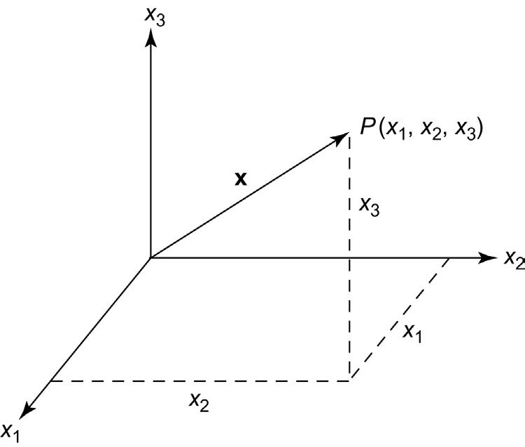
1.3 Vector representation of a point P in 3D space.
A point is an ordered list of numbers Thus, (x1, x2) is a point consisting of two numbers whereas (x1, x2, …, xn) is a point consisting of n numbers. Such a point is often called an n-tuple. The n components x1, x2, …, xn are collected into a column vector as
where the superscript T denotes the transpose of a vector or a matrix. This is called an n-vector. Each number xi is called a component of the (point) vector. Thus, x1 is the first component, x2 is the second, and so on.
We also use the following notation to represent a point or a vector in the n-dimensional space:
In 3-dimensional (3D) space, the vector x = [x1 x2 x3]T represents a point P, as shown in Fig. 1.3. Similarly, when there are n components in a vector, as in Eqs. (1.1) and (1.2), x is interpreted as a point in the n-dimensional space, denoted as Rn. The space Rn is simply the collection of all n-dimensional vectors (points) of real numbers. For example, the real line is R1, the plane is R2 , and so on.
The terms vector and point are used interchangeably, and lowercase letters in roman boldface are used to denote them. Uppercase letters in roman boldface represent matrices.
1.5.2 Sets
often we deal with sets of points satisfying certain conditions. For example, we may consider a set S of all points having three components, with the last having a fixed value of 3, which is written as
FIGURE
() == = Sx xx x x ,, 3 12 33 (1.3)
Information about the set is contained in braces ({ }). Eq. (1.3) reads as “S equals the set of all points (x1, x2, x3) with x3 = 3.” The vertical bar divides information about the set S into two parts: To the left of the bar is the dimension of points in the set; to the right are the properties that distinguish those points from others not in the set (eg, properties a point must possess to be in the set S).
Members of a set are sometimes called elements. If a point x is an element of the set S, then we write x ∈ S. The expression x ∈ S is read as “ x is an element of (belongs to) S.” conversely, the expression “ y ∉ S” is read as “ y is not an element of (does not belong to) S.”
If all the elements of a set S are also elements of another set T, then S is said to be a subset of T. Symbolically, we write S ⊂ T, which is read as “S is a subset of T” or “S is contained in T.” alternatively, we say “T is a superset of S,” which is written as T ⊃ S.
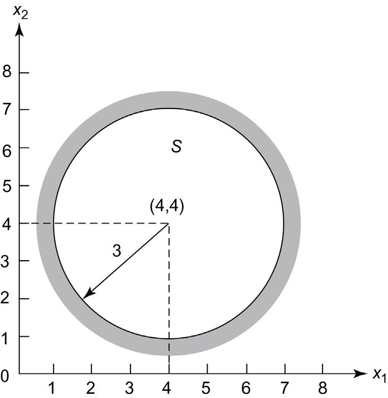
as an example of a set S, consider a domain of the xl – x2 plane enclosed by a circle of radius 3 with the center at the point (4, 4), as shown in Fig. 1.4 Mathematically, all points within and on the circle can be expressed as
Thus, the center of the circle (4, 4) is in the set S because it satisfies the inequality in Eq. (1.4) We write this as (4, 4) ∈ S The origin of coordinates (0, 0) does not belong to the set because it does not satisfy the inequality in Eq. (1.4) We write this as (0, 0) ∉ S. It can be verified that the following points belong to the set: (3, 3), (2, 2), (3, 2), (6, 6). In fact, set S has an infinite number of points. Many other points are not in the set. It can be verified that the following points are not in the set: (1, 1), (8, 8), and ( 1, 2).
FIGURE 1.4 Geometrical representation of
1.5.3 Notation for Constraints
constraints arise naturally in optimum design problems. For example, the material of the system must not fail, the demand must be met, resources must not be exceeded, and so on. We shall discuss the constraints in more detail in chapter: optimum Design problem Formulation. Here we discuss the terminology and notations for the constraints.
We encountered a constraint in Fig. 1.4 that shows a set S of points within and on the circle of radius 3. The set S is defined by the following constraint:
a constraint of this form is a “less than or equal to type” constraint and is abbreviated as “≤ type.” Similarly, there are greater than or equal to type constraints, abbreviated as “≥ type.” Both are called inequality constraints.
1.5.4 Superscripts/Subscripts and Summation Notation
Later we will discuss a set of vectors, components of vectors, and multiplication of matrices and vectors. To write such quantities in a convenient form, consistent and compact notations must be used. We define these notations here. Superscripts are used to represent different vectors and matrices. For example, x(i) represents the ith vector of a set and A(k) represents the kth matrix. Subscripts are used to represent components of vectors and matrices. For example, xj is the jth component of x and aij is the i–jth element of matrix A. Double subscripts are used to denote elements of a matrix.
To indicate the range of a subscript or superscript we use the notation
This represents the numbers x1, x2, …, xn. note that “i = 1 to n” represents the range for the index i and is read, “i goes from 1 to n.” Similarly, a set of k vectors, each having n components, is represented by the superscript notation as jk x ;1 to j = ()
This represents the k vectors x(l) , x(2) , …, x(k) . It is important to note that subscript i in Eq. (1.6) and superscript j in Eq. (1.7) are free indices; that is, they can be replaced by any other variable. For example, Eq. (1.6) can also be written as xj, j = 1 to n and Eq. (1.7) can be written as x(i) , i = 1 to k. note that the superscript j in Eq. (1.7) does not represent the power of x. It is an index that represents the jth vector of a set of vectors. We also use the summation notation quite frequently. For example, cx yx yx y ... nn 11 22 =+ ++ (1.8) is written as
also, multiplication of an n-dimensional vector x by an m × n matrix A to obtain an mdimensional vector y is written as
(1.10) or, in summation notation, the ith component of y is
There is another way of writing the matrix multiplication of Eq. (1.10). Let m-dimensional vectors a(i); i = 1 to n represent columns of the matrix A. Then y = Ax is also written as
The sum on the right side of Eq. (1.12) is said to be a linear combination of columns of matrix A with xj, j = 1 to n as its multipliers. or y is given as a linear combination of columns of A (refer appendix a for further discussion of the linear combination of vectors). occasionally, we must use the double summation notation. For example, assuming m = n and substituting yi from Eq. (1.11) into Eq. (1.9), we obtain the double sum as
note that the indices i and j in Eq. (1.13) can be interchanged. This is possible because c is a scalar quantity, so its value is not affected by whether we sum first on i or on j. Eq. (1.13) can also be written in the matrix form, as we will see later.
1.5.5 Norm/Length of a Vector
If we let x and y be two n-dimensional vectors, then their dot product is defined as
Thus, the dot product is a sum of the product of corresponding elements of the vectors x and y. Two vectors are said to be orthogonal (normal) if their dot product is 0; that is, x and y are orthogonal if (x • y) = 0. If the vectors are not orthogonal, the angle between them can be calculated from the definition of the dot product:
xy xy cos, (1.15)
where u is the angle between vectors x and y, and ‖x‖ represents the length of vector x (also called the norm of the vector). The length of vector x is defined as the square root of the sum of squares of the components:
The double sum of Eq. (1.13) can be written in the matrix form as follows:
Since Ax represents a vector, the triple product of Eq. (1.17) is also written as a dot product:
1.5.6 Functions of Several Variables
Just as a function of a single variable is represented as f(x), a function of n independent variables x1, x2, …, xn is written as
We deal with many functions of vector variables. To distinguish between functions, subscripts are used. Thus, the ith function is written as
If there are m functions gi(x), i = 1 to m, these are represented in the vector form
Throughout the text it is assumed that all functions are continuous and at least twice continuously differentiable. a function f(x) of n variables is continuous at a point x* if, for any ε > 0, there is a d > 0 such that
whenever ‖x x*‖ < d. Thus, for all points x in a small neighborhood of point x*, a change in the function value from x* to x is small when the function is continuous. a continuous function need not be differentiable. Twice-continuous differentiability of a function implies not only that it is differentiable two times, but also that its second derivative is continuous.
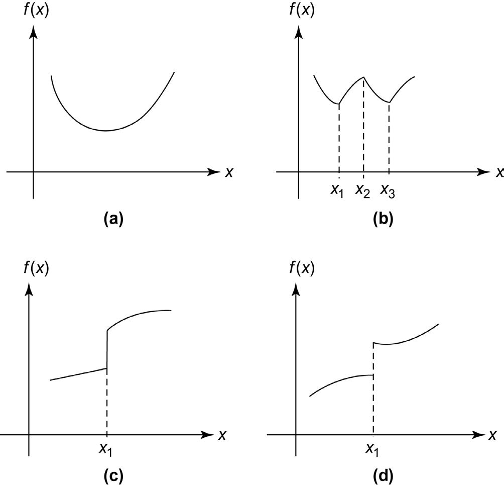
Fig. 1.5a,b shows continuous and discontinuous functions. The function in Fig. 1.5a is differentiable everywhere, whereas the function in Fig. 1.5b is not differentiable at points x1, x2, and x3. Fig. 1.5c is an example in which f is not a function because it has infinite values at x1. Fig. 1.5d is an example of a discontinuous function. as examples, functions f(x) = x3
FIGURE 1.5 Continuous and discontinuous functions. (a) and (b) continuous functions; (c) not a function; and (d) discontinuous function.
and f(x) = sinx are continuous everywhere and are also continuously differentiable. However, function f(x) = |x| is continuous everywhere but not differentiable at x = 0.
1.5.7 Partial Derivatives of Functions
often in this text we must calculate derivatives of functions of several variables. Here we introduce some of the basic notations used to represent the partial derivatives of functions of several variables.
First Partial Derivatives
For a function f(x) of n variables, the first partial derivatives are written as
The n partial derivatives in Eq. (1.23) are usually arranged in a column vector known as the gradient of the function f(x). The gradient is written as ∂f/∂x or ∇f(x). Therefore,
note that each component of the gradient in Eqs. (1.23) or (1.24) is a function of vector x.
Second Partial Derivatives
Each component of the gradient vector in Eq. (1.24) can be differentiated again with respect to a variable to obtain the second partial derivatives for the function f(x):
We see that there are n2 partial derivatives in Eq. (1.25). These can be arranged in a matrix known as the Hessian matrix, written as H(x), or simply the matrix of second partial derivatives of f(x), written as ∇2f(x):
note that if f(x) is continuously differentiable two times, then Hessian matrix H(x) in Eq. (1.26) is symmetric
Partial Derivatives of Vector Functions
on several occasions we must differentiate a vector function of n variables, such as the vector g(x) in Eq. (1.21), with respect to the n variables in vector x. Differentiation of each component of the vector g(x) results in a gradient vector, such as ∇gi(x). Each of these gradients is an n-dimensional vector. They can be arranged as columns of a matrix of dimension n × m, referred to as the gradient matrix of g(x). This is written as
This gradient matrix is usually written as matrix A:
1.5.8 US–British Versus SI Units
The formulation of the design problem and the methods of optimization do not depend on the units of measure used. Thus, it does not matter which units are used to formulate the problem. However, the final form of some of the analytical expressions for the problem does depend on the units used. In the text, we use both US–British and SI units in examples and exercises. Readers unfamiliar with either system should not feel at a disadvantage when reading and understanding the material since it is simple to switch from one system to the other. To facilitate the conversion from US–British to SI units or vice versa, Table 1.1 gives
TABLE 1.1
Conversion Factors for uS–British and SI units
To convert from US–British To SI units Multiply by Acceleration
Foot/second2 (ft./s2)
Inch/second2 (in./s2)
Area
Foot2 (ft.2)
Inch2 (in.2)
Bending moment or torque
Meter/second2 (m/s2) 0.3048*
Meter/second2 (m/s2) 0.0254*
Meter2 (m2) 0.09290304*
Meter2 (m2) 6.4516E–04*
pound force inch (lbf·in.) newton meter (n·m) 0.1129848
pound force foot (lbf·ft.) newton meter (n·m) 1.355818
Density
pound mass/inch3 (lbm/in.3)
pound mass/foot3 (lbm/ft.3)
Energy or work
Kilogram/meter3 (kg/m3) 27,679.90
Kilogram/meter3 (kg/m3) 16.01846
British thermal unit (BTU) Joule (J) 1055.056
Foot pound force (ft.·lbf) Joule (J) 1.355818
Kilowatt-hour (KWh) Joule (J) 3,600,000*
Force
Kip (1000 lbf) newton (n) 4448.222
pound force (lbf) newton (n) 4.448222
Length
Foot (ft.)
Inch (in.)
Inch (in.)
Meter (m) 0.3048*
Meter (m) 0.0254*
Micron (m); micrometer (mm) 25,400*
Mile (mi), US statute Meter (m) 1609.344
Mile (mi), International, nautical Meter (m) 1852*
Mass
pound mass (lbm) Kilogram (kg) 0.4535924 ounce Grams 28.3495
Slug (lbf·s2ft.)
Ton (short, 2000 lbm)
Ton (long, 2240 lbm)
Tonne (t, metric ton)
Power
Kilogram (kg) 14.5939
Kilogram (kg) 907.1847
Kilogram (kg) 1016.047
Kilogram (kg) 1000*
Foot pound/minute (ft.·lbf/min) Watt (W) 0.02259697
Horsepower (550 ft. lbf/s) Watt (W) 745.6999
TABLE 1.1 Conversion Factors for uS–British and SI units (cont.)
To convert from US–British To SI units
Multiply by Pressure or stress
atmosphere (std) (14.7 lbf/in.2)
newton/meter2 (n/m2 or pa) 101,325* one bar (b)
pound/foot2 (lbf/ft.2)
pound/inch2 (lbf/in.2 or psi)
Velocity
Foot/minute (ft./min)
Foot/second (ft./s)
newton/meter2 (n/m2 or pa) 100,000*
newton/meter2 (n/m2 or pa) 47.88026
newton/meter2 (n/m2 or pa) 6894.757
Meter/second (m/s) 0.00508*
Meter/second (m/s) 0.3048*
Knot (nautical mi/h), international Meter/second (m/s) 0.5144444
Mile/hour (mi/h), international Meter/second (m/s) 0.44704*
Mile/hour (mi/h), international Kilometer/hour (km/h) 1.609344*
Mile/second (mi/s), international Kilometer/second (km/s) 1.609344*
Volume
Foot3 (ft.3)
Inch3 (in.3)
Gallon (canadian liquid)
Gallon (UK liquid)
Gallon (UK liquid)
Gallon (US dry)
Gallon (US liquid)
Gallon (US liquid)
one liter (L)
one liter (L)
one milliliter (mL)
ounce (UK fluid)
ounce (US fluid)
ounce (US fluid)
ounce (US fluid)
pint (US dry)
pint (US liquid)
pint (US liquid)
Quart (US dry)
Quart (US liquid)
* Exact conversion factor.
Meter3 (m3) 0.02831685
Meter3 (m3) 1.638706E–05
Meter3 (m3) 0.004546090
Meter3 (m3) 0.004546092
Liter (L) 4.546092
Meter3 (m3) 0.004404884
Meter3 (m3) 0.003785412
Liter (L) 3.785412
Meter3 (m3) 0.001*
centimeter3 (cm3) 1000*
centimeter3 (cm3) 1*
Meter3 (m3)
2.841307E–05
Meter3 (m3) 2.957353E–05
Liter (L) 2.957353E–02
Milliliter (mL) 29.57353
Meter3 (m3) 5.506105E–04
Liter (L) 4.731765E–01
Meter3 (m3) 4.731765E–04
Meter3 (m3) 0.001101221
Meter3 (m3) 9.463529E–04
conversion factors for the most commonly used quantities. For a complete list of conversion factors, consult the IEEE/aSTM (2010) publication.
Reference
IEEE/aSTM, 2010. american national Standard for Metric practice. SI 10-2010. The Institute of Electrical and Electronics Engineers/american Society for Testing of Materials, new York.
I. THE BaSIc concEpTS