Imaging Life
Image Acquisition
and Analysis in Biology and Medicine
Lawrence R. Griffing
Biology Department
Texas A&M University Texas, United States
Contents
Preface xii
Acknowledgments xiv
About the Companion Website xv
Section 1 Image Acquisition 1
1 Image Structure and Pixels 3
1.1 The Pixel Is the Smallest Discrete Unit of a Picture 3
1.2 The Resolving Power of a Camera or Display Is the Spatial Frequency of Its Pixels 6
1.3 Image Legibility Is the Ability to Recognize Text in an Image by Eye 7
1.4 Magnification Reduces Spatial Frequencies While Making Bigger Images 9
1.5 Technology Determines Scale and Resolution 11
1.6 The Nyquist Criterion: Capture at Twice the Spatial Frequency of the Smallest Object Imaged 12
1.7 Archival Time, Storage Limits, and the Resolution of the Display Medium Influence Capture and Scan Resolving Power 13
1.8 Digital Image Resizing or Scaling Match the Captured Image Resolution to the Output Resolution 14
1.9 Metadata Describes Image Content, Structure, and Conditions of Acquisition 16
2 Pixel Values and Image Contrast 20
2.1 Contrast Compares the Intensity of a Pixel with That of Its Surround 20
2.2 Pixel Values Determine Brightness and Color 21
2.3 The Histogram Is a Plot of the Number of Pixels in an Image at Each Level of Intensity 24
2.4 Tonal Range Is How Much of the Pixel Depth Is Used in an Image 25
2.5 The Image Histogram Shows Overexposure and Underexposure 26
2.6 High-Key Images Are Very Light, and Low-Key Images Are Very Dark 27
2.7 Color Images Have Various Pixel Depths 27
2.8 Contrast Analysis and Adjustment Using Histograms Are Available in Proprietary and Open-Source Software 29
2.9 The Intensity Transfer Graph Shows Adjustments of Contrast and Brightness Using Input and Output Histograms 30
2.10 Histogram Stretching Can Improve the Contrast and Tonal Range of the Image without Losing Information 32
2.11 Histogram Stretching of Color Channels Improves Color Balance 32
2.12 Software Tools for Contrast Manipulation Provide Linear, Non-linear, and Output-Visualized Adjustment 34
2.13 Different Image Formats Support Different Image Modes 36
2.14 Lossless Compression Preserves Pixel Values, and Lossy Compression Changes Them 37
3 Representation and Evaluation of Image Data 42
3.1 Image Representation Incorporates Multiple Visual Elements to Tell a Story 42
3.2 Illustrated Confections Combine the Accuracy of a Typical Specimen with a Science Story 42
3.3 Digital Confections Combine the Accuracy of Photography with a Science Story 45
3.4 The Video Storyboard Is an Explicit Visual Confection 48
3.5 Artificial Intelligence Can Generate Photorealistic Images from Text Stories 48
3.6 Making Images Believable: Show Representative Images and State the Acquisition Method 50
3.7 Making Images Understood: Clearly Identify Regions of Interest with Suitable Framing, Labels, and Image Contrast 51
3.8 Avoid Dequantification and Technical Artifacts While Not Hesitating to Take the Picture 55
3.9 Accurate, Reproducible Imaging Requires a Set of Rules and Guidelines 56
3.10 The Structural Similarity Index Measure Quantifies Image Degradation 57
4 Image Capture by Eye 61
4.1 The Anatomy of the Eye Limits Its Spatial Resolution 61
4.2 The Dynamic Range of the Eye Exceeds 11 Orders of Magnitude of Light Intensity, and Intrascene Dynamic Range Is about 3 Orders 63
4.3 The Absorption Characteristics of Photopigments of the Eye Determines Its Wavelength Sensitivity 63
4.4 Refraction and Reflection Determine the Optical Properties of Materials 67
4.5 Movement of Light Through the Eye Depends on the Refractive Index and Thickness of the Lens, the Vitreous Humor, and Other Components 69
4.6 Neural Feedback in the Brain Dictates Temporal Resolution of the Eye 69
4.7 We Sense Size and Distribution in Large Spaces Using the Rules of Perspective 70
4.8 Three-Dimensional Representation Depends on Eye Focus from Different Angles 71
4.9 Binocular Vision Relaxes the Eye and Provides a Three-Dimensional View in Stereomicroscopes 74
5 Image Capture with Digital Cameras 78
5.1 Digital Cameras are Everywhere 78
5.2 Light Interacts with Silicon Chips to Produce Electrons 78
5.3 The Anatomy of the Camera Chip Limits Its Spatial Resolution 80
5.4 Camera Chips Convert Spatial Frequencies to Temporal Frequencies with a Series of Horizontal and Vertical Clocks 82
5.5 Different Charge-Coupled Device Architectures Have Different Read-out Mechanisms 85
5.6 The Digital Camera Image Starts Out as an Analog Signal that Becomes Digital 87
5.7 Video Broadcast Uses Legacy Frequency Standards 88
5.8 Codecs Code and Decode Digital Video 89
5.9 Digital Video Playback Formats Vary Widely, Reflecting Different Means of Transmission and Display 91
5.10 The Light Absorption Characteristics of the Metal Oxide Semiconductor, Its Filters, and Its Coatings Determine the Wavelength Sensitivity of the Camera Chip 91
5.11 Camera Noise and Potential Well Size Determine the Sensitivity of the Camera to Detectable Light 93
5.12 Scientific Camera Chips Increase Light Sensitivity and Amplify the Signal 97
5.13 Cameras for Electron Microscopy Use Regular Imaging Chips after Converting Electrons to Photons or Detect the Electron Signal Directly with Modified CMOS 99
5.14 Camera Lenses Place Additional Constraints on Spatial Resolution 101
5.15 Lens Aperture Controls Resolution, the Amount of Light, the Contrast, and the Depth of Field in a Digital Camera 106
5.16 Relative Magnification with a Photographic Lens Depends on Chip Size and Lens Focal Length 107
6 Image Capture by Scanning Systems 111
6.1 Scanners Build Images Point by Point, Line by Line, and Slice by Slice 111
6.2 Consumer-Grade Flatbed Scanners Provide Calibrated Color and Relatively High Resolution Over a Wide Field of View 111
6.3
Scientific-Grade Flatbed Scanners Can Detect Chemiluminescence, Fluorescence, and Phosphorescence 114
6.4 Scientific-Grade Scanning Systems Often Use Photomultiplier Tubes and Avalanche Photodiodes as the Camera 118
6.5 X-ray Planar Radiography Uses Both Scanning and Camera Technologies 119
6.6 Medical Computed Tomography Scans Rotate the X-ray Source and Sensor in a Helical Fashion Around the Body 121
6.7 Micro-CT and Nano-CT Scanners Use Both Hard and Soft X-Rays and Can Resolve Cellular Features 123
6.8 Macro Laser Scanners Acquire Three-Dimensional Images by Time-of-Flight or Structured Light 125
6.9 Laser Scanning and Spinning Disks Generate Images for Confocal Scanning Microscopy 126
6.10 Electron Beam Scanning Generates Images for Scanning Electron Microscopy 128
6.11 Atomic Force Microscopy Scans a Force-Sensing Probe Across the Sample 128
Section 2 Image Analysis 135
7 Measuring Selected Image Features 137
7.1 Digital Image Processing and Measurements are Part of the Image Metadata 137
7.2 The Subject Matter Determines the Choice of Image Analysis and Measurement Software 140
7.3 Recorded Paths, Regions of Interest, or Masks Save Selections for Measurement in Separate Images, Channels, and Overlays 140
7.4 Stereology and Photoquadrat Sampling Measure Unsegmented Images 144
7.5 Automatic Segmentation of Images Selects Image Features for Measurement Based on Common Feature Properties 146
7.6 Segmenting by Pixel Intensity Is Thresholding 146
7.7 Color Segmentation Looks for Similarities in a Three-Dimensional Color Space 147
7.8 Morphological Image Processing Separates or Connects Features 149
7.9 Measures of Pixel Intensity Quantify Light Absorption by and Emission from the Sample 153
7.10 Morphometric Measurements Quantify the Geometric Properties of Selections 155
7.11 Multi-dimensional Measurements Require Specific Filters 156
8 Optics and Image Formation 161
8.1 Optical Mechanics Can Be Well Described Mathematically 161
8.2 A Lens Divides Space Into Image and Object Spaces 161
8.3 The Lens Aperture Determines How Well the Lens Collects Radiation 163
8.4 The Diffraction Limit and the Contrast between Two Closely Spaced Self-Luminous Spots Give Rise to the Limits of Resolution 164
8.5 The Depth of the Three-Dimensional Slice of Object Space Remaining in Focus Is the Depth of Field 167
8.6 In Electromagnetic Lenses, Focal Length Produces Focus and Magnification 170
8.7 The Axial, Z-Dimensional, Point Spread Function Is a Measure of the Axial Resolution of High Numerical Aperture Lenses 171
8.8 Numerical Aperture and Magnification Determine the Light-Gathering Properties of the Microscope Objective 172
8.9 The Modulation (Contrast) Transfer Function Relates the Relative Contrast to Resolving Power in Fourier, or Frequency, Space 172
8.10 The Point Spread Function Convolves the Object to Generate the Image 176
8.11 Problems with the Focus of the Lens Arise from Lens Aberrations 177
8.12 Refractive Index Mismatch in the Sample Produces Spherical Aberration 182
8.13 Adaptive Optics Compensate for Refractive Index Changes and Aberration Introduced by Thick Samples 183
9 Contrast and Tone Control 189
9.1 The Subject Determines the Lighting 189
9.2 Light Measurements Use Two Different Standards: Photometric and Radiometric Units 190
9.3 The Light Emission and Contrast of Small Objects Limits Their Visibility 194
9.4 Use the Image Histogram to Adjust the Trade-off Between Depth of Field and Motion Blur 194
9.5 Use the Camera’s Light Meter to Detect Intrascene Dynamic Range and Set Exposure Compensation 196
9.6 Light Sources Produce a Variety of Colors and Intensities That Determine the Quality of the Illumination 197
9.7 Lasers and LEDs Provide Lighting with Specific Color and High Intensity 199
9.8 Change Light Values with Absorption, Reflectance, Interference, and Polarizing Filters 200
9.9 Köhler-Illuminated Microscopes Produce Conjugate Planes of Collimated Light from the Source and Specimen 203
9.10 Reflectors, Diffusers, and Filters Control Lighting in Macro-imaging 207
10 Processing with Digital Filters 212
10.1 Image Processing Occurs Before, During, and After Image Acquisition 212
10.2 Near-Neighbor Operations Modify the Value of a Target Pixel 214
10.3 Rank Filters Identify Noise and Remove It from Images 215
10.4
Convolution Can Be an Arithmetic Operation with Near Neighbors 217
10.5 Deblurring and Background Subtraction Remove Out-of-Focus Features from Optical Sections 221
10.6 Convolution Operations in Frequency Space Multiply the Fourier Transform of an Image by the Fourier Transform of the Convolution Mask 222
10.7 Tomographic Operations in Frequency Space Produce Better Back-Projections 224
10.8 Deconvolution in Frequency Space Removes Blur Introduced by the Optical System But Has a Problem with Noise 224
11 Spatial
Analysis 231
11.1 Affine Transforms Produce Geometric Transformations 231
11.2 Measuring Geometric Distortion Requires Grid Calibration 231
11.3 Distortion Compensation Locally Adds and Subtracts Pixels 231
11.4 Shape Analysis Starts with the Identification of Landmarks, Then Registration 232
11.5 Grid Transformations are the Basis for Morphometric Examination of Shape Change in Populations 234
11.6 Principal Component Analysis and Canonical Variates Analysis Use Measures of Similarity as Coordinates 237
11.7 Convolutional Neural Networks Can Identify Shapes and Objects Using Deep Learning 238
11.8 Boundary Morphometrics Analyzes and Mathematically Describes the Edge of the Object 240
11.9 Measurement of Object Boundaries Can Reveal Fractal Relationships 245
11.10 Pixel Intensity–Based Colocalization Analysis Reports the Spatial Correlation of Overlapping Signals 246
11.11 Distance-Based Colocalization and Cluster Analysis Analyze the Spatial Proximity of Objects 250
11.12 Fluorescence Resonance Energy Transfer Occurs Over Small (1–10 nm) Distances 252
11.13 Image Correlations Reveal Patterns in Time and Space 253
12 Temporal Analysis 260
12.1 Representations of Molecular, Cellular, Tissue, and Organism Dynamics Require Video and Motion Graphics 260
12.2 Motion Graphics Editors Use Key Frames to Specify Motion 262
12.3 Motion Estimation Uses Successive Video Frames to Analyze Motion 265
12.4 Optic Flow Compares the Intensities of Pixels, Pixel Blocks, or Regions Between Frames 266
12.5 The Kymograph Uses Time as an Axis to Make a Visual Plot of the Object Motion 268
12.6 Particle Tracking Is a Form of Feature-Based Motion Estimation 269
12.7 Fluorescence Recovery After Photobleaching Shows Compartment Connectivity and the Movement of Molecules 273
12.8 Fluorescence Switching Also Shows Connectivity and Movement 276
12.9 Fluorescence Correlation Spectroscopy and Raster Image Correlation Spectroscopy Can Distinguish between Diffusion and Advection 280
12.10 Fluorescent Protein Timers Provide Tracking of Maturing Proteins as They Move through Compartments 282
15.8 Faraday Induction Produces the Magnetic Resonance Imaging Signal (in Volts) with Coils in the x-y Plane 343
15.9 Magnetic Gradients and Selective Radiofrequency Frequencies Generate Slices in the x, y, and z Directions 343
15.10 Acquiring a Gradient Echo Image Is a Highly Repetitive Process, Getting Information Independently in the x, y, and z Dimensions 344
15.11 Fast Low-Angle Shot Gradient Echo Imaging Speeds Up Imaging for T1-Weighted Images 346
15.12 The Spin-Echo Image Compensates for Magnetic Heterogeneities in the Tissue in T2-Weighted Images 346
15.13 Three-Dimensional Imaging Sequences Produce Higher Axial Resolution 347
15.14 Echo Planar Imaging Is a Fast Two-Dimensional Imaging Modality But Has Limited Resolving Power 347
15.15 Magnetic Resonance Angiography Analyzes Blood Velocity 347
15.16 Diffusion Tensor Imaging Visualizes and Compares Directional (Anisotropic) Diffusion Coefficients in a Tissue 349
15.17 Functional Magnetic Resonance Imaging Provides a Map of Brain Activity 350
15.18 Magnetic Resonance Imaging Contrast Agents Detect Small Lesions That Are Otherwise Difficult to Detect 351
16 Microscopy with Transmitted and Refracted Light 355
16.1 Brightfield Microscopy of Living Cells Uses Apertures and the Absorbance of Transmitted Light to Generate Contrast 355
16.2 Staining Fixed or Frozen Tissue Can Localize Large Polymers, Such as Proteins, Carbohydrates, and Nucleic Acids, But Is Less Effective for Lipids, Diffusible Ions, and Small Metabolites 361
16.3 Darkfield Microscopy Generates Contrast by Only Collecting the Refracted Light from the Specimen 365
16.4 Rheinberg Microscopy Generates Contrast by Producing Color Differences between Refracted and Unrefracted Light 368
16.5 Wave Interference from the Object and Its Surround Generates Contrast in Polarized Light, Differential Interference Contrast, and Phase Contrast Microscopies 369
16.6 Phase Contrast Microscopy Generates Contrast by Changing the Phase Difference Between the Light Coming from the Object and Its Surround 369
16.7 Polarized Light Reveals Order within a Specimen and Differences in Object Thickness 374
16.8 The Phase Difference Between the Slow and Fast Axes of Ordered Specimens Generates Contrast in Polarized Light Microscopy 376
16.9 Compensators Cancel Out or Add to the Retardation Introduced by the Sample, Making It Possible to Measure the Sample Retardation 379
16.10 Differential Interference Contrast Microscopy Is a Form of Polarized Light Microscopy That Generates Contrast Through Differential Interference of Two Slightly Separated Beams of Light 383
17 Microscopy Using Fluoresced and Reflected Light 390
17.1 Fluorescence and Autofluorescence: Excitation of Molecules by Light Leads to Rapid Re-emission of Lower Energy Light 390
17.2 Fluorescence Properties Vary Among Molecules and Depend on Their Environment 391
17.3 Fluorescent Labels Include Fluorescent Proteins, Fluorescent Labeling Agents, and Vital and Non-vital Fluorescence Affinity Dyes 394
17.4 Fluorescence Environment Sensors Include Single-Wavelength Ion Sensors, Ratio Imaging Ion Sensors, FRET Sensors, and FRET-FLIM Sensors 399
17.5 Widefield Microscopy for Reflective or Fluorescent Samples Uses Epi-illumination 402
17.6 Epi-polarization Microscopy Detects Reflective Ordered Inorganic or Organic Crystallites and Uses Nanogold and Gold Beads as Labels 405
17.7 To Optimize the Signal from the Sample, Use Specialized and Adaptive Optics 405
17.8 Confocal Microscopes Use Accurate, Mechanical Four-Dimensional Epi-illumination and Acquisition 408
17.9 The Best Light Sources for Fluorescence Match Fluorophore Absorbance 410
17.10 Filters, Mirrors, and Computational Approaches Optimize Signal While Limiting the Crosstalk Between Fluorophores 411
17.11 The Confocal Microscope Has Higher Axial and Lateral Resolving Power Than the Widefield Epi-illuminated Microscope, Some Designs Reaching Superresolution 415
17.12 Multiphoton Microscopy and Other Forms of Non-linear Optics Create Conditions for Near-Simultaneous Excitation of Fluorophores with Two or More Photons 419
18 Extending the Resolving Power of the Light Microscope in Time and Space 427
18.1 Superresolution Microscopy Extends the Resolving Power of the Light Microscope 427
18.2 Fluorescence Lifetime Imaging Uses a Temporal Resolving Power that Extends to Gigahertz Frequencies (Nanosecond Resolution) 428
18.3 Spatial Resolving Power Extends Past the Diffraction Limit of Light 429
18.4 Light Sheet Fluorescence Microscopy Achieves Fast Acquisition Times and Low Photon Dose 432
18.5 Lattice Light Sheets Increase Axial Resolving Power 435
18.6 Total Internal Reflection Microscopy and Glancing Incident Microscopy Produce a Thin Sheet of Excitation Energy Near the Coverslip 437
18.7 Structured Illumination Microscopy Improves Resolution with Harmonic Patterns That Reveal Higher Spatial Frequencies 440
18.8 Stimulated Emission Depletion and Reversible Saturable Optical Linear Fluorescence Transitions Superresolution Approaches Use Reversibly Saturable Fluorescence to Reduce the Size of the Illumination Spot 447
18.9 Single-Molecule Excitation Microscopies, Photo-Activated Localization Microscopy, and Stochastic Optical Reconstruction Microscopy Also Rely on Switchable Fluorophores 452
18.10 MINFLUX Combines Single-Molecule Localization with Structured Illumination to Get Resolution below 10 nm 455
19 Electron Microscopy 461
19.1 Electron Microscopy Uses a Transmitted Primary Electron Beam (Transmission Electron Micrography) or Secondary and Backscattered Electrons (Scanning Electron Micrography) to Image the Sample 461
19.2 Some Forms of Scanning Electron Micrography Use Unfixed Tissue at Low Vacuums (Relatively High Pressure) 462
19.3 Both Transmission Electron Micrography and Scanning Electron Micrography Use Frozen or Fixed Tissues 465
19.4 Critical Point Drying and Surface Coating with Metal Preserves Surface Structures and Enhances Contrast for Scanning Electron Micrography 467
19.5 Glass and Diamond Knives Make Ultrathin Sections on Ultramicrotomes 468
19.6 The Filament Type and the Condenser Lenses Control Illumination in Scanning Electron Micrography and Transmission Electron Micrography 471
19.7 The Objective Lens Aperture Blocks Scattered Electrons, Producing Contrast in Transmission Electron Micrography 474
19.8 High-Resolution Transmission Electron Micrography Uses Large (or No) Objective Apertures 475
19.9 Conventional Transmission Electron Micrography Provides a Cellular Context for Visualizing Organelles and Specific Molecules 479
19.10 Serial Section Transmitted Primary Electron Analysis Can Provide Three-Dimensional Cellular Structures 482
19.11 Scanning Electron Micrography Volume Microscopy Produces Three-Dimensional Microscopy at Nanometer Scales and Includes In-Lens Detectors and In-Column Sectioning Devices 483
19.12 Correlative Electron Microscopy Provides Ultrastructural Context for Fluorescence Studies 488
19.13 Tomographic Reconstruction of Transmission Electron Micrography Images Produces Very Thin (10-nm) Virtual Sections for High-Resolution Three-Dimensional Reconstruction 490
19.14 Cryo-Electron Microscopy Achieves Molecular Resolving Power (Resolution, 0.1–0.2 Nm) Using Single-Particle Analysis 492
Index 497
Preface
Imaging Life Has Three Sections: Image Acquisition, Image Analysis, and Imaging Modalities
The first section, Image Acquisition, lays the foundation for imaging by extending prior knowledge about image structure (Chapter 1), image contrast (Chapter 2), and proper image representation (Chapter 3). The chapters on imaging by eye (Chapter 4), by camera (Chapter 5), and by scanners (Chapter 6) relate to prior knowledge of sight, digital (e.g., cell phone) cameras, and flatbed scanners.
The second section, Image Analysis, starts with how to select features in an image and measure them (Chapter 7). With this knowledge comes the realization that there are limits to image measurement set by the optics of the system (Chapter 8), a system that includes the sample and the light- and radiation-gathering properties of the instrumentation. For light-based imaging, the nature of the lighting and its ability to generate contrast (Chapter 9) optimize the image data acquired for analysis. A wide variety of image filters (Chapter 10) that operate in real and reciprocal space make it possible to display or measure large amounts of data or data with low signal. Spatial measurement in two dimensions (Chapter 11), measurement in time (Chapter 12), and processing and measurement in three dimensions (Chapter 13) cover many of the tenets of image analysis at the macro and micro levels.
The third section, Imaging Modalities, builds on some of the modalities necessarily introduced in previous chapters, such as computed tomography (CT) scanning, basic microscopy, and camera optics. Many students interested in biological imaging are particularly interested in biomedical modalities. Unfortunately, most of the classes in biomedical imaging are not part of standard biology curricula but in biomedical engineering. Likewise, students in biomedical engineering often get less exposure to microscopy-related modalities. This section brings the two together.
The book does not use examples from materials science, although some materials science students may find it useful.
Imaging Life Can Be Either a Lecture Course or a Lab Course
This book can stand alone as a text for a lecture course on biological imaging intended for junior or senior undergraduates or first- and second-year graduate students in life sciences. The annotated references section at the end of each chapter provides the URLs for supplementary videos available from iBiology.com and other recommended sites. In addition, the recommended text-based internet, print, and electronic resources, such as microscopyu.com, provide expert and in-depth materials on digital imaging and light microscopy. However, these resources focus on particular imaging modalities and exclude some (e.g., single-lens reflex cameras, ultrasound, CT scanning, magnetic resonance imaging [MRI], structure from motion). The objective of this book is to serve as a solid foundation in imaging, emphasizing the shared concepts of these imaging approaches. In this vein, the book does not attempt to be encyclopedic but instead provides a gateway to the ongoing advances in biological imaging.
The author’s biology course non-linearly builds off this text with weekly computer sessions. Every third class session covers practical image processing, analysis, and presentations with still, video, and three-dimensional (3D) images. Although these computer labs may introduce Adobe Photoshop and Illustrator and MATLAB and Simulink (available on our university computers), the class primarily uses open-source software (i.e., GIMP2, Inkscape, FIJI [FIJI Is Just ImageJ], Icy, and Blender). The course emphasizes open-source imaging. Many open-source software packages use published and
Acknowledgments
Peter Hepler and Paul Green taught a light and electron microscopy course at Stanford University that introduced me to the topic while I was a graduate student of Peter Ray. After working in the lab of Ralph Quatrano, I acquired additional expertise in light and electron microscopy as a post-doc with Larry Fowke and Fred Constabel at the University of Saskatchewan and collaborating with Hilton Mollenhauer at Texas A&M University. They were all great mentors.
I created a light and electron microscopy course for upper-level undergraduates with Kate VandenBosch, who had taken a later version of Hepler’s course at the University of Massachusetts. However, with the widespread adoption of digital imaging, I took the course in a different direction. The goals were to introduce students to digital image acquisition, processing, and analysis while they learned about the diverse modalities of digital imaging. The National Science Foundation and the Biology Department at Texas A&M University provided financial support for the course. No single textbook existing for such a course, I decided to write one. Texas A&M University graciously provided one semester of development leave for its completion.
Martin Steer at University College Dublin and Chris Hawes at Oxford Brookes University, Oxford, read and made constructive comments on sections of the first half of the book, as did Kate VandenBosch at the University of Wisconsin. I thank them for their help, friendship, and encouragement.
I give my loving thanks to my children. Alexander Griffing contributed a much-needed perspective on all of the chapters, extensively copy edited the text, and provided commentary and corrections on the math. Daniel Griffing also provided helpful suggestions. Beth Russell was a constant source of enthusiasm.
My collaborators, Holly Gibbs and Alvin Yeh at Texas A&M University, read several chapters and made comments and contributions that were useful and informative. Jennifer Lippincott-Schwartz, senior group leader and head of Janelia’s four-dimensional cellular physiology program, generously provided comment and insight on the chapters on temporal operations and superresolution microscopy. I also wish to thank the students in my lab who served as teaching assistants and provided enthusiastic and welcome feedback, particularly Kalli Landua, Krishna Kumar, and Sara Maynard. The editors at Wiley, particularly Rosie Hayden and Julia Squarr, provided help and encouragement. Any errors, of course, are mine.
The person most responsible for the completion of this book is my wife, Margaret Ezell, who motivates and enlightens me. In addition to her expertise and authorship on early modern literary history, including science, she is an accomplished photographer. Imaging life is one of our mutual joys. I dedicate this book to her, with love and affection.
About the Companion Website
This book is accompanied by a companion website: www.wiley.com/go/griffing/imaginglife
Please note that the resources are password protected.
The resources include:
● Images and tables from the book
● Examples of the use of open source software to introduce and illustrate important features with video tutorials on YouTube
● Data, and a description of its acquisition, for use in the examples
Section 1
Image Acquisition
Image Structure and Pixels
1.1 The Pixel Is the Smallest Discrete Unit of a Picture
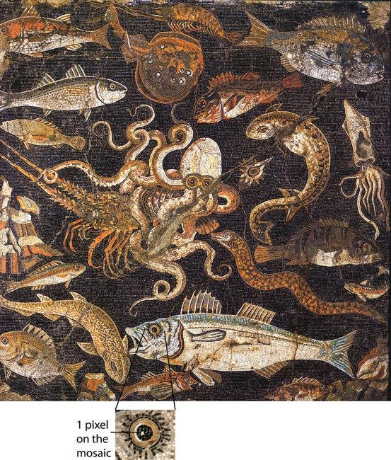
Images have structure. They have a certain arrangement of small and large objects. The large objects are often composites of small objects. The Roman mosaic from the House VIII.1.16 in Pompeii, the House of Five Floors, has incredible structure (Figure 1.1). It has lifelike images of a bird on a reef, fishes, an electric eel, a shrimp, a squid, an octopus, and a rock lobster. It illustrates Aristotle’s natural history account of a struggle between a rock lobster and an octopus. In fact, the species are identifiable and are common to certain bays in the Italian coast, a remarkable example of early biological imaging.
It is a mosaic of uniformly sized square colored tiles. Each tile is the smallest picture element, or pixel, of the mosaic. At a certain appropriate viewing distance from the mosaic, the individual pixels cannot be distinguished, or resolved, and what is a combination of individual tiles looks solid or continuous, taking the form of a fish, or lobster, or octopus. When viewed closer than this distance, the individual tiles or pixels become apparent (see Figure 1.1); the image is pixelated Beyond viewing it from the distance that is the height of the person standing on the mosaic, pixelation in this scene was probably further reduced by the shallow pool of water that covered it in the House of Five Floors.
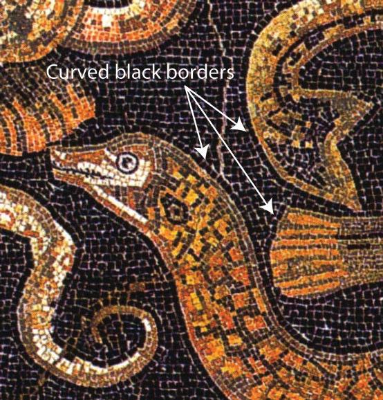
The order in which the image elements come together, or render, also describes the image structure. This mosaic was probably constructed by tiling the different objects in the scene, then surrounding the objects with a single layer of tiles of the black background (Figure 1.2), and finally filling in the background with parallel rows of black tiles. This form of image construction is object-order rendering. The background rendering follows the rendering of the objects. Vector graphic images use object-ordered rendering. Vector graphics define the object mathematically with a set of vectors and render it in a scene, with the background and other objects rendered separately.
Vector graphics are very useful because any number of pixels can represent the mathematically defined objects. This is why programs, such as Adobe Illustrator, with vector graphics for fonts and illustrated objects are so useful: the number (and, therefore, size) of pixels that represent the image is chosen by the user and depends on the type of media that will display it. This number can be set so that the fonts and objects never have to appear pixelated. Vector graphics are resolution independent; scaling the object to any size will not lose its sharpness from pixelation.
Another way to make the mosaic would be to start from the top upper left of the mosaic and start tiling in rows. One row near the top of the mosaic contains parts of three fishes, a shrimp, and the background. This form of image structure is image-order rendering. Many scanning systems construct images using this form of rendering. A horizontal scan line is a raster. Almost all computer displays and televisions are raster based. They display a rasterized grid of data, and because the data are in the form of bits (see Section 2.2), it is a bitmap image. As described later, bitmap graphics are resolution dependent; that is, as they scale larger, the pixels become larger, and the images become pixelated.
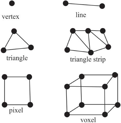
Even though pixels are the smallest discrete unit of the picture, it does have structure. The fundamental unit of visualization is the cell (Figure 1.3). A pixel is a two-dimensional (2D) cell described by an ordered list of four points (its corners or vertices), and geometric constraints make it square. In three-dimensional (3D) images, the smallest discrete unit of the volume is the voxel. A voxel is the 3D cell described by an ordered list of eight points (its vertices), and geometrics constraints make it a cube.
Imaging Life: Image Acquisition and Analysis in Biology and Medicine, First Edition. Lawrence R. Griffing. © 2023 John Wiley & Sons, Inc. Published 2023 by John Wiley & Sons, Inc.
Companion Website: www.wiley.com/go/griffing/imaginglife
Figure 1.1 The fishes mosaic (second century BCE) from House VII.2.16, the House of Five Floors, in Pompeii. The lower image is an enlargement of the fish eye, showing that light reflection off the eye is a single tile, or pixel, in the image. Photo by Wolfgang Rieger, http://commons.wikimedia.org/wiki/File:Pompeii_-_ Casa_del_Fauno_-_MAN.jpg and is in the public domain (PD-1996).
Figure 1.2 Detail from Figure 2.1. The line of black tiles around the curved borders of the eel and the fish are evidence that the mosaic employs object-order rendering.
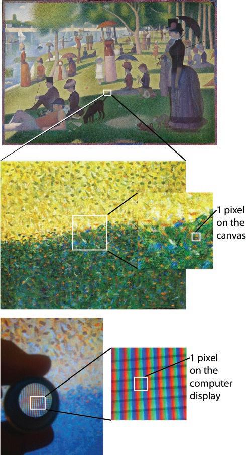
Color is a subpixel component of electronic displays; printed material; and, remarkably, some paintings. Georges Seurat (1859–1891) was a famous French post-impressionist painter. Seurat communicated his impression of a scene by constructing his picture from many small dabs or points of paint (Figure 1.4); he was a pointillist. However, each dab of paint is not a pixel. Instead, when standing at the appropriate viewing distance, dabs of differently colored paint combine to form a new color. Seurat pioneered this practice of subpixel color. Computer displays use it, each pixel being made up of stripes (or dots) of red, green, and blue color (see Figure 1.4). The intensity of the different stripes determines the displayed color of the pixel.
For many printed images, the half-tone cell is the pixel. A halftone cell contains an array of many black and white dots or dots of different colors (see Figure 1.10); the more dots within the halftone cell, the more shades of gray or color that are possible. Chapter 2 is all about how different pixel values produce different shades of gray or color.
Figure 1.3 Cell types found in visualization systems that can handle two- and three-dimensional representation. Diagram by L. Griffing.
Figure 1.4 This famous picture A Sunday Afternoon on the Island of La Grande Jatte (1884–1886) by Georges Seurat is made up of small dots or dabs of paint, each discrete and with a separate color. Viewed from a distance, the different points of color, usually primary colors, blend in the mind of the observer and create a canvas with a full spectrum of color. The lower panel shows a picture of a liquid crystal display on a laptop that is displaying a region of the Seurat painting magnified through a lens. The view through the lens reveals that the image is composed of differently illuminated pixels made up of parallel stripes of red, green, and blue colors. The upper image is from https://commons.wikimedia.org/wiki/File:A_Sunday_on_La_ Grande_Jatte,_Georges_Seurat,_1884.jpg. Lower photos by L. Griffing.
1.2 The Resolving Power of a Camera or Display Is the Spatial Frequency of Its Pixels
In biological imaging, we use powerful lenses to resolve details of far away or very small objects. The round plant protoplasts in Figure 1.5 are invisible to the naked eye. To get an image of them, we need to use lenses that collect a lot of light from a very small area and magnify the image onto the chip of a camera. Not only is the power of the lens important but also the power of the camera. Naively, we might think that a powerful camera will have more pixels (e.g., 16 megapixels [MP]) on its chip than a less powerful one (e.g., 4 MP). Not necessarily! The 4-MP camera could actually be more powerful (require less magnification) if the pixels are smaller. The size of the chip and the pixels in the chip matter.
The power of a lens or camera chip is its resolving power, the number of pixels per unit length (assuming a square pixel). It is not the number of total pixels but the number of pixels per unit space, the spatial frequency of pixels. For example, the eye on the bird in the mosaic in Figure 1.1 is only 1 pixel (one tile) big. There is no detail to it. Adding more tiles to give the eye some detail requires smaller tiles, that is, the number of tiles within that space of the eye increases – the spatial frequency of pixels has to increase. Just adding more tiles of the original size will do no good at all. Common measures of spatial frequency and resolving power are pixels per inch (ppi) or lines per millimeter (lpm – used in printing).
Another way to think about resolving power is to take its inverse, the inches or millimeters per pixel. Pixel size, the inverse of the resolving power, is the image resolution. One bright pixel between two dark pixels resolves the two dark pixels. Resolution is the minimum separation distance for distinguishing two objects, dmin. Resolving power is 1/dmin
Note: Usage of the terms resolving power and resolution is not universal. For example, Adobe Photoshop and Gimp use resolution to refer to the spatial frequency of the image. Using resolving power to describe spatial frequencies facilitates the discussion of spatial frequencies later.
As indicated by the example of the bird eye in the mosaic and as shown in Figure 1.5, the resolving power is as important in image display as it is in detecting the small features of the object. To eliminate pixelation detected by eye, the resolving power of the eye should be less than the pixel spatial frequency on the display medium when viewed from an appropriate viewing distance. The eye can resolve objects separated by about 1 minute (one 60th) of 1 degree of the almost 140-degree field of view for binocular vision. Because things appear smaller with distance, that is, occupy a

Figure 1.5 Soybean protoplasts (cells with their cell walls digested away with enzymes) imaged with differential interference contrast microscopy and displayed at different resolving powers. The scale bar is 10 μm long. The mosaic pixelation filter in Photoshop generated these images. This filter divides the spatial frequency of pixels in the original by the “cell size” in the dialog box (filter > pixelate > mosaic). The original is 600 ppi. The 75-ppi images used a cell size of 8, the 32-ppi image used a cell size of 16, and the 16-ppi image used a cell size of 32. Photo by L. Griffing.
Table 1.1 Laptop, Netbook, and Tablet Monitor Sizes, Resolving Power, and Resolution.
smaller angle in the field of view, even things with large pixels look non-pixelated at large distances. Hence, the pixels on roadside signs and billboards can have very low spatial frequencies, and the signs will still look non-pixelated when viewed from the road.
Appropriate viewing distances vary with the display device. Presumably, the floor mosaic (it was an interior shallow pool, so it would have been covered in water) has an ideal viewing distance, the distance to the eye, of about 6 feet. At this distance, the individual tiles would blur enough to be indistinguishable. For printed material, the closest point at which objects come into focus is the near point, or 25 cm (10 inches) from your eyes. Ideal viewing for typed text varies with the size of font but is between 25 and 50 cm (10 and 20 inches). The ideal viewing distance for a television display, with 1080 horizontal raster lines, is four times the height of the screen or two times the diagonal screen dimension. When describing a display or monitor, we use its diagonal dimension (Table 1.1). We also use numbers of pixels. A 14-inch monitor with the same number of pixels as a 13.3-inch monitor (2.07 × 10⁶ in Table 1.1) has larger pixels, requiring a slightly farther appropriate viewing distance. Likewise, viewing a 24-inch HD 1080 television from 4 feet is equivalent to viewing a 48-inch HD 1080 television from 8 feet.
There are different display standards, based on aspect ratio, the ratio of width to height of the displayed image (Table 1.2). For example, the 15.6-inch monitors in Table 1.1 have different aspect ratios (Apple has 8:5 or 16:10, while Windows has 16:9). They also use different standards: a 1920 × 1200 monitor uses the WUXGA standard (see Table 1.2), and the 3840 × 2160 monitor uses the UHD-1 standard (also called 4K, but true 4K is different; see Table 1.2). The UHD-1 monitor has half the pixel size of the WUXGA monitor. Even though these monitors have the same diagonal dimension, they have different appropriate viewing distances. The standards in Table 1.2 are important when generating video (see Sections 5.8 and 5.9) because different devices have different sizes of display (see Table 1.1). Furthermore, different video publication sites such as YouTube and Facebook and professional journals use standards that fit multiple devices, not just devices with high resolving power. We now turn to this general problem of different resolving powers for different media.
1.3 Image Legibility Is the Ability to Recognize Text in an Image by Eye
Image legibility, or the ability to recognize text in an image, is another way to think about resolution (Table 1.3). This concept incorporates not only the resolution of the display medium but also the resolution of the recording medium, in this case, the eye. Image legibility depends on the eye’s inability to detect pixels in an image. In a highly legible image, the eye does not see the individual pixels making up the text (i.e., the text “looks” smooth). In other words, for text to be highly legible, the pixels should have a spatial frequency near to or exceeding the resolving power of the eye.
At near point (25 cm), it is difficult for the eye to resolve two points separated by 0.1 mm or less. An image that resolves 0.1 mm pixels has a resolving power of 10 pixels per mm (254 ppi). Consequently, a picture reproduced at 300 ppi would
Table 1.2 Display Standards.
Aspect Ratio (Width:Height in Pixels)
4:3 8:5 (16:10) 16:9 Various QVGA
320 × 240 CGA
320 × 200
SIF/CIF
384 × 288
352 × 288
VGA
640 × 480 WVGA (5:3) 800 × 480 WVGA 854 × 480
PAL
768 × 576 PAL 1024 × 576
SVGA
800 × 600 WSVGA 1024 × 600 XGA 1024 × 786 WXGA 1280 × 800 HD 720 1280 × 720
SXGA+ 1400 × 1050 WXGA+ 1680 × 1050 HD 1080 1920 × 1080 SXGA (5:4) 1280 × 1024
UXGA 1600 × 1200 WUXGA 1920 × 1200 2K (17:9) 2048 × 1080 UWHD (21:9) 2560 × 1080 QXGA 2048 × 1536 WQXGA 1560 × 1600 WQHD 2560 × 1440 QSXGA (5:4) 2560:2048
UHD-1 3840 × 2160 UWQHD (21:9) 3440 × 1440 4K (17:9) 4096 × 2160 8K 7680 × 4320
Table 1.3 Image Legibility.
Power
200 8 Excellent High clarity
100 4 Good Clear enough for prolonged study
50 2 Fair Identity of letters questionable
25 1 Poor Writing illegible lpm, lines per inch; ppi, pixels per inch.
have excellent text legibility (see Table 1.3). However, there are degrees of legibility; some early computer displays had a resolving power, also called dot pitch, of only 72 ppi. As seen in Figure 1.5, some of the small particles in the cytoplasm of the cell vanish at that resolving power. Nevertheless, 72 ppi is the borderline between good and fair legibility (see Table 1.3) and provides enough legibility for people to read text on the early computers.
The average computer is now a platform for image display. Circulation of electronic images via the web presents something of a dilemma. What should the resolving power of web-published images be? To include computer users who use old displays,
Table 1.4 Resolving Power Required for Excellent Images from Different Media.
Imaging Media
Portable computer
Standard print text
Printed image
Film negative scan
Black and white line drawing
Resolving Power (ppi)
90–180
200
300 (grayscale)
350–600 (color)
1500 (grayscale)
3000 (color)
1500 (best done with vector graphics)
the solution is to make it equal to the lowest resolving power of any monitor (i.e., 72 ppi). Images at this resolving power also have a small file size, which is ideal for web communication. However, most modern portable computers have larger resolving powers (see Table 1.1) because as the numbers of horizontal and vertical pixels increase, the displays remain a physical size that is portable. A 72-ppi image displayed on a 144-ppi screen becomes half the size in each dimension. Likewise, high-ppi images become much bigger on low-ppi screens. This same problem necessitates reduction of the resolving power of a photograph taken with a digital camera when published on the web. A digital camera may have 600 ppi as its default output resolution. If a web browser displays images at 72 ppi, the 600-ppi image looks eight times its size in each dimension.
This brings us to an important point. Different imaging media have different resolving powers. For each type of media, the final product must look non-pixelated when viewed by eye (Table 1.4). These values are representative of those required for publication in scientific journals. Journals generally require grayscale images to be 300 ppi, and color images should be 350–600 ppi. The resolving power of the final image is not the same as the resolving power of the newly acquired image (e.g., that on the camera chip). The display of images acquired on a small camera chip requires enlargement. How much is the topic of the next section.
1.4 Magnification Reduces Spatial Frequencies While Making Bigger Images
As discussed earlier, images acquired at high resolving power are quite large on displays that have small resolving power, such as a 72-ppi web page. We have magnified the image! As long as decreasing the spatial frequency of the display does not result in pixelation, the process of magnification can reveal more detail to the eye. As soon as the image becomes pixelated, any further magnification is empty magnification. Instead of seeing more detail in the image, we just see bigger image pixels.
In film photography, the enlargement latitude is a measure of the amount of negative enlargement before empty magnification occurs and the image pixel, in this case the photographic grain, becomes obvious. Likewise, for chip cameras, it is the amount of enlargement before pixelation occurs. Enlargement latitude is
E= R/ L,
(1.1)
in which E is enlargement magnification, R is the resolving power (spatial frequency of pixels) of the original, and L is the acceptable legibility.
For digital cameras, it is how much digital zoom is acceptable (Figure 1.6). A sixfold magnification reducing the resolving power from 600 to 100 ppi produces interesting detail: the moose calves become visible, and markings on the female become clear. However, further magnification produces pixelation and empty magnification. Digital zoom magnification is common in cameras. It is very important to realize that digital zoom reduces the resolving power of the image. For scientific applications, it is best to use only optical zoom in the field and then perform digital zoom when analyzing or presenting the image.
The amount of final magnification makes a large difference in the displayed image content. The image should be magnified to the extent that the subject or region of interest (ROI) fills the frame but without pixelation. The ROI is the image area of the most importance, whether for display, analysis, or processing. Sometimes showing the environmental context of a feature is important. Figure 1.7 is a picture of a female brown bear being “herded” by or followed by a male in the spring (depending