Comparative life cycle assessment of rainbow trout ( Oncorhynchus mykiss ) farming at two stocking densities in a low-tech aquaponic system Francesco Bordignon
Current Developments in Biotechnology and Bioengineering: Smart Solutions for Wastewater: Road-mapping the Transition to Circular Economy Giorgio Mannina
No part of this publication may be reproduced or transmitted in any form or by any means, electronic or mechanical, including photocopying, recording, or any information storage and retrieval system, without permission in writing from the publisher. Details on how to seek permission, further information about the Publisher’s permissions policies and our arrangements with organizations such as the Copyright Clearance Center and the Copyright Licensing Agency, can be found at our website: www.elsevier.com/permissions.
This book and the individual contributions contained in it are protected under copyright by the Publisher (other than as may be noted herein).
Notices
Knowledge and best practice in this field are constantly changing. As new research and experience broaden our understanding, changes in research methods, professional practices, or medical treatment may become necessary.
Practitioners and researchers must always rely on their own experience and knowledge in evaluating and using any information, methods, compounds, or experiments described herein. In using such information or methods they should be mindful of their own safety and the safety of others, including parties for whom they have a professional responsibility.
To the fullest extent of the law, neither the Publisher nor the authors, contributors, or editors, assume any liability for any injury and/or damage to persons or property as a matter of products liability, negligence or otherwise, or from any use or operation of any methods, products, instructions, or ideas contained in the material herein.
British Library Cataloguing-in-Publication Data
A catalogue record for this book is available from the British Library
Library of Congress Cataloging-in-Publication Data
A catalog record for this book is available from the Library of Congress
ISBN: 978-0-08-099986-9
For information on all Elsevier publications visit our website at https://www.elsevier.com/
Typeset by Thomson Digital
Preface
There can be no doubt that nuclear magnetic resonance (NMR) spectroscopy is now a very well developed analytical tool and one that continues to expand in its capabilities and application. This is manifest in the fact that many NMR subdisciplines have now established themselves as separate research fields in their own right, with practitioners of NMR often finding themselves specialising in one of these areas. Common, loosely defined fields might include ‘small’ molecules, bio-macromolecules and metabolomics, aside from solid-state NMR, which itself nowadays largely partitions to materials science and biomolecules. Likewise, NMR texts tend to focus on one of these disciplines as it becomes increasingly difficult to do adequate justice to more than one in a single book. In keeping with the previous two editions, this text continues its focus on solution-state NMR techniques for the study of small molecules. In addition, this third edition extends to medicinal chemistry related applications, reflecting the increasing use of small molecule NMR at the life-sciences interface, and as such includes a completely new chapter on ligand–protein interactions. A second new chapter, presenting a model case study, illustrates how the most common NMR methods may be combined in the structure elucidation of a single compound. The earlier introductory material in the book has also been expanded, notably with regard to dynamic NMR effects, and all chapters have been updated to reflect modern instrument developments, current methodology and new experimental techniques, as outlined subsequently.
The Chapter Introducing High-Resolution NMR develops the basic concepts and principles of NMR, including pulse excitation and spin relaxation. This chapter has been extended significantly with a new section on dynamic NMR spectroscopy. This describes the influence of dynamic effects on NMR spectra, introduces the concepts of NMR timescales and defines fast and slow exchange processes. It also describes the use of lineshape analysis and magnetisation transfer experiments for the measurement of equilibrium exchange rates. The chapter describing Practical Aspects of High-Resolution NMR focuses on the practicalities of executing NMR experiments and has been updated to include recent technological developments, including nitrogen-cooled cryogenic probeheads. The chapter on One-Dimensional Techniques introduces the primary 1D NMR techniques and for this edition discussions on quantitative NMR (qNMR) have been extended to reflect the increasing use of NMR as a primary technique for defining compound purity. The following chapter Introducing Two-Dimensional and Pulsed Field Gradient NMR has been revised slightly from that of previous editions and now focuses solely on introducing the principles and practicalities of 2D NMR and of pulsed field gradients (PFGs). The chapter also includes non-uniform sampling for more rapid data collection and concludes by introducing the concept of single-scan NMR, the ultimate in fast data acquisition. The chapter Correlations Through the Chemical Bond I: Homonuclear Shift Correlation then focuses on techniques for establishing correlations between homonuclear spins. The theme of through-bond correlations continues with Correlations Through the Chemical Bond II: Heteronuclear Shift Correlation which describes heteronuclear correlation techniques. This chapter has been restructured in this edition to emphasise the favoured use of heteronuclear single-quantum correlation (HSQC) over heteronuclear multiple-quantum correlation (HMQC) nowadays, with the later retained partly as a lead into to the very important and closely related heteronuclear multiple-bond correlation (HMBC) technique. The sections covering HMBC have also been extended to consider new variants, including those suitable for measuring long-range, proton-carbon coupling constants and for the investigation of proton-sparse molecules. The chapter concludes with an introduction to the concept of parallel acquisition NMR in which multiple NMR receivers are employed. Whilst uncommon at present, these methods are potentially significant for future developments leading to more efficient data acquisition. The chapter Separating Shifts and Couplings: J-Resolved and Pure Shift Spectroscopy introduces classical J-resolved spectroscopy and also contains a substantial new section describing pure shift broadband decoupled proton NMR. The chapter describing Correlations Through Space: The Nuclear Overhauser Effect provides an introduction to the basic principles of the NOE. Following this, the practical section has been significantly restructured to emphasise the dominance of the transient NOE (most often measured by NOESY) over the older steady-state difference experiments for measuring proton–proton NOEs. The section on heteronuclear Overhauser effects has been extended to include methods for 19F–1H NOEs, included to match the growing interest in fluorine chemistry. The section on 2D exchange spectroscopy (EXSY) has also been revised to integrate with the new dynamics section found in the chapter Introducing
High-Resolution NMR. Finally in this chapter, a new section on residual dipolar couplings (RDCs) and their use in defining stereochemistry has been included, with practical discussions and example applications. The chapter Diffusion NMR Spectroscopy describes techniques for studying molecular self-diffusion and has been updated to include the latest consideration of convection and its complicating effects. It also includes coverage of some recent and pragmatic approaches for correlating measured diffusion coefficients with molecular size. The chapter describing Protein-Ligand Screening by NMR presents a completely new topic with a focus on methods for studying the interactions of small molecule ligands with macromolecular targets, principally proteins. NMR spectroscopy is increasingly applied in drug discovery programmes and in the development of small molecule probes of biochemical pathways, meaning these techniques are finding increasing use in chemical laboratories that interface with biological science. After an introduction to relevant binding equilibria, various techniques are presented which focus on the response of the small molecule on binding to a target. The most popular NMR methods are described, including relaxation editing, STD, water-LOGSY, exchange-transferred NOEs and the use of competition experiments. Alternative methods employing observation of protein responses are also considered. The chapter on Experimental Methods describes elements of NMR that are used to build modern pulse sequences and has been updated to reflect recent developments and to include older methodologies that have become more established in their roles. Descriptions of hyperpolarisation have been extended to include para-hydrogen based methods (PHIP) in addition to dynamic nuclear polarisation (DNP). The final chapter Structure Elucidation and Spectrum Assignment is also a new addition to this third edition and seeks to exemplify the combined application of some of the primary methods described in the book to the structure elucidation of a moderately complex small molecule. This case study illustrates how these techniques may be applied in a stepwise approach to systematically build a molecular structure and to define its stereochemistry from 1D and 2D NMR data, also highlighting how less-commonly employed techniques might be used in the assignment of more complex data sets. The book concludes with an updated glossary of terms and acronyms that find common use in the field. In producing the new chapters and sections for this edition, I have once again benefitted from the generous input of many people. From the Chemistry Department in Oxford, I thank my colleagues in the NMR facility Drs Nick Rees and Barbara Odell, and from the University of Auckland Dr Ivanhoe Leung, for providing useful comments and suggestions on new drafts. I am similarly grateful to many group leaders and their research students in the Oxford Chemistry Department for making novel compounds available with which to illustrate the application of various experimental techniques, in particular Profs Stuart Conway, Ben Davis, Philip Mountford, Chris Schofield and Martin Smith. For the provision of original data sets used to prepare figures, I thank Prof Christina Redfield (Department of Biochemistry, University of Oxford), Prof Simon Duckett (Department of Chemistry, University of York), Dr Eriks Kupcˇe (Bruker Biospin UK Ltd), Dr Ignacio Perez-Victoria (formally of Department of Chemistry, University of Oxford) and again Dr Nick Rees. For making their software packages freely available, I thank Prof Hans Reich (University of Wisconsin) for the WinDNMR lineshape simulation program and Prof Alex Bain (McMaster University) for the CIFIT magnetisation transfer fitting program. I am also grateful to Katey Birtcher, Jill Cetel and Anitha Sivaraj of Elsevier for their assistance and patience during the development and production of this new edition.
As previously, those to which I am most grateful are my wife Rachael and daughter Emma for once again demonstrating their continued tolerance and support throughout this project. One might imagine each new edition should be easier and perhaps quicker to complete than the last, but somehow that never seems to be the case, for which I can only apologise.
From the initial observation of proton magnetic resonance in water [1] and in paraffin [2], the discipline of nuclear magnetic resonance (NMR) has seen unparalleled growth as an analytical method and now, in numerous different guises, finds application in chemistry, biology, medicine, materials science and geology. The founding pioneers of the subject, Felix Bloch and Edward Purcell, were recognised with a Nobel Prize in 1952 ‘for their development of new methods for nuclear magnetic precision measurements and discoveries in connection therewith’. The maturity of the discipline has since been recognised through the awarding of Nobel Prizes to two of the pioneers of modern NMR methods and their application, Richard Ernst (1991, ‘for his contributions to the development of the methodology of high resolution NMR spectroscopy’) and Kurt Wüthrich (2002, ‘for his development of NMR spectroscopy for determining the three-dimensional structure of biological macromolecules in solution’). Despite its inception in the laboratories of physicists, it is in chemical and biochemical laboratories that NMR spectroscopy has found greatest use. To put into context the range of techniques now available in the modern chemical laboratory, including those described in this book, we begin with a short overview of the evolution of high-resolution (solution-state) NMR spectroscopy and some of the landmark developments that have shaped the subject.
1.1 THE DEVELOPMENT OF HIGH-RESOLUTION NMR
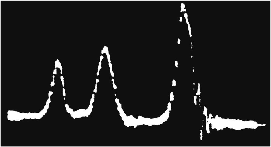
It is almost 70 years since the first observations of NMR were made in both solid and liquid samples, from which the subject has evolved to become the principal structural technique of the research chemist, alongside mass spectrometry. During this time, there have been a number of key advances in high-resolution NMR that have guided the development of the subject [3–5] (Table 1.1) and consequently the work of chemists and their approaches to structure elucidation. The seminal step occurred during the early 1950s when it was realised that the resonant frequency of a nucleus is influenced by its chemical environment, and that one nucleus could further influence the resonance of another through intervening chemical bonds. Although these observations were seen as unwelcome chemical complications by the investigating physicists, a few pioneering chemists immediately realised the significance of these chemical shifts and spin–spin couplings within the context of structural chemistry. The first high-resolution proton NMR spectrum (Fig. 1.1) clearly demonstrated how the features of an NMR spectrum, in this case chemical shifts, could be directly related to chemical structure and it is from this that NMR has evolved to attain the significance it holds today.
The 1950s also saw a variety of instrumental developments that were to provide the chemist with even greater chemical insight. These included the use of sample spinning for averaging to zero field inhomogeneities which provided a substantial increase in resolution, so revealing fine splittings from spin–spin coupling. Later, spin decoupling was able to provide more specific information by helping the chemists understand these interactions. With these improvements, sophisticated relationships could be developed between chemical structure and measurable parameters, leading to such realisations as the dependence of vicinal coupling constants on dihedral angles (the now well-known Karplus relationship). The inclusion of computers during the 1960s was also to play a major role in enhancing the influence of NMR on the chemical community. The practice of collecting the same continuous wave spectrum repeatedly and combining them with a CAT (computer of average transients) led to significant gains in sensitivity and made the observation of smaller sample quantities a practical realisation. When the idea of stimulating all spins simultaneously with a single pulse of
TABLE 1.1 A Summary of Some Key Developments that have had a Major Influence on the Practice and Application of High-Resolution NMR Spectroscopy in Chemical Research
Decade Notable Advances
1940s First observation of NMR in solids and liquids (1945)
1950s Development of chemical shifts and spin–spin coupling constants as structural indicators
1960s Use of signal averaging for improving sensitivity
Application of the pulse FT approach
The NOE employed in structural investigations
1970s Use of superconducting magnets and their combination with the FT approach
Computer-controlled instrumentation
1980s Development of multipulse and 2D NMR techniques
Automated spectroscopy
1990s Routine application of pulsed field gradients for signal selection
Development of coupled analytical methods (eg LC-NMR)
2000s Use of high-sensitivity helium-cooled cryogenic probes
Routine availability of actively shielded magnets for reduced stray fields
Development of microscale tube and flow probes
2010+ Adoption of fast data acquisition methods
Use of high-sensitivity nitrogen-cooled cryogenic probes
Use of multiple receivers…?
radiofrequency, collecting the time domain response and converting this to the required frequency domain spectrum by a process known as Fourier transformation (FT) was introduced, more rapid signal averaging became possible. This approach provided an enormous increase in the signal-to-noise ratio, and was to change completely the development of NMR spectroscopy. The mid-1960s also saw the application of the nuclear Overhauser effect (NOE) to conformational studies. Although described during the 1950s as a means of enhancing the sensitivity of nuclei through the simultaneous irradiation of electrons, the NOE has since found widest application in sensitivity enhancement between nuclei, or in the study of the spatial proximity of nuclei, and remains one of the most important tools of modern NMR. By the end of the 1960s, the first commercial FT spectrometer was available, operating at 90 MHz for protons. The next great advance in field strengths was provided by the introduction of superconducting magnets during the 1970s, which were able to provide significantly higher fields than the electromagnets previously employed. These, combined with the FT approach, made the observation of carbon-13 routine and provided the organic chemist with another probe of molecular structure. This also paved the way for the routine observation of a whole variety of previously inaccessible nuclei of low natural abundance and low magnetic moment. It was also in the early 1970s that the concept of spreading the information contained within the NMR spectrum into two separate frequency dimensions was proposed in a lecture. However, because of instrumental limitations, the quality of the first 2D spectra were considered too poor to be published, and not until the mid-1970s, when instrument stability had improved and developments in computers made the necessary complex calculations feasible, did the development of 2D methods begin in earnest. These methods, together with the various multipulse 1D methods that
with permission from Ref. [6], Copyright 1951, American Institute
FIGURE 1.1 The first ‘high-resolution’ proton NMR spectrum, recorded at 30 MHz, displaying the proton chemical shifts in ethanol. (Source: Reprinted
of Physics.)
also became possible with the FT approach, were not to have significant impact on the wider chemical community until the 1980s, from which point their development was nothing less than explosive. This period saw an enormous number of new pulse techniques presented which were capable of performing a variety of ‘spin gymnastics’ and so provided the chemist with ever more structural data, on smaller sample quantities and in less time. No longer was it necessary to rely on empirical correlations of chemical shifts and coupling constants with structural features to identify molecules, instead a collection of spin interactions (through-bond, through-space, chemical exchange) could be mapped and used to determine structures more reliably and more rapidly. The evolution of new pulse methods continued throughout the 1990s, alongside which emerged a fundamentally different way of extracting the desired information from molecular systems. Pulsed field gradient–selected experiments have now become routine structural tools, providing better quality spectra, often in shorter times, than was previously possible. These came into widespread use not so much from a theoretical breakthrough (their use for signal selection was first demonstrated in 1980) but again as a result of progressive technological developments defeating practical difficulties. Similarly, the emergence of coupled analytical methods, such as liquid chromatography and NMR (LC-NMR), came about after the experimental complexities of interfacing these very different techniques was overcome, and these methods have established themselves for the analysis of complex mixtures, albeit as a niche area. Developments in probe technologies over recent decades have allowed wider adoption of probeheads containing coils and preamplifiers that are cryogenically cooled by either cold helium or nitrogen. This reduces system noise significantly and so enhances detection signal-to-noise ratios. Probe coil miniaturisation has also provided a boost in the signal-to-noise ratio for mass limited samples, and the marrying of this with cryogenic technology nowadays offers one of the most effective routes to higher detection sensitivity. Instrument miniaturisation has also been a constant theme, leading to smaller and more compact consoles driven by developments in solid-state electronics. Likewise, actively shielded superconducting magnets with significantly reduced stray fields are now standard, making the siting of instruments considerably easier and far less demanding on space. For example, first-generation unshielded magnets operating at 500 MHz possessed stray fields that would extend to over 3 m horizontally from the magnet centre when measured at the 0.5 mT (5 G) level, the point beyond which disturbances to the magnetic field are not considered problematic. Nowadays, latest-generation shielded magnets have this line sited at somewhat less than 1 m from the centre and only a little beyond the magnet dewar itself. This is achieved through the use of compensating magnet coils that seek to counteract the stray field generated outside the magnet assembly. Other developments have allowed recycling of the liquid cryogens needed to maintain the superconducting state of the magnet through the reliquification of helium and nitrogen gas. Recycling of helium in this manner is already established for imaging magnets but has posed considerable challenges in the context of high-resolution NMR measurements which have only relatively recently been overcome. More extreme miniaturisation of magnets has come about through the use of rare earth metals formed as Halbach array magnets. These ambient temperature devices require no cryogens and provide fields suitable for instruments operating below proton frequencies of 100 MHz. Their compact sizes have allowed the creation of low-field bench-top NMR spectrometers that find use in simple reaction screening or in educational roles, for example. Very recent developments have again taken their inspiration from imaging methodology and have seen the concept of multiple receivers applied to high-resolution NMR. As the name suggests, this allows simultaneous detection of NMR responses from multiple nuclei and has the potential to streamline data acquisition. This is an area still in its infancy and its impact on data collection protocols remains to be seen.
Modern NMR spectroscopy is now a highly developed and technologically advanced subject. With so many advances in NMR methodology in recent years it is understandably an overwhelming task for the research chemist, and even the dedicated spectroscopist, to appreciate what modern NMR has to offer. This text aims to assist in this task by presenting the principal modern NMR techniques and exemplifying their application.
1.2 MODERN HIGH-RESOLUTION NMR AND THIS BOOK
There can be little doubt that NMR spectroscopy now represents the most versatile and informative spectroscopic technique employed in the modern chemical research laboratory, and that an NMR spectrometer represents one of the largest single investments in analytical instrumentation the laboratory is likely to make. For both these reasons it is important that the research chemist is able to make the best use of the available spectrometer(s) and to harness modern developments in NMR spectroscopy in order to promote their chemical or biochemical investigations. Even the most basic modern spectrometer is equipped to perform a myriad of pulse techniques capable of providing the chemist with a variety of data on molecular structure and dynamics. Not always do these methods find their way into the hands of the practising chemist, remaining instead in the realms of the specialist, obscured behind esoteric acronyms or otherwise unfamiliar NMR jargon. Clearly this should not be so and the aim of this book is to gather up the most useful of these modern NMR methods and present them to the wider audience who should, after all, find greatest benefit from their application.
The approach taken throughout is non-mathematical and is based firmly on using pictorial descriptions of NMR phenomena and methods wherever possible. In preparing and updating this work, I have attempted to keep in mind what I perceive to be the requirements of three major classes of potential readers:
1. those who use solution-state NMR as a tool in their own research, but have little or no direct interaction with the spectrometer;
2. those who have undertaken training in directly using a spectrometer to acquire their own data, but otherwise have little to do with the upkeep and maintenance of the instrument; and
3. those who make use spectrometers and are responsible for the day-to-day upkeep of the instrument. This may include NMR laboratory managers, although in some cases users may not consider themselves dedicated NMR spectroscopists.
The first of these could well be research chemists and students in an academic or industrial environment who need to know what modern techniques are available to assist them in their efforts, but otherwise feel they have little concern for the operation of a spectrometer. Their data are likely to be collected under fully-automated conditions, or provided by a central analytical facility. The second may be a chemist in an academic environment who has hands-on access to a spectrometer and has his or her own samples which demand specific studies that are perhaps not available from fully automated instrumentation. The third class of reader may work in smaller chemical companies or academic chemistry departments that have invested in NMR instrumentation but may not employ a dedicated NMR spectroscopist for its upkeep, depending instead on, say, an analytical or synthetic chemist for this. This, it appears (in the United Kingdom at least), is often the case for new start-up chemical companies. NMR laboratory managers may also find the text a useful reference source. With these in mind, the book contains a fair amount of practical guidance on both the execution of NMR experiments and the operation and upkeep of a modern spectrometer. Even if you see yourself in the first of the above categories, some rudimentary understanding of how a spectrometer collects the data of interest and how a sequence produces, say, the 2D correlation spectrum awaiting analysis on your computer, can be enormously helpful in correctly extracting the information it contains or in identifying and eliminating artefacts that may arise from instrumental imperfections or the use of less-than-optimal conditions for your sample. Although not specifically aimed at dedicated spectroscopists, the book may still contain new information or may serve as a reminder of what was once understood but has somehow faded away. The text should be suitable for (UK) graduate-level courses on NMR spectroscopy, and sections of the book may also be appropriate for use in advanced undergraduate courses. The book does not, however, contain descriptions of basic NMR phenomena such as chemical shifts and coupling constants, neither does it contain extensive discussions on how these may be correlated with chemical structures. These topics are already well documented in various introductory texts [7–13] and it is assumed that the reader is already familiar with such matters. Likewise, the book does not seek to provide a comprehensive physical description of the processes underlying the NMR techniques presented; the books by Hore et al. [14] and Keeler [15] present this at an accessible yet rigorous level. Although the chapter on Protein Ligand Screening by NMR discusses NMR methods for the study of protein–small-molecule interactions, this text does not discuss techniques for the assignment and structure elucidation of proteins themselves, topics which are also covered in dedicated texts [16–18]
1.2.1 What This Book Contains
The aim of this text is to present the most important NMR methods used for chemical structure elucidation, to explain the information they provide, how they operate and to provide some guidance on their practical implementation. The choice of experiments is naturally a subjective one, partially based on personal experience, but also taking into account those methods most commonly encountered in the chemical literature and those recognised within the NMR community as being most informative and of widest applicability. The operation of many of these is described using pictorial models (equations appear infrequently, and are only included when they serve a specific purpose) so that the chemist can gain some understanding of the methods they are using without recourse to uninviting mathematical descriptions. The sheer number of available NMR methods may make this seem an overwhelming task, but in reality most experiments are composed of a smaller number of comprehensible building blocks pieced together, and once these have been mastered an appreciation of more complex sequences becomes a far less daunting task. For those readers wishing to pursue a particular topic in greater detail, the original references are given but otherwise all descriptions are self-contained.
The following chapter Introducing High-Resolution NMR introduces the basic model used throughout the book for the description of NMR methods and describes how this provides a simple picture of the behaviour of chemical shifts and spin–spin couplings during pulse experiments. This model is then used to visualise nuclear spin relaxation, a feature of central importance for the optimum execution of all NMR experiments (indeed, it seems early attempts to observe NMR failed most probably because of a lack of understanding at the time of the relaxation behaviour of the chosen samples). Methods for measuring relaxation rates also provide a simple introduction to multipulse NMR sequences. The chapter concludes with descriptions of
how conformational dynamics within molecules can influence the appearance of NMR spectra, and describes how exchange rates may also be measured. The chapter on Practical Aspects of High-Resolution NMR describes the practicalities of performing NMR spectroscopy. This is a chapter to dip into as and when necessary and is essentially broken down into self-contained sections relating to the operating principles of the spectrometer and the handling of NMR data, how to correctly prepare the sample and the spectrometer before attempting experiments, how to calibrate the instrument and how to monitor and measure its performance, should you have such responsibilities. It is clearly not possible to describe all aspects of experimental spectroscopy in a single chapter, but this (together with some of the descriptions in the chapter on Experimental Methods) should contain sufficient information to enable execution of most modern experiments. These descriptions are kept general and in these I have deliberately attempted to avoid the use of a dialect specific to a particular instrument manufacturer. The chapter covering One-Dimensional Techniques contains the most widely used 1D techniques, ranging from optimisation of the single-pulse experiment, through to the multiplicity editing of heteronuclear spectra and the concept of polarisation transfer, another feature central to pulse NMR methods. This includes methods for the editing of carbon spectra according to the number of attached protons. Specific requirements for the observation of certain quadrupolar nuclei that possess extremely broad resonances are also considered. The following chapter Introducing Two-Dimensional and Pulsed Field Gradient NMR describes how 2D spectra are generated, the operation of now ubiquitous field gradient pulses and introduces some important concepts (such as coherence transfer between spins) that occur throughout the following chapters. The chapter on Correlations Through the Chemical Bond I: Homonuclear Shift Correlation introduces a variety of correlation techniques for identifying scalar (J) couplings between homonuclear spins, which for the most part means protons, as exemplified by the widely employed correlation spectroscopy (COSY) experiment. In addition, less common methods for correlating spins of low-abundance nuclides such as carbon are also discussed. Heteronuclear correlation techniques described in the chapter Correlations Through the Chemical Bond II: Heteronuclear Shift Correlation are commonly used to map coupling interactions between, typically, protons and a heteroatom either through a single bond or across multiple bonds. Most attention is given to the modern correlation methods based on proton excitation and detection since these provide for greatest sensitivity. The chapter Separating Shifts and Couplings: J-Resolved and Pure Shift Spectroscopy considers methods for separating chemical shifts and coupling constants in spectra, which are again based on 2D methods, and also includes descriptions of the more recently developed pure shift techniques for homonuclear decoupling. Descriptions in Correlations Through Space: The Nuclear Overhauser Effect move away from considering throughbond couplings and onto through-space interactions in the form of the NOE. The principles behind the NOE are presented initially for a simple two-spin system, and then for more realistic multispin systems. The practical implementation of both 1D and 2D NOESY experiments is described, as are rotating frame NOE (ROE) techniques which find greatest utility in the study of larger molecules for which the NOE can be poorly suited. The chapter also introduces the use of residual dipolar couplings (RDCs) as an alternative approach to defining molecular stereochemistry. The following chapter on Diffusion NMR Spectroscopy considers the measurement of self-diffusion of molecules, a topic now routinely amenable to investigation on spectrometers equipped with standard pulsed field gradient hardware. This describes the operation and application of diffusion NMR methods for the study of molecular interactions, the investigation of mixtures and the classification of molecular size. The theme of molecular interactions is extended in the chapter entitled Protein-Ligand Screening by NMR to specifically consider techniques developed for studying the binding of small-molecule ligands with macromolecular targets such as proteins. These methods have become established tools in medicinal chemistry programmes for lead discovery or ‘hit’ validation and are increasingly widely used in small-molecule NMR laboratories. The chapter describing Experimental Methods considers additional experimental elements which do not, on their own, constitute complete NMR experiments but are the tools with which modern methods are constructed. These are typically used within the sequences described in the preceding chapters and include such topics as broadband decoupling, selective excitation of specific regions of a spectrum and solvent suppression. The chapter concludes with a brief overview of specific hyperpolarisation methods for greatly enhancing detection sensitivity. The final chapter entitled Structure Elucidation and Spectrum Assignment illustrates application of the most commonly employed techniques for structure elucidation with a worked example defining the structure and stereochemistry of a moderately complex organic molecule. At the end of the book is a glossary of some of the more common acronyms that permeate the language of modern NMR, and, it might be argued, have come to characterise the subject. Although these may provide a convenient shorthand when speaking of pulse experiments, they can confuse the uninitiated and leave them bewildered in the face of such NMR jargon. The glossary provides an immediate breakdown of the acronyms together with a reference to the location in the book of the associated topic.
1.2.2 Pulse Sequence Nomenclature
Virtually all NMR experiments can be described in terms of a pulse sequence which, as the name suggests, is a notation which describes the series of radiofrequency or field gradient pulses used to manipulate nuclear spins and so tailor the experiment to provide the desired information. Over the years a largely (although not completely) standard pictorial format
has evolved for representing these sequences, not unlike the way a musical score is used to encode a symphony. Indeed, just as a skilled musician can read the score and ’hear’ the symphony in their head, an experienced spectroscopist can often read the pulse sequence and picture the general form of the resulting spectrum. As these crop up repeatedly throughout the text, the format and conventions used in this book deserve explanation. Only definitions of the various pictorial components of a sequence are given here, their physical significance in an NMR experiment will become apparent in later chapters.
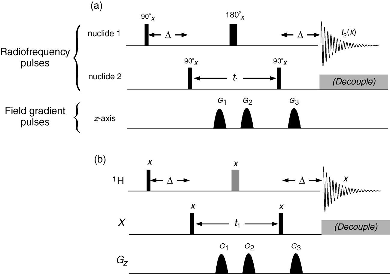
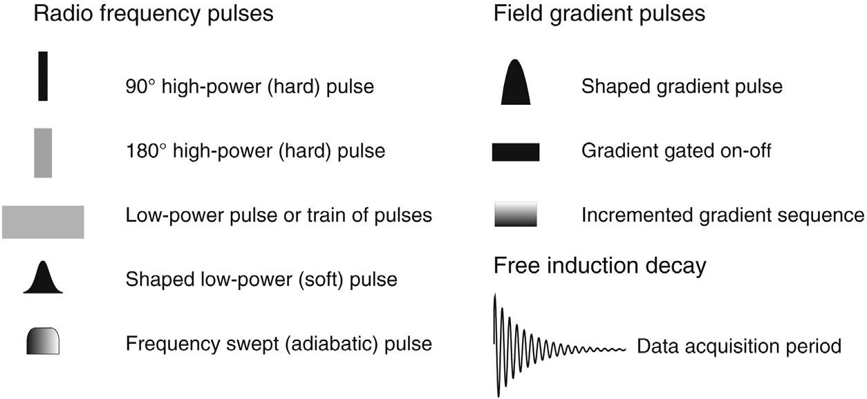
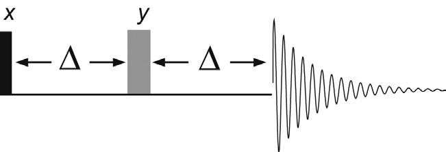
An example of a reasonably complex sequence is shown in Fig. 1.2 (a heteronuclear correlation experiment from the chapter Correlations Through the Chemical Bond II: Heteronuclear Shift Correlation) and illustrates most points of significance. Fig. 1.2a represents a more detailed account of the sequence, while Fig. 1.2b is the reduced equivalent used throughout the book for reasons of clarity. Radiofrequency (rf) pulses applied to each nuclide involved in the experiment are presented on separate rows running left to right, in the order in which they are applied. Most experiments nowadays involve protons, often combined with one (and sometimes two) other nuclides. This is most frequently carbon but need not be, so it is termed the X-nucleus. These rf pulses are most frequently applied as so-called 90 or 180 degree pulses (the significance of which is detailed in the following chapter), which are illustrated by a thin black bar and a thick grey bar respectively (Fig. 1.3). Pulses of other angles are marked with an appropriate Greek symbol that is described in the accompanying text. All rf pulses also have associated with them a particular phase, typically defined in units of 90 degrees (0, 90, 180, 270 degrees), and indicated above each pulse by x, y, –x or –y respectively. If no phase is defined the default will be x. Pulses that are effective over only a small frequency window and act only on a small number of resonances are differentiated as shaped rather than rectangular bars as this reflects the manner in which these are applied experimentally. These are the so-called selective or shaped pulses described in the chapter Experimental Methods. Pulses that sweep over very wide bandwidths are indicated by horizontal shading to reflect the frequency sweep employed, as also explained
FIGURE 1.2 Pulse sequence nomenclature. (a) Complete pulse sequence and (b) the reduced representation used throughout the remainder of the book.
FIGURE 1.3 A summary of the pulse sequence elements used throughout the book.
in the chapter Experimental Methods. Segments that make use of a long series of very many closely spaced pulses, such as the decoupling shown in Fig. 1.2, are shown as a solid grey box, with the bracket indicating the use of the decoupling sequence is optional. Below the row(s) of radiofrequency pulses are shown field gradient pulses ( Gz), whenever these are used, again drawn as shaped pulses where appropriate, and shown greyed when considered optional elements within a sequence.
The operation of very many NMR experiments is crucially dependent on the experiment being tuned to the value of specific coupling constants. This is achieved by defining certain delays within the sequence according to these values, these delays being indicated by the general symbol ∆. Other time periods within a sequence which are not tuned to J values but are chosen according to other criteria, such as spin recovery (relaxation) rates, are given the symbol τ. The symbols t1 and t2 are reserved for the time periods which ultimately correspond to the frequency axes f1 and f2 of 2D spectra, one of which (t2) will always correspond to the data acquisition period when the NMR response is actually detected. The acquisition period is illustrated by a simple decaying sine wave in all experiments to represent so-called free induction decay (FID). Again it should be stressed that although these sequences can have rather foreboding appearances, they are generally built up from much smaller and simpler segments that have well-defined and easily understood actions. A little perseverance can clarify what might at first seem a total enigma.
1.3 APPLYING MODERN NMR TECHNIQUES
The tremendous growth in available NMR pulse methods over the last three decades can be bewildering and may leave one wondering just where to start or how best to make use of these new developments. The answer to this is not straightforward since it depends so much on the chemistry undertaken, on the nature of the sample being handled and on the information required of it. It is also dependent on the amount of material and by the available instrumentation and its capabilities. The fact that NMR itself finds application in so many research areas means defined rules for experiment selection are largely intractable. A scheme that is suitable for tackling one type of problem may be wholly inappropriate for another. Nevertheless, it seems inappropriate that a book of this sort should contain no guidance on experiment selection other than the descriptions of the techniques in the following chapters. Here I attempt to broach this topic in rather general terms and present some loose guidelines to help weave a path through the maze of available techniques. Even so, only with a sound understanding of modern techniques can one truly be in a position to select the optimum experimental strategy for your molecule or system, and it is this understanding I hope to develop in the remaining chapters. The final chapter serves to illustrate application of the more common techniques to a single compound and also provides something of a guide to their likely use.
Most NMR investigations will begin with analysis of the proton spectrum of the sample of interest, with the usual analysis of chemical shifts, coupling constants and relative signal intensities, either manually or with the assistance of the various sophisticated computational databases now available. Beyond this, one encounters a plethora of available NMR methods to consider employing. The key to selecting appropriate experiments for the problem at hand is an appreciation of the type of information the principal NMR techniques can provide. Although there exist a huge number of pulse sequences, there are a relatively small number of what might be called core experiments, from which most others are derived by minor variation, of which only a rather small fraction ever find widespread use in the research laboratory. To begin, it is perhaps instructive to realise that the NMR methods presented in this book exploit four basic phenomena:
1. Through-bond interactions: scalar (J) spin coupling via bonding electrons.
2. Through-space interactions: the NOE mediated through dipole–dipole coupling and spin relaxation.
3. Chemical exchange: the physical exchange of one spin for another at a specific location.
4. Molecular self-diffusion: the translational movement of a molecule or complex.
When attempting to analyse the structure of a molecule and/or its behaviour in solution by NMR spectroscopy, one must therefore consider how to exploit these phenomena to gain the desired information, and from this select the appropriate technique(s). Thus, when building up the structure of a molecule one typically first searches for evidence of scalar coupling between nuclei as this can be used to indicate the location of chemical bonds. When the location of all bonding relationships within the molecule have been established, the gross structure of the molecule is defined. Spatial proximities between nuclei, and between protons in particular, can be used to define stereochemical relationships within a molecule and thus address questions of configuration and conformation. The unique feature of NMR spectroscopy, and the principal reason for its superiority over any other solution-state technique for structure elucidation, is its ability to define relationships between specific nuclei within a molecule or even between molecules. Such exquisite detail is generally obtained by correlating one nucleus with another by exploiting the above phenomena. Despite the enormous power of NMR, there are, in fact, rather few types of correlation available to the chemist to employ for structural and conformational analysis. The principal spin interactions and the main techniques used to map these, which are frequently 2D methods, are summarised
TABLE 1.2 The Principal Correlations or Interactions Established Through NMR Techniques
Proton J coupling typically over 2 or 3 bonds.
Relayed proton J couplings within a coupled spin system. Remote protons may be correlated provided there is a continuous coupling network in between them.
One-bond heteronuclear couplings with proton observation.
Long-range heteronuclear couplings with proton observation. Typically over 2 or 3 bonds when X = 13C.
COSY only used when X-spin natural abundance > 20%. Sensitivity problems when X has low natural abundance; can be improved with proton detection methods.
Through-space correlations. ROESY applicable to ‘mid-sized’ molecules with masses of ca. 1–2 kDa.
Interchange of spins at chemically distinct locations. Exchange must be slow on NMR timescale for separate resonances to be observed. Intermediate to fast exchange requires lineshape analysis.
Measurement of molecular self-diffusion using pulsed field gradient technology. Used often in studies of molecular associations.
The qualitative detection of ligand binding to a macromolecular receptor, most often a protein, and the quantitative determination of binding affinities.
in Table 1.2, further elaborated in the chapters that follow, and the use of the primary techniques illustrated in the chapter Structure Elucidation and Spectrum Assignment
The homonuclear correlation spectroscopy (COSY) experiment identifies those nuclei that share a J coupling, which, for protons, operate over two, three and, less frequently, four bonds. This information can therefore be used to indicate the presence of a bonding pathway. The correlation of protons that exist within the same coupled network or chain of spins, but do not themselves share a J coupling, can be made with the total correlation spectroscopy (TOCSY) experiment. This can be used to identify groups of nuclei that sit within the same isolated spin system, such as the amino acid residue of a peptide or the sugar ring of an oligosaccharide. One-bond heteronuclear correlation methods—heteronuclear single quantum correlation (HSQC) or heteronuclear multiple quantum correlation (HMQC)—identify the heteroatoms to which the protons are directly attached and can, for example, provide carbon assignments from previously established proton assignments. Proton chemical shifts can also be dispersed according to the shift of the attached heteroatom, so aiding the assignment of the proton spectrum itself. Long-range heteronuclear correlations over typically two or three-bonds—heteronuclear multiple bond correlation (HMBC)—provide a wealth of information on the skeleton of the molecule and can be used to infer the location of carbon–carbon or carbon–heteroatom bonds. These correlations can be particularly valuable when sufficient proton–proton correlations are absent. Techniques based on the INADEQUATE (incredible natural abundance double quantum transfer) experiment identify connectivity between similar nuclei of low natural abundance. These can therefore correlate directly connected carbon centres, but as they rely on the presence of neighbouring carbon-13 nuclei they suffer from appallingly low sensitivity and thus find limited use. Modern variants that use proton detection, termed ADEQUATE (adequate sensitivity double quantum spectroscopy), have greatly improved performance but are still less used than the above heteronuclear correlation techniques. Measurements based on the NOE are most often applied after the gross structure is defined, and NMR assignments established, to define the 3D stereochemistry of a molecule since these effects map through-space proximity between nuclei. It can also provide insights into the conformational folding of larger structures and on direct intermolecular interactions. The vast majority of these experiments investigate proton–proton NOEs, although heteronuclear NOEs involving a proton and a heteroatom have been applied successfully. Similar techniques to those used in the observation of NOEs can also be employed to correlate nuclei involved in chemical exchange processes that are slow on the NMR timescale and so give rise to distinct resonances for each exchanging species or site. Finally, methods for the quantification of molecular self-diffusion provide information on the nature and extent of molecular associations and provide a complimentary view of solution behaviour. They may also be used to separate the spectra of species with differing mobilities and have potential application in the characterisation of mixtures.
The greatest use of NMR in the chemical research laboratory is in the routine characterisation of synthetic starting materials, intermediates and final products. In these circumstances it is often not so much full structure elucidation that is required, rather it is structure confirmation or verification since the synthetic reagents are known, which naturally limit what the products may be, and because the synthetic target is usually defined. Routine analysis of this sort typically follows a general procedure similar to that summarised in Table 1.3, which is supplemented with data from other analytical techniques, most notably mass spectrometry and infrared spectroscopy. Execution of many of the experiments in Table 1.3 benefits nowadays from the incorporation of pulsed field gradients to speed data collection and to provide spectra of higher quality. Nowadays, the collection of a 2D proton-detected 1H–13C shift correlation experiment such as HSQC requires significantly less time than the 1D carbon spectrum of the same sample, providing both carbon shift data (of protonated centres) and correlation information. This can be a far more powerful tool for routine structure confirmation than the 1D carbon experiment alone. In addition, editing can be introduced to the 2D experiment to differentiate methine from methylene correlations, for example providing yet more data in a single experiment and in less time. Even greater gains can be made in the indirect observation of heteronuclides of still lower intrinsic sensitivity, for example nitrogen-15, and when considering the observation of low-abundance nuclides it is sensible to first consider adopting a proton-detected method for this. The structure confirmation process can also be enhanced through measured use of spectrum prediction tools that are now widely available. Generation of a calculated spectrum from a proposed structure can provide useful guidance when considering the validity of the structure and a number of computational packages are now available that predict at least 13C and 1H spectra, but also the more common nuclides including 19F, 31P and 15N in some cases. Even when dealing with unknown materials or with molecules of high structural complexity, the general scheme of Table 1.3 still represents an appropriate general protocol to follow, as demonstrated in the chapter Structure Elucidation and Spectrum Assignment. In such cases, the basic experiments of this table are still likely to be employed, but may require data to be collected under a variety of experimental conditions (solvent, temperature, pH etc.) and/or may require additional support from other methods or extended versions of these techniques before a complete picture emerges. This book aims to explain the primary NMR techniques and some of their more useful variants, and to describe their practical implementation, so that the research chemist may realise the full potential that modern NMR spectroscopy has to offer.
TABLE 1.3
A
Typical Protocol for Routine Structure Confirmation of Synthetic Organic Materials
Information from chemical shifts, coupling constants, integrals
Identify J-coupling relationships between protons
Carbon count and multiplicity determination (C, CH, CH2, CH3). Can often be avoided by using proton-detected heteronuclear 2D experiments.
Chemical shifts and homonuclear/heteronuclear coupling constants.
Carbon assignments transposed from proton assignments. Proton spectrum dispersed by 13C shifts. Carbon multiplicities from edited HSQC (faster than above 1D approach).
Correlations identified over two and three bonds. Correlations established across heteroatoms (eg N and O). Fragments of structure pieced together.
Stereochemical analysis: configuration and conformation.
Not all these steps may be necessary, and the direct observation of a heteronuclide, such as carbon or nitrogen, can often be replaced through its indirect observation with more sensitive proton-detected heteronuclear shift correlation techniques.
[16] Zerbe O. BioNMR in drug research, vol. 16. Weinheim: Wiley-VCH; 2003
[17] Roberts GCK, Lian L-Y. Protein NMR spectroscopy: practical techniques and applications. Weinheim: Wiley; 2011
[18] Cavanagh J, Fairbrother WJ, Palmer AG, Skelton NJ, Rance M. Protein NMR spectroscopy: principles and practice. 2nd ed. San Diego: Academic Press (Elsevier); 2006
Chapter 2
Introducing High-Resolution NMR
Chapter Outline
2.1
2.4.1
2.4.3
2.4.4
For anyone wishing to gain a greater understanding of modern nuclear magnetic resonance (NMR) techniques together with an appreciation of the information they can provide and hence their potential applications, it is necessary to develop an understanding of some elementary principles. These, if you like, provide the foundations from which the descriptions in subsequent chapters are developed and many of the fundamental topics presented in this introductory chapter will be referred to throughout the remainder of the text. In keeping with the style of the book, all concepts are presented in a pictorial manner and avoid the more mathematical descriptions of NMR. Following a reminder of the phenomenon of nuclear spin, the Bloch vector model of NMR is introduced. This presents a convenient picture of how spins behave in an NMR experiment and provides the basic tools with which most experiments will be described. It is used in the description of spin relaxation processes, after which responsible relaxation mechanisms are described together with methods for measuring relaxation rates. Finally, the chapter considers the appearance of NMR spectra when influenced by the internal dynamics of chemical structures, and describes techniques for measuring the rates of chemical exchange processes.
2.1 NUCLEAR SPIN AND RESONANCE
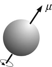
The nuclei of all atoms may be characterised by a nuclear spin quantum number I , which may have values greater than or equal to zero and which are multiples of ½. Those with I = 0 possess no nuclear spin and therefore cannot exhibit NMR, so are termed ‘NMR silent’. Unfortunately, from the organic chemist’s point of view, the nucleus likely to be of most interest, carbon-12, has zero spin, as do all nuclei with atomic mass and atomic number that are both even. However, the vast majority of chemical elements have at least one nuclide that does possess nuclear spin which is, in principle at least, observable by NMR ( Table 2.1 ) and as a consolation the proton is a high-abundance NMR-active isotope. The property of nuclear spin is fundamental to the NMR phenomenon. The spinning nuclei possess angular momentum P and, of course, charge and the motion of this charge gives rise to an associated magnetic moment m ( Fig. 2.1 ) such that:
TABLE 2.1 Properties of Selected Spin-½ Nuclei
Frequencies are given for a 400-MHz spectrometer (9.4-T magnet) and sensitivities are given relative to proton observation and include terms for both intrinsic sensitivity of the nucleus and its natural abundance. aAssuming 100% 3H labelling. The properties of quadrupolar nuclei are given in Table 2.3
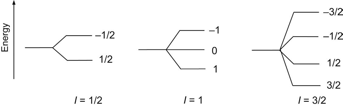
where the term g is the magnetogyric ratio which is constant for any given nuclide and may be viewed as a measure of how ‘strongly magnetic’ a particular nuclide is. The term gyromagnetic ratio is also in widespread use for g, although this does not conform to IUPAC recommendations [1–3]. Both angular momentum and the magnetic moment are vector quantities; that is, they have both magnitude and direction. When placed in an external, static magnetic field (denoted B0, strictly the magnetic flux density) the microscopic magnetic moments align themselves relative to the field in a discrete number of orientations because the energy states involved are quantised. For a spin of magnetic quantum number I there exist 2I + 1 possible spin states, so for a spin-½ nucleus such as the proton, there are two possible states denoted +½ and –½, while for I = 1, for example deuterium, the states are +1, 0 and –1 (Fig. 2.2) and so on. For the spin-½ nucleus, the two states correspond to the popular picture of a nucleus taking up two possible orientations with respect to the static field, either parallel (the a state) or antiparallel (the b state), the former being of lower energy. The effect of the static field on the magnetic moment can be described in terms of classical mechanics, with the field imposing a torque on the moment, which therefore
FIGURE 2.2 Nuclear spin states. Nuclei with a magnetic quantum I may take up 2I + 1 possible orientations relative to the applied static magnetic field B0 For spin-½ nuclei, this gives the familiar picture of the nucleus behaving as a microscopic bar magnet having two possible orientations, a and b
FIGURE 2.1 Nuclear magnetic moments. A nucleus carries charge and when spinning possesses a magnetic moment m.
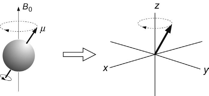
FIGURE 2.3 Larmor precession. A static magnetic field applied to the nucleus causes it to precess at a rate dependent on the field strength and the magnetogyric ratio of the spin. The field is conventionally applied along the z-axis of a Cartesian co-ordinate frame and the motion of the nucleus represented as a vector moving on the surface of a cone.
traces a circular path about the applied field (Fig. 2.3). This motion is referred to as precession, or more specifically Larmor precession in this context. It is analogous to the familiar motion of a gyroscope in the Earth’s gravitational field, in which the gyroscope spins about its own axis, and this axis in turn precesses about the direction of the field. The rate of precession as defined by the angular velocity (w rad s–1 or ν Hz) is:
(The symbol g in place of g/2π will occur frequently throughout the text when representing frequencies in hertz.) This is known as the Larmor frequency of the nucleus. The direction of motion is determined by the sign of g and may be clockwise or anticlockwise, but is always the same for any given nuclide. NMR occurs when the nucleus changes its spin state, driven by the absorption of a quantum of energy. This energy is applied as electromagnetic radiation, whose frequency must match that of Larmor precession for the resonance condition to be satisfied, with the energy involved being given by:
where h is Planck’s constant. In other words, the resonant frequency of a spin is simply its Larmor frequency. Modern high-resolution NMR spectrometers currently (2015) employ field strengths up to 23.5 T (tesla) which, for protons, correspond to resonant frequencies up to 1000 MHz that fall within the radiofrequency region of the electromagnetic spectrum. For other nuclei at similar field strengths, resonant frequencies will differ from those of protons (due to the dependence of ν on g) but it is common practice to refer to a spectrometer’s operating frequency in terms of the resonant frequencies of protons. Thus, one may refer to using a ‘400-MHz spectrometer’, although this would equally operate at 100-MHz for carbon-13 since gH/gC ≈ 4. It is also universal practice to define the direction of the static magnetic field as being along the z-axis of a set of Cartesian coordinates, so that a single precessing spin-½ nucleus will have a component of its magnetic moment along the z-axis (the longitudinal component) and an orthogonal component in the x–y plane (the transverse component) (Fig. 2.3).
Now consider a collection of similar spin-½ nuclei in the applied static field. As stated, the orientation parallel to the applied field a has slightly lower energy than the anti-parallel orientation b, so at equilibrium there will be an excess of nuclei in the a state as defined by the Boltzmann distribution:
(2.4)
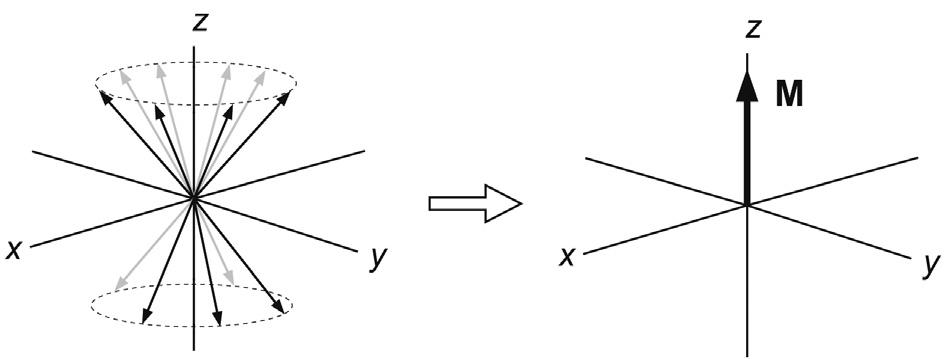
where Na,b represents the number of nuclei in the spin orientation, kB the Boltzmann constant and T the temperature. The differences between spin energy levels are rather small so the corresponding population differences are similarly small and only about one part in 104 at the highest available field strengths. This is why NMR is so very insensitive relative to other techniques such as IR and UV, where ground-state and excited-state energy differences are substantially greater. The tiny population excess of nuclear spins can be represented as a collection of spins distributed randomly about the precessional cone and parallel to the z-axis. These give rise to a resultant bulk magnetisation vector M along this axis (Fig. 2.4). It is important to realise that this z-magnetisation arises because of population differences between the possible spin states, a point we return to in Section 2.2. Since there is nothing to define a preferred orientation for the spins in the transverse direction, there exists a random distribution of individual magnetic moments about the cone and hence there is no net magnetisation in the transverse (x–y) plane. Thus, we can reduce our picture of many similar magnetic moments to one of a single bulk magnetisation vector M that behaves according to the rules of classical mechanics. This simplified picture
FIGURE 2.4 Bulk magnetisation. In the vector model of NMR many like spins are represented by a bulk magnetisation vector. At equilibrium the excess of spins in the a state places this parallel to the +z-axis.
is referred to as the Bloch vector model (after the pioneering spectroscopist Felix Bloch), or more generally as the vector model of NMR.
2.2 THE VECTOR MODEL OF NMR
Having developed the basic model for a collection of nuclear spins, we can now describe the behaviour of these spins in pulsed NMR experiments. There are essentially two parts to be considered: firstly the application of the radiofrequency (rf) pulse(s) and, secondly the events that occur following this. The essential requirement to induce transitions between energy levels, that is to cause resonance to occur, is the application of a time-dependent magnetic field oscillating at the Larmor frequency of the spin. This field is provided by the magnetic component of the applied rf, which is designated the B1 field to distinguish it from the static B0 field. This rf is transmitted via a coil surrounding the sample, the geometry of which is such that the B1 field exists in the transverse plane, perpendicular to the static field. In trying to consider how this oscillating field operates on the bulk magnetisation vector, one is faced with a mind-boggling task involving simultaneous rotating fields and precessing vectors. To help visualise these events it proves convenient to employ a simplified formalism, known as the rotating frame of reference, as opposed to the so-called laboratory frame of reference described thus far.
2.2.1 The Rotating Frame of Reference
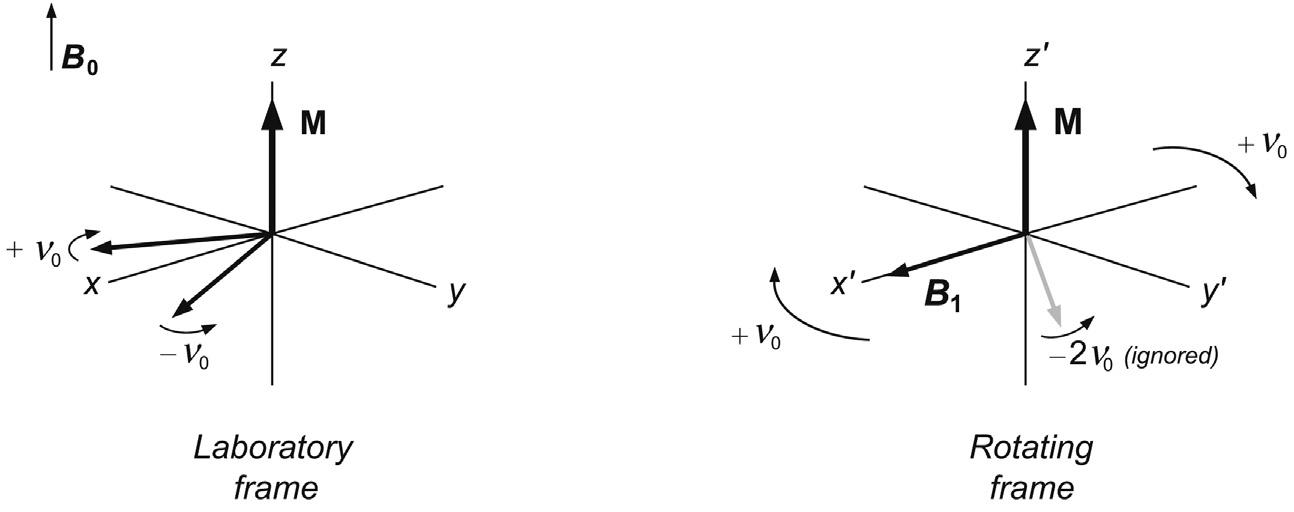
To aid the visualisation of processes occurring during an NMR experiment a number of simple conceptual changes are employed. Firstly, the oscillating B1 field is considered to be composed of two counter-rotating magnetic vectors in the x–y plane, the resultant of which corresponds exactly to the applied oscillating field (Fig. 2.5). It is now possible to simplify things considerably by eliminating one of these and simultaneously freezing the motion of the other by picturing events in the rotating frame of reference (Fig. 2.6). In this, the set of x, y, z co-ordinates are viewed as rotating along with the nuclear precession, in the same sense and at the same rate. Since the frequency of oscillation of the rf field exactly matches that of nuclear precession (which it must for the magnetic resonance condition to be satisfied), the rotation of one of the rf vectors is now static in the rotating frame whereas the other is moving at twice the frequency in the opposite direction. This latter vector is far from resonance and is simply ignored. Similarly, the precessional motion of the spins has been frozen as these are moving with the same angular velocity as the rf vector and hence the co-ordinate frame. Since this precessional motion was induced by the static magnetic field B0, this is also no longer present in the rotating frame representation.
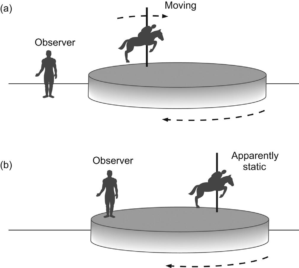
The concept of the rotating frame may be better pictured with the following analogy. Suppose you are at a fairground and are standing watching a child going round on the carousel. You see the child move towards you then away from you as the carousel turns, and are thus aware of the circular path the child follows. This corresponds to observing events from the so-called laboratory frame of reference (Fig. 2.7a). Now imagine what you see if you step onto the carousel as it turns. You are now travelling with the same angular velocity and in the same sense as the child so the child’s motion is no longer
FIGURE 2.5 The B1 field. The rf pulse provides an oscillating magnetic field along one axis (here the x-axis) which is equivalent to two counter-rotating vectors in the transverse plane.
FIGURE 2.6 Laboratory and rotating frame representations. In the laboratory frame the coordinate system is viewed as being static, whereas in the rotating frame it rotates at a rate equal to the applied rf frequency ν0. In this representation the motion of one component of the applied rf is frozen whereas the other is far from the resonance condition and may be ignored. This provides a simplified model for the description of pulsed NMR experiments.
2.7 Frames of reference. A fairground carousel can be viewed from (a) the laboratory or (b) the rotating frame of reference.
apparent. The child’s precession has been frozen from your point of view and you are now observing events in the rotating frame of reference (Fig. 2.7b). Obviously the child is still moving in the ‘real’ world but your perception of events has been greatly simplified. Likewise, this transposition simplifies our picture of events in an NMR experiment.
Strictly one should use a different co-ordinate labelling scheme for the laboratory and the rotating frames, such as x, y, z and x', y' and z', respectively, as in Fig. 2.6. However, since we shall be dealing almost exclusively with a rotating frame description of events, the simpler x, y, z notations will be used throughout the remainder of the book, and explicit indication provided where the laboratory frame of reference is used.
2.2.2 Pulses
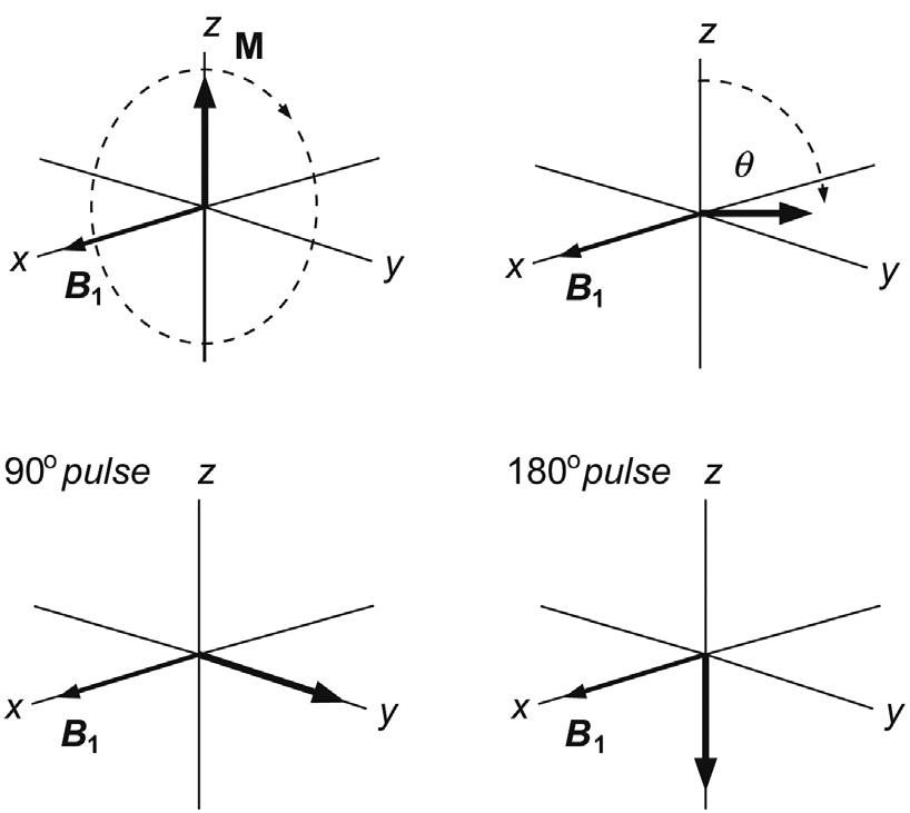
We are now in a position to visualise the effect of applying an rf pulse to the sample. The ‘pulse’ simply consists of turning on rf irradiation of a defined amplitude for a time period tp, and then switching it off. As in the case of the static magnetic field, the rf electromagnetic field imposes a torque on the bulk magnetisation vector in a direction perpendicular to the direction of the B1 field (the ‘motor rule’) that rotates the vector from the z-axis towards the x–y plane (Fig. 2.8). Thus, applying the rf field along the x-axis will drive the vector towards the y-axis. [Strictly speaking, the sense of rotation is positive about the applied B1 field so that the vector will be driven towards the –y-axis. For clarity of presentation, the vector will always been shown as coming out of the page towards the +y-axis for a pulse applied along the +x-axis.] The rate at which the vector moves is proportional to the strength of the rf field ( γ B1), and so the angle u through which the vector
FIGURE
FIGURE 2.8 The radiofrequency (rf) pulse. An rf pulse applies a torque to the bulk magnetisation vector and drives it towards the x–y plane from equilibrium. u is the pulse tip or flip angle which is most frequently 90 or 180 degrees.
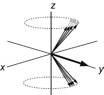
FIGURE 2.9 Phase coherence. Following a 90 degree pulse, individual spin vectors bunch along the y-axis and are said to possess phase coherence.
turns, colloquially known as the pulse flip or tip angle (but more formally as the nutation angle), will be dependent on the amplitude and duration of the pulse:
θγ = Bt 360degrees p 1 (2.5)
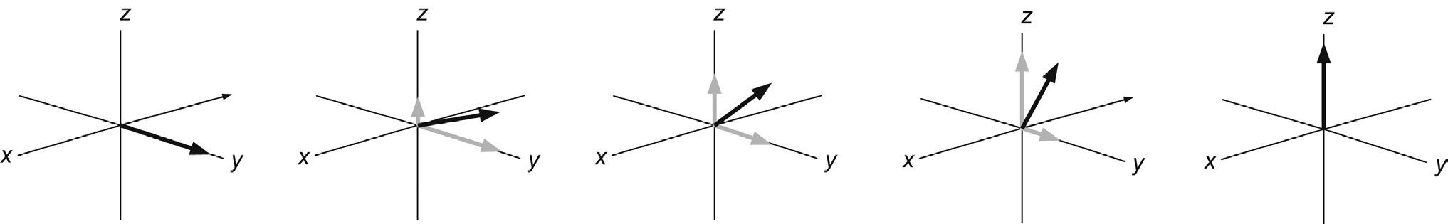
If the rf was turned off just as the vector reached the y-axis, this would represent a 90 degree pulse, if it reached the –z-axis, it would be a 180 degree pulse, and so on. Returning to consider the individual magnetic moments that make up the bulk magnetisation vector for a moment, we see that the 90 degrees pulse corresponds to equalising the populations of the a and b states, as there is now no net z-magnetisation. However, there is net magnetisation in the x–y plane, resulting from ‘bunching’ of the individual magnetisation vectors caused by application of the rf pulse. The spins are said to possess phase coherence at this point, forced upon them by the rf pulse (Fig. 2.9). Note that this equalising of populations is not the same as the saturation of a resonance, a condition that will be encountered in a variety of circumstances in this book. Saturation corresponds again to equal spin populations but with the phases of the individual spins distributed randomly about the transverse plane such that there exists no net transverse magnetisation and thus no observable signal. In other words, under conditions of saturation the spins lack phase coherence. The 180 degree pulse inverts the populations of the spin states, since there must now exist more spins in the b than in the a orientation to place the bulk vector anti-parallel to the static field. Only magnetisation in the x–y plane is ultimately able to induce a signal in the detection coil (see later in the chapter) so that the 90 and 270 degrees pulse will produce maximum signal intensity, but the 180 and 360 degrees pulse will produce none (this provides a useful means of ‘calibrating’ the pulses, as in the following chapter). The vast majority of the multipulse experiments described in this book, and indeed throughout NMR, use only 90 and 180 degrees pulses.
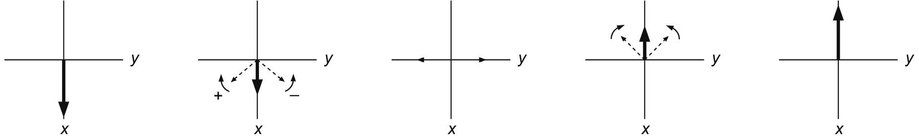
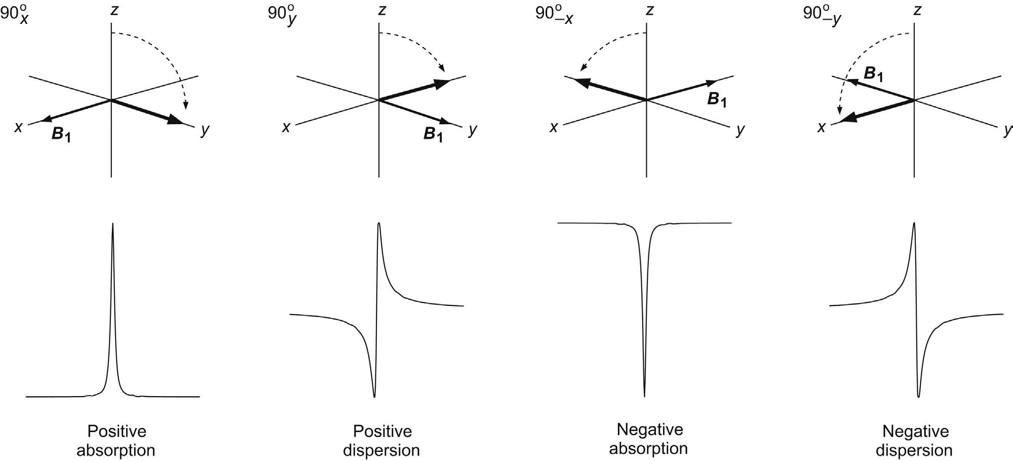
The example above made use of a 90x pulse; that is a 90 degree pulse in which the B1 field was applied along the x-axis. It is however possible to apply the pulse with arbitrary phase, say, along any of the axes x, y, –x or –y as required, which translates to a different starting phase of the excited magnetisation vector. The spectra provided by these pulses show resonances whose phases similarly differ by 90 degrees. The detection system of the spectrometer designates one axis to represent the positive absorption signal (defined by a receiver reference phase, Section 3.2.2) meaning only magnetisation initially aligned with this axis will produce a pure absorption-mode resonance. Magnetisation that differs from this by +90 degrees is said to represent the pure dispersion-mode signal, that which differs by 180 degree is the negative absorption response and so on (Fig. 2.10). Magnetisation vectors initially between these positions result in resonances displaying a mixture of absorption and dispersion behaviour. For clarity and optimum resolution, all resonance peaks are displayed in the favoured absorption mode whenever possible (which is achieved through a process known as phase correction). Note that in all cases the detected signals are those emitted from the nuclei as described later, and a negative phase signal does not imply a change from emission to absorption of radiation (absorption corresponds to initial excitation of the spins).
The idea of applying a sequence of pulses of different phase angles is of central importance to all NMR experiments. The process of repeating a multipulse experiment with different pulse phases and combining the collected data in an appropriate manner is termed phase cycling, and is one of the most widely used procedures for selecting the signals of
FIGURE 2.10 Excitation with pulses of varying rf phase. The differing initial positions of the excited vectors produce NMR resonances with similarly altered phases (here the y axis is arbitrarily defined as representing the positive absorption display).
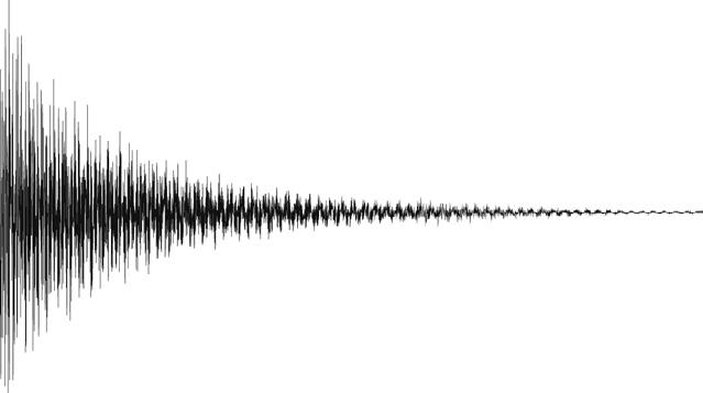
FIGURE 2.11 The NMR response detected: an FID. The signal fades as the nuclear spins relax back towards their equilibrium state.
interest in an NMR experiment and rejecting those that are not required. We shall encounter this concept further in the chapter Practical Aspects of High-Resolution NMR, and indeed throughout the book.
Now consider what happens immediately after application of, for example a 90°x pulse. We already know that in the rotating frame the precession of spins is effectively frozen because the B1 frequency ν0 and hence the rotating frame frequency exactly match the spin Larmor frequency. Thus, the bulk magnetisation vector simply remains static along the +y-axis. However, if we step back from our convenient ‘fiction’ and return to consider events in the laboratory frame, we see that the vector starts to precess about the z-axis at its Larmor frequency. This rotating magnetisation vector will produce a weak oscillating voltage in the coil surrounding the sample, in much the same way that the rotating magnet in a classic bicycle dynamo induces a voltage in the coils that surround it. These are the electrical signals we wish to detect and it is these that ultimately produce the observed NMR signal. However, magnetisation in the x–y plane corresponds to deviation from equilibrium spin populations and, just like any other chemical system that is perturbed from its equilibrium state, the system will adjust to re-establish this condition, and so the transverse vector will gradually disappear and simultaneously grow along the z-axis. This return to equilibrium is referred to as relaxation, and it causes the NMR signal to decay with time, producing the observed free induction decay (FID) (Fig. 2.11). The process of relaxation has wide-ranging implications for the practice of NMR and this important area is also addressed in this introductory chapter.
2.2.3 Chemical Shifts and Couplings
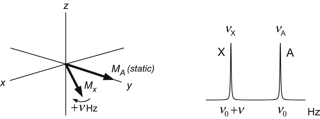
So far we have only considered the rotating frame representation of a collection of like spins, involving a single vector which is stationary in the rotating frame since the reference frequency ν0 exactly matches the Larmor frequency of the spins (the rf is said to be on-resonance for these spins). Now consider a sample containing two groups of chemically distinct but uncoupled spins A and X with chemical shifts of νA and νX, respectively, which differ by ν Hz. Following
FIGURE 2.12 Chemical shifts in the rotating frame. Vectors evolve according to their offsets from the reference (transmitter) frequency ν0. Here this is on-resonance for spins A (ν0 = νA) while spins X move ahead at a rate of +ν Hz (= νX – ν0).
excitation with a single 90°x pulse, both vectors start in the x–y plane along the y-axis of the rotating frame. Choosing the reference frequency to be on-resonance for the A spins (ν0 = νA) means these remain along the y-axis as before (ignoring the effects of relaxation for the present). If the X spins have a greater chemical shift than A (νX > νA) then the X vector will be moving faster than the rotating frame reference frequency by the difference ν Hz so will move ahead of A (Fig. 2.12). Conversely, if νX < νA it will be moving more slowly and will lag behind. Three sets of uncoupled spins can be represented by three rotating vectors and so on, such that differences in chemical shifts between spins are simply represented by vectors precessing at different rates in the rotating frame, according to their offsets from the reference frequency ν0. By using the rotating frame to represent these events we need only consider chemical shift differences between the spins of interest, which will be in the kilohertz range, rather than the absolute frequencies, which are of the order of many megahertz. As we shall discover in Section 3.2, this is exactly analogous to the operation of the detection system of an NMR spectrometer, in which a reference frequency is subtracted from the acquired data to produce signals in the kHz region suitable for digitisation. Thus, the ‘trick’ of using the rotating frame of reference in fact equates directly to a real physical process within the instrument.
When considering the effects of scalar coupling on-resonance it is convenient to remove the effects of chemical shift altogether by choosing the reference frequency of the rotating frame to be the chemical shift of the multiplet of interest. This again helps clarify our perception of events by simplifying rotation of the vectors in the picture. In the case of a doublet, the two lines are represented by two vectors precessing at +J/2 and –J/2 Hz, while for a triplet, the central line remains static and the outer two move at +J and –J Hz (Fig. 2.13). In many NMR experiments it is desirable to control the orientation of multiplet vectors with respect to one another, and, as we shall see, a particularly important relationship is when two vectors are anti-phase to one another, that is sitting in opposite directions. This can be achieved simply by choosing an appropriate delay period in which the vectors evolve, which is 1/2J for a doublet but 1/4J for the triplet.
2.2.4 Spin-Echoes
Having seen how to represent chemical shifts and J couplings with the vector model, we are now in a position to see how we can manipulate the effects of these properties in simple multi-pulse experiments. The idea here is to provide a simple introduction to using the vector model to understand what is happening during a pulse sequence. In many experiments, there exist time delays in which magnetisation is simply allowed to precess under the influence of chemical shifts and couplings, usually with the goal of producing a defined state of magnetisation before further pulses are applied or data are acquired. To illustrate these points, we consider one of the fundamental building blocks of numerous NMR experiments: the spin echo.
Consider first two groups of chemically distinct protons A and X that share a mutual coupling JAX, which will be subject to the simple two-pulse sequence in Fig. 2.14. For simplicity we shall consider the effect of chemical shifts and couplings separately, starting with chemical shifts and again assuming the reference frequency to be that of the A spins (Fig. 2.15). The initial 90°x creates transverse A and X magnetisation, after which the X vector precesses during the first time interval ∆ The following 180°y pulse (note this is now along the y-axis) rotates the X magnetisation through 180 degrees about the y-axis, and so places it back in the x–y plane, but now lagging behind the A vector. A-spin magnetisation remains along the y-axis so is invariant to this pulse. During the second time period ∆, the X magnetisation will precess through the same angle as in the first period and at the end of the sequence finishes where it began and at the same position as the A vector. Thus, after the time period 2∆ no phase difference has accrued between the A and X vectors despite their different shifts, and it were as if the A and X spins had the same chemical shift throughout the 2∆ period. We say the spin-echo has refocused the chemical shifts, the dephasing and rephasing stages giving rise to the echo terminology.
2.13 Scalar couplings in the rotating frame. Multiplet components evolve according to their coupling constants. The vectors have an antiphase disposition after an evolution period of 1/2J and 1/4J s for doublets and triplets, respectively.
sequence.
Consider now the effect on the coupling between the two spins with reference to the multiplet of spin A, safe in the knowledge that we can ignore the effects of chemical shifts. Again, during the first period ∆ the doublet components will move in opposite directions, and then have their positions interchanged by application of the 180°y pulse. At this point it would be obvious to assume that the two halves of the doublets would simply refocus as in the case of the chemical shift differences above, but we have to consider the effect of the 180 degrees pulse on the J-coupled partner also; in other words, the effect on the X spins. To appreciate what is happening, we need to remind ourselves of what it is that gives rise to two halves of a doublet. These result from spin A being coupled to its partner X, which can have one of two orientations (a or b) with respect to the magnetic field. When spin X has one orientation, spin A will resonate as the high-frequency half of its
FIGURE
FIGURE 2.14 The basic spin-echo pulse
FIGURE 2.15 Chemical shift evolution is refocused with the spin-echo sequence.
FIGURE 2.16 The influence of spin-echoes on scalar coupling as illustrated for two coupled spins A and X. (a) A homonuclear spin echo (in which both spins experience a 180-degree pulse) allows the coupling to evolve throughout the sequence. (b) A heteronuclear spin echo (in which only one spin experiences a 180-degree pulse) causes the coupling to refocus. If both heteronuclear spins experience 180-degree pulses, the heteronuclear coupling evolves as in (a) (see text).
doublet, while with X in the other, A will resonate as the low-frequency half. As there are approximately the same number of X spins in the a and b orientations, the two halves of the A doublet will be of equal intensity (obviously there are not exactly equal numbers of a and b X spins, otherwise there would be no NMR signal to observe, but the difference is so small as to be negligible for these arguments). The effect of applying the 180 degrees pulse on the X spins is to invert the relative orientations, so that any A spin that was coupled to Xa is now coupled to Xb, and vice versa. This means the faster moving vector now becomes the slower and vice versa, the overall result being represented in Fig. 2.16a. The two halves of the doublet therefore continue to dephase, so that by the end of the 2∆ period, the J coupling, in contrast to the chemical shifts, have continued to evolve so that homonuclear couplings are not refocused by a spin-echo. The reason for adding the term homonuclear to the previous statement is because it does not necessarily apply to the case of heteronuclear spinechoes, that is when we are dealing with two different nuclides, such as 1H and 13C. This is because in a heteronuclear system one may choose to apply the 180 degree pulse on only one channel, thus only one of the two nuclides will experience this pulse and refocusing of the heteronuclear coupling will occur in this case (Fig. 2.16b). If two simultaneous 180 degree pulses are applied to both nuclei via two different frequency sources, continued defocusing of the heteronuclear coupling occurs exactly as for the homonuclear spin-echo above.
The use of the 180°y pulse instead of a 180°x pulse in the above sequences was employed to provide a more convenient picture of events, yet it is important to realise that the refocusing effects on chemical shift and couplings described earlier would also have occurred with a 180°x pulse except that the refocused vectors would now lie along the –y-axis instead of the +y-axis. One further feature of the spin-echo sequence is that it will also refocus the deleterious effects that arise from inhomogeneities in the static magnetic field, as these may be viewed as just another contribution to chemical shift differences throughout the sample. The importance of the spin echo in modern NMR techniques can hardly be overemphasised. It allows experiments to be performed without having to worry about chemical shift differences within a sample and the complications these may introduce (eg phase differences). This then allows us to manipulate spins according to their couplings with neighbours and it is these interactions that are exploited to the full in many of the modern NMR techniques described later.
2.3 TIME AND FREQUENCY DOMAINS
It was shown in the previous section that the emitted rf signal from excited nuclear spins (the FID) is detected as a timedependent oscillating voltage which steadily decays as a result of spin relaxation. In this form the data are of little use to us because they are a time domain representation of the nuclear precession frequencies within the sample. What we actually want is a display of the frequency components that make up the FID as it is these we relate to transition energies and ultimately chemical environments. In other words, we need to transfer our time domain data into the frequency domain
The time and frequency domains are related by a simple function, one being the inverse of the other (Fig. 2.17). The complicating factor is that a genuine FID is usually composed of potentially hundreds of components of differing frequencies
and amplitude, in addition to noise and other possible artefacts, and in such cases the extraction of frequencies by direct inspection is impossible. By far the most widely used method to produce the frequency domain spectrum is the mathematical procedure of Fourier transformation, which has the general form:
where f(w) and f(t) represent the frequency and time domain data, respectively. In the very early days of pulse–Fourier transform (FT) NMR the transform was often the rate-limiting step in producing a spectrum, although with today’s computers and the use of a fast FT procedure (the Cooley–Tukey algorithm) the time requirements are of little consequence. Fig. 2.18 demonstrates this procedure for very simple spectra. Clearly, even for these rather simple spectra of only a few
FIGURE 2.17 Time and frequency domains share a simple inverse relationship.
FIGURE 2.18 Fourier transformation of time domain FIDs produces the corresponding frequency domain spectra.
lines the corresponding FID rapidly becomes too complex for direct interpretation, whereas this is impossible for a genuine FID of any complexity (see Fig. 2.11).
The details of the Fourier transform itself are usually of little consequence to anyone using NMR, although there is one notable feature to be aware of. The term eiwt can equally be written coswt + i sinwt and in this form it is apparent that the transformation actually results in two frequency domain spectra that differ only in their signal phases. The two are cosine and sine functions so are 90 degrees out of phase relative to one another and are termed the ‘real’ and ‘imaginary’ parts of the spectrum (because the function contains complex numbers). Generally, we are presented with only the ‘real’ part of the data (although the ‘imaginary’ part can usually be displayed) and with appropriate phase adjustment we choose this to contain the desired pure absorption-mode data and the imaginary part to contain the dispersion-mode representation. The significance of this phase relationship will be pursued in the chapters Practical Aspects of High-Resolution NMR and Introducing Two-Dimensional and Pulsed Field Gradient NMR
2.4 SPIN RELAXATION
The action of an rf pulse on a sample at thermal equilibrium perturbs the nuclear spins from this restful state. Following this perturbation, one would intuitively expect the system to re-establish the equilibrium condition, and lose the excess energy imparted into the system by the applied pulse. A number of questions then arise: Where does this energy go, how does it get there (or in other words what mechanisms are in place to transfer the energy), and how long does all this take? While some appreciation of all these points is desirable, it is the last of the three that has greatest bearing on the day-to-day practice of NMR. The lifetimes of excited nuclear spins are extremely long when compared with, say, the excited electronic states of optical spectroscopy. These may be a few seconds or even minutes for nuclear spins as opposed to less than a picosecond for electrons, a consequence of the low transition energies associated with nuclear resonance. These extended lifetimes are crucial to the success of NMR spectroscopy as an analytical tool in chemistry. Not only do these mean that resonance peaks are rather narrow relative to those of rotational, vibrational or electronic transitions (as a consequence of the Heisenberg Uncertainty principle), but it also provides time to manipulate the spin systems after their initial excitation, performing a variety of spin gymnastics and so modifying the information available in the resulting spectra. This is the world of multipulse NMR experiments, into which we shall enter shortly, and knowledge of relaxation rates has considerable bearing on the design of these experiments, on how they should be implemented and on the choice of experimental parameters for optimum results. Even in the simplest possible case of a single-pulse experiment, relaxation rates influence both achievable resolution and sensitivity (as mentioned in the opening chapter, the earliest attempts to observe the NMR phenomenon probably failed because of a lack of understanding at that time of the spin relaxation properties of the samples used).
The relaxation rates of nuclear spins can also be related to aspects of molecular structure and behaviour in favourable circumstances; in particular, internal molecular motions. It is true to say however that the relationship between relaxation rates and structural features are not as well defined as those of the chemical shift and spin–spin coupling constants, and are not used on a routine basis. The problem of reliable interpretation of relaxation data arises largely from the numerous extraneous effects that influence experimental results, meaning empirical correlations for using such data are not generally available and this aspect of NMR will not be further pursued.
Immediately after pulse excitation of nuclear spins the bulk magnetisation vector is moved away from the thermal equilibrium +z-axis, which corresponds to a change in spin populations. The recovery of magnetisation along the z-axis, termed longitudinal relaxation, therefore corresponds to the equilibrium populations being re-established, and hence to an overall loss of energy of the spins (Fig. 2.19). The energy lost by the spins is transferred into the surroundings in the form of heat,
FIGURE 2.19 Longitudinal relaxation. The recovery of a magnetisation vector (shown on-resonance in the rotating frame) diminishes the transverse (x–y) and re-establishes the longitudinal (z) components.