E XAMINATION C HECKLISTS
TABLE 3.1 Shoulder Ultrasound Examination Checklist
Step Structures/Pathologic Features of Interest
1 Biceps brachii long head
2 Subscapularis, biceps tendon dislocation
3 Supraspinatus, infraspinatus
4
5
Acromioclavicular joint, subacromialsubdeltoid bursa, dynamic evaluation
Posterior glenohumeral joint, labrum, teres minor, infraspinatus, atrophy
TABLE 4.1 Elbow Ultrasound Examination Checklist
Location Structures of Interest
Anterior Brachialis
Biceps brachii
Median nerve
Anterior joint recess
Medial Ulnar collateral ligament
Common flexor tendon and pronator teres
Ulnar nerve
Lateral Common extensor tendon
Lateral collateral ligament complex
Radial head and annular recess
Capitellum
Radial nerve
Posterior
Posterior joint recess
Triceps brachii
Olecranon bursa
TABLE 5.1 Wrist and Hand Ultrasound Examination Checklist
Location
Structures of Interest/Pathologic Features
Volar (1) Median nerve
Flexor tendons
Volar joint recesses
Volar (2) Scaphoid
Flexor carpi radialis
Radial artery
Volar ganglion cyst
Volar (3) Ulnar nerve and artery
Dorsal (1) Extensor tendons
Dorsal joint recesses
Dorsal (2) Scapholunate ligament
Dorsal ganglion cyst
Dorsal (3) Triangular fibrocartilage complex
TABLE 5.2 Finger Ultrasound Examination Checklist
Location
Volar
Dorsal
Other
Structures of Interest
Flexor tendons
Pulleys
Volar plate
Joint recesses
Extensor tendon
Joint recesses
Collateral ligaments
TABLE
6.1 Hip and Thigh Ultrasound Examination Checklist
Location Structures of Interest
Hip: anterior Hip joint, iliopsoas, rectus femoris, sartorius, pubic symphysis
Hip: lateral Greater trochanter, gluteal tendons, bursae, iliotibial tract, tensor fascia latae
Hip: posterior Sacroiliac joints, piriformis, and other external rotators of the hip
Inguinal region Deep inguinal ring, Hesselbach triangle, femoral artery region
Thigh: anterior Rectus femoris, vastus medialis, vastus intermedius, vastus lateralis
Thigh: medial Femoral artery and nerve, sartorius, gracilis, adductors
Thigh: posterior Semimembranosus, semitendinosus, biceps femoris, sciatic nerve
TABLE 7.1 Knee Ultrasound Examination Checklist
Location of Interest
Structures/Pathologic Features
Anterior Quadriceps tendon
Patella
Patellar tendon
Patellar retinaculum
Suprapatellar recess
Medial and lateral recesses
Anterior knee bursae
Femoral articular cartilage
Medial
Medial collateral ligament
Medial meniscus: body and anterior horn
Pes anserinus
Lateral Iliotibial tract
Lateral collateral ligament
Biceps femoris
Common peroneal nerve
Anterolateral ligament
Popliteus
Lateral meniscus: body and anterior horn
Posterior Baker cyst
Menisci: posterior horns
Posterior cruciate ligament
Anterior cruciate ligament
Neurovascular structures
TABLE 8.1 Ankle, Calf, and Forefoot Ultrasound Examination Checklist
Location Structures of Interest
Ankle: anterior Anterior tibiotalar joint recess
Tibialis anterior
Extensor hallucis longus
Dorsal pedis artery
Superficial peroneal nerve
Extensor digitorum longus
Ankle: medial
Tibialis posterior
Flexor digitorum longus
Tibial nerve
Flexor hallucis longus
Deltoid ligament
Ankle: lateral Peroneus longus and brevis
Anterior talofibular ligament
Calcaneofibular ligament
Anterior tibiofibular ligament
Ankle: posterior Achilles tendon
Posterior bursae
Plantar fascia
Calf
Forefoot
Soleus
Medial and lateral heads of gastrocnemius
Plantaris
Achilles tendon
Dorsal joint recesses
Morton neuroma
Tendons and plantar plate
CHAPTER OUTLINE
Equipment Considerations and Image
Formation
Scanning Technique
Image Appearance
Sonographic Appearances of Normal Structures
Sonographic Artifacts
Miscellaneous Ultrasound Techniques
Color and Power Doppler
Dynamic Imaging
EQUIPMENT CONSIDERATIONS AND IMAGE FORMATION
One of the primary physical components of an ultrasound machine is the transducer, which is connected by a cable to the other components, including the image screen or monitor and the computer processing unit. The transducer is placed on the skin surface and determines the imaging plane and structures that are imaged. Ultrasound is a unique imaging method in that sound waves are used rather than ionizing radiation for image production. An essential principle of ultrasound imaging relates to the piezoelectric effect of the ultrasound transducer crystal, which allows electrical signal to be changed to ultrasonic energy and vice versa. An ultrasound machine sends the electrical signal to the transducer, which results in the production of sound waves. The transducer is coupled to the soft tissues with acoustic transmission gel, which allows transmission of the sound waves into the soft tissues. These sound waves interact with soft tissue interfaces, some of which reflect back toward the skin surface and the transducer, where they are converted to an electrical current used to produce the ultrasound image. At soft tissue interfaces between tissues that have significant differences in impedance, there is sound wave reflection, which produces a bright echo that is proportional to the impedance
difference. A sound wave that is perpendicular to the surface of an object being imaged will be reflected more than if it is not perpendicular. In addition to reflection, sound waves can be absorbed and refracted by the soft tissue interfaces. The absorption of a sound wave is enhanced with increasing frequency of the transducer and greater tissue viscosity.1
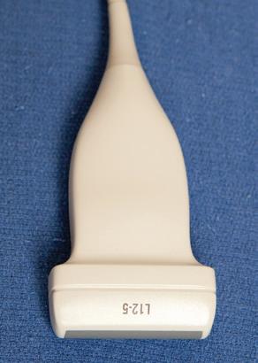
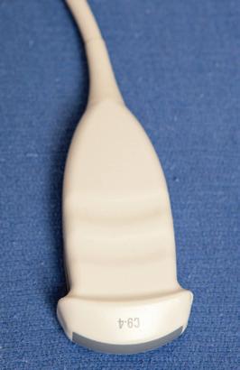
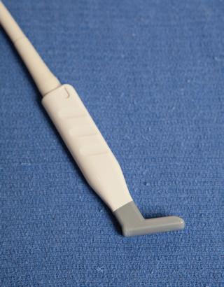
An important consideration in ultrasound imaging is the frequency of the transducer because this determines image quality. A transducer is designated by the range of sound wave frequencies it can produce, described in megahertz (MHz). The higher the frequency, the higher the resolution of the image; however, this is at the expense of sound beam penetration as a result of sound wave absorption.1 In contrast, a low-frequency transducer optimally assesses deeper structures, but it has relatively lower resolution. Transducers may also be designated as linear or curvilinear (Fig. 1.1). With a linear transducer, the sound wave is propagated in a linear fashion parallel to the transducer surface (Video 1.1). This is optimum in evaluation of the musculoskeletal system to assess linear structures, such as tendons, to avoid artifact. A curvilinear transducer may be used in evaluation of deeper structures because this increases the field of view (Video 1.2). A small footprint linear probe is ideal for imaging the hand, ankle, and foot given the contours of these body parts that allow only limited contact with the probe surface (Fig. 1.1C). A small footprint transducer with an offset is helpful when performing procedures on the distal extremities.
The physical size, power, resolution, and cost of ultrasound units vary, and these factors are all related. For example, an ultrasound machine that is approximately 3 × 3 × 4 feet high will likely be very powerful, have many imaging applications, and be able to support multiple transducers, including high-frequency transducers that result in exquisite high-resolution images. Smaller, portable machines are also available, some of which are smaller than a notebook computer. Although these machines cost less than the larger units, there may be tradeoffs related to image resolution and applications. Ultrasound units as small as a handheld electronic device have been introduced, although transducer options may be limited at
this time. As technology advances, these differences have been minimized as the portable ultrasound machines have become more powerful and the larger units have become smaller. It is therefore essential in the selection of a proper ultrasound unit to consider how an ultrasound machine will be used, the size of the structures that need to be imaged, the need for machine portability, and the capabilities of the ultrasound machine.
SCANNING TECHNIQUE
To produce an ultrasound image, the transducer is held on the surface of the skin to image the underlying structures. Ample acoustic transmission gel should be used to enable the sound beam to
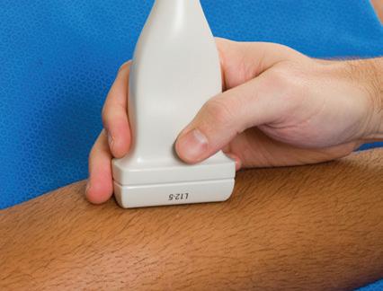
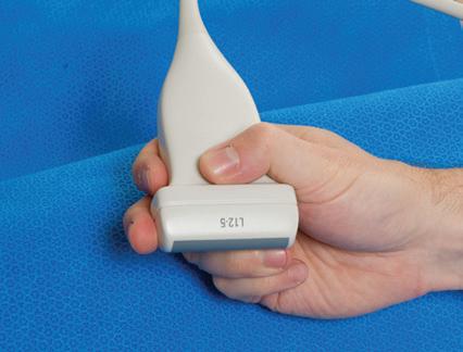
be transmitted from the transducer to the soft tissues and to allow the returning echoes to be converted to the ultrasound image. I prefer a layer of thick transmission gel over a more cumbersome gel standoff pad. Gel that is more like liquid consistency is also less ideal because the gel tends not to stay localized at the imaging site. The transducer should be held between the thumb and fingers of the examiner’s dominant hand, with the end of the transducer near the ulnar aspect of the hand (Fig. 1.2A). The transducer should be stabilized or anchored on the patient with either the small finger or the heel of the imaging hand (Fig. 1.2B). This technique is essential to maintain proper pressure of the transducer on the skin, to avoid involuntary movement of the transducer, and to allow fine adjustments in transducer positioning. Remember that the sound beam
BC
FIGURE 1.1 Transducers. Photographs show linear 12-5 MHz (A), curvilinear 9-4 MHz (B), and compact linear 15-7 MHz (C) transducers.
FIGURE 1.2 Transducer Positioning. A and B, Photographs show that the transducer is stabilized with simultaneous contact of the transducer, the skin surface, and the examiner’s hand.
A B
FIGURE 1.3 Transducer Movements. A, Heel-toe maneuver. B, Toggle maneuver. (Modified from an illustration by Carolyn Nowak, Ann Arbor, Michigan; http://www.carolyncnowak.com/medtech.html.)
emitted from the transducer is focused relative to the short end of the transducer, and side-to-side movement of the transducer should only be a millimeter at a time.
Various terms describe manual movements of the transducer during scanning. The term heel-toe is used when the transducer is rocked or angled along the long axis of the transducer (Fig. 1.3A). The term toggle is used when the transducer is angled from side to side (Fig. 1.3B). With both the heel-toe and toggle maneuvers, the transducer is not moved from its location, but rather the transducer is angled. The term translate is used when the transducer is moved to a new location while maintaining a perpendicular angle with the skin surface. The term sweep is used when the transducer is slid from side to side while maintaining a stable hand position, similar to sweeping a broom.
With regard to ergonomics, proper ultrasound scanning technique can help minimize fatigue and work-related injuries. Anchoring of the transducer to the patient by making contact between the scanning hand and the patient as described earlier decreases muscle fatigue of the examining arm. In addition, making sure that the scanning hand is lower than the ipsilateral shoulder with the elbow close to the body also decreases fatigue of the shoulder. If the examiner uses a chair, one at the appropriate height, preferably with wheels and with some type of back support, will improve
comfort and maneuverability. Last, the ultrasound monitor should be near the patient’s area being scanned so that visualization of both the patient and the monitor can occur while minimizing turning of the head or spine.
There are three basic steps when performing musculoskeletal ultrasound, and these steps are also similar to obtaining an adequate image with magnetic resonance imaging (MRI). The first step is to image the structure of interest in long axis and short axis (if applicable), which depends on knowledge of anatomy. Identification of bone landmarks is helpful for orientation. The second step is to eliminate artifacts, more specifically anisotropy (see later discussion in this chapter) when considering ultrasound. When imaging a structure over bone, the cortex will appear hyperechoic and well defined when the sound beam is perpendicular, which indicates that the tissues over that segment of bone are free of anisotropy. The last step is characterization of pathology. Note the use of bone in two of the previous steps to understand anatomy and the proper imaging plane and to indicate that the sound beam is directed correctly to eliminate anisotropy.
IMAGE APPEARANCE
Once the transducer is placed on the patient’s skin with intervening gel, a rectangular image
(when using a linear transducer) appears on the monitor. The top of the image represents the superficial soft tissues that are in contact with the transducer, and the deeper structures appear toward the lower aspect of the image (Fig. 1.4).
To understand the resulting ultrasound image, consider the sound beam as a plane or slice that extends down from the transducer along its long axis. It is this plane that is portrayed on the image. The left and right sides of the image can represent either end of the transducer, and this can usually be switched by using the left-to-right invert button on the ultrasound machine or by simply rotating the transducer 180 degrees. When imaging a structure in long axis, it is common to have the proximal aspect on the left side of the image and the distal aspect on the right.
Image optimization is essential to maximize resolution and clarity. The first step is to select the proper transducer and frequency. Higherfrequency transducers (10 MHz or greater) optimally evaluate superficial structures, whereas lower-frequency transducers are used for deep structures. Linear transducers are typically used, unless the area of interest is deep, such as the hip region, where a curvilinear transducer may be chosen. After the proper transducer is selected and placed on the patient, the next step is to adjust the depth of the sound beam; this is accomplished by a button or dial on the ultrasound machine. The depth of the sound beam is adjusted until the structure of interest is visible and centered in the image (Fig. 1.5A and B). The next step in optimization is to adjust the focal zones of the ultrasound beam, if present on the ultrasound machine. This feature is typically displayed on the side of the image as a number of cursors or other symbols. It is optimum to reduce the number of focal zones to span the area of interest because increased focal zones will decrease the frame rate that produces a windshield-wiper effect. It is also important to move the depth of the focal zones to the depth where the structure is to be imaged
to optimize resolution (Fig. 1.5C). Some ultrasound machines have a broad focal zone that may not have to be moved. Finally, the overall gain can be adjusted by a knob on the ultrasound machine to increase or decrease the overall brightness of the echoes, which is in part determined by the ambient light in the examination room (Fig. 1.5D). The gain should ideally be set where one can appreciate the ultrasound characteristics of normal soft tissues (as described later in this chapter).
The ultrasound image is produced when the sound beam interacts with the tissues beneath the transducer and this information returns to the transducer. At an interface between tissues where there is a large difference in impedance, the sound beam is strongly reflected, and this produces a very bright echo on the image, which is described as hyperechoic. Examples include interfaces between bone and soft tissues, where the area beneath the interface is completely black from shadowing because no echoes extend beyond the interface. An area on the image that has no echo and is black is termed anechoic, whereas an area with a weak or low echo is termed hypoechoic If a structure is of equal echogenicity to the adjacent soft tissues, it may be described as isoechoic.
SONOGRAPHIC APPEARANCES OF NORMAL STRUCTURES
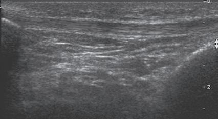
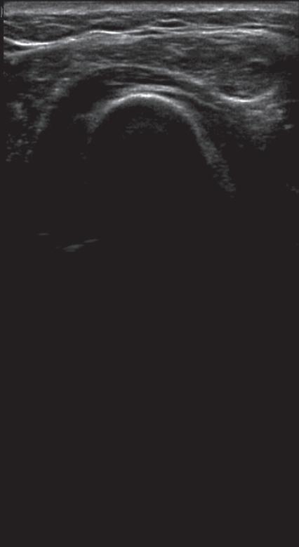
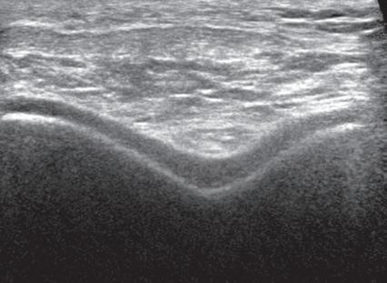
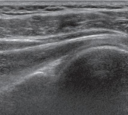
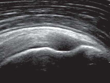
Musculoskeletal structures have characteristic appearances on ultrasound imaging.2 Normal tendons appear hyperechoic with a fiber-like or fibrillar echotexture (see Fig. 1.4).3 At close inspection, the linear fibrillar echoes within a tendon represent the endotendineum septa, which contain connective tissue, elastic fibers, nerve endings, blood, and lymph vessels.3 Continuous tendon fibers are best appreciated when they are imaged long axis to the tendon. On such a long axis image, by convention the proximal aspect is on the left side of the image, with the distal aspect on the right. In short axis, normal hyperechoic tendon fibers appear as bristles of a brush seen on end (see Fig. 1.9A). Normal muscle tissue appears relatively hypoechoic (Fig. 1.6). At closer inspection, the hypoechoic muscle tissue is separated by fine hyperechoic fibroadipose septa or perimysium, which surrounds the hypoechoic muscle bundles. The surface of bone or calcification is typically very hyperechoic, with posterior acoustic shadowing and possibly posterior reverberation if the surface of the bone is smooth and flat (Fig. 1.6). The hyaline cartilage covering the articular surface of bone is hypoechoic and uniform (Fig. 1.7A and B), whereas the fibrocartilage, such as the
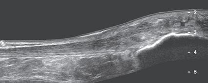
FIGURE 1.4 Normal Patellar Tendon. Ultrasound image of patellar tendon in long axis (arrowheads) shows hyperechoic fibrillar echotexture. P, Patella; T, tibia.
labrum of the hip and shoulder, and the knee menisci are hyperechoic (Fig. 1.7B). Ligaments have a hyperechoic, striated appearance that is more compact compared with tendons (Fig. 1.8). In addition, ligaments are also identified in that they connect two osseous structures. Often normal ligaments may appear relatively hypoechoic when surrounded by hyperechoic subcutaneous fat; however, a compact linear hyperechoic ligament can be appreciated when imaged in long axis perpendicular to the ultrasound beam. Normal peripheral nerves have a fascicular appearance in which the individual nerve fascicles are hypoechoic, surrounded by hyperechoic connective tissue epineurium (Fig. 1.9).4 Hyperechoic fat is typically seen around larger peripheral nerves.
FIGURE 1.5 Optimizing the Ultrasound Image. A, Ultrasound image of forearm musculature shows improper depth, focal zone, and gain. B, Depth is corrected as area of interest is centered in image. C, Focal zone width is decreased and centered at area of interest (arrows). D, Gain is increased.
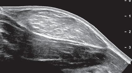
FIGURE 1.6 Muscle. Ultrasound image of brachialis and biceps brachii muscles in long axis shows hypoechoic muscle and hyperechoic fibroadipose septa (arrows). H, Humerus.
FIGURE 1.7 Cartilage. A, Ultrasound image transverse over the distal anterior femur shows hypoechoic hyaline cartilage (arrowheads) F, Femur. B, Ultrasound image of infraspinatus in long axis (I) shows a hyperechoic fibrocartilage glenoid labrum (arrowheads) and hypoechoic hyaline cartilage (curved arrow). Note hyperechoic epidermis and dermis (E/D), and adjacent deeper hypoechoic hypodermis with hyperechoic septa. G, Glenoid; H, humerus.
FIGURE 1.8 Tibial Collateral Ligament. Ultrasound image of tibial collateral ligament of the knee in long axis shows compact fibrillar echotexture (arrowheads). F, Femur; m, meniscus; T, tibia.
In short axis, peripheral nerves display a honeycomb or speckled appearance, which assists in their identification. Because peripheral nerves have a relatively mixed hyperechoic and hypoechoic echotexture, their appearance changes relative to the adjacent tissues. For example, the median nerve in the forearm, when surrounded by hypoechoic muscle, appears relatively hyperechoic; in contrast, more distally in the carpal tunnel, when it is surrounded by hyperechoic tendon, the median nerve appears relatively hypoechoic (see Fig. 5.4D). The epidermis and dermis collectively appear hyperechoic, whereas the hypodermis shows hypoechoic fat and hyperechoic fibrous septa (see Fig. 1.7).
SONOGRAPHIC ARTIFACTS
One should be familiar with several artifacts common to musculoskeletal ultrasound.5 One
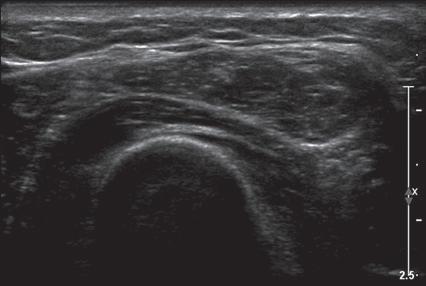
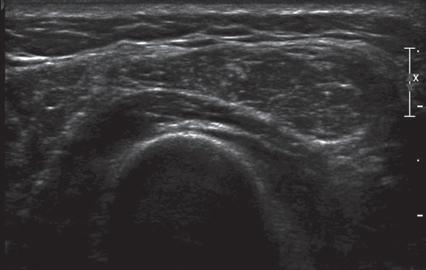
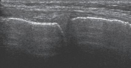
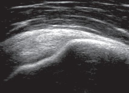
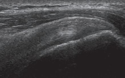
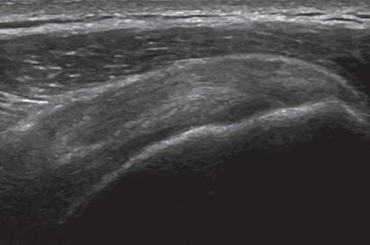
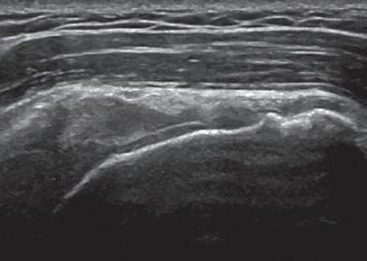
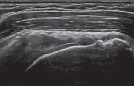
such artifact is anisotropy 6 When a tendon is imaged perpendicular to the ultrasound beam, the characteristic hyperechoic fibrillar appearance is displayed. However, when the ultrasound beam is angled as little as 2 to 3 degrees relative to the long axis of such a structure, the normal hyperechoic appearance is lost; the tendon becomes more hypoechoic with increased insonation angle (Figs. 1.10 to 1.13). A tissue is anisotropic if its properties change when measured from different directions. This variation of ultrasound interaction with fibrillar tissues involves tendons and ligaments and, to a lesser extent, muscle. Because abnormal tendons and ligaments may also appear hypoechoic, it is important to focus on that segment of tendon or ligament that is perpendicular to the ultrasound beam, to exclude anisotropy. With a curved structure, such as the distal aspect of the supraspinatus tendon, the transducer is continually repositioned or angled to exclude anisotropy as the cause of a hypoechoic tendon segment (Fig. 1.11 and Video 1.3). Anisotropy is noted both in long axis and short axis of ligaments and tendons (Video 1.4), but it occurs when the sound beam is angled relative to the long axis of a structure (Fig. 1.12). Therefore, to correct for anisotropy, the transducer is angled along the long axis of the imaged tendon or ligament; when imaging a tendon in long axis, the transducer is angled as a heel-toe maneuver (see Fig. 1.3A and Video 1.5), whereas in short axis, the transducer is toggled (see Fig. 1.3B and Video 1.6). Anisotropy can be used to one’s advantage in identification of a hyperechoic tendon or ligament in close proximity to hyperechoic soft tissues, such as
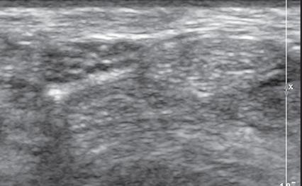
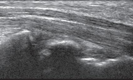
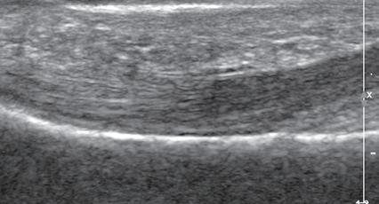
FIGURE 1.10 Anisotropy. Ultrasound image of flexor tendons of the finger in long axis shows normal tendon hyperechogenicity (arrowheads) becoming more hypoechoic as the tendon becomes oblique relative to the sound beam (open arrows). P, Proximal phalanx.
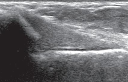
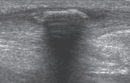
involved interface. Examples of structures that produce shadowing include interfaces with bone or calcification (Fig. 1.14), some foreign bodies (see Chapter 2), and gas. An object with a small radius of curvature or a rough surface will display a clean shadow, whereas an object with a large radius of curvature and a smooth surface will display a dirty shadow (resulting from superimposed reverberation echoes).8 Refractile shadowing may also occur at the edge of some structures, such as a foreign body or the end of a torn Achilles or patellar tendon (Fig. 1.15).9
in the ankle and wrist. When imaging a tendon in short axis, toggling the transducer will cause the tendon to become hypoechoic, thus allowing its distinction from the adjacent hyperechoic fat that does not demonstrate anisotropy (Fig. 1.12). Once the tendon is identified, anisotropy must be corrected to exclude pathology. Anisotropy is also helpful in identification of some ligaments, such as in the ankle, because they are often adjacent to hyperechoic fat (Fig. 1.13). In addition, hyperechoic tendon calcifications can be made more conspicuous when they are surrounded by hypoechoic tendon from anisotropy with angulation of the transducer (see Fig. 3.63). When performing an interventional procedure, it is anisotropy that causes the needle to become less conspicuous when the needle is not perpendicular to the sound beam (see Fig. 9.8).
Another important artifact is shadowing. This occurs when the ultrasound beam is reflected, absorbed, or refracted.7 The resulting image shows an anechoic area that extends deep from the
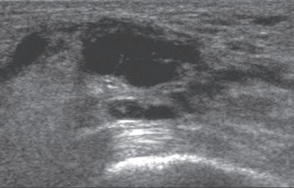
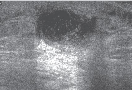
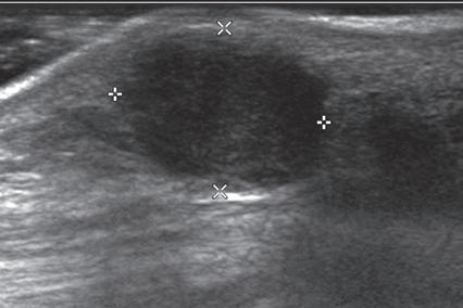
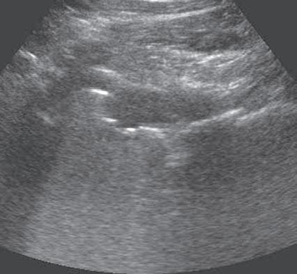
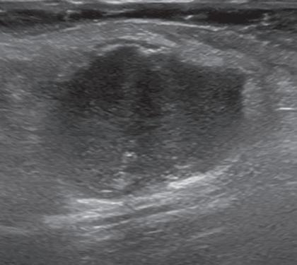
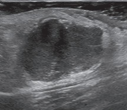
Another type of artifact is posterior acoustic enhancement or increased through-transmission. This occurs during imaging of fluid (Figs. 1.16 and 1.17) and some solid soft tissue tumors, such as peripheral nerve sheath tumors (see Fig. 2.59) and pigmented villonodular tenosynovitis (giant cell tumors of tendon sheath) (Fig. 1.18).10 In these situations, the sound beam is relatively less attenuated compared with the adjacent tissues; therefore, the deeper soft tissues will appear relatively hyperechoic compared with the adjacent soft tissues.7
Another artifact with musculoskeletal implications is posterior reverberation. This occurs when the surface of an object is smooth and flat, such as a metal object or the surface of bone. In this situation, the sound beam reflects back and forth between the smooth surface and the transducer and produces a series of linear reflective echoes that extend deep to the structure.7 If the series of reflective echoes is more continuous deep to the structure, the term ring-down artifact is used, as may be seen with metal surfaces (Fig. 1.19). Ultrasound is ideal in evaluation of structures immediately overlying metal hardware because this reverberation artifact occurs deep to the hardware without obscuring the superficial soft tissues. Related to posterior reverberation is the
FIGURE 1.9 Median Nerve. A, Ultrasound image of median nerve in short axis (arrowheads) shows individual hypoechoic nerve fascicles (arrow) and the adjacent hyperechoic flexor carpi radialis tendon (open arrows). B, Ultrasound image of median nerve in long axis (arrowheads) shows hypoechoic nerve fascicles (arrow). Note the adjacent fibrillar flexor digitorum (F) and palmaris longus (P) tendons. C, Capitate; L, lunate; R, radius.
FIGURE 1.11 Anisotropy. Ultrasound images of distal supraspinatus tendon in long axis (S) shows an area of hypoechoic anisotropy (curved arrow) (A), where the tendon fibers become oblique to the sound beam, which is eliminated (B) when the transducer is repositioned so that the tendon fibers are perpendicular to the sound beam. H, Humerus.
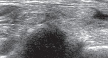
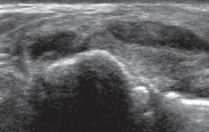
FIGURE 1.12 Anisotropy. Ultrasound images of tibialis posterior (P) and flexor digitorum longus (F) tendons in short axis at the ankle show normal tendon hyperechogenicity (A) and hypoechoic anisotropy (open arrows) (B), when angling or toggling the transducer along the long axis of the tendons, thus aiding in identification of tendons relative to surrounding hyperechoic fat.
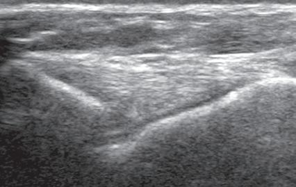
FIGURE 1.13 Anisotropy. Ultrasound images of anterior talofibular ligament in long axis (arrowheads) in the ankle show normal ligament hyperechogenicity (A) and hypoechoic anisotropy (open arrows) (B), when angling the transducer along the long axis of the ligament, thus aiding in identification of ligament relative to surrounding hyperechoic fat. F, Fibula; T, talus.
FIGURE 1.14 Shadowing. Ultrasound image of Achilles tendon in long axis (arrowheads) shows hyperechoic ossification (arrows) with posterior acoustic shadowing (open arrows).
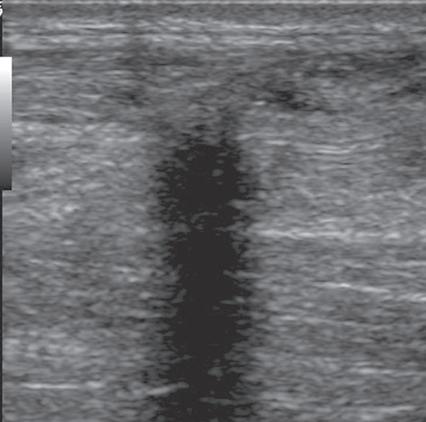
FIGURE 1.15 Refractile Shadowing. Ultrasound image of Achilles tendon in long axis (arrowheads) shows shadowing (open arrows) at the site of a full-thickness tear (curved arrow).
FIGURE 1.16 Increased Through-Transmission. Ultrasound image of a ganglion cyst (arrows) in the ankle shows increased through-transmission (open arrows). t, Flexor hallucis longus tendon.
FIGURE 1.17 Increased Through-Transmission. Ultrasound image of a soft tissue abscess (arrows) in the shoulder shows increased through-transmission (open arrows).
FIGURE 1.18 Increased Through-Transmission. Ultrasound image of a pigmented villonodular tenosynovitis (giant cell tumor of the tendon sheath) (between × and + cursors) shows increased through-transmission (open arrows).
FIGURE 1.19 Ring-Down Artifact. Ultrasound image in long axis to the femoral component of a total hip arthroplasty shows the hyperechoic metal surface of the arthroplasty (arrows) and posterior ring-down artifact (open arrows). Note the overlying joint fluid (f) and adjacent native femur (F).
comet-tail artifact, such as that seen with soft tissue gas (Fig. 1.20), which appears as a short segment of posterior bright echoes that narrows further from the source of the artifact.
One additional artifact to consider is beam-width artifact. This is essentially analogous to volume averaging and occurs if the ultrasound beam is too wide relative to the object being imaged. An example is imaging of a small calcification in which the relatively large beam width may eliminate shadowing. This effect can be reduced by adjusting the focal zone to the level of the object of interest.7
MISCELLANEOUS ULTRASOUND TECHNIQUES
Several ultrasound techniques or applications available with some ultrasound machines can
FIGURE 1.20 Comet-Tail Artifact. Ultrasound over an infected subacromial-subdeltoid bursa (arrows) shows hyperechoic foci of gas with comet-tail artifact (arrowheads). H, Greater tuberosity of the humerus.
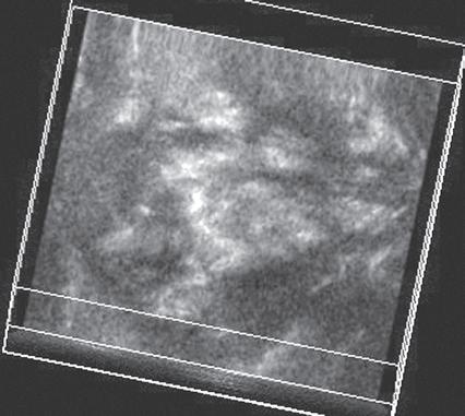
enhance scanning and diagnostic capabilities. One such method is spatial compound sonography 11 Unlike conventional ultrasound, sound beams with spatial compound sonography are produced at several different angles, with information combined to form a single ultrasound image. This improves tissue plane definition, but it has a smoothing effect, and motion blur is more likely because frames are compounded (Fig. 1.21). The use of spatial compounding may alter the artifact produced by a foreign body, which may change its conspicuity (see Fig. 2.47).
Another ultrasound technique is tissue harmonic imaging. Unlike conventional ultrasound, which receives only the fundamental or transmitted frequency to produce the image, with tissue harmonic imaging, harmonic frequencies produced during ultrasound beam propagation through tissues are used to produce the image. This technique assists in evaluation of deep structures and also improves joint and tendon surface visibility.12,13 The technique may more clearly delineate the edge of a soft tissue mass (Fig. 1.22) or a fluid-filled tendon tear (Fig. 1.23). One pitfall is that hypoechoic tendinosis may appear more anechoic with tissue harmonic imaging and simulate a tendon tear.
One helpful technique available on some ultrasound machines is extended field of view. With this technique, an ultrasound image is produced by combining image information obtained during real-time scanning. This allows imaging of an entire muscle from origin to insertion; it is helpful in measuring large abnormalities (e.g., tumor or tendon tear) and in displaying and communicating ultrasound findings (Figs. 1.24 and 1.25).14 An alternative to extended field of view imaging that is available on some ultrasound equipment is the split-screen function, which essentially joins two images on the display screen that doubles the field of view.
A B
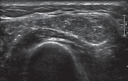
FIGURE 1.21 Spatial Compounding. Ultrasound images of the supraspinatus tendon without (A) and with (B) spatial compounding show softening of the image in B.
AB
1.22 Tissue Harmonic Imaging. Ultrasound images of a recurrent giant cell tumor (arrowheads) without (A) and with (B) tissue harmonic imaging show increased definition of the mass borders in B. Note posterior increased through-transmission.
A B
FIGURE 1.23 Tissue Harmonic Imaging. Ultrasound images of full-thickness supraspinatus tendon tear in long axis (arrows) without (A) and with (B) tissue harmonic imaging show clearer distinction of retracted tendon stump (left arrow) because intervening fluid is more hypoechoic.
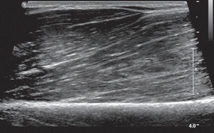
FIGURE 1.24 Extended Field of View. Ultrasound image of the Achilles tendon in long axis shows hypoechoic and enlarged tendinosis (open arrows) and retro-Achilles bursitis (curved arrow). Note the normal Achilles thickness proximally (arrowheads). C, Calcaneus.
A number of ultrasound techniques are relatively new, and their practical musculoskeletal applications are still being defined. One such technique is three-dimensional ultrasound, which acquires data as a volume (either mechanically or
1.25 Extended Field of View. Ultrasound image shows full extent of a lipoma (between arrows).
freehand) and thus enables reconstruction at any imaging plane (Fig. 1.26). This technique has been used to characterize rotator cuff tears and to quantify a volume of tissue such as tumor or synovial hypertrophy.15,16 An additional technique
FIGURE
FIGURE
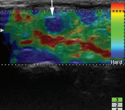
area below white arrow). Note that hard tissues are displayed in blue and soft tissues in red. (Courtesy
Michigan.)
is fusion imaging, in which real-time ultrasound imaging can be superimposed on computed tomography (CT) or MRI; this has been used to assist with needle guidance for sacroiliac joint injections.17 One last technique is sonoelastography, which is used to assess the elastic properties of tissue. The three types of sonoelastography include compression elastography (using manual compression), shear wave elastography (using a directional shear wave), and transient elastography (using a short pulse).18 With compression elastography, manual compression of tissue produces strain or displacement within the tissue. Displacement is less when tissue is hard; it is displayed as blue on the ultrasound image, whereas soft tissue is displayed as red (Fig. 1.27). With regard to musculoskeletal applications, normal tendons appear as blue, whereas areas of tendinopathy, such as of the Achilles tendon or common extensor tendon of the elbow, appear as red.16,19-22 With shear wave and transient elastography, the velocity of the shear wave is measured to determine elasticity and has the advantage of less operator dependence and ability to produce qualitative and quantitative information.18,23
COLOR AND POWER DOPPLER
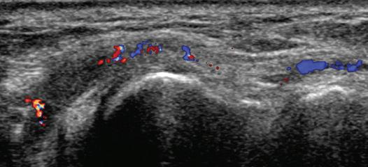
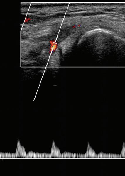
Most ultrasound machines include color and power Doppler imaging capabilities, with possible spectral waveform analysis. Ultrasound uses the Doppler effect, in which the sound frequency of an object changes as the object travels toward or away from a point of reference, to obtain information about blood flow. Color flow imaging shows
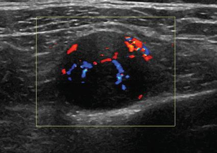
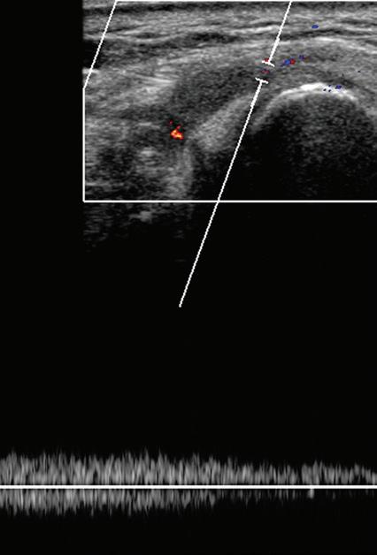
colored blood flow superimposed on a gray-scale image, in which two colors such as red and blue represent flow toward and away from the transducer, respectively (Fig. 1.28).24 Pulsed-wave or duplex Doppler ultrasound displays an ultrasound image and waveform (Fig. 1.29). There are important considerations to optimize the Doppler ultrasound. Reducing the width of the field of view and increasing the frame rate are helpful. To correct for aliasing (when the Doppler shift frequency of blood is greater than the detected frequency, which causes an error in frequency measurement), one can increase the pulse repetition frequency, lower the ultrasound frequency, or increase the angle between the sound beam
FIGURE 1.26 Three-Dimensional Imaging. Ultrasound image reconstructed in the coronal plane shows a heterogeneous thigh sarcoma (arrowheads).
FIGURE 1.27 Ultrasound Elastography: Foreign Body Granuloma. Ultrasound image of common extensor tendon elbow shows suture granuloma (blue mass-like
Y. Morag, Ann Arbor,
FIGURE 1.28 Color Doppler: Schwannoma. Color Doppler ultrasound image shows increased blood flow in hypoechoic peripheral nerve sheath tumor.
1.29 Color Doppler: Radial Artery Thrombosis. A, Color Doppler ultrasound image in long axis to the radial artery (arrowheads) at the wrist shows hypoechoic thrombus and diminished blood flow. B, Pulsed-wave Doppler shows the loss of normal arterial flow at the site of thrombus (B) and distal reconstitution from the deep palmar arch (C).
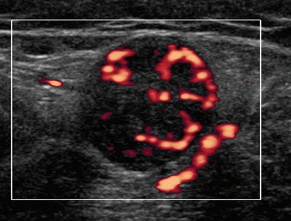
and the flow direction toward perpendicular. Power Doppler is another method of color Doppler ultrasound that is generally considered more sensitive to blood flow (it shows small vessels and slow flow rates) compared with conventional color Doppler, although significant variability exists depending on the ultrasound machine.25 Unlike conventional color Doppler, power Doppler assigns a color to blood flow regardless of direction (Fig. 1.30) and is extremely sensitive to movement of the transducer, which produces a flash artifact. The color gain should be optimally adjusted for Doppler imaging to avoid artifact if the setting
is too sensitive and for false-negative flow if sensitivity is too low. To optimize power Doppler imaging, set the color background (without the gray-scale displayed) so that the lowest level of color nearly uniformly is present, with only minimal presence of the next highest color level.26
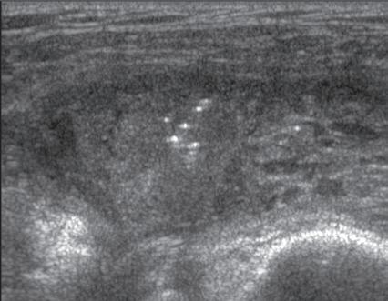
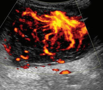
Increased blood flow on color or power Doppler imaging may occur with increased perfusion, inflammation, and neovascularity. In imaging soft tissues, color and power Doppler imaging are used to confirm that an anechoic tubular structure is a blood vessel and to confirm blood flow. When a mass is identified, increased blood
FIGURE
flow may suggest neovascularity, possibly from malignancy (Fig. 1.31).27 Although the finding is nonspecific, a tumor without flow is more likely to be benign, and malignant tumors usually demonstrate increased flow and irregular vessels.28 With regard to superficial lymph nodes, either no flow or hilar flow is more common with benign lymph node enlargement, and spotted, peripheral, or mixed patterns of flow are more common with malignant lymph node enlargement (see Chapter 2).29 Color or power Doppler imaging is also helpful in the differentiation between complex fluid and a mass or synovitis; the former typically has no internal flow, and the latter may show increased flow.30 After treatment for inflammatory
arthritis, color and power Doppler imaging can show interval decrease in flow, which would indicate a positive response.31 It is also important to use color Doppler imaging during a biopsy to ensure that major vessels are avoided.
DYNAMIC IMAGING
One significant advantage of ultrasound over other static imaging methods, such as radiography, CT, and conventional MRI, is the dynamic capability On a basic level, ultrasound evaluation can be directly guided by a patient’s history, symptoms, and findings at physical examination. In fact, regardless of the protocol followed for imaging a joint, it is essential that ultrasound is focused during one aspect of the examination over any area of point tenderness or focal symptoms.32 Once ultrasound examination is begun, the patient can directly provide feedback with regard to pain or other symptoms with transducer pressure over an ultrasound abnormality. When a patient has a palpable abnormality, direct palpation under ultrasound visualization will ensure that the imaged abnormality corresponds to the abnormality. Graded compression also provides additional information about soft tissue masses; lipomas are often soft and pliable (see Video 2.7).
In the setting of a rotator cuff tear, compression can help demonstrate the volume loss associated with a full-thickness tear (see Video 3.23). With regard to peripheral nerves, transducer pressure over a nerve at the site of entrapment can reproduce symptoms and help to guide the examination. Transducer pressure over a stump neuroma is also used to determine if a neuroma is causing symptoms. If during examination there is question of a complex fluid collection, variable transducer pressure can demonstrate swirling of internal debris and displacement, which indicates a fluid component (see Videos 6.14 to 6.16). In contrast, synovial hypertrophy would show only minimal compression without internal movement of echoes, with possible additional findings of flow on color and power Doppler imaging (see Video 8.5).
Dynamic imaging is also important in evaluation of complete full-thickness muscle, tendon, or ligament tear. When a full-thickness muscle or tendon tear is suspected, the muscle-tendon unit may be actively contracted or passively moved during imaging in long axis (see Videos 7.15 and 8.46). Demonstration of muscle or tendon stumps that move away from each other during this dynamic maneuver at the site of the tear indicates full-thickness extent. With regard to ligament tear, a joint can be stressed while imaging in long axis to the ligament to evaluate for ligament
FIGURE 1.30 Power Doppler: Schwannoma. Power Doppler ultrasound image shows increased blood flow in hypoechoic peripheral nerve sheath tumor.
FIGURE 1.31 Power Doppler: B-Cell Lymphoma. Power
Doppler ultrasound image shows increased blood flow in hypoechoic lymphoma (arrowheads). Note posterior increased through-transmission.
disruption and abnormal joint space widening. One example of this is applying valgus stress to the elbow when evaluating for ulnar collateral ligament tear (see Videos 4.15 to 4.17).
One last application of dynamic imaging is in evaluation of an abnormality that is present only when an extremity is moved or positioned in a particular manner. Examples of this include evaluation of the long head of biceps brachii tendon for subluxation or dislocation with shoulder external rotation (see Video 3.43), the ulnar nerve (see Video 4.21) and snapping triceps syndrome with elbow flexion (see Video 4.22), the peroneal tendon with dorsiflexion and eversion of the ankle (see Videos 8.30 to 8.33), and snapping hip syndrome (see Videos 6.18 to 6.21). Muscle contraction is often required for the diagnosis of muscle hernia (see Videos 8.40 to 8.42). Dynamic imaging of a patient during Valsalva maneuver is an essential component in evaluation for inguinal region hernia (see Videos 6.26 to 6.31). In addition to the foregoing examples, if the patient has any complaints that occur with a specific movement or position, the ultrasound transducer can be
placed over the abnormal area, and the patient can be asked to re-create the symptom.
SELECT REFERENCES
5. Gimber LH, Melville DM, Klauser AS, et al: Artifacts at musculoskeletal US: resident and fellow education feature. Radiographics 36(2):479–480, 2016.
12. Anvari A, Forsberg F, Samir AE: A primer on the physical principles of tissue harmonic imaging. Radiographics 35(7):1955–1964, 2015.
16. Klauser AS, Peetrons P: Developments in musculoskeletal ultrasound and clinical applications. Skeletal Radiol (Sep 3), 2009.
18. Klauser AS, Miyamoto H, Bellmann-Weiler R, et al: Sonoelastography: musculoskeletal applications. Radiology 272(3):622–633, 2014.
24. Boote EJ: AAPM/RSNA physics tutorial for residents: topics in US: Doppler US techniques: concepts of blood flow detection and flow dynamics. Radiographics 23(5):1315–1327, 2003.
The complete references for this chapter can be found on www.expertconsult.com
REFERENCES
1. Curry TS, Dowdey JE, Murry RC: Christensen’s physics of diagnostic radiology, ed 4, Philadelphia, 1990, Lea and Febiger.
2. Erickson SJ: High-resolution imaging of the musculoskeletal system. Radiology 205(3):593–618, 1997.
3. Martinoli C, Derchi LE, Pastorino C, et al: Analysis of echotexture of tendons with US. Radiology 186(3): 839–843, 1993.
4. Silvestri E, Martinoli C, Derchi LE, et al: Echotexture of peripheral nerves: correlation between US and histologic findings and criteria to differentiate tendons. Radiology 197(1):291–296, 1995.
5. Gimber LH, Melville DM, Klauser AS, et al: Artifacts at musculoskeletal US: resident and fellow education feature. Radiographics 36(2):479–480, 2016.
6. Crass JR, van de Vegte GL, Harkavy LA: Tendon echogenicity: ex vivo study. Radiology 167(2):499–501, 1988.
7. Scanlan KA: Sonographic artifacts and their origins. AJR Am J Roentgenol 156(6):1267–1272, 1991.
8. Rubin JM, Adler RS, Bude RO, et al: Clean and dirty shadowing at US: a reappraisal. Radiology 181(1):231–236, 1991.
9. Hartgerink P, Fessell DP, Jacobson JA, et al: Fullversus partial-thickness Achilles tendon tears: sonographic accuracy and characterization in 26 cases with surgical correlation. Radiology 220(2): 406–412, 2001.
10. Reynolds DL, Jr, Jacobson JA, Inampudi P, et al: Sonographic characteristics of peripheral nerve sheath tumors. AJR Am J Roentgenol 182(3):741–744, 2004.
11. Lin DC, Nazarian LN, O’Kane PL, et al: Advantages of real-time spatial compound sonography of the musculoskeletal system versus conventional sonography. AJR Am J Roentgenol 179(6):1629–1631, 2002.
12. Anvari A, Forsberg F, Samir AE: A primer on the physical principles of tissue harmonic imaging. Radiographics 35(7):1955–1964, 2015.
13. Strobel K, Zanetti M, Nagy L, et al: Suspected rotator cuff lesions: tissue harmonic imaging versus conventional US of the shoulder. Radiology 230(1): 243–249, 2004.
14. Lin EC, Middleton WD, Teefey SA: Extended field of view sonography in musculoskeletal imaging. J Ultrasound Med 18(2):147–152, 1999.
15. Kang CH, Kim SS, Kim JH, et al: Supraspinatus tendon tears: comparison of 3D US and MR arthrography with surgical correlation. Skeletal Radiol 38(11):1063–1069, 2009.
16. Klauser AS, Peetrons P: Developments in musculoskeletal ultrasound and clinical applications. Skeletal Radiol (Sep 3), 2009.
17. Klauser AS, De Zordo T, Feuchtner GM, et al: Fusion of real-time US with CT images to guide sacroiliac joint injection in vitro and in vivo. Radiology 256(2):547–553, 2010.
18. Klauser AS, Miyamoto H, Bellmann-Weiler R, et al: Sonoelastography: musculoskeletal applications. Radiology 272(3):622–633, 2014.
19. De Zordo T, Chhem R, Smekal V, et al: Real-time sonoelastography: findings in patients with symptomatic Achilles tendons and comparison to healthy volunteers. Ultraschall Med 31(4):394–400, 2010.
20. De Zordo T, Fink C, Feuchtner GM, et al: Realtime sonoelastography findings in healthy Achilles tendons. AJR Am J Roentgenol 193(2):W134–W138, 2009.
21. De Zordo T, Lill SR, Fink C, et al: Real-time sonoelastography of lateral epicondylitis: comparison of findings between patients and healthy volunteers. AJR Am J Roentgenol 193(1):180–185, 2009.
22. Klauser AS, Faschingbauer R, Jaschke WR: Is sonoelastography of value in assessing tendons? Semin Musculoskelet Radiol 14(3):323–333, 2010.
23. Arda K, Ciledag N, Aktas E, et al: Quantitative assessment of normal soft-tissue elasticity using shear-wave ultrasound elastography. AJR Am J Roentgenol 197(3):532–536, 2011.
24. Boote EJ: AAPM/RSNA physics tutorial for residents: topics in US: Doppler US techniques: concepts of blood flow detection and flow dynamics. Radiographics 23(5):1315–1327, 2003.
25. Torp-Pedersen S, Christensen R, Szkudlarek M, et al: Power and color Doppler ultrasound settings for inflammatory flow: impact on scoring of disease activity in patients with rheumatoid arthritis. Arthritis Rheumatol 67(2):386–395, 2015.
26. Bude RO, Rubin JM: Power Doppler sonography Radiology 200(1):21–23, 1996.
27. Bodner G, Schocke MF, Rachbauer F, et al: Differentiation of malignant and benign musculoskeletal tumors: combined color and power Doppler US and spectral wave analysis. Radiology 223(2): 410–416, 2002.
28. Belli P, Costantini M, Mirk P, et al: Role of color Doppler sonography in the assessment of musculoskeletal soft tissue masses. J Ultrasound Med 19(12):823–830, 2000.
29. Wu CH, Shih JC, Chang YL, et al: Two-dimensional and three-dimensional power Doppler sonographic classification of vascular patterns in cervical lymphadenopathies. J Ultrasound Med 17(7):459–464, 1998.
30. Breidahl WH, Stafford Johnson DB, Newman JS, et al: Power Doppler sonography in tenosynovitis: significance of the peritendinous hypoechoic rim. J Ultrasound Med 17(2):103–107, 1998.
31. Ribbens C, Andre B, Marcelis S, et al: Rheumatoid hand joint synovitis: gray-scale and power Doppler US quantifications following anti-tumor necrosis factor-alpha treatment: pilot study. Radiology 229(2): 562–569, 2003.
32. Jamadar DA, Jacobson JA, Caoili EM, et al: Musculoskeletal sonography technique: focused versus comprehensive evaluation. AJR Am J Roentgenol 190(1):5–9, 2008.