A cknowledgments
Without the guidance and support of my mentors, this work would not have been possible. I credit the visionary leadership of our chair, Vijay Rao, for the fertile clinical and academic environment of our department in which I was able to compose this work.
I largely owe my interest, aptitude, and understanding of MRI to Don Mitchell. His book, MRI Principles, attracted me to MRI and TJU for fellowship training and provided the foundation of my understanding of MRI physics. With his own unique brand of mentorship, George Holland also endowed me with a deeper appreciation and understanding of body MRI.
The excellent Jefferson technologists at our Center City and Methodist campuses and outlying outpatient imaging centers deserve recognition for optimizing and acquiring the clinical images, which are the backbone of this text. We’re indebted to you for providing a veritable cornucopia of technically superior images with which to adorn the book and animate the text.
We’d be remiss if we didn’t credit our stellar residents and fellows with challenging us on a daily basis with their intellectual curiosity and helping us to better understand the needs of the readership.
-Christopher G. Roth
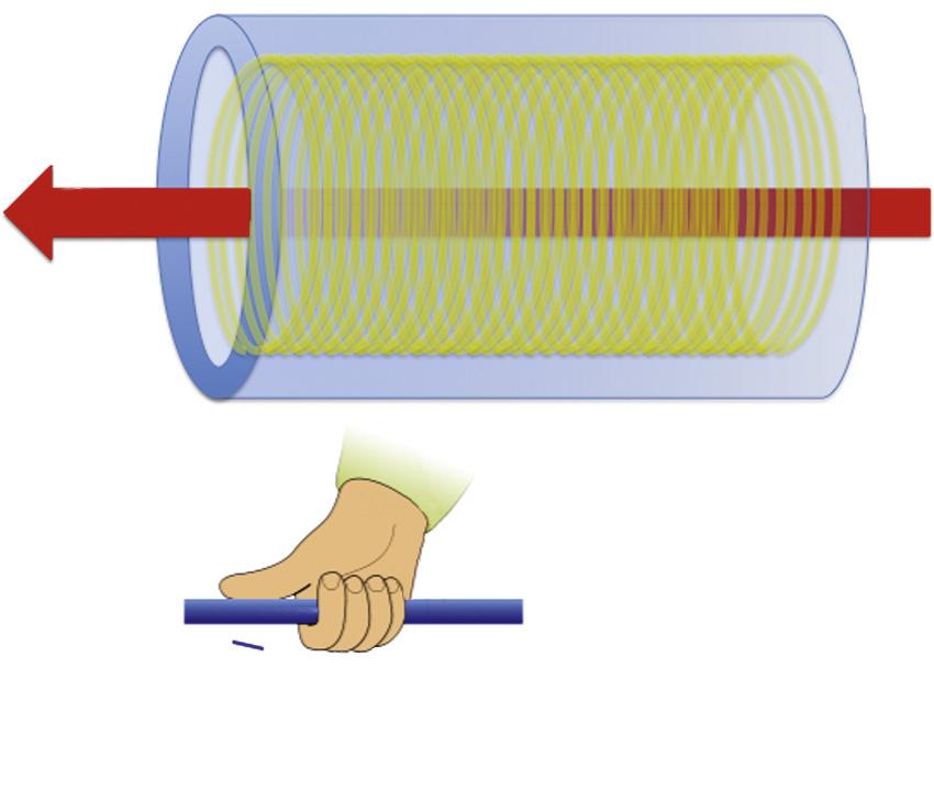
wire (ie, niobium-titanium or niobium-tin), which is supercooled (with liquid helium or nitrogen) ( Fig. 1.4 ). 2 Superconducting wire that is cooled appropriately permits the flow of electric current with virtually no resistance. By virtue of the thumb rule (officially Ampere’s Law), the result is a magnetic field oriented along the axis of the solenoid (B 0).
Rf System
Another key component of the MRI apparatus is the Rf transmitter system that generates the Rf pulse exciting the magnetized protons. Four components constitute the Rf transmitter system: the frequency synthesizer, the digital envelope of Rfs, a high-power amplifier, and an antenna in the form of a “coil.” The net effect is
generation of an Rf pulse to excite the magnetized protons by exploiting MR.
In order to explain this process and the concept of MR, a basic understanding of nuclear physics and magnetism is necessary. As mentioned earlier, protons in a magnetic field become aligned, and the body becomes magnetized. In addition to aligning parallel or anti-parallel to B0, the protons rotate—or precess—around their magnetic axis, referred to as magnetic spin (see Fig. 1.2). The angular momentum (ω0) and, accordingly, the frequency of precession (f0) vary according to the strength of the magnetic field (B0) and the gyromagnetic ratio (γ), which is a function of the specific properties of the nucleus—expressed by the Larmor equation:
ω0 =γB0 /2π which simplifies to f0 =γB0
Magnetic spin precessing at the frequency of the Rf pulse will absorb energy and move to the higher energy state. Thereafter, excited protons “relax,” emitting the absorbed energy and returning to their original low-energy state. The emitted Rf energy constitutes the signal that ultimately generates an MR image. Conceptually, the NMV is aligned parallel to B0 preceding the Rf excitation pulse. The Rf excitation pulse shifts spins into the higher energy state and the NMV away from the longitudinal axis of B0 into the transverse plane. So, initially, the NMV is longitudinal—parallel to B0—and tilted by the Rf excitation pulse away from B0 into the transverse plane (Fig. 1.5). The transverse component of the spin vector ultimately constitutes the MR signal.3
B0
magnetic vector
FIG. 1.3 The net magnetic vector (NMV) concept.
Current
The hand grip or thumb rule
B
B0
FIG. 1.4 Schematic of a superconducting magnet.
Spins moving to higher energy state More spins in higher energy state
The Gradient System
A gradient system (a spatially varying magnetic field superimposed on spatially uniform B0) distorts the magnetic environment in order to selectively excite a region—or slice—of tissue at a time to facilitate image generation and to send spatial information into the excited volume of protons. The gradient system includes three separate gradients each designed for its designated orthogonal plane: x, y, and z (Fig. 1.6). Each gradient is a coil through which current passes to induce changes in B0 and a linear variation in the main magnetic field (B0) along its respective axis. In other words, a gradient alters the B0 along a scale such that the magnetic field strength at one end of the gradient is stronger than the other (see Fig. 1.6).
The z—or slice-select—gradient (G z or G s) establishes the environment in which a specific slice of protons is excited. By varying the magnetic field strength along the axis of B 0, the slice-select gradient concordantly varies the precessional frequency of the protons along the B 0 axis. Consequently, an Rf pulse emitted with a narrow range of frequencies excites only a thin slice of protons ( Fig. 1.7 ). The narrow range of frequencies included in the Rf pulse— the transmit bandwidth—thereby determines the thickness of the excited slice of protons. This slice of excited protons ultimately constitutes the MR image.
X- and y-gradients incorporate additional spatial information into the excited slice of protons, allowing the emitted MR energy to be converted into an MR image. The gradients are applied in axes orthogonal to the slice-select gradient. The x-gradient—or frequency-encoding gradient or readout gradient (Gx or Gf)—applied perpendicular to B0—functions analogously to the slice-select gradient. By orchestrating a gradient magnetic field, spins vary in precessional frequency along a spectrum from one end of the excited slice of protons to the other (Fig. 1.8). Because spins precessing at different frequencies result in destructive interference, which reduces the emitted signal, the frequencyencoding gradient is applied in two separate phases, or lobes—the dephasing and rephasing lobes (Fig. 1.9).
The y-gradient—or phase-encoding gradient (Gy or Gp)—encodes spatial information into the excited slice of protons along the final orthogonal axis. Applied briefly, the phase-encoding gradient induces a magnetic field gradient along the final orthogonal axis such that spins at one end transiently spin faster than spins at the opposite end (Fig. 1.10). Thereafter, when turned off, the spins retain their differential phase varying across the phase-encoding direction. This phase variation constitutes the spatial information along the phase-encoding axis, which is incorporated into the emitted resonance signal.
NMV
NMV
Rf excitation pulse
B0
FIG. 1.5 Net magnetic vector (NMV) tilted by the radiofrequency (Rf) excitation pulse.
free precession (SSFP), and echo planar imaging (EPI).4 For a brief discussion of different pulse sequences, refer to the upcoming section in this chapter; for more detail on this subject, refer to texts dedicated to MRI physics—MRI Principles, D. G. Mitchell; MRI Basic Principles and Applications, M. A. Brown and R. C. Semelka; The MRI Manual, R. B. Lufkin; MRI: The Basics, R. H. Hashemi, W. G. Bradley Jr., and C. J. Lisanti; and MRI in Practice, C. Westbrook and C. Kaut.5,6,7,8,9
The Receiver System
The next pertinent hardware component is the system designed to receive or capture the emitted resonance energy. In review, the components discussed to this point include the main magnetic field (B0), the Rf transmitter system, and the gradient magnetic field system. The receiver system includes a receiver coil, a receiver amplifier, and an analog-to-digital converter (ADC). A component of the Rf system previously mentioned—the transmit coil—often doubles as the receiver coil. In other words, some coils are send-receive coils—they perform the dual function of emitting the Rf excitation pulse and receiving the emitted resonance signal. Body—abdominal and pelvic—MRI applications demand the use of a dedicated torso coil. Although these devices vary from manufacturer to manufacturer and from device to device, torso coils are designed to closely encircle the body to enhance reception of the emitted resonance energy. Most torso coils take advantage of the phased-array configuration, combining multiple coil elements into a single coil device, which facilitates the reception of signal and the performance of parallel imaging (discussed later).
Refocusing pulse
Phaseencoding gradient
Inverted frequencyencoding gradient
Because the amplitude of the received signal is so miniscule (on the order of nanovolts or microvolts), a signal amplifier is a requisite component of the receiver system. The ADC converts the received analog signal into digital data to be processed into image data.
K Space and the Fourier Transform
The final phase of the process involves decoding this digitized data into the visual medium of an MR image. This process happens on a computer storing the digital data and is empowered with the mystical Fourier transform.10 The digital data reside in an abstract formulation known as k space. K space is a metaphysical construct serving as the repository for the raw (pre–Fourier transform–deciphered) data with frequency and phase coordinates (Fig. 1.12). The difficulty in understanding k space arises from the lack of a visual frame of reference; k-space data bear no direct resemblance to image data. Instead of spatial coordinates, k-space data plot along frequency and phase coordinates (in cycles/meter). Dividing k space into peripheral versus central regions facilitates understanding its place in image formation.
The echoes acquired for each slice (or volume, in the case of a 3-D pulse sequence) of raw data plot into a corresponding k space map for that particular slice (or volume). K-space coordinates correspond to the frequency and phaseencoding gradient strengths at which the signal is obtained. Central points in k space represent the data acquired with the weakest gradients. Conversely, the periphery of k space coincides with the signal obtained with the strongest gradients. Stronger gradients discriminate fine detail
FIG. 1.11 Basic pulse sequence schematic.
Kfmax, kpmax
kf0, kp0
X
Signal amplitude
kfmax, kpmax
↑ Phase
↑ Frequency
↓ Signal amplitude
kf0, kp0
Kfmax, kpmax Kp cycles/m kf cycles/m
0 Phase
0 Frequency
↑ Phase
↑ Frequency
kfmax, kpmin
FIG. 1.12 K space.
at the expense of signal loss as a result of dephasing. Weaker gradients fail to discriminate fine detail, but preserve signal. Central k-space plots image contrast information; peripheral k-space plots image detail information. Increasing k-space plotting density expands the field of view (FOV); increasing k-space plotting area augments spatial resolution.
Each point in k space contains information from the entire excited cohort of protons. The number and distribution of k-space coordinates set by the pulse sequence dictate the time required for signal acquisition or “k-space filling.” K-space filling follows a trajectory determined by the spatial encoding scheme, which varies by pulse sequence. The trajectory begins at the origin of k space and is deflected peripherally by spatial gradients. For example, consider a simple GE pulse sequence in which the strongest negative phase-encoding gradient is applied first (Fig. 1.13A). At time zero—the Rf excitation pulse—the journey through k space begins at the origin—kx0, ky0. The strong negative phase-encoding gradient transports k space sampling trajectory to point kx0, ky-max (maximally negative phase-encoding gradient strength with no frequency-encoding gradient). Thereafter, frequency-encoding gradient dephasing and rephasing yield data points (the readout) transversely across that line of k space horizontally, at the end of which a single line of k space has been filled. At the next Rf excitation pulse, the journey begins at the k-space origin again to be deflected to the next, slightly less negative, line in k space by a slightly weaker phase-encoding gradient. Frequency-encoding fills this line in the same fashion, and the process is repeated for each line in k space until k space is filled. The scheme exemplifies cartesian k-space filling, which rigidly follows a coordinate system in k space. Noncartesian k space trajectory schemes include
↑ Signal amplitude
↓ Signal amplitude
radial, PROPELLER (Periodically Rotated Overlapping ParallEL Lines with Enhanced Reconstruction), and spiral k-space trajectories (see Fig. 1.13B). These k-space filling techniques involve combining gradients during the readout to fill k space in novel, potentially more efficient ways.
The purpose of the Fourier transform is to translate the k-space data in the frequency and phase domain into image data with spatial coordinates. The Fourier transform “solves” k space for pixel data. The numeric value assigned to each Fourier transform–solved pixel corresponds to the MR signal amplitude, or signal.
Operator’s Console
On the user’s (technologist’s) side, the main component is the operator’s console. The operator’s console is the portal of entry into the main system computer, which subsequently executes instructions from the operator’s console to the system hardware and channels incoming image data to the operator’s console and storage module (Fig. 1.14). This is the computer that the technologist uses to select the imaging protocol and the sequence parameters and that receives the image data decoded by the Fourier transform for review by the technologist.
Practical Technical Considerations
The need to achieve high spatial resolution promptly—within a breathhold (which is necessary in the abdomen and less relevant in the pelvis because of the relative impact of breathing motion)—demands rapid imaging capabilities. Because signal-to-noise ratio (SNR) is the ratelimiting step, scanners yielding more SNR scan faster. Because SNR increases roughly proportionally to the magnetic field strength, high-field
Following the initial excitation pulse,
Step 1: phase-encoding gradient (Gp) deflects the potential signal to point kx0, kymax
Step 2: frequency-encoding (Gf) dephasing gradient deflects k space trajectory to point kxmax, kymax
Step 3: frequency-encoding (Gf) rephasing gradient applied with opposite polarity drives trajectory to kxmax, kymax during which time readout data points 1–7 are collected
Step 4: the next radiofrequency excitation pulse deflects the trajectory back to the origin of k space
Spiral k-space fillingRaster k-space filling B
FIG. 1.13 (A) Basic (gradient echo) Cartesian k-space trajectory. (B) Examples of noncartesian k-space trajectory schemes.
FIG. 1.14 Magnetic resonance imaging (MRI) system schematic.
Cartesian k-space filling
Radial k-space filling
Gradient
systems are capable of shorter acquisition times compared with their low-field counterparts, minimizing motion artifact while preserving SNR. Practically speaking, 1.0 Tesla defines the threshold below which body imaging suffers from prohibitively low SNR and long acquisition times, promoting (breathing) motion artifact (Fig. 1.15). With diminishing field strength, image quality declines generally below acceptable levels (Fig. 1.16; see also Fig. 1.15).
A quality examination demands a coil dedicated to the region of interest (ROI)—a phased array torso coil wrapped around the abdomen and/or pelvis (the term phased array applies to antenna theory and the scenario in which multiple grouped antennas collectively enhance reception or transmission properties). The body coil built into the gantry of the magnetic resonance (MR) system is a suboptimal alternative, yielding lower signal commensurate with an increased distance from the patient and ROI. Most torso coils afford the use of parallel imaging (MRI’s counterpart to multidetector computed tomography [CT]) to further lower acquisition times. Acquisition times drop in proportion to the parallel imaging, or acceleration, factor—a measure of the degree of parallel imaging incorporated into the pulse sequence—facilitating breathholding (although SNR also drops proportionally to the inverse square of the acceleration factor).
Intravenous gadolinium-based contrast agents (GCAs) are routinely administered unless contraindicated by a previously documented reaction to gadolinium or a significant risk of nephrogenic systemic fibrosis (NSF) in cases of severe renal failure (glomerular filtration rate [GFR] <30 mL/ min) or acute kidney injury (AKI). However, when contrast enhancement is critically important, and with a lesser degree of renal insufficiency (GFR 30–60 mL/min), gadolinium formulations with higher relaxivity permit a lower dose, theoretically minimizing the risk of NSF (Table 1.2).11
The standard dose is 0.1 mmol/kg; smaller doses (0.5–0.7 mmol/kg) of agents with greater relaxivity are administered in patients with renal insufficiency, and safety considerations are discussed in the MRI Safety section.
In general terms, GCAs fall into two broad categories in the context of body MRI, with gadobenic acid (MultiHance) recommended in selected niche settings (Table 1.3). For most indications, extracellular GCAs are administered. In the case of liver imaging, “combination agents” (combining extracellular and hepatobiliary properties) are used in certain settings. In addition to circulating through the vascular system and into the extracellular space to be metabolized by the kidneys (like extracellular GCAs), combination
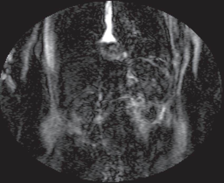
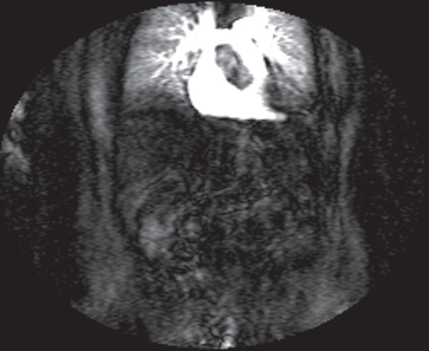
GCAs also undergo hepatic uptake, metabolism, and excretion into the biliary system. As such, they combine the properties of the extracellular agents and progressive enhancement of normal liver parenchyma with biliary excretion, which offers two main advantages for hepatic imaging: 1) delayed post-GCA imaging (usually 20 minutes) provides a homogeneously hyperintense background against which to detect hypointense non-hepatocellular lesions and 2) the possibility of detecting biliary ductal abnormalities, especially bile leaks through delayed GCA extravasation (usually after 20 minutes and as long as 45 minutes or longer). For most non-hepatobiliary indications, only extracellular GCAs are relevant. Although dynamic imaging—repetitive imaging of the same ROI before and repeatedly after gadolinium—plays a critical role and is customized to hepatic imaging, incorporating it into other body MRI protocols and interpretation schemes is straightforward. The duality of the hepatic blood supply necessitates dynamic imaging of the liver, but dynamic imaging offers utility elsewhere in the body and modern MR systems accomplish dynamic imaging without difficulty and the acquisition time penalty is minimal so dynamic imaging should be the default standard. Dynamic imaging relies on reproducible, rapid contrast delivery best achieved by power injecting (2–3 mL/sec). Timing the acquisition of the arterial phase images is critical and multiple techniques serve to gauge the arrival of contrast into the arterial system to accurately time the arterial phase of the examination (Fig. 1.17). The timing bolus is the time-tested and least technically intensive method. After an injection of a small volume of contrast (2–3 mL), a T1-weighted gradient-echo (GE) image is obtained at the level of the abdominal aorta until enhancement is detected—defining the onset of the arterial phase. The application of superior and inferior saturation pulses removes pseudoenhancement of the aorta and inferior vena cava (IVC), respectively, as a result of the inflow effect.
Real-time viewing of contrast transit (Bolus Track, Philips; CARE Bolus, Siemens; SmartPrep, GE; VisualPrep, Toshiba) involves careful monitoring by the technologist of serial large field-ofview (FOV) GE images after administration of the entire bolus of contrast (see Fig. 1.17). Transit of gadolinium through the superior vena cava (SVC) into the right heart through the pulmonary circulation and from the left heart into the aorta is portrayed on the monitor cinegraphically. With impending arrival of contrast into the abdominal aorta, the technologist instructs the patient to suspend respiration in preparation to acquire the arterial phase images. Portal phase images (or


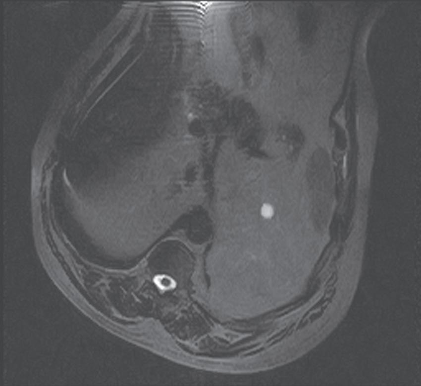
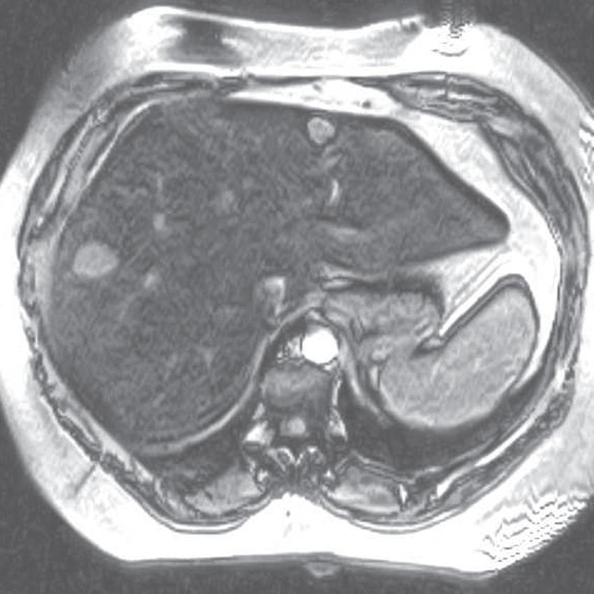
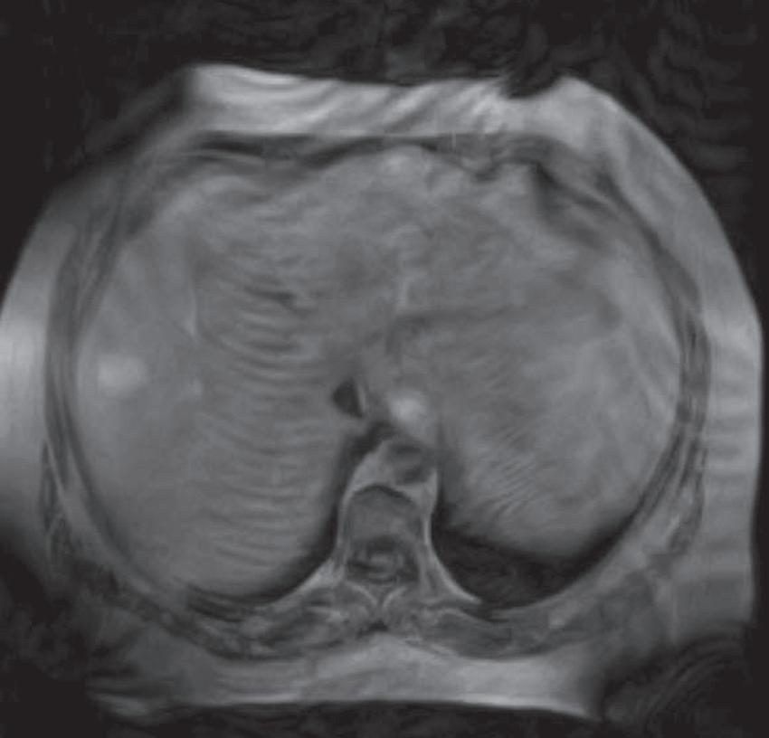
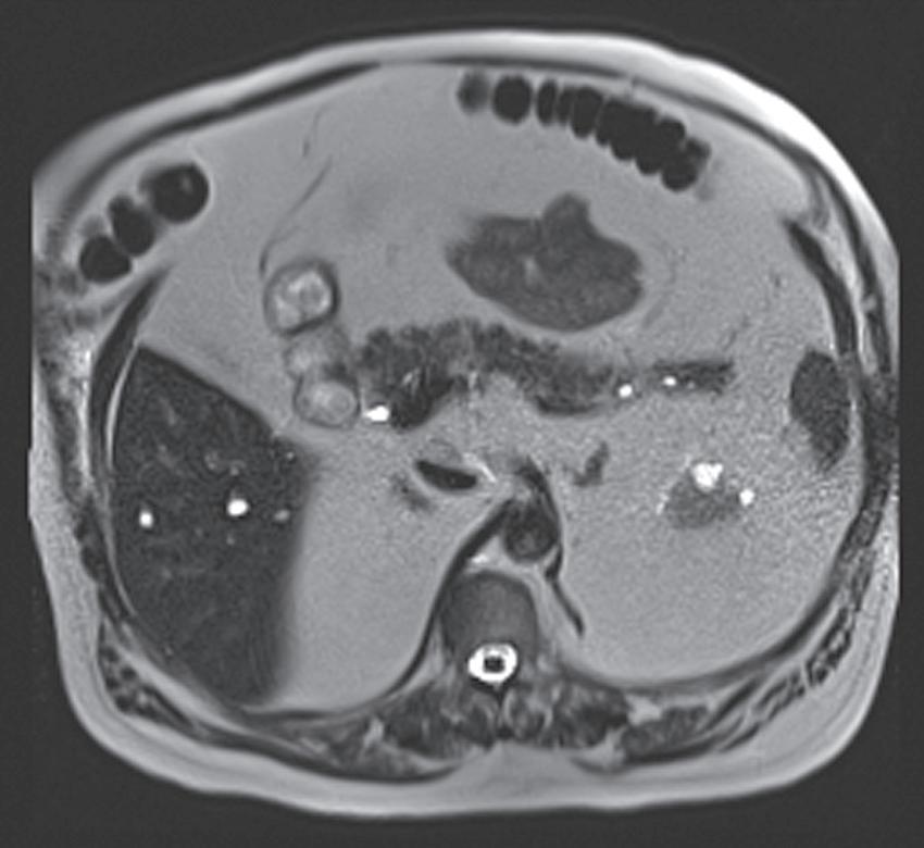
FIG. 1.15 Liver magnetic resonance imaging (MRI) obtained on a 0.3-Tesla system. Axial in-phase (A) and out-of-phase (B) images display relatively markedly diminished signal throughout the liver on the out-of-phase image compared with the in-phase image, indicating fatty infiltration. The axial T2-weighted image (C) reveals a small hyperintense lesion (arrow in C and D), which enhances as seen on the delayed T1-weighted gradient echo image (D), degraded by low signal-to-noise ratio and breathing motion artifact. Axial T2-weighted image obtained on a different patient on a 0.3-Tesla system (E) demonstrates prohibitive artifact distorting the image beyond diagnostic utility, compared with the corresponding image (F) from a follow-up study performed on a 1.5-Tesla short-bore, open-configuration system.
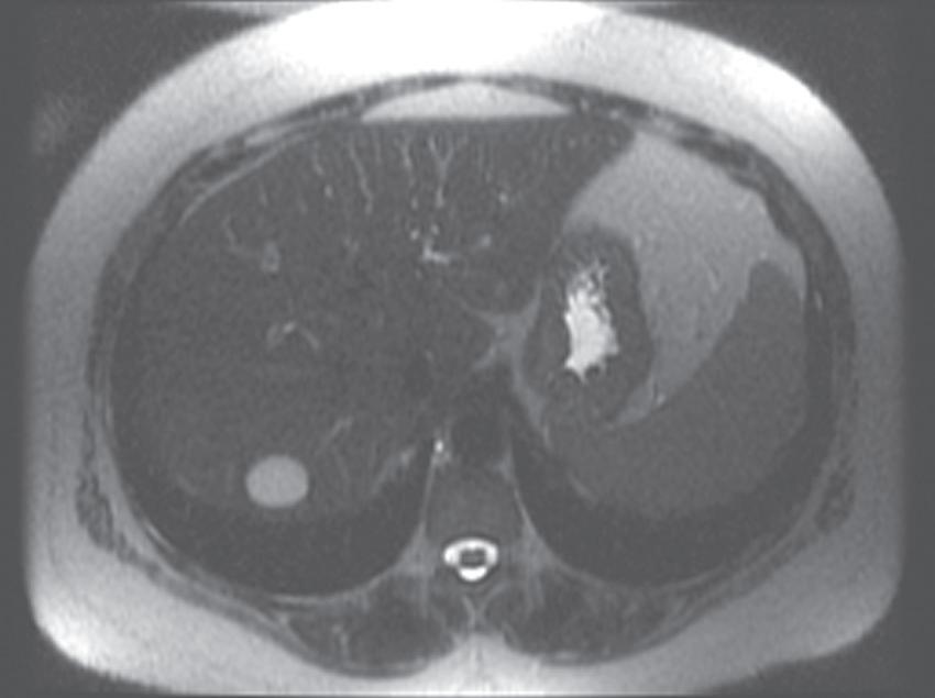

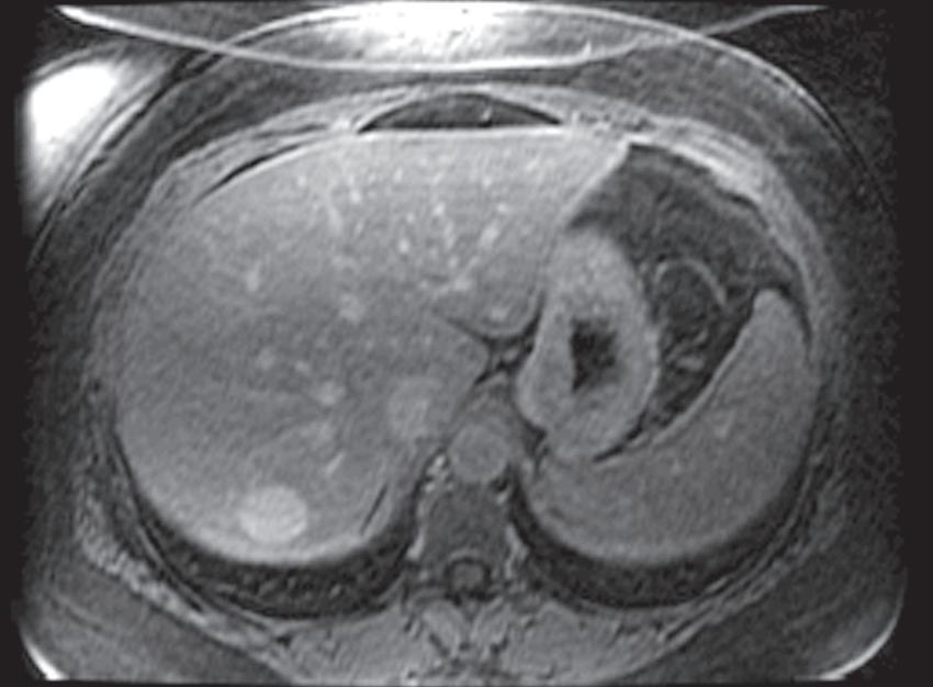

FIG. 1.16 Liver MRI obtained on a 1.5-Tesla system. In-phase (A) and out-of-phase (B) images demonstrate steatosis reflected by relative signal loss on the out-of-phase image. Axial T2-weighted single-shot fast spin-echo (SSFSE) image (C) reveals a small hyperintense lesion (arrow) in the posterior segment of the liver. The axial arterial (D) and delayed (E) images show initial clumped, peripheral, discontinuous enhancement with uniform, persistent enhancement (arrow). Note the higher signal-to-noise (SNR) and improved image quality compared with Fig. 1.15 A–D.
venous phase images, outside the liver) are subsequently obtained after allowing the patient to breathe after the arterial phase acquisition.
Practical demands prioritize throughput, necessitating economy of pulse sequences and mandating a rational approach to designing an MR protocol (Table 1.4). The following discussion generally applies to most abdominal and pelvic indications (selected niche applications—MR enterography,
MR urography, pelvic fistula, prostate, and other selected protocols include indication-specific modifications). Begin the examination with a large FOV (∼34 cm or larger) T2-weighted (single-shot fast spin-echo [SSFSE], GE; HASTE, Siemens; SSH-TSE, Philips; FASE, Toshiba; SSFSE, Hitachi) or steady-state sequence (balanced FFE, Philips; true-FISP, Siemens; True SSFP, Toshiba; FIESTA, GE). Each is a rapid sequence providing
TABLE 1.2 Gadolinium Formulations
MultiHance Gadobenic acid
Ablavar Gadofosveset trisodium Linear Ionic 91% kidney/9% bile
Eovist Gadoxetic acid disodium Linear Ionic 50% kidney/50% bile
ProHance Gadoteridol
Gadovist Gadobutrol
Gadoteric
Post liver transplant surveillance
Post chemoembolization or radioembolization
Liver lesion characterization (except FNH)
Abdominal or pelvic pain
Abdominal or pelvic mass
Tumor staging or followup
Female pelvis indications
Angiography (0.15 mmol/kg)
Enterography (0.1 mmol/kg)
Urography (0.07 mmol/kg)
Venography (0.15 mmol/kg)
Pelvic fistula (0.1 mmol/kg)
Higher relaxivity recommends use for these indications
Double plasma relaxivity, but not urine preempts signal loss from hyperconcentration
Prostate cancer workup Binds gadolinium less tightly than other extracellular agents and should be avoided in renal insufficiency
an anatomic overview. Assess proper coil placement—maximal signal should originate from the ROI—to the center of the abdomen. Needless to say, the entire ROI should be visible with adequate SNR (Fig. 1.18).
Thereafter, spatial resolution needs and acquisition time constraints determine FOV. Keeping the matrix constant (between 256 and 320 in the frequency axis), adapt the FOV to the patient’s size in order to maximize spatial resolution. Sacrifice visualization of the abdominal wall in order to boost spatial resolution, as long as wraparound artifact does not obscure the ROI (except when using parallel imaging where the wraparound artifact superimposes across the center of the image unless the FOV exceeds the ROI— discussed further in the Optimizing Body MRI section). Assign phase encoding to the anteroposterior (AP) axis and customize the phase FOV
Characterize FNH or differentiate from other liver lesions
Problem-solving diffuse liver disease (after extracellular agent)
Biliary abnormality (ie, bile leak)
Live liver donor transplant
Reduced hepatobiliary function limits enhancement
Less robust arterial enhancement
to the AP dimension of the patient because most patients are narrower in the AP dimension. Phase encoding costs time, according to the equation: acquisition time = TR × number of phase encoding steps × number of signal averages. Therefore decreasing phase-encoding FOV commensurate with patient size in the AP dimension saves time by eliminating phase-encoding steps (Fig. 1.19).
The standard protocol includes moderately and heavily T2-weighted, in- and out-ofphase GE, dynamic gadolinium-enhanced, and delayed postcontrast T1-weighted images (see Table 1.4). Add magnetic resonance cholangiopancreatography (MRCP) sequences if indicated. The SSFSE typically serves as the heavily T2-weighted sequence. Heavy T2-weighting means designing the sequence to favor signal from substances with long T2 values (eg, free unbound water—bile, urine, etc.). Sequence
TABLE 1.3 Contrast Agents
parameters include prolonged time to excitation (TE), usually between 180 and 200 msec, and time to repetition (TR) values. SSFSE sequences are obtained with a single excitation pulse followed by a rapid series of 180-degree pulses, each refocusing an echo until all of the k-space data for a single slice are acquired. So, technically, TR is nonexistent or infinite, because the excitation pulse is not repeated. Although relatively signal-starved (because of the single excitation pulse), the SSFSE sequence resists motion and susceptibility artifact (Fig. 1.20). The rapid acquisition protects against motion artifact and the multiple refocusing pulses repeatedly undo, or correct for, susceptibility artifact. Heavy T2-weighting optimizes tissue contrast for visualizing fluid-filled structures, such as the gallbladder and biliary tree—sort of a “poor man’s MRCP.”
In- and out-of-phase images are T1-weighted GE images with TE values timed to coincide
with fat and water molecules precessing in-phase and out-of-phase, respectively. On most scanners, these images are obtained simultaneously as a double-echo sequence in a single breathhold; at each slice, one image with an in-phase TE and one image with an out-of-phase TE are obtained concurrently. TE values are fixed by magnetic field strength according to the Larmor equation (Table 1.5). These images provide T1-weighting and the ability to detect fat deposition (among other things, which are discussed in the forthcoming section).
The examination revolves around the dynamic gadolinium-enhanced sequence. Dynamic refers to the temporal sense of the word—obtaining views at the same location repetitively after contrast. Since gadolinium is a T1-shortening agent, detection of gadolinium enhancement necessitates a T1-weighted sequence. Improved dynamic range afforded by fat suppression further improves enhancement conspicuity. High spatial
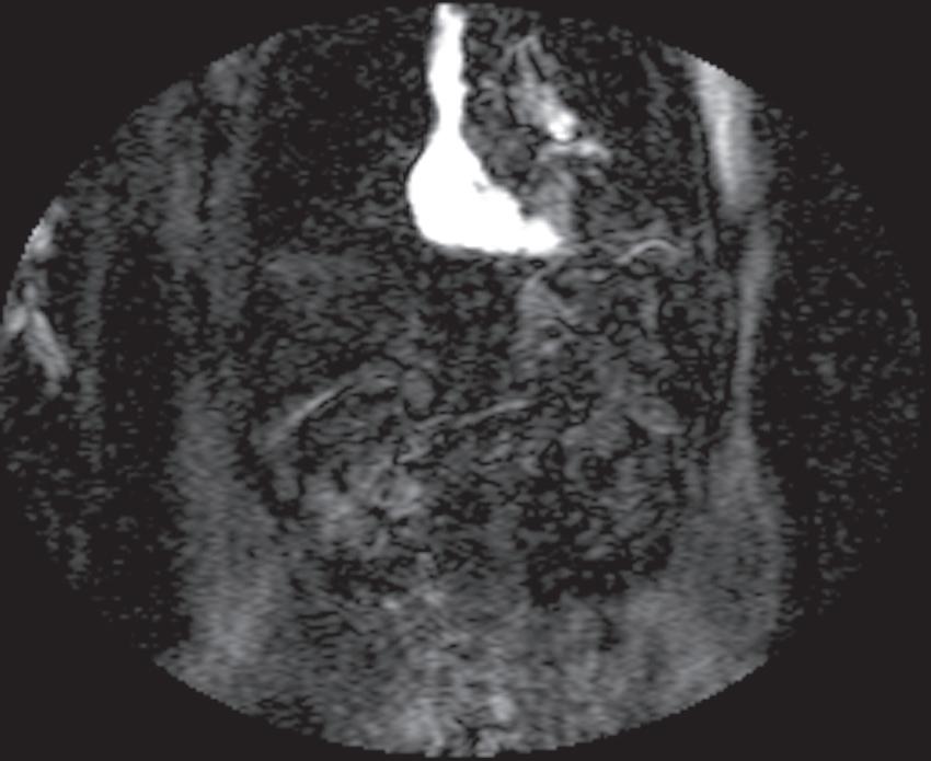
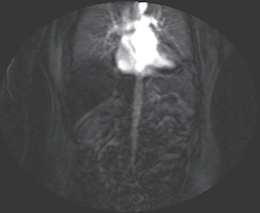
FIG. 1.17 Example of Bolus Track timing sequence to initiate the dynamic acquisition. Selected serial coronal large field-of-view gradient-echo images obtained immediately after the intravenous administration of gadolinium (A–D) reveal the inflow of gadolinium into the superior vena cava (SVC; A), the right ventricle (B), through the pulmonary outflow tract and into the pulmonary arterial system (C), and into the thoracic aorta, down the abdominal aorta (D).
TABLE 1.4 Sample Abdominal Protocol
Steady-state 3-plane, axial or coronal
Heavily T2weighted
T2/T1-weighted; balanced gradients in all axes ➔ insensitive to motion
Usually performed with single-shot technique
dependent on magnetic field strength; unnecessary with dynamic Dixon sequence Dynamic Axial 3-D Min/min 4–5 (interpolated to 2–2.5)
Ideally with fat suppression or Dixon technique; precontrast, arterial and portal phases
Moderately T2weighted
Delayed postcontrast Axial 2-D or 3-D Min/min 2-D: 5 × 0 3D: same as dynamic
2-D MRCP Radial 2-D NA/600–1000 40
Diffusion (b = 20) Axial 2-D Min/min 8 × 1
Diffusion (b = 800) Axial 2-D Min/min 8 × 1
Hepatobiliary Axial 3-D Min/min 4–5 (interpolated to 2–2.5)
Ideally with fat suppression
Ideally with fat suppression
Centered on CBD
Respiratory-triggered
T2-weighted + perfusionweighted + diffusionweighted
T2-weighted + diffusionweighted
Same as dynamic sequence except increased flip angle (30 degrees optimally)
FIG. 1.18 Assessing coil placement. (A) Coronal localizing SSFSE T2-weighted image reveals maximal signal emanating from the lower abdomen, instead of the upper. (B) Coronal localizing SSFSE T2-weighted image of a different patient reveals a mildly hyperintense exophytic lesion (arrow) arising from the lateral segment of the liver, which is well visualized because of optimal coil placement, yielding superior signal over the region of interest.
synchronized with the arrival of gadolinium in the arterial system (as previously discussed), constitutes the arterial phase images. Following a short delay to allow the patient to breathe (more relevant for the abdomen), a third set of images with the same parameters is acquired, serving as the portal phase images of the abdomen.
Deferring delayed enhanced images until after acquiring the moderately T2-weighted images achieves a reasonable delay. Moderately T2-weighted images possess better tissue contrast compared with their heavily T2-weighed counterparts and the presence of intravenous gadolinium confers even higher conspicuity for solid liver lesions, compared with normal parenchyma.12 Normal tissue retains more gadolinium and the associated magnetization transfer effects diminish parenchymal signal, resulting in a greater lesion-to-liver contrast-to-noise ratio (CNR). Fat suppression conveys greater tissue contrast by improving dynamic range. Moderate T2-weighting requires TE values on the order of 80 msec and the fast spin-echo (FSE)—or turbo spin-echo (TSE)—sequence adapts best to this parameter requirement within the constraints of a breathhold. Whereas the FSE sequence
rapidly fills k space, enabling breathhold imaging, the relatively longer acquisition time compared with other sequences (such as the SSFSE), especially on older systems, challenges breathholding. Respiratory triggering circumvents this problem.
The delayed (or interstitial or equilibrium) phase images depict the eventual passage of contrast into the extravascular space, perfusing the interstitial tissues. Either 3-D or 2-D T1-weighted fat-suppressed GE sequences suffice. Three-dimensional pulse sequences potentially suffer more from breathing motion artifact—obviated on the 2-D sequence, when fragmented into multiple breathholds.
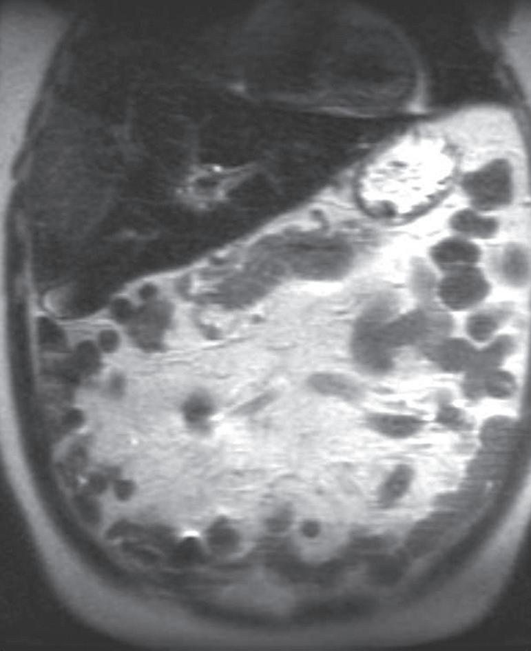
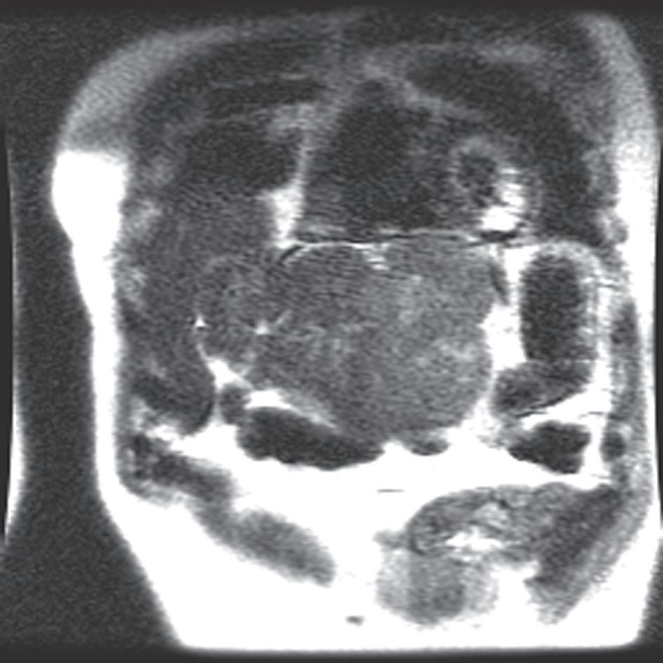
The “interstitial” designation on delayed postcontrast images only applies with the use of extracellular GCAs. When a combination agent is used, the delayed postcontrast images are referred to as “hepatobiliary” phase images because the vast majority of the contrast inhabits the liver parenchyma and subsequently experiences biliary excretion (Fig. 1.21).
PULSE SEQUENCES
The process of filling k space depends on the pulse sequence chosen. Two major types of pulse sequences dominate body MRI (and MRI in general): 1) SE and 2) GE. The presence or absence of a “refocusing pulse” characterizes the SE and GE sequences, respectively. These two pulse sequences represent different approaches to the problem of generating a signal after the initial Rf excitation pulse. The frequency-encoding gradient dephases the excited spins (ie, destructive interference), which must be rephased in order to yield signal—referred to as an echo of the original Rf excitation pulse, reverberating at

FIG. 1.21 Axial hepatobiliary phase image (A) in a patient with ocular melanoma showing excreted contrast in the hepatic ducts (arrows) and a hypointense metastasis in segment two (thick arrow), rendered very conspicuously against the hyperintense background of the normal liver parenchyma. Axial hepatobiliary phase image more caudally (B) demonstrates renal contrast excretion and excreted contrast in the gallbladder and common bile duct (arrow)