THOMAS’ CALCULUS
FOURTEENTH EDITION IN SI UNITS
Based on the original work by GEORGE B. THOMAS, JR.
Massachusetts Institute of Technology as revised by
JOEL HASS
University of California, Davis
CHRISTOPHER HEIL
Georgia Institute of Technology
MAURICE D. WEIR
Naval Postgraduate School
SI conversion by JOSÉ LUIS ZULETA ESTRUGO
École Polytechnique Fédérale de Lausanne
Director, Portfolio Management: Deirdre Lynch
Executive Editor: Jeff Weidenaar
Editorial Assistant: Jennifer Snyder
Content Producer: Rachel S. Reeve
Managing Producer: Scott Disanno
Producer: Stephanie Green
TestGen Content Manager: Mary Durnwald
Manager: Content Development, Math: Kristina Evans
Product Marketing Manager: Emily Ockay
Field Marketing Manager: Evan St. Cyr
Marketing Assistants: Jennifer Myers, Erin Rush
Senior Author Support/Technology Specialist: Joe Vetere
Rights and Permissions Project Manager: Gina M. Cheselka
Manufacturing Buyer: Carol Melville, LSC Communications, Inc.
Program Design Lead: Barbara T. Atkinson
Associate Director of Design: Blair Brown
Senior Manufacturing Controller, Global Edition: Caterina Pellegrino
Editor, Global Edition: Subhasree Patra
Production Coordination, Composition: Pearson CSC
Cover Design: Lumina Datamatics Ltd.
Illustrations: Network Graphics, Cenveo® Publisher Services
Cover Image: Brian Kenney/Shutterstock
Attributions of third party content appear on page C-1, which constitutes an extension of this copyright page. PEARSON, ALWAYS LEARNING, and MYLAB MATH are exclusive trademarks owned by Pearson Education, Inc. or its affiliates in the U.S. and/or other countries.
Pearson Education Limited
KAO Two
KAO Park Harlow CM17 9NA United Kingdom
and Associated Companies throughout the world
Visit us on the World Wide Web at: www.pearsonglobaleditions.com
© Pearson Education Limited, 2020
The rights of Joel Hass, Christopher Heil, and Maurice Weir to be identified as the authors of this work have been asserted by them in accordance with the Copyright, Designs and Patents Act 1988.
Authorized adaptation from the United States edition, entitled Thomas’ Calculus, 14th Edition, ISBN 978-0-13-443898-6 by Joel Hass, Christopher Heil, and Maurice Weir, published by Pearson Education, Inc., © 2018, 2014, 2010
All rights reserved. No part of this publication may be reproduced, stored in a retrieval system, or transmitted in any form or by any means, electronic, mechanical, photocopying, recording or otherwise, without either the prior written permission of the publisher or a license permitting restricted copying in the United Kingdom issued by the Copyright Licensing Agency Ltd, Saffron House, 6–10 Kirby Street, London EC1N 8TS.
All trademarks used herein are the property of their respective owners. The use of any trademark in this text does not vest in the author or publisher any trademark ownership rights in such trademarks, nor does the use of such trademarks imply any affiliation with or endorsement of this book by such owners. For information regarding permissions, request forms, and the appropriate contacts within the Pearson Education Global Rights and Permissions department, please visit www.pearsoned.com/permissions.
This eBook is a standalone product and may or may not include all assets that were part of the print version. It also does not provide access to other Pearson digital products like MyLab and Mastering. The publisher reserves the right to remove any material in this eBook at any time.
British Library Cataloguing-in-Publication Data
A catalogue record for this book is available from the British Library
ISBN 10: 1-292-25322-3
ISBN 13: 978-1-292-25322-0
eBook ISBN 13: 978-1-292-25329-9
Typeset by Integra Software Services.
Preface 9
1 Functions 19
1.1 Functions and Their Graphs 19
1.2 Combining Functions; Shifting and Scaling Graphs 32
1.3 Trigonometric Functions 39
1.4 Graphing with Software 47
Questions to Guide Your Review 51
Practice Exercises 52
Additional and Advanced Exercises 53
Technology Application Projects 55
2
3
Limits and Continuity 56
2.1 Rates of Change and Tangent Lines to Curves 56
2.2 Limit of a Function and Limit Laws 63
2.3 The Precise Definition of a Limit 74
2.4 One-Sided Limits 83
2.5 Continuity 90
2.6 Limits Involving Infinity; Asymptotes of Graphs 101
Questions to Guide Your Review 114
Practice Exercises 115
Additional and Advanced Exercises 116
Technology Application Projects 119
Derivatives 120
3.1 Tangent Lines and the Derivative at a Point 120
3.2 The Derivative as a Function 124
3.3 Differentiation Rules 133
3.4 The Derivative as a Rate of Change 142
3.5 Derivatives of Trigonometric Functions 152
3.6 The Chain Rule 158
3.7 Implicit Differentiation 166
3.8 Related Rates 171
3.9 Linearization and Differentials 180
Questions to Guide Your Review 192
Practice Exercises 192
Additional and Advanced Exercises 197
Technology Application Projects 200
4
Applications of Derivatives 201
4.1 Extreme Values of Functions on Closed Intervals 201
4.2 The Mean Value Theorem 209
4.3 Monotonic Functions and the First Derivative Test 215
4.4 Concavity and Curve Sketching 220
4.5 Applied Optimization 232
4.6 Newton’s Method 244
4.7 Antiderivatives 249
Questions to Guide Your Review 259
Practice Exercises 259
Additional and Advanced Exercises 262
Technology Application Projects 265
5
Integrals 266
5.1 Area and Estimating with Finite Sums 266
5.2 Sigma Notation and Limits of Finite Sums 276
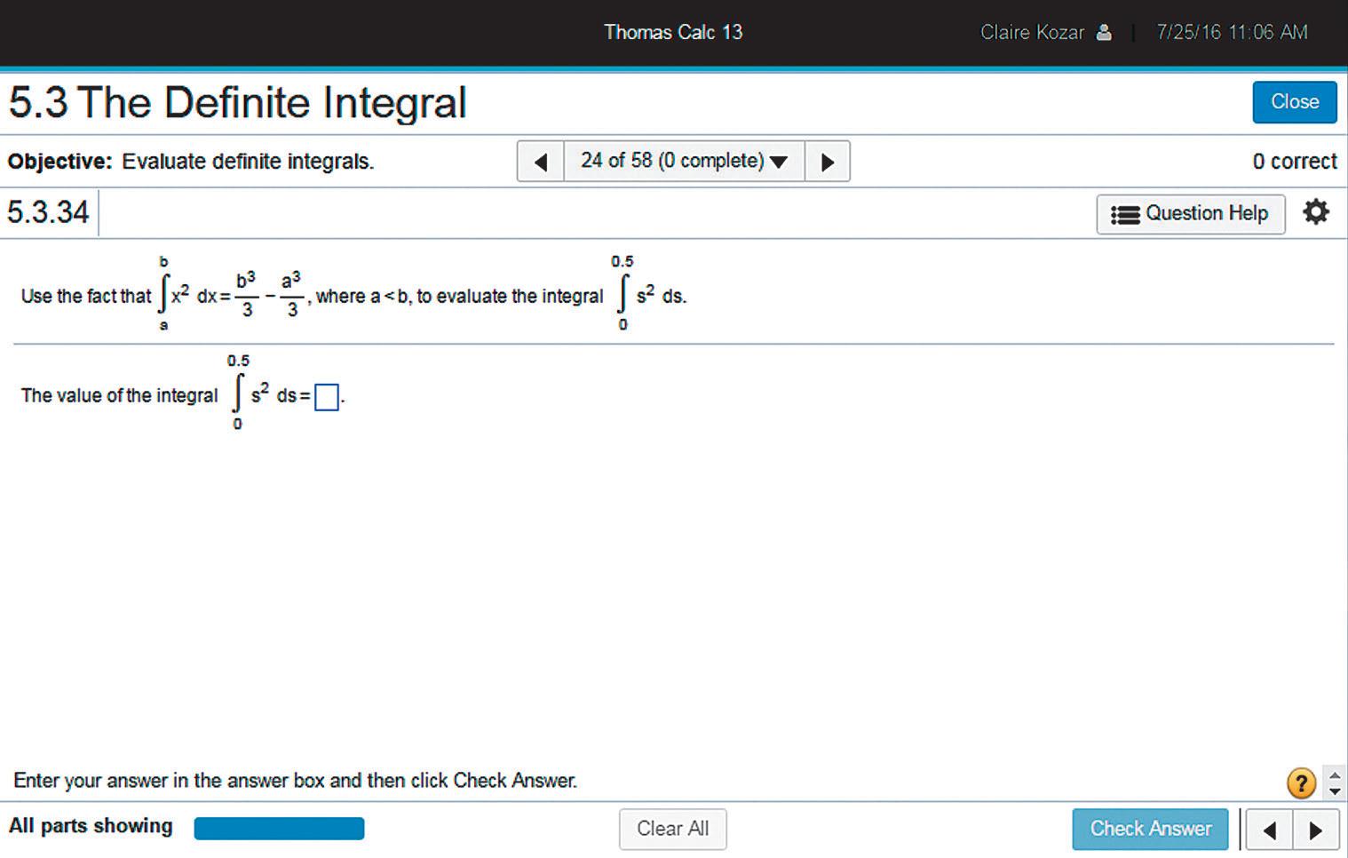
5.3 The Definite Integral 283
5.4 The Fundamental Theorem of Calculus 296
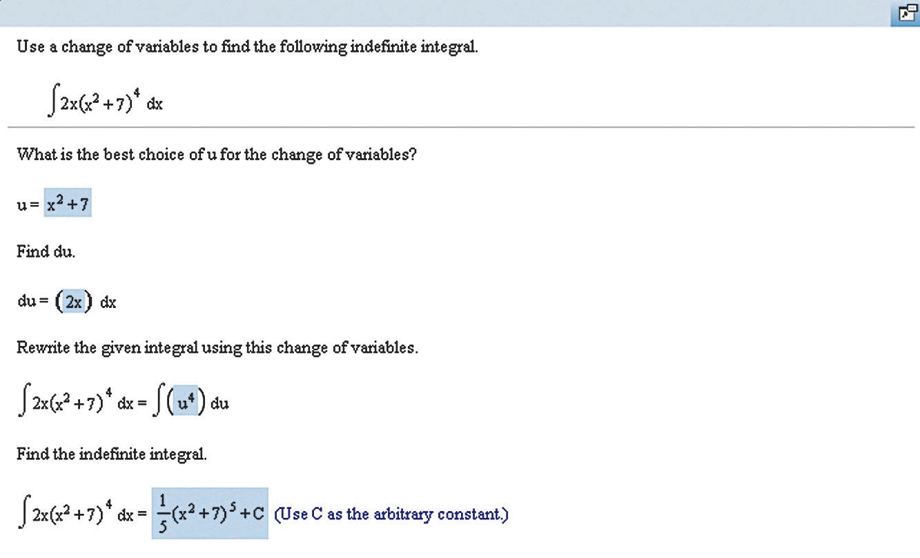
5.5 Indefinite Integrals and the Substitution Method 307
5.6 Definite Integral Substitutions and the Area Between Curves 314 Questions to Guide Your Review 324
Practice Exercises 325
Additional and Advanced Exercises 328
Technology Application Projects 331
6
Applications of Definite Integrals 332
6.1 Volumes Using Cross-Sections 332
6.2 Volumes Using Cylindrical Shells 343
6.3 Arc Length 351
6.4 Areas of Surfaces of Revolution 356
6.5 Work and Fluid Forces 362
6.6 Moments and Centers of Mass 371 Questions to Guide Your Review 383 Practice Exercises 384
Additional and Advanced Exercises 386 Technology Application Projects 387
7
Transcendental Functions 388
7.1 Inverse Functions and Their Derivatives 388
7.2 Natural Logarithms 396
7.3 Exponential Functions 404
7.4 Exponential Change and Separable Differential Equations 415
7.5 Indeterminate Forms and L’Hôpital’s Rule 425
7.6 Inverse Trigonometric Functions 434
7.7 Hyperbolic Functions 446
7.8 Relative Rates of Growth 454
Questions to Guide Your Review 459
Practice Exercises 460
Additional and Advanced Exercises 463
8 Techniques of Integration 465
8.1 Using Basic Integration Formulas 465
8.2 Integration by Parts 470
8.3 Trigonometric Integrals 478
8.4 Trigonometric Substitutions 484
8.5 Integration of Rational Functions by Partial Fractions 489
8.6 Integral Tables and Computer Algebra Systems 497
8.7 Numerical Integration 503
8.8 Improper Integrals 512
Questions to Guide Your Review 523
Practice Exercises 524
Additional and Advanced Exercises 526
Technology Application Projects 529
9
Infinite Sequences and Series 530
9.1 Sequences 530
9.2 Infinite Series 543
9.3 The Integral Test 553
9.4 Comparison Tests 559
9.5 Absolute Convergence; The Ratio and Root Tests 564
9.6 Alternating Series and Conditional Convergence 571
9.7 Power Series 578
9.8 Taylor and Maclaurin Series 589
9.9 Convergence of Taylor Series 594
9.10 Applications of Taylor Series 601
Questions to Guide Your Review 610
Practice Exercises 611
Additional and Advanced Exercises 613
Technology Application Projects 615
10
Parametric Equations and Polar Coordinates 616
10.1 Parametrizations of Plane Curves 616
10.2 Calculus with Parametric Curves 625
10.3 Polar Coordinates 634
10.4 Graphing Polar Coordinate Equations 638
10.5 Areas and Lengths in Polar Coordinates 642
10.6 Conic Sections 647
10.7 Conics in Polar Coordinates 655
Questions to Guide Your Review 661
Practice Exercises 662
Additional and Advanced Exercises 664
Technology Application Projects 666
11
Vectors and the Geometry of Space 667
11.1 Three-Dimensional Coordinate Systems 667
11.2 Vectors 672
11.3 The Dot Product 681
11.4 The Cross Product 689
11.5 Lines and Planes in Space 695
11.6 Cylinders and Quadric Surfaces 704
Questions to Guide Your Review 710 Practice Exercises 710
Additional and Advanced Exercises 712
Technology Application Projects 715
12
Vector-Valued Functions and Motion in Space 716
12.1 Curves in Space and Their Tangents 716
12.2 Integrals of Vector Functions; Projectile Motion 725
12.3 Arc Length in Space 734
12.4 Curvature and Normal Vectors of a Curve 738
12.5 Tangential and Normal Components of Acceleration 744
12.6 Velocity and Acceleration in Polar Coordinates 750
Questions to Guide Your Review 754
Practice Exercises 755
Additional and Advanced Exercises 757
Technology Application Projects 758
13
Partial Derivatives 759
13.1 Functions of Several Variables 759
13.2 Limits and Continuity in Higher Dimensions 767
13.3 Partial Derivatives 776
13.4 The Chain Rule 788
13.5 Directional Derivatives and Gradient Vectors 798
13.6 Tangent Planes and Differentials 806
13.7 Extreme Values and Saddle Points 816
13.8 Lagrange Multipliers 825
13.9 Taylor’s Formula for Two Variables 835
13.10 Partial Derivatives with Constrained Variables 839
Questions to Guide Your Review 843
Practice Exercises 844
Additional and Advanced Exercises 847
Technology Application Projects 849
14
Multiple Integrals 850
14.1 Double and Iterated Integrals over Rectangles 850
14.2 Double Integrals over General Regions 855
14.3 Area by Double Integration 864
14.4 Double Integrals in Polar Form 867
14.5 Triple Integrals in Rectangular Coordinates 874
14.6 Applications 884
14.7 Triple Integrals in Cylindrical and Spherical Coordinates 894
14.8
Substitutions in Multiple Integrals 906
Questions to Guide Your Review 916
Practice Exercises 916
Additional and Advanced Exercises 919
Technology Application Projects 921
15
Integrals and Vector Fields 922
15.1 Line Integrals of Scalar Functions 922
15.2 Vector Fields and Line Integrals: Work, Circulation, and Flux 929
15.3 Path Independence, Conservative Fields, and Potential Functions 942
15.4 Green’s Theorem in the Plane 953
15.5 Surfaces and Area 965
15.6 Surface Integrals 975
15.7 Stokes’ Theorem 985
15.8 The Divergence Theorem and a Unified Theory 998
Questions to Guide Your Review 1011
Practice Exercises 1011
Additional and Advanced Exercises 1014
Technology Application Projects 1015
16
First-Order Differential Equations 1016
16.1 Solutions, Slope Fields, and Euler’s Method 1016
16.2 First-Order Linear Equations 1024
16.3 Applications 1030
16.4 Graphical Solutions of Autonomous Equations 1036
16.5 Systems of Equations and Phase Planes 1043
Questions to Guide Your Review 1049
Practice Exercises 1049
Additional and Advanced Exercises 1051
Technology Application Projects 1052
Second-Order
Differential Equations (Online)
17.1 Second-Order Linear Equations
17.2 Nonhomogeneous Linear Equations
17.3 Applications
17.4 Euler Equations
17.5 Power-Series Solutions
Appendices AP-1
A.1 Real Numbers and the Real Line AP-1
A.2 Mathematical Induction AP-6
A.3 Lines, Circles, and Parabolas AP-9
A.4 Proofs of Limit Theorems AP-19
A.5 Commonly Occurring Limits AP-22
A.6 Theory of the Real Numbers AP-23
A.7 Complex Numbers AP-26
A.8 Probability AP-34
A.9 The Distributive Law for Vector Cross Products AP-47
A.10 The Mixed Derivative Theorem and the Increment Theorem AP-49
Answers to Odd-Numbered Exercises A-1
Credits C-1
Applications Index AI-1
Preface
Thomas’ Calculus, Fourteenth Edition in SI Units, provides a modern introduction to calculus that focuses on developing conceptual understanding of the underlying mathematical ideas. This text supports a calculus sequence typically taken by students in STEM fields over several semesters. Intuitive and precise explanations, thoughtfully chosen examples, superior figures, and time-tested exercise sets are the foundation of this text. We continue to improve this text in keeping with shifts in both the preparation and the goals of today’s students, and in the applications of calculus to a changing world.
Many of today’s students have been exposed to calculus in high school. For some, this translates into a successful experience with calculus in college. For others, however, the result is an overconfidence in their computational abilities coupled with underlying gaps in algebra and trigonometry mastery, as well as poor conceptual understanding. In this text, we seek to meet the needs of the increasingly varied population in the calculus sequence. We have taken care to provide enough review material (in the text and appendices), detailed solutions, and a variety of examples and exercises, to support a complete understanding of calculus for students at varying levels. Within the text, we present the material in a way that supports the development of mathematical maturity, going beyond memorizing formulas and routine procedures, and we show students how to generalize key concepts once they are introduced. References are made throughout, tying new concepts to related ones that were studied earlier. After studying calculus from Thomas, students will have developed problem-solving and reasoning abilities that will serve them well in many important aspects of their lives. Mastering this beautiful and creative subject, with its many practical applications across so many fields, is its own reward. But the real gifts of studying calculus are acquiring the ability to think logically and precisely; understanding what is defined, what is assumed, and what is deduced; and learning how to generalize conceptually. We intend this book to encourage and support those goals. New to This Edition
We welcome to this edition a new coauthor, Christopher Heil from the Georgia Institute of Technology. He has been involved in teaching calculus, linear algebra, analysis, and abstract algebra at Georgia Tech since 1993. He is an experienced author and served as a consultant on the previous edition of this text. His research is in harmonic analysis, including time-frequency analysis, wavelets, and operator theory.
This is a substantial revision. Every word, symbol, and figure was revisited to ensure clarity, consistency, and conciseness. Additionally, we made the following text-wide updates:
• Updated graphics to bring out clear visualization and mathematical correctness.
• Added examples (in response to user feedback) to overcome conceptual obstacles. See Example 3 in Section 16.1
• Added new types of homework exercises throughout, including many with a geometric nature. The new exercises are not just more of the same, but rather give different perspectives on and approaches to each topic. We also analyzed aggregated student usage and performance data from MyLab Math for the previous edition of this text. The results of this analysis helped improve the quality and quantity of the exercises.
• Added short URLs to historical links that allow students to navigate directly to online information.
• Added new marginal notes throughout to guide the reader through the process of problem solution and to emphasize that each step in a mathematical argument is rigorously justified.
New to MyLab Math®
Many improvements have been made to the overall functionality of MyLab Math since the previous edition. Beyond that, we have also increased and improved the content specific to this text.
• Instructors now have more exercises than ever to choose from in assigning homework.
• The MyLab Math exercise-scoring engine has been updated to allow for more robust coverage of certain topics, including differential equations.
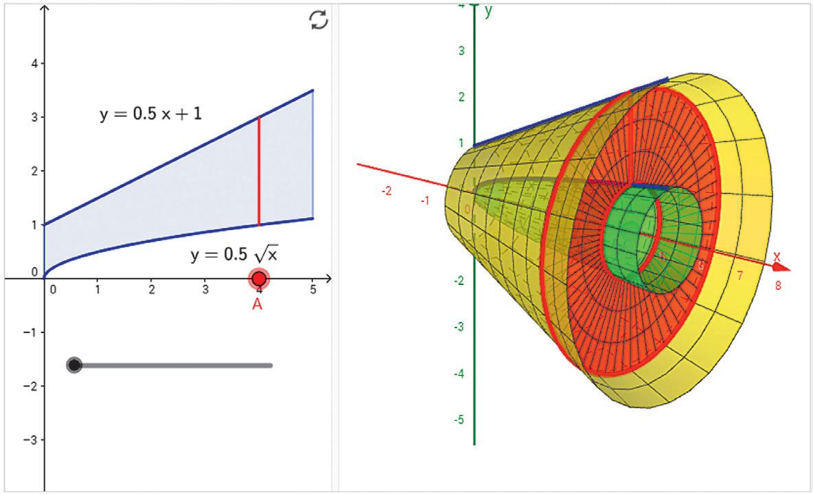
• A full suite of Interactive Figures have been added to support teaching and learning. The figures are designed to be used in lecture, as well as by students independently. The figures are editable using the freely available GeoGebra software. The figures were created by Marc Renault (Shippensburg University), Kevin Hopkins (Southwest Baptist University), Steve Phelps (University of Cincinnati), and Tim Brzezinski (Berlin High School, CT).
• Enhanced Sample Assignments include just-in-time prerequisite review, help keep skills fresh with distributed practice of key concepts (based on research by Jeff Hieb of University of Louisville), and provide opportunities to work exercises without learning aids (to help students develop confidence in their ability to solve problems independently).
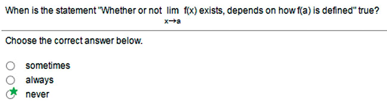
• Additional Conceptual Questions augment text exercises to focus on deeper, theoretical understanding of the key concepts in calculus. These questions were written by faculty at Cornell University under an NSF grant. They are also assignable through Learning Catalytics.
• Setup & Solve exercises now appear in many sections. These exercises require students to show how they set up a problem as well as the solution, better mirroring what is required of students on tests.
• New instructional videos by Greg Wisloski and Dan Radelet (both of Indiana University of PA) augment the already robust collection within the course. These videos support the overall approach of the text—specifically, they go beyond routine procedures to show students how to generalize and connect key concepts.
Content Enhancements
Chapter 1
• Shortened 1.4 to focus on issues arising in use of mathematical software and potential pitfalls. Removed peripheral material on regression, along with associated exercises.
• Added new Exercises: 1.1: 59–62, 1.2: 21–22; 1.3: 64–65, PE: 29–32.
Chapter 2
• Added definition of average speed in 2.1.
• Clarified definition of limits to allow for arbitrary domains. The definition of limits is now consistent with the definition in multivariable domains later in the text and with more general mathematical usage.
• Reworded limit and continuity definitions to remove implication symbols and improve comprehension.
• Added new Example 7 in 2.4 to illustrate limits of ratios of trig functions.
• Rewrote 2.5 Example 11 to solve the equation by finding a zero, consistent with previous discussion.
• Added new Exercises: 2.1: 15–18; 2.2: 3h–k, 4f–i; 2.4: 19–20, 45–46; 2.6: 69–72; PE: 49–50; AAE: 33.
Chapter 3
• Clarified relation of slope and rate of change.
• Added new Figure 3.9 using the square root function to illustrate vertical tangent lines.
• Added figure of x sin (1 > x) in 3 2 to illustrate how oscillation can lead to nonexistence of a derivative of a continuous function.
• Revised product rule to make order of factors consistent throughout text, including later dot product and cross product formulas.
• Added new Exercises: 3.2: 36, 43–44; 3.3: 51–52; 3.5: 43–44, 61bc; 3.6: 65–66, 97–99; 3.7: 25–26; 3.8: 47; AAE: 24–25.
Chapter 4
• Added summary to 4.1.
• Added new Example 3 with new Figure 4.27 to give basic and advanced examples of concavity.
• Added new Exercises: 4.1: 61–62; 4.3: 61–62; 4.4: 49–50, 99–104; 4.5: 37–40; 4.6: 7–8; 4.7: 93–96; PE: 1–10; AAE: 19–20, 33. Moved Exercises 4.1: 53–68 to PE.
Chapter 5
• Improved discussion in 5.4 and added new Figure 5.18 to illustrate the Mean Value Theorem.
• Added new Exercises: 5.2: 33–36; PE: 45–46.
Chapter 6
• Clarified cylindrical shell method.
• Added introductory discussion of mass distribution along a line, with figure, in 6.6.
• Added new Exercises: 6.1: 15–16; 6.2: 45–46; 6.5: 1–2; 6.6: 1–6, 19–20; PE: 17–18, 35–36.
Chapter 7
• Added explanation for the terminology “indeterminate form.”
• Clarified discussion of separable differential equations in 7.4.
• Replaced sin- 1 notation for the inverse sine function with arcsin as default notation in 7.6, and similarly for other trig functions.
• Added new Exercises: 7.2: 5–6, 75–76; 7.3: 5–6, 31–32, 123–128, 149–150; 7.6: 43–46, 95–96; AAE: 9–10, 23.
Chapter 8
• Updated 8.2 Integration by Parts discussion to emphasize u(x)v (x) dx form rather than u dv. Rewrote Examples 1–3 accordingly.
• Removed discussion of tabular integration and associated exercises.
• Updated discussion in 8.5 on how to find constants in Partial Fraction method.
• Updated notation in 8.8 to align with standard usage in statistics.
• Added new Exercises: 8.1: 41–44; 8.2: 53–56, 72–73; 8.3: 75–76; 8.4: 49–52; 8.5: 51–66, 73–74; 8.8: 35–38, 77–78; PE: 69–88.
Chapter 9
• Clarified the different meaning of a sequence and a series.
• Added new Figure 9.9 to illustrate sum of a series as area of a histogram.
• Added to 9.3 a discussion on the importance of bounding errors in approximations.
• Added new Figure 9.13 illustrating how to use integrals to bound remainder terms of partial sums.
• Rewrote Theorem 10 in 9.4 to bring out similarity to the integral comparison test.
• Added new Figure 9.16 to illustrate the differing behaviors of the harmonic and alternating harmonic series.
• Renamed the nth term test the “nth term test for divergence” to emphasize that it says nothing about convergence.
• Added new Figure 9.19 to illustrate polynomials converging to ln (1 + x) , which illustrates convergence on the half-open interval (- 1, 1] .
• Used red dots and intervals to indicate intervals and points where divergence occurs and blue to indicate convergence throughout Chapter 9.
• Added new Figure 9.21 to show the six different possibilities for an interval of convergence.
• Added new Exercises: 9.1: 27–30, 72–77; 9.2: 19–22, 73–76, 105; 9.3: 11–12, 39–42; 9.4: 55–56; 9.5: 45–46, 65–66; 9.6: 57–82; 9.7: 61–65; 9.8: 23–24, 39–40; 9.9: 11–12, 37–38; PE: 41–44, 97–102.
Chapter 10
• Added new Example 1 and Figure 10.2 in 10.1 to give a straightforward first example of a parametrized curve.
• Updated area formulas for polar coordinates to include conditions for positive r and non-overlapping u
• Added new Example 3 and Figure 10.37 in 10.4 to illustrate intersections of polar curves.
• Added new Exercises: 10.1: 19–28; 10.2: 49–50; 10.4: 21–24.
Chapter 11
• Added new Figure 11.13(b) to show the effect of scaling a vector.
• Added new Example 7 and Figure 11.26 in 11.3 to illustrate projection of a vector.
• Added discussion on general quadric surfaces in 11.6, with new Example 4 and new Figure 11.48 illustrating the description of an ellipsoid not centered at the origin via completing the square.
• Added new Exercises: 11.1: 31–34, 59–60, 73–76; 11.2: 43–44; 11.3: 17–18; 11.4: 51–57; 11.5: 49–52.
Chapter 12
• Added sidebars on how to pronounce Greek letters such as kappa, tau, etc.
• Added new Exercises: 12.1: 1–4, 27–36; 12.2: 15–16, 19–20; 12.4: 27–28; 12.6: 1–2.
Chapter 13
• Elaborated on discussion of open and closed regions in 13.1.
• Standardized notation for evaluating partial derivatives, gradients, and directional derivatives at a point, throughout the chapter.
• Renamed “branch diagrams” as “dependency diagrams” which clarifies that they capture dependence of variables.
• Added new Exercises: 13.2: 51–54; 13.3: 51–54, 59–60, 71–74, 103–104; 13.4: 20–30, 43–46, 57–58; 13.5: 41–44; 13.6: 9–10, 61; 13.7: 61–62.
Chapter 14
• Added new Figure 14.21b to illustrate setting up limits of a double integral.
• Added new 14.5 Example 1, modified Examples 2 and 3, and added new Figures 14.31, 14.32, and 14.33 to give basic examples of setting up limits of integration for a triple integral.
• Added new material on joint probability distributions as an application of multivariable integration.
• Added new Examples 5, 6 and 7 to Section 14.6.
• Added new Exercises: 14.1: 15–16, 27–28; 14.6: 39–44; 14.7: 1–22.
Chapter 15
• Added new Figure 15.4 to illustrate a line integral of a function.
• Added new Figure 15.17 to illustrate a gradient field.
• Added new Figure 15.19 to illustrate a line integral of a vector field.
• Clarified notation for line integrals in 15.2.
• Added discussion of the sign of potential energy in 15.3.
• Rewrote solution of Example 3 in 15.4 to clarify connection to Green’s Theorem.
• Updated discussion of surface orientation in 15.6 along with Figure 15.52.
• Added new Exercises: 15.2: 37–38, 41–46; 15.4: 1–6; 15.6: 49–50; 15.7: 1–6; 15.8: 1–4.
Chapter 16
• Added new Example 3 with Figure 16.3 to illustrate how to construct a slope field.
• Added new Exercises: 16.1: 11–14; PE: 17–22, 43–44.
Appendices: Rewrote Appendix 7 on complex numbers.
Continuing Features
Rigor The level of rigor is consistent with that of earlier editions. We continue to distinguish between formal and informal discussions and to point out their differences. Starting with a more intuitive, less formal approach helps students understand a new or difficult concept so they can then appreciate its full mathematical precision and outcomes. We pay attention to defining ideas carefully and to proving theorems appropriate for calculus students, while mentioning deeper or subtler issues they would study in a more advanced course. Our organization and distinctions between informal and formal discussions give the instructor a degree of flexibility in the amount and depth of coverage of the various topics. For example, while we do not prove the Intermediate Value Theorem or the Extreme Value Theorem for continuous functions on a closed finite interval, we do state these theorems precisely, illustrate their meanings in numerous examples, and use them to prove other important results. Furthermore, for those instructors who desire greater depth of coverage, in Appendix 6 we discuss the reliance of these theorems on the completeness of the real numbers.
Writing Exercises Writing exercises placed throughout the text ask students to explore and explain a variety of calculus concepts and applications. In addition, the end of each chapter contains a list of questions for students to review and summarize what they have learned. Many of these exercises make good writing assignments.
End-of-Chapter Reviews and Projects In addition to problems appearing after each section, each chapter culminates with review questions, practice exercises covering the entire chapter, and a series of Additional and Advanced Exercises with more challenging or synthesizing problems. Most chapters also include descriptions of several Technology Application Projects that can be worked by individual students or groups of students over a longer period of time. These projects require the use of Mathematica or Maple, along with pre-made files that are available for download within MyLab Math.
Writing and Applications This text continues to be easy to read, conversational, and mathematically rich. Each new topic is motivated by clear, easy-to-understand examples and is then reinforced by its application to real-world problems of immediate interest to students. A hallmark of this book has been the application of calculus to science and engineering. These applied problems have been updated, improved, and extended continually over the last several editions.
Technology In a course using the text, technology can be incorporated according to the taste of the instructor. Each section contains exercises requiring the use of technology; these are marked with a T if suitable for calculator or computer use, or they are labeled Computer Explorations if a computer algebra system (CAS, such as Maple or Mathematica) is required.
Additional Resources
MyLab Math® Online Course (access code required)
Built around Pearson’s best-selling content, MyLab Math is an online homework, tutorial, and assessment program designed to work with this text to engage students and improve results. MyLab Math can be successfully implemented in any classroom environment— lab-based, hybrid, fully online, or traditional.
Used by more than 37 million students worldwide, MyLab Math delivers consistent, measurable gains in student learning outcomes, retention, and subsequent course success. Visit www.mymathlab.com/results to learn more.
Motivation Students are motivated to succeed when they’re engaged in the learning experience and understand the relevance and power of mathematics. MyLab Math online homework offers students immediate feedback and tutorial assistance that motivates them to do more, which means they retain more knowledge and improve their test scores.
• Exercises with immediate feedback—the assignable exercises for this text regenerate algorithmically to give students unlimited opportunity for practice and mastery. MyLab Math provides helpful feedback when students enter incorrect answers and includes optional learning aids such as Help Me Solve This, View an Example, videos, and an eText.
• Setup and Solve Exercises ask students to first describe how they will set up and approach the problem. This reinforces students’ conceptual understanding of the process they are applying and promotes long-term retention of the skill.
• Additional Conceptual Questions focus on deeper, theoretical understanding of the key concepts in calculus. These questions were written by faculty at Cornell University under an NSF grant and are also assignable through Learning Catalytics.
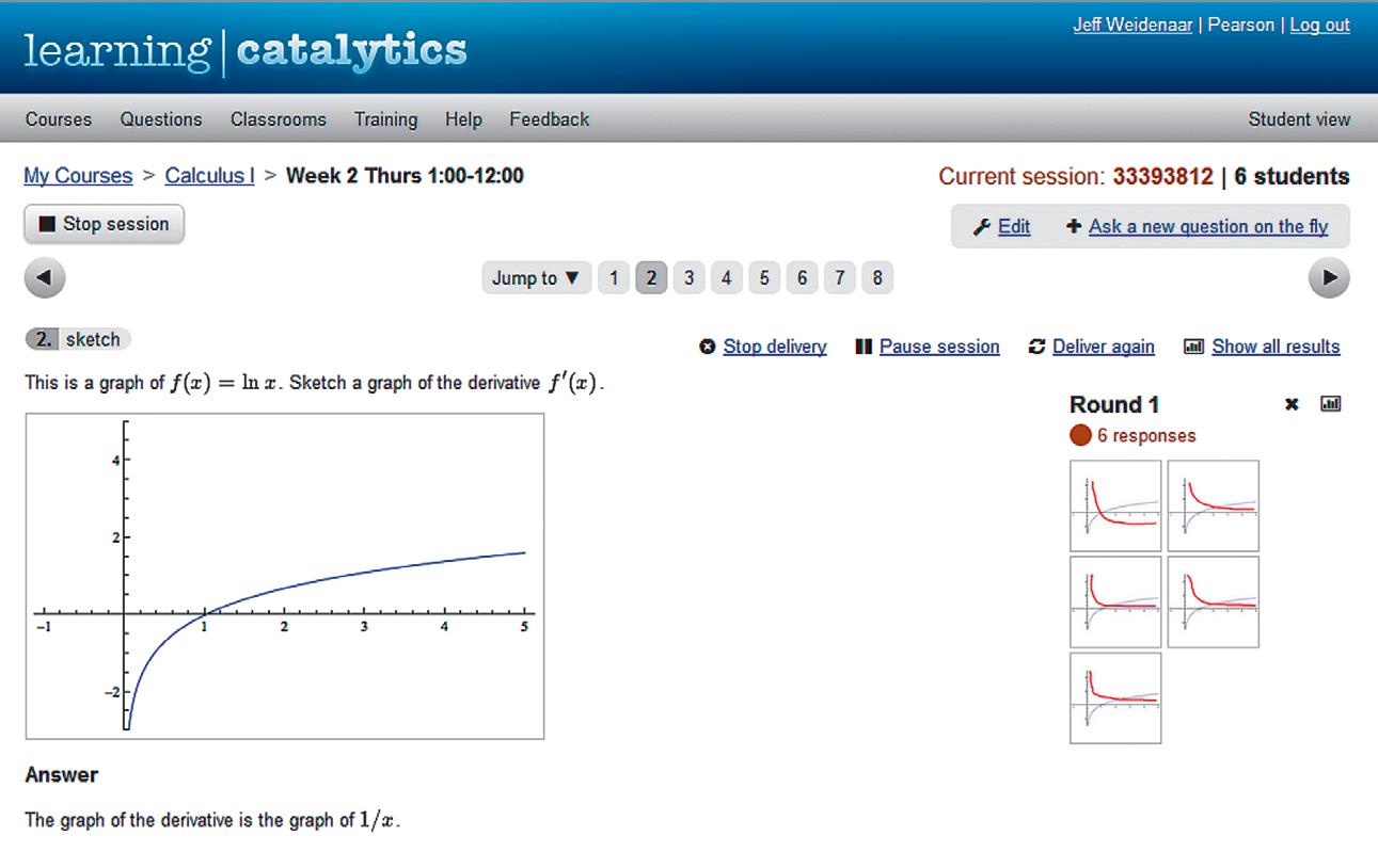
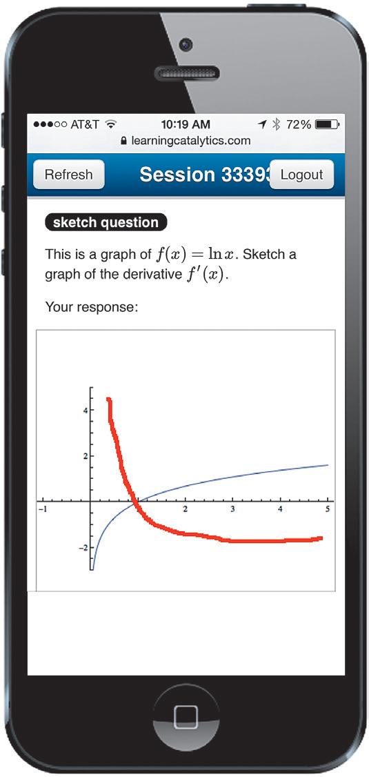
• Learning Catalytics™ is a student response tool that uses students’ smartphones, tablets, or laptops to engage them in more interactive tasks and thinking during lecture. Learning Catalytics fosters student engagement and peer-to-peer learning with realtime analytics. Learning Catalytics is available to all MyLab Math users.
Learning and Teaching Tools
• Interactive Figures illustrate key concepts and allow manipulation for use as teaching and learning tools. We also include videos that use the Interactive Figures to explain key concepts.
• Instructional videos—hundreds of videos are available as learning aids within exercises and for self-study. The Guide to Video-Based Assignments makes it easy to assign videos for homework by showing which MyLab Math exercises correspond to each video.
• The complete eText is available to students through their MyLab Math courses.
• PowerPoint Presentations that cover each section of the book are available for download.
• Mathematica manual and projects, Maple manual and projects, TI Graphing Calculator manual—These manuals cover Maple 17, Mathematica 8, and the TI-84 Plus and TI-89, respectively. Each provides detailed guidance for integrating the software package or graphing calculator throughout the course, including syntax and commands.
• Accessibility and achievement go hand in hand. MyLab Math is compatible with the JAWS screen reader, and it enables students to read and interact with multiple-choice and free-response problem types via keyboard controls and math notation input. MyLab Math also works with screen enlargers, including ZoomText, MAGic, and SuperNova. And, all MyLab Math videos have closed-captioning. More information is available at http://mymathlab.com/accessibility.
• A comprehensive gradebook with enhanced reporting functionality allows you to efficiently manage your course.
• The Reporting Dashboard offers insight as you view, analyze, and report learning outcomes. Student performance data is presented at the class, section, and program levels in an accessible, visual manner so you’ll have the information you need to
• Item Analysis tracks class-wide understanding of particular exercises so you can refine your class lectures or adjust the course/department syllabus. Just-in-time teaching has never been easier!
MyLab Math comes from an experienced partner with educational expertise and an eye on the future. Whether you are just getting started with MyLab Math, or have a question along the way, we’re here to help you learn about our technologies and how to incorporate them into your course. To learn more about how MyLab Math helps students succeed, visit www.mymathlab.com or contact your Pearson rep.
Instructor’s Solutions Manual (downloadable)
ISBN: 1-29-225326-6 | 978-1-29225326-8
The Instructor’s Solutions Manual contains complete worked-out solutions to all the exercises in Thomas’ Calculus. It can be downloaded from within MyLab Math or the Pearson Instructor Resource Center, www.pearsonglobaleditions.com/irc.
Student’s Solutions Manual
ISBN: 1-29-225331-2 | 978-1-29-225331-2
The Student’s Solutions Manual contains worked-out solutions to all the odd-numbered exercises in Thomas’ Calculus. These manuals can be downloaded from within MyLab Math.
Companion Website
The companion Website, located at www.pearsonglobaleditions.com, includes opportunities for practice and review.
Just-In-Time Algebra and Trigonometry for Calculus, Fourth Edition
ISBN: 0-321-67104-X | 978-0-321-67104-2
Sharp algebra and trigonometry skills are critical to mastering calculus, and Just-in-Time Algebra and Trigonometry for Calculus by Guntram Mueller and Ronald I. Brent is designed to bolster these skills while students study calculus. As students make their way through calculus, this brief supplementary text is with them every step of the way, showing them the necessary algebra or trigonometry topics and pointing out potential problem spots. The easy-to-use table of contents has topics arranged in the order in which students will need them as they study calculus. This supplement is available in printed form only (note that MyLab Math contains a separate diagnostic and remediation system for gaps in algebra and trigonometry skills).
Technology Manuals and Projects (downloadable)
Maple Manual and Projects by Marie Vanisko, Carroll College Mathematica Manual and Projects by Marie Vanisko, Carroll College TI-Graphing Calculator Manual by Elaine McDonald-Newman, Sonoma State University
These manuals and projects cover Maple 17, Mathematica 9, and the TI-84 Plus and TI89. Each manual provides detailed guidance for integrating a specific software package or graphing calculator throughout the course, including syntax and commands. The projects include instructions and ready-made application files for Maple and Mathematica. These materials are available to download within MyLab Math.
TestGen®
ISBN: 1-29-225332-0 | 978-1-29-225332-9
TestGen® (www.pearsoned.com/testgen) enables instructors to build, edit, print, and administer tests using a computerized bank of questions developed to cover all the objectives of the text. TestGen is algorithmically based, allowing instructors to create multiple but equivalent versions of the same question or test with the click of a button. Instructors can also modify test bank questions or add new questions. The software and test bank are available for download from Pearson Education’s online catalog, www.pearsonglobaleditions.com.
PowerPoint® Lecture Slides
ISBN: 1-29-225330-4 | 978-1-29-225330-5
These classroom presentation slides were created for the Thomas’ Calculus series. Key graphics from the book are included to help bring the concepts alive in the classroom. These files are available to qualified instructors through the Pearson Instructor Resource Center, www.pearsonglobaleditions.com/irc, and within MyLab Math.
Acknowledgments
We are grateful to Duane Kouba, who created many of the new exercises. We would also like to express our thanks to the people who made many valuable contributions to this edition as it developed through its various stages:
Accuracy Checkers
Thomas Wegleitner
Jennifer Blue
Lisa Collette
Reviewers for the Fourteenth Edition
Alessandro Arsie, University of Toledo
Doug Baldwin, SUNY Geneseo
Steven Heilman, UCLA
David Horntrop, New Jersey Institute of Technology
Eric B. Kahn, Bloomsburg University
Colleen Kirk, California Polytechnic State University
Mark McConnell, Princeton University
Niels Martin Møller, Princeton University
James G. O’Brien, Wentworth Institute of Technology
Alan Saleski, Loyola University Chicago
Alan Von Hermann, Santa Clara University
Don Gayan Wilathgamuwa, Montana State University
James Wilson, Iowa State University
The following faculty members provided direction on the development of the MyLab Math course for this edition.
Charles Obare, Texas State Technical College, Harlingen
Elmira Yakutova-Lorentz, Eastern Florida State College
C. Sohn, SUNY Geneseo
Ksenia Owens, Napa Valley College
Ruth Mortha, Malcolm X College
George Reuter, SUNY Geneseo
Daniel E. Osborne, Florida A&M University
Luis Rodriguez, Miami Dade College
Abbas Meigooni, Lincoln Land Community College
Nader Yassin, Del Mar College
Arthur J. Rosenthal, Salem State University
Valerie Bouagnon, DePaul University
Brooke P. Quinlan, Hillsborough Community College
Shuvra Gupta, Iowa State University
Alexander Casti, Farleigh Dickinson University
Sharda K. Gudehithlu, Wilbur Wright College
Deanna Robinson, McLennan Community College
Global Edition
Kai Chuang, Central Arizona College
Vandana Srivastava, Pitt Community College
Brian Albright, Concordia University
Brian Hayes, Triton College
Gabriel Cuarenta, Merced College
John Beyers, University of Maryland University College
Daniel Pellegrini, Triton College
Debra Johnsen, Orangeburg Calhoun Technical College
Olga Tsukernik, Rochester Institute of Technology
Jorge Sarmiento, County College of Morris
Val Mohanakumar, Hillsborough Community College
MK Panahi, El Centro College
Sabrina Ripp, Tulsa Community College
Mona Panchal, East Los Angeles College
Gail Illich, McLennan Community College
Mark Farag, Farleigh Dickinson University
Selena Mohan, Cumberland County College
The publishers would like to thank the following for their contribution to the Global Edition:
Contributor for the Fourteenth Edition in SI Units
José Luis Zuleta Estrugo received his PhD degree in Mathematical Physics from the University of Geneva, Switzerland. He is currently a faculty member in the Department of Mathematics in École Polytechnique Fédérale de Lausanne (EPFL), Switzerland, where he teaches undergraduate courses in linear algebra, calculus, and real analysis.
Reviewers for the Fourteenth Edition in SI Units
Fedor Duzhin, Nanyang Technological University
B. R. Shankar, National Institute of Technology Karnataka
Contributor for the Thirteenth Edition in SI Units
Antonio Behn, Universidad de Chile
Dedication
We regret that prior to the writing of this edition our coauthor Maurice Weir passed away. Maury was dedicated to achieving the highest possible standards in the presentation of mathematics. He insisted on clarity, rigor, and readability. Maury was a role model to his students, his colleagues, and his coauthors. He was very proud of his daughters, Maia Coyle and Renee Waina, and of his grandsons, Matthew Ryan and Andrew Dean Waina. He will be greatly missed.
Functions 1
OVERVIEW Functions are fundamental to the study of calculus. In this chapter we review what functions are and how they are visualized as graphs, how they are combined and transformed, and ways they can be classified.
1.1 Functions and Their Graphs
Functions are a tool for describing the real world in mathematical terms. A function can be represented by an equation, a graph, a numerical table, or a verbal description; we will use all four representations throughout this book. This section reviews these ideas.
Functions; Domain and Range
The temperature at which water boils depends on the elevation above sea level. The interest paid on a cash investment depends on the length of time the investment is held. The area of a circle depends on the radius of the circle. The distance an object travels depends on the elapsed time.
In each case, the value of one variable quantity, say y, depends on the value of another variable quantity, which we often call x. We say that “y is a function of x” and write this symbolically as y = ƒ(x) (“ y equals ƒ of x”).
The symbol ƒ represents the function, the letter x is the independent variable representing the input value to ƒ, and y is the dependent variable or output value of ƒ at x.
DEFINITION A function ƒ from a set D to a set Y is a rule that assigns a unique value ƒ(x) in Y to each x in D
The set D of all possible input values is called the domain of the function. The set of all output values of ƒ(x) as x varies throughout D is called the range of the function. The range might not include every element in the set Y. The domain and range of a function can be any sets of objects, but often in calculus they are sets of real numbers interpreted as points of a coordinate line. (In Chapters 13–16, we will encounter functions for which the elements of the sets are points in the plane, or in space.)
Often a function is given by a formula that describes how to calculate the output value from the input variable. For instance, the equation A = pr 2 is a rule that calculates the area A of a circle from its radius r. When we define a function y = ƒ(x) with a formula and the domain is not stated explicitly or restricted by context, the domain is assumed to
xf (x) f
Input (domain) Output (range)
FIGURE 1.1 A diagram showing a function as a kind of machine.
x a f (a) f (x)
D = domainset Y = setcontaining therange
FIGURE 1.2 A function from a set D to a set Y assigns a unique element of Y to each element in D.
be the largest set of real x-values for which the formula gives real y-values. This is called the natural domain of ƒ. If we want to restrict the domain in some way, we must say so. The domain of y = x 2 is the entire set of real numbers. To restrict the domain of the function to, say, positive values of x, we would write “ y = x 2 , x 7 0.”
Changing the domain to which we apply a formula usually changes the range as well. The range of y = x 2 is [0, q). The range of y = x 2 , x Ú 2, is the set of all numbers obtained by squaring numbers greater than or equal to 2. In set notation (see Appendix 1), the range is 5 x 2 x Ú 2 6 or 5 y y Ú 4 6 or 3 4, q).
When the range of a function is a set of real numbers, the function is said to be realvalued. The domains and ranges of most real-valued functions we consider are intervals or combinations of intervals. Sometimes the range of a function is not easy to find.
A function ƒ is like a machine that produces an output value ƒ(x) in its range whenever we feed it an input value x from its domain (Figure 1.1). The function keys on a calculator give an example of a function as a machine. For instance, the 2x key on a calculator gives an output value (the square root) whenever you enter a nonnegative number x and press the 2x key.
A function can also be pictured as an arrow diagram (Figure 1.2). Each arrow associates to an element of the domain D a single element in the set Y. In Figure 1.2, the arrows indicate that ƒ(a) is associated with a, ƒ(x) is associated with x, and so on. Notice that a function can have the same output value for two different input elements in the domain (as occurs with ƒ(a) in Figure 1.2), but each input element x is assigned a single output value ƒ(x).
EXAMPLE 1 Verify the natural domains and associated ranges of some simple functions. The domains in each case are the values of x for which the formula makes sense.
Function Domain (x) Range (y)
y = x 2 (- q, q) 3 0, q)
y = 1 > x (- q, 0) ∪ (0, q) (- q, 0) ∪ (0, q)
y = 2x 3 0, q) 3 0, q)
y = 24 - x (- q, 4 4 3 0, q)
y = 21 - x 2 3 - 1, 1 4 3 0, 1 4
Solution The formula y = x 2 gives a real y-value for any real number x, so the domain is (- q, q). The range of y = x 2 is 3 0, q) because the square of any real number is nonnegative and every nonnegative number y is the square of its own square root: y = 1 2y 22 for y Ú 0
The formula y = 1 > x gives a real y-value for every x except x = 0. For consistency in the rules of arithmetic, we cannot divide any number by zero. The range of y = 1 > x, the set of reciprocals of all nonzero real numbers, is the set of all nonzero real numbers, since y = 1 > (1 > y). That is, for y ≠ 0 the number x = 1 > y is the input that is assigned to the output value y.
The formula y = 2x gives a real y-value only if x Ú 0 The range of y = 2x is 3 0, q) because every nonnegative number is some number’s square root (namely, it is the square root of its own square).
In y = 24 - x , the quantity 4 - x cannot be negative. That is, 4 - x Ú 0, or x … 4. The formula gives nonnegative real y-values for all x … 4. The range of 24 - x is 3 0, q), the set of all nonnegative numbers.
The formula y = 21 - x 2 gives a real y-value for every x in the closed interval from - 1 to 1. Outside this domain, 1 - x 2 is negative and its square root is not a real number. The values of 1 - x 2 vary from 0 to 1 on the given domain, and the square roots of these values do the same. The range of 21 - x 2 is 3 0, 1 4
FIGURE 1.5 Graph of the function in Example 2.
Graphs of Functions
If ƒ is a function with domain D, its graph consists of the points in the Cartesian plane whose coordinates are the input-output pairs for ƒ. In set notation, the graph is
5 (x, ƒ(x)) x ∊ D 6 .
The graph of the function ƒ(x) = x + 2 is the set of points with coordinates (x, y) for which y = x + 2 Its graph is the straight line sketched in Figure 1.3.
The graph of a function ƒ is a useful picture of its behavior. If (x, y) is a point on the graph, then y = ƒ(x) is the height of the graph above (or below) the point x. The height may be positive or negative, depending on the sign of ƒ(x) (Figure 1.4).
FIGURE 1.3 The graph of ƒ(x) = x + 2 is the set of points (x, y) for which y has the value x + 2
FIGURE 1.4 If (x, y) lies on the graph of ƒ, then the value y = ƒ(x) is the height of the graph above the point x (or below x if ƒ(x) is negative).
EXAMPLE 2 Graph the function y = x 2 over the interval 3 - 2, 2 4
Solution Make a table of xy-pairs that satisfy the equation y = x 2 . Plot the points (x, y) whose coordinates appear in the table, and draw a smooth curve (labeled with its equation) through the plotted points (see Figure 1.5).
How do we know that the graph of y = x 2 doesn’t look like one of these curves?
To find out, we could plot more points. But how would we then connect them? The basic question still remains: How do we know for sure what the graph looks like between the points we plot? Calculus answers this question, as we will see in Chapter 4. Meanwhile, we will have to settle for plotting points and connecting them as best we can.
Representing a Function Numerically
We have seen how a function may be represented algebraically by a formula and visually by a graph (Example 2). Another way to represent a function is numerically, through a table of values. Numerical representations are often used by engineers and experimental scientists. From an appropriate table of values, a graph of the function can be obtained using the method illustrated in Example 2, possibly with the aid of a computer. The graph consisting of only the points in the table is called a scatterplot
EXAMPLE 3
Musical notes are pressure waves in the air. The data associated with Figure 1.6 give recorded pressure displacement versus time in seconds of a musical note produced by a tuning fork. The table provides a representation of the pressure function (in micropascals) over time. If we first make a scatterplot and then connect the data points (t, p) from the table, we obtain the graph shown in the figure.
(s) p (pressure mPa)
FIGURE 1.6 A smooth curve through the plotted points gives a graph of the pressure function represented by the accompanying tabled data (Example 3).
0.00271 - 0.141 0.00543 - 0.320
0.00289 - 0 309 0.00562 - 0 354
0.00307 - 0.348 0.00579 - 0.248
0.00325 - 0 248 0.00598 - 0 035
0.00344 - 0.041
The Vertical Line Test for a Function
Not every curve in the coordinate plane can be the graph of a function. A function ƒ can have only one value ƒ(x) for each x in its domain, so no vertical line can intersect the graph of a function more than once. If a is in the domain of the function ƒ, then the vertical line x = a will intersect the graph of ƒ at the single point (a, ƒ(a)) .
A circle cannot be the graph of a function, since some vertical lines intersect the circle twice. The circle graphed in Figure 1.7a, however, contains the graphs of two functions of x, namely the upper semicircle defined by the function ƒ(x) = 21 - x 2 and the lower semicircle defined by the function g (x) = - 21 - x 2 (Figures 1.7b and 1.7c).
Piecewise-Defined Functions
Sometimes a function is described in pieces by using different formulas on different parts of its domain. One example is the absolute value function
First formula
Second formula
FIGURE 1.8 The absolute value function has domain (- q, q) and range 3 0, q).
FIGURE 1.7 (a) The circle is not the graph of a function; it fails the vertical line test. (b) The upper semicircle is the graph of the function ƒ(x) = 21 - x 2 (c) The lower semicircle is the graph of the function g (x) = - 21 - x 2
whose graph is given in Figure 1.8. The right-hand side of the equation means that the function equals x if x Ú 0 , and equals - x if x 6 0 Piecewise-defined functions often arise when real-world data are modeled. Here are some other examples.
EXAMPLE 4 The function
FIGURE 1.9 To graph the function y = ƒ(x) shown here, we apply different formulas to different parts of its domain (Example 4).
FIGURE 1.10 The graph of the greatest integer function y = : x ; lies on or below the line y = x, so it provides an integer floor for x (Example 5).
First formula
Second formula
Third formula is defined on the entire real line but has values given by different formulas, depending on the position of x. The values of ƒ are given by y = - x when x 6 0, y = x 2 when 0 … x … 1, and y = 1 when x 7 1. The function, however, is just one function whose domain is the entire set of real numbers (Figure 1.9).
EXAMPLE 5 The function whose value at any number x is the greatest integer less than or equal to x is called the greatest integer function or the integer floor function. It is denoted : x ; . Figure 1.10 shows the graph. Observe that : 2.4 ; = 2, : 1.9 ; = 1, : 0 ; = 0, : - 1.2 ; = - 2, : 2 ; = 2, : 0.2 ; = 0, : - 0.3 ; = - 1, : - 2 ; = - 2.
EXAMPLE 6 The function whose value at any number x is the smallest integer greater than or equal to x is called the least integer function or the integer ceiling function. It is denoted < x = . Figure 1.11 shows the graph. For positive values of x, this function might represent, for example, the cost of parking x hours in a parking lot that charges $1 for each hour or part of an hour.
Increasing and Decreasing Functions
If the graph of a function climbs or rises as you move from left to right, we say that the function is increasing. If the graph descends or falls as you move from left to right, the function is decreasing.
DEFINITIONS Let ƒ be a function defined on an interval I and let x1 and x2 be two distinct points in I
1. If ƒ(x2) 7 ƒ(x1) whenever x1 6 x2, then ƒ is said to be increasing on I 2. If ƒ(x2) 6 ƒ(x1) whenever x1 6 x2, then ƒ is said to be decreasing on I
FIGURE 1.11 The graph of the least integer function y = < x = lies on or above the line y = x, so it provides an integer ceiling for x (Example 6).
It is important to realize that the definitions of increasing and decreasing functions must be satisfied for every pair of points x1 and x2 in I with x1 6 x2. Because we use the inequality 6 to compare the function values, instead of … , it is sometimes said that ƒ is strictly increasing or decreasing on I. The interval I may be finite (also called bounded) or infinite (unbounded).
EXAMPLE 7 The function graphed in Figure 1.9 is decreasing on (- q, 0) and increasing on (0, 1) . The function is neither increasing nor decreasing on the interval (1, q) because the function is constant on that interval, and hence the strict inequalities in the definition of increasing or decreasing are not satisfied on (1, q)
Even Functions and Odd Functions: Symmetry
The graphs of even and odd functions have special symmetry properties.
DEFINITIONS A function y = ƒ(x) is an even function of x if ƒ(- x) = ƒ(x), odd function of x if ƒ(- x) = - ƒ(x), for every x in the function’s domain.
(x, y () - x, y)
0 x y y = x 2
(a)
0 x y y = x 3 (x, y)
(- x, - y)
(b)
FIGURE 1.12 (a) The graph of y = x 2 (an even function) is symmetric about the y-axis. (b) The graph of y = x 3 (an odd function) is symmetric about the origin.
The names even and odd come from powers of x. If y is an even power of x, as in y = x 2 or y = x 4 , it is an even function of x because (- x)2 = x 2 and (- x)4 = x 4 . If y is an odd power of x, as in y = x or y = x 3 , it is an odd function of x because (- x)1 = - x and (- x)3 = - x 3 .
The graph of an even function is symmetric about the y-axis. Since ƒ(- x) = ƒ(x), a point (x, y) lies on the graph if and only if the point (- x, y) lies on the graph (Figure 1.12a). A reflection across the y-axis leaves the graph unchanged.
The graph of an odd function is symmetric about the origin. Since ƒ(- x) = - ƒ(x), a point (x, y) lies on the graph if and only if the point (- x, - y) lies on the graph (Figure 1.12b). Equivalently, a graph is symmetric about the origin if a rotation of 180° about the origin leaves the graph unchanged. Notice that the definitions imply that both x and - x must be in the domain of ƒ.
EXAMPLE 8 Here are several functions illustrating the definitions.
ƒ(x) = x 2
ƒ(x) = x 2 + 1
Even function: (- x)2 = x 2 for all x; symmetry about y-axis. So ƒ(- 3) = 9 = ƒ(3) . Changing the sign of x does not change the value of an even function.
Even function: (- x)2 + 1 = x 2 + 1 for all x; symmetry about y-axis (Figure 1.13a).
ƒ(x) = x Odd function: (- x) = - x for all x; symmetry about the origin. So ƒ(- 3) = - 3 while ƒ(3) = 3 . Changing the sign of x changes the sign of an odd function.
ƒ(x) = x + 1 Not odd: ƒ(- x) = - x + 1, but - ƒ(x) = - x - 1 The two are not equal.
Not even: (- x) + 1 ≠ x + 1 for all x ≠ 0 (Figure 1.13b).
FIGURE 1.13 (a) When we add the constant term 1 to the function y = x 2 , the resulting function y = x 2 + 1 is still even and its graph is still symmetric about the y-axis. (b) When we add the constant term 1 to the function y = x, the resulting function y = x + 1 is no longer odd, since the symmetry about the origin is lost. The function y = x + 1 is also not even (Example 8).
Common Functions
A variety of important types of functions are frequently encountered in calculus.
Linear Functions A function of the form ƒ(x) = mx + b , where m and b are fixed constants, is called a linear function. Figure 1.14a shows an array of lines ƒ(x) = mx . Each of these has b = 0, so these lines pass through the origin. The function ƒ(x) = x where m = 1 and b = 0 is called the identity function. Constant functions result when the slope is m = 0 (Figure 1.14b).
FIGURE 1.14 (a) Lines through the origin with slope m. (b) A constant function with slope m = 0
DEFINITION Two variables y and x are proportional (to one another) if one is always a constant multiple of the other—that is, if y = kx for some nonzero constant k.
If the variable y is proportional to the reciprocal 1 > x, then sometimes it is said that y is inversely proportional to x (because 1 > x is the multiplicative inverse of x).
Power Functions A function ƒ(x) = x a , where a is a constant, is called a power function There are several important cases to consider.