1 Introduction to Fatigue of Plastics and Elastomers
There are two recently published books on the properties of engineering plastics in this series. The Effect of Temperature and Other Factors on Plastics, Plastics Design Library [1] discusses the general mechanical properties of plastics. The mechanical properties as a function of temperature, humidity, and other factors are presented in graphs or tables. That work includes hundreds of graphs of stress versus strain, modulus versus temperature, impact strength versus temperature, etc. Time was not a factor in that book. The Effect of Creep and Other Time Related Factors on Plastics, Plastics Design Library [2] discusses the long-term behavior of plastics when exposed to constant stresses or strains for long periods of time. This book adds another two layers of plastics performance criteria, fatigue and tribology.
This book provides graphical multipoint data and tabular data on fatigue and tribological properties of plastics and elastomers along with introductory background to help in understanding those data. This chapter deals with the types of stress and an introduction to fatigue. Tribology is discussed in chapter: Introduction to the Tribology of Plastics and Elastomers. The chemistry of plastics follows in chapter: Introduction to Plastics and Polymers. The remaining chapters contain the data.
The idea of fatigue is very simple. If an object is subjected to a stress or deformation, and it is repeated, the object becomes weaker. This weakening of plastic material is called fatigue and occurs when the material is subject to alternating stresses, over a long period of time.
1.1 Types of Stress
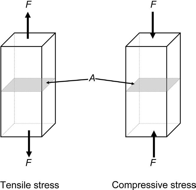
Fatigue occurs as a result of rapidly changing stress or strain. Stress and strain can be applied in a number of ways. Normal stress (σ ) is the ratio of the applied force (F) over the cross-sectional area (A) as shown in Eq. (1.1) and Fig. 1.1:
1.1.1 Tensile and Compressive Stress
When the applied force is directed away from the part, as shown in Fig. 1.1, it is a tensile force inducing a tensile stress. This is also called a normal stress as it is applied perpendicularly. When the force is applied toward the part, it is a compressive force inducing a compressive stress.
1.1.2 Shear Stress
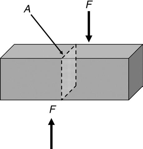
A shear stress (τ ) is defined as a stress which is applied parallel or tangential to a face of a material as shown in Fig. 1.2. The shear force is applied parallel to the cross-sectional area A
Figure 1.1 Illustration of tensile stress and compressive stress.
1.2
Figure
Illustration of shear stress.
Shear stress is also expressed as force per unit area as in Eq. (1.2):
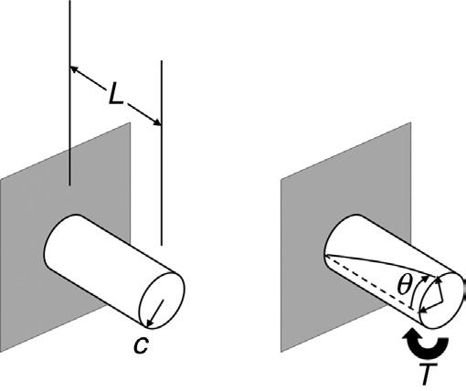
1.1.3 Torsional Stress
Torsional stress (τ ) occurs when a part such as a rod for shaft is twisted as in Fig. 1.3. This is also a shear stress, but the stress is variable and depends on how far the point of interest is from the center of the shaft. The equation describing torsional stress is shown in Eq. (1.3):
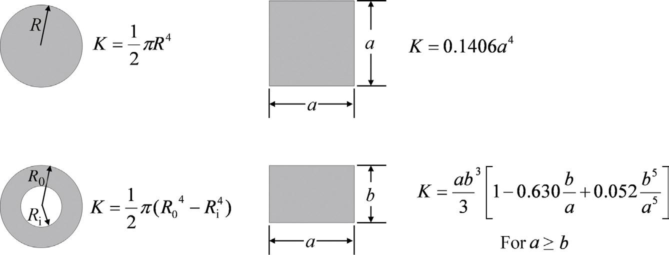
The torsional constant (K) is dependent on geometry and the formulas for several geometries are shown in Fig. 1.4. Additional formulas for torsional constant are published [3].
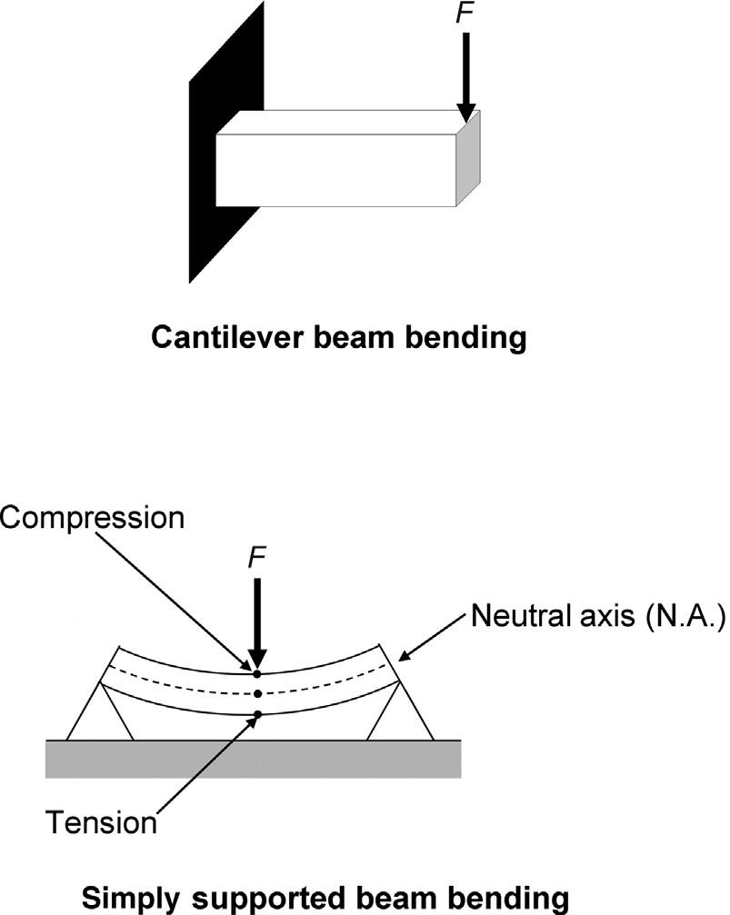
1.1.4 Flexural or Bending Stress
Bending stress or flexural stress commonly occurs in two instances, shown in Fig. 1.5. One is called a simply supported structural beam bending and the other is called cantilever bending. For the simply supported structural beam, the upper surface of the bending beam is in compression and the bottom surface is in tension. The neutral axis (NA) is a region of zero stress. The bending stress (σ ) is defined by Eq. (1.5). M is the bending moment, which
In Eq. (1.3), T is the torque and c is the distance from the center of the shaft or rod. K is a torsional constant that is dependent on the geometry of the shaft, rod, or beam. The torque (T) is further defined by Eq. (1.4), where u is the angle of twist, G is the modulus of rigidity (material dependent), and L is the length:
or bending stress.
1.4 Torsional constants for rods or beams of common geometries.
Figure 1.3 Illustration of torsional stress.
Figure
Figure 1.5 Illustration of flexural
is calculated by multiplying a force by the distance between that point of interest and the force. c is the distance from the NA (in Fig. 1.5) and I is the moment of inertia. The cantilevered beam configuration is also shown in Fig. 1.5 and has a similar formula. The formulas for M, c, and I can be complex, depending on the exact configuration and beam shape, but many are published [3].
σ = Mc I (1.5)
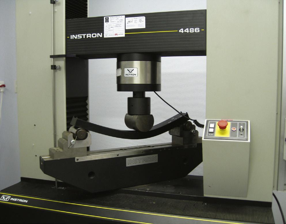
A picture of a supported beam-bending test in an Instron machine is shown in Fig. 1.6.
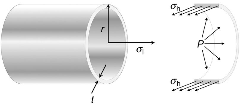
1.1.5 Hoop Stress
Hoop stress (σ h) is mechanical stress defined for rotationally symmetric objects such as pipe or tubing. The real-world view of hoop stress is the tension applied to the iron bands, or hoops, of a wooden barrel. It is the result of forces acting circumferentially. Fig. 1.7 shows stresses caused by pressure (P) inside a cylindrical vessel. The hoop stress is indicated on the right side of Fig. 1.7 that shows a segment of the pipe. The classic equation for hoop stress created by an internal pressure on a thin wall cylindrical pressure vessel is given in Eq. (1.6):
= Pr t h (1.6)
where P, the internal pressure; t, the wall thickness; r, the radius of the cylinder.
The SI unit for P is Pascal, while t and r are in meters.
If the pipe is closed on the ends, any force applied to them by internal pressure will induce an axial or longitudinal stress (σ l) on the same pipe wall. The longitudinal stress under the same conditions of Fig. 1.7 is given by Eq. (1.7):
There could also be a radial stress especially when the pipe walls are thick, but thin-walled sections often have negligibly small radial stress (σ r). The stress in radial direction at a point in the tube or cylinder wall is shown in Eq. (1.8):
where P, internal pressure in the tube or cylinder; a, internal radius of tube or cylinder; b, external radius of tube or cylinder; r, radius to point in tube where radial stress is calculated.
aThis is a file from the Wikimedia Commons which is a freely licensed media file repository.
Figure 1.6 Picture of a three-point flexural or bending test being done in an Instron universal testing machine.a
Figure 1.7 Illustration of hoop stress.
Often the stresses in pipe are combined into a measure called equivalent stress. This is determined using the Von Mises equivalent stress formula which is shown in Eq. (1.9):
where σ l, longitudinal stress; σ h, hoop stress; τc, tangential shear stress (from material flowing through the pipe).
Failure by fracture in cylindrical vessels is dominated by the hoop stress in the absence of other external loads because it is the largest principal stress. Failure by yielding is affected by an equivalent stress that includes hoop stress and longitudinal stress. The equivalent stress can also include tangential shear stress and radial stress when present.
1.2 Fatigue Testing
There are many machines that have been designed to put a periodic stress or strain on a test coupon or specimen. While the details of these machines vary, they really fall into similar designs. This section
will first present several basic fatigue test machine designs. Machines can be designed to put a cycling stress or a strain on the test coupon. The strain is a fixed displacement (% or mm/mm) and the stress is a pressure (MPa).
1.2.1 Fatigue Coupons
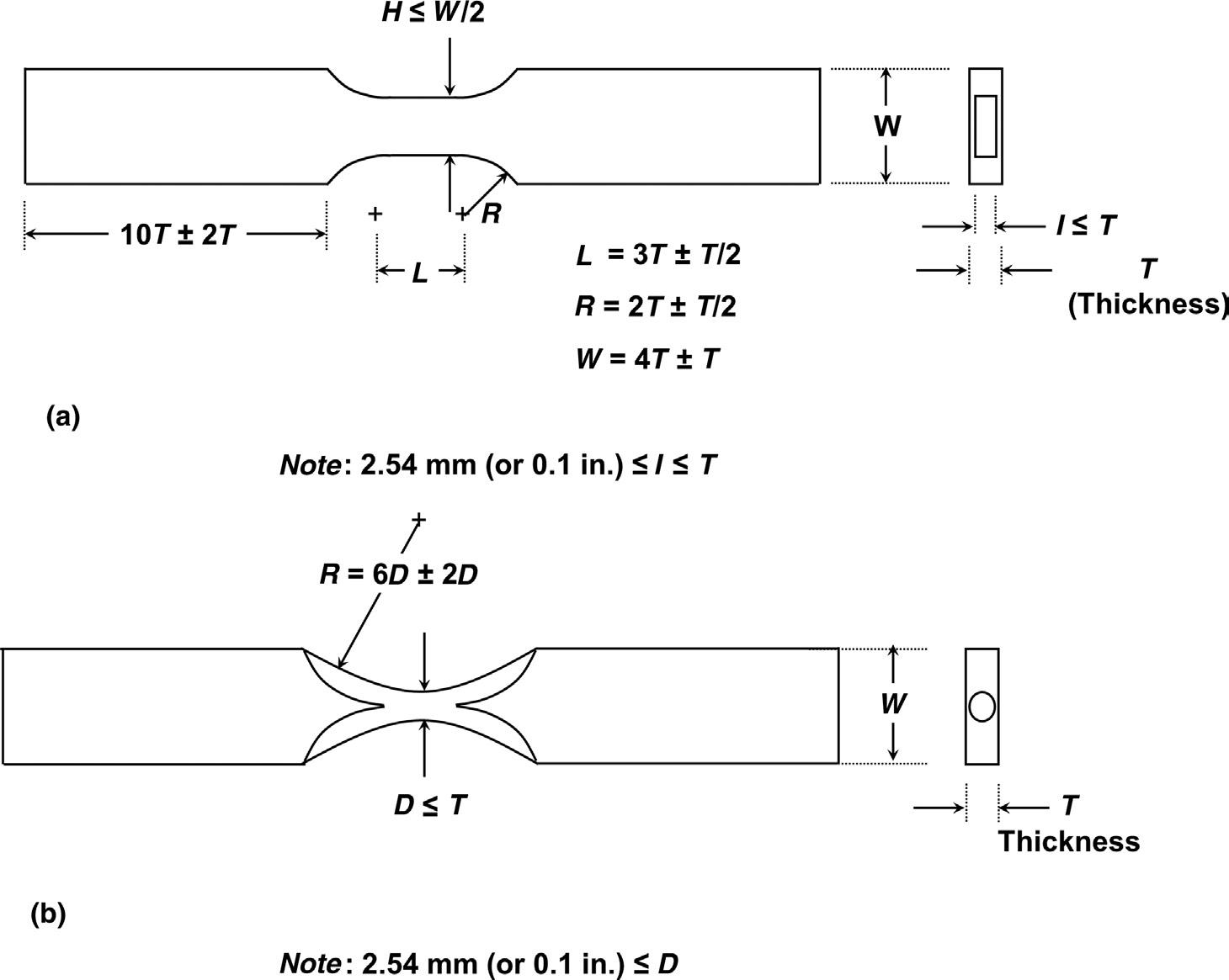
The test specimens are usually molded bars or rods that are further machined to specific shapes and configurations. ASTM International, originally known as the American Society for Testing and Materials (ASTM), is one organization that defines standard tests; its standards are the well-known ASTM standards. ASTM E606 describes fatigue specimens as shown in Figs. 1.8 and 1.9. Fig. 1.8 shows specimens that are made from molded sheet or bars. The test area is primarily in the center of these pieces. Specimen (a) in Fig. 1.8 has a rectangular cross-section while specimen (b) is circular.
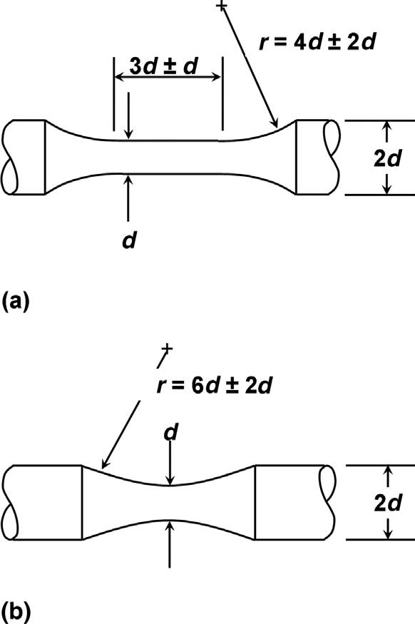
Specimens made from molded rods are shown in Fig. 1.9. The rods in this figure do not show the clamping options, of which there are many, to secure the specimen to the test machine.
Figure 1.8 Illustration of typical molded flat sheet fatigue-testing specimens. (a) Flat sheet fatigue specimen with rectangular cross-section; (b) flat sheet fatigue specimen with circular cross-section.
Figure 1.9 Illustration of typical molded rod fatiguetesting specimens. (a) Uniform-gage test section; (b) hourglass test section. Note : Dimension d (uniform to ±0.2%) is recommended to be 6.35 mm (0.25 in.). Dimension 2 d may be more or less depending on material hardness. End connections are not shown.
1.2.2 Tensile Eccentric Fatigue Machine
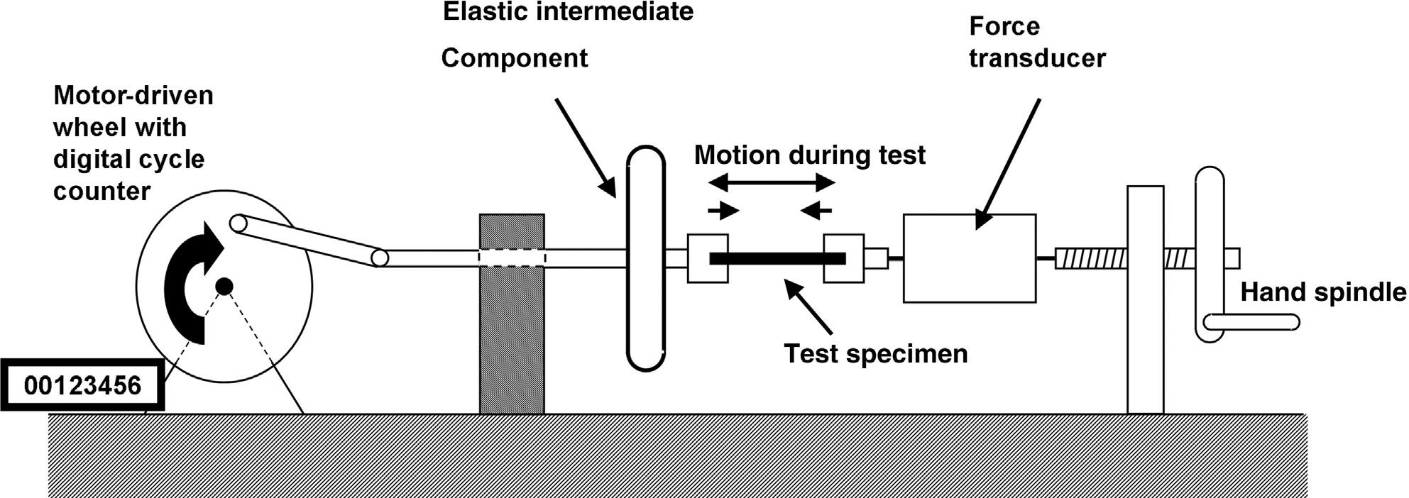
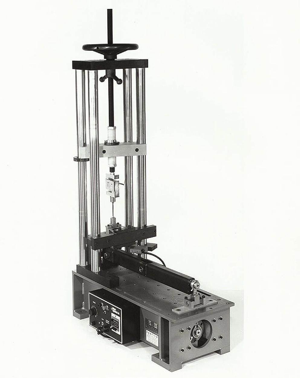
Many of the machines apply the stress or strain based on a circular drive mechanism and so they are called eccentric machines. One such machine for tensile and compressive testing is shown in Figs. 1.10 and 1.11. This machine may compress and extend a test specimen repeatedly.
A Sonntag testing machine is this type of device. In these tests, a stress is applied repeatedly at 1800 cycles/min to a test specimen until failure occurs. Specimens may be stressed in tension only, compression only, or both tension and compression, which is generally considered the most severe situation. In addition, fixtures can be used with this machine for producing flexure stresses.
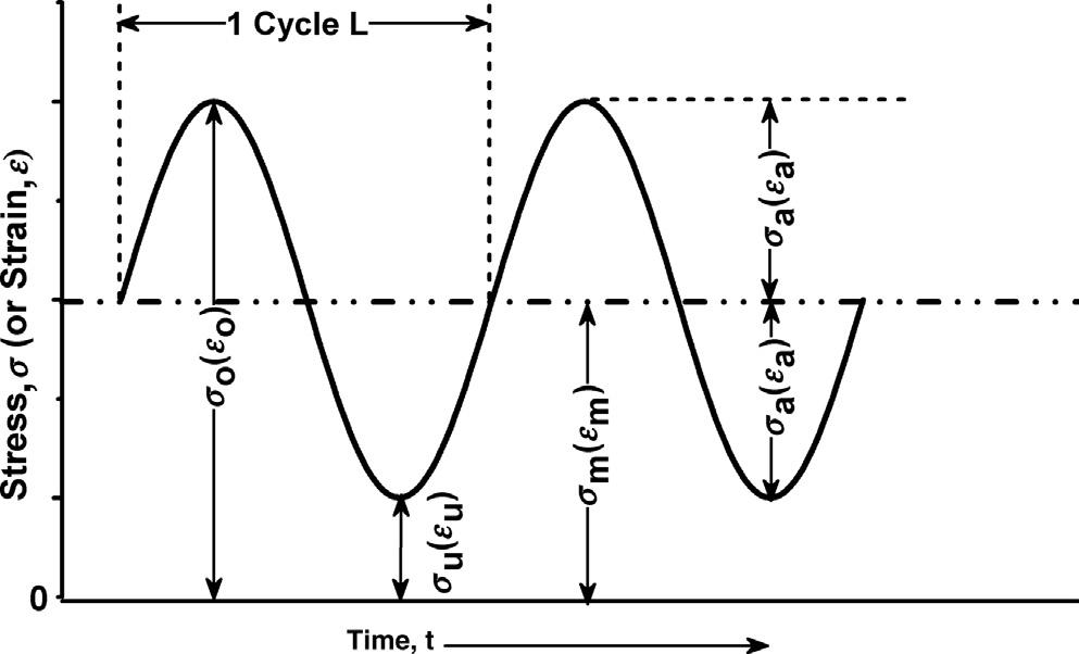
The stress and strain in eccentric machines vary in a sinusoidal manner as depicted in Fig. 1.12. This shows the change in stress or strain versus time. There are several descriptive parameters noted on this figure that are useful in specifying or describing the test conditions.
The terms and symbols are as follows:
L = cycle, one full oscillation of the loading (stress or strain), almost always assumed to be constant
f = cycle frequency; number of cycles per unit time in hertz
N = number of cycles
σ o = maximum stress, highest absolute stress value
σ u = minimum stress, lowest absolute stress value
σ m = mean stress = 0.5(σ o + σu)
σ a = stress amplitude = ±0.5(σ o σu)
ε o = maximum strain (displacement), highest absolute strain value
ε u = minimum strain (displacement), lowest absolute strain value
ε m = mean strain (displacement) = 0.5(ε o + εu)
ε a = strain (displacement) amplitude = ±0.5(ε o εu)
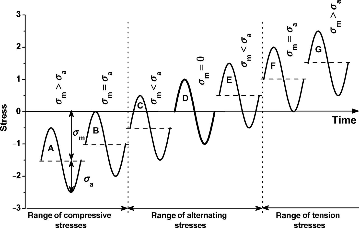
The mean stress, σm, or the mean strain, εm, is not always zero. A range of values is possible as shown
Figure 1.10 Diagram of an eccentric machine for tensile and compressive oscillation fatigue tests.
equal except that they differ by a negative sign. A real-world example of this type of stress cycle would be in an axle, in which every half-turn the stress on a point would be reversed. The most common type of cycle found in engineering applications is the other curves where the maximum stress and minimum stress are asymmetric, not equal and opposite. This type of stress cycle is called repeated stress cycle.
in Fig. 1.13. Curves A, D, and F are most common testing conditions. The simplest is the reversed stress cycle, Curve D. This is a sine wave where the maximum stress and minimum stress magnitudes are
The stroke set on the rotating wheel on the eccentric unit controls the strain/stress amplitude for the oscillation test. The mean stress is set using the hand spindle shown in Figs. 1.10 and 1.11. The cycle frequency is controlled by the rotational speed of the wheel. The frequency is often kept relatively low to minimize sample heating during the test. The mean and minimum stress can be set by adjusting the fixed
Figure 1.12 Illustration of the cyclic nature of the stress or strain with terms and symbols induced by eccentric test machines.
Figure 1.13 Illustration of the cyclic nature of the stress or strain and the ranges of mean stress offset (σm).
Figure 1.11 Photograph of an eccentric machine for tensile and compressive oscillation fatigue tests. Photo courtesy of Fatigue Dynamics, Inc.
clamping device. The stress amplitude may decrease during the test, which is caused by relaxation and heating. Correcting stress amplitude for this decrease requires increasing the eccentric stroke when the machine is turned off. To avoid any interruption to the test, an elastic intermediate component is incorporated in the test setup as shown in the figure, which considerably reduces the stress reduction, since its spring travel is greater than that of the plastic. This allows the machine to operate with quasiconstant stress values.
1.2.3 Flexural Eccentric Fatigue Machine
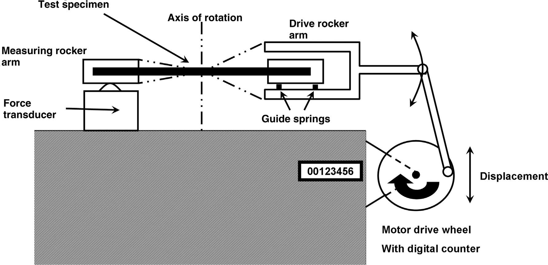
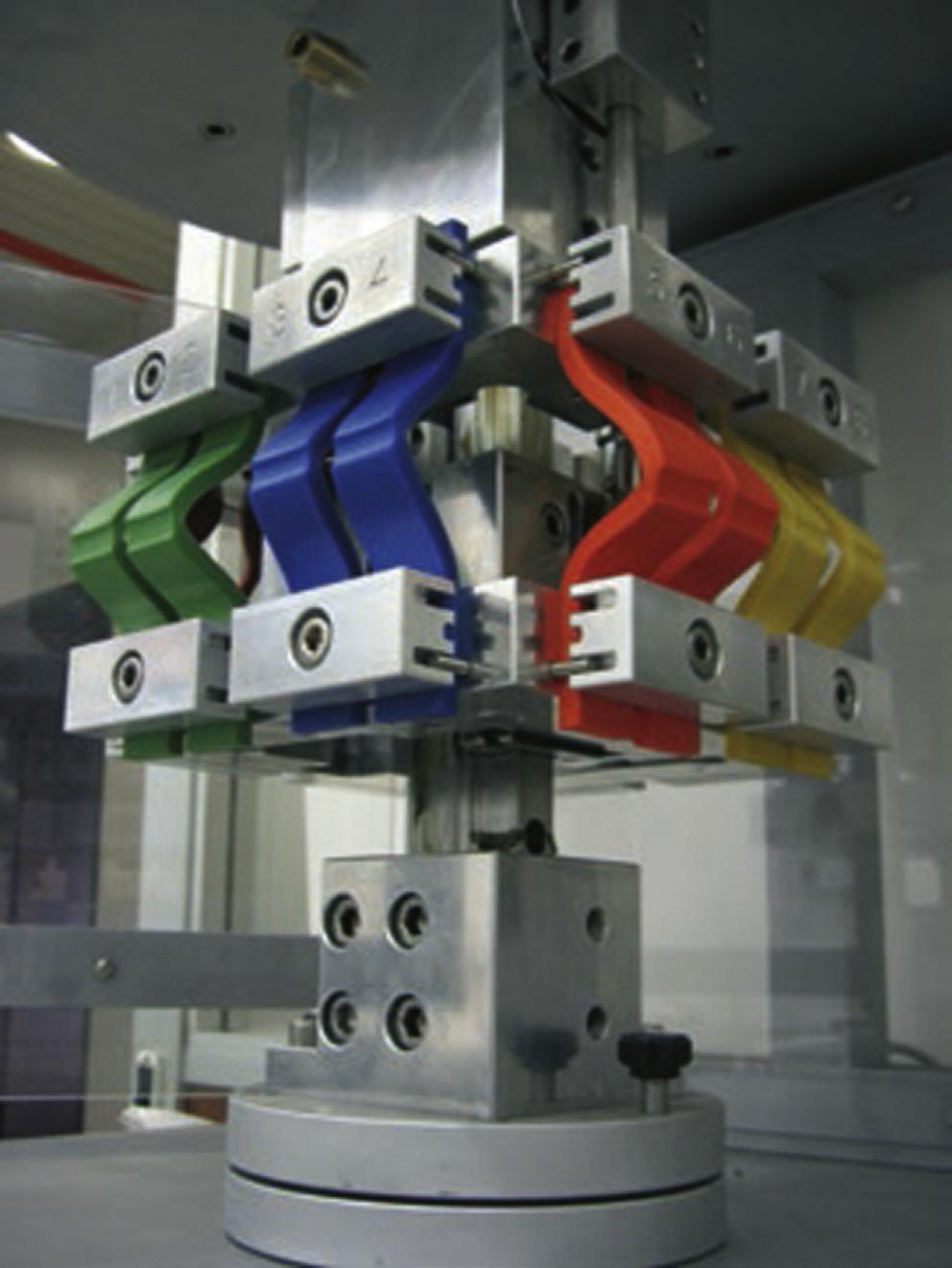
An eccentric machine for flexural fatigue testing is shown in Figs. 1.14 and 1.15. The stroke on this type of flexural unit imposes a constant bending radius on the specimen during the fatigue test at the axis of rotation in the figure. The guide springs under the right-hand clamping unit permit the specimen to move in the longitudinal direction which reduces the additional tensile forces that would otherwise develop during bending.
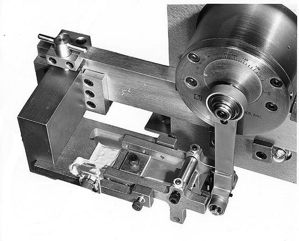
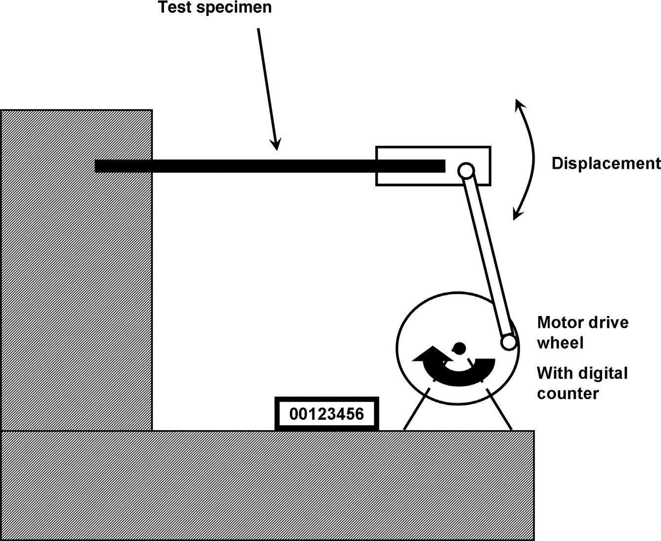
1.2.4 Cantilevered Beam Eccentric Flexural Fatigue Machine
The cantilevered beam flexural fatigue machine shown in Fig. 1.16 is similar to the machine shown
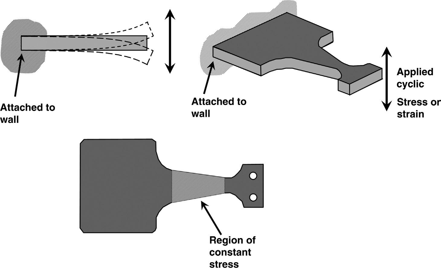
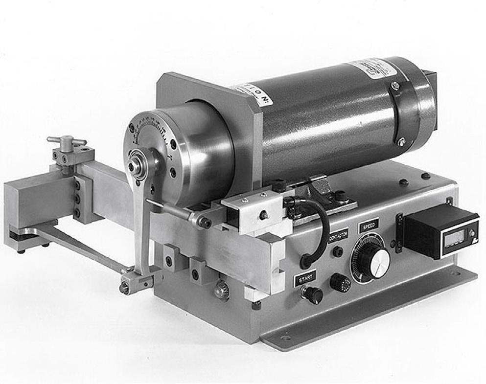
in Fig. 1.14 except that the test specimen is fixed and immovable at one end. ASTM D671 describes this test. Test specimen is supported as a cantilevered beam and is subjected to an alternating force at one end as shown in Fig. 1.17. The alternating applied stress and the cycles to failure are recorded. The “odd” triangular shape of the test specimen is designed to produce a constant stress along the length of the test section of the specimen. The machine that is used to perform this test is shown in Fig. 1.18
Figure 1.14 Illustration of an eccentric machine for flexural oscillation fatigue tests.
Figure 1.15 Photograph of an eccentric machine for flexural oscillation fatigue tests.
Photo courtesy of Fatigue Dynamics, Inc.
1.16 Diagram of a cantilevered fatigue-testing machine.
Figure 1.17 Illustration of cantilevered fatigue-testing specimens per ASTM D671.
1.2.5 Servohydraulic, Electrohydraulic, or Pulsator Fatigue Testing Machines
Servohydraulic, electrohydraulic, or pulsator fatigue-testing machines do not use an eccentric wheel to apply cyclic stress and strain. These machines use a computer-controlled hydraulic drive or
pulsator to apply the varying stress or strain to the test specimen. This is particularly important because some real-world cycle modes have stress level and frequency varies randomly. Waveforms do not need to be limited to sine waves either. A real-world example of this situation is the simulation of the function of automobile shocks, where the frequency and magnitude of imperfections in the road will produce
Figure
courtesy of Fatigue Dynamics, Inc.
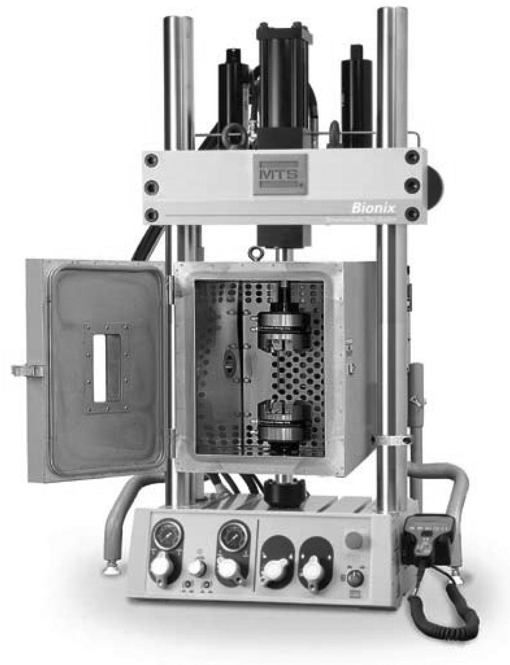
varying minimum and maximum stresses. Fig. 1.19 shows a picture of a servohydraulic machine. These machines may apply compressive, tensile, or flexural loads. The pulsator in Fig. 1.19 is located at the top.
The machines are usually run in a force- or stresscontrolled manner. This particular example includes an environmental chamber which can be used to control the temperature, humidity, and atmosphere the fatigue test will take place in.
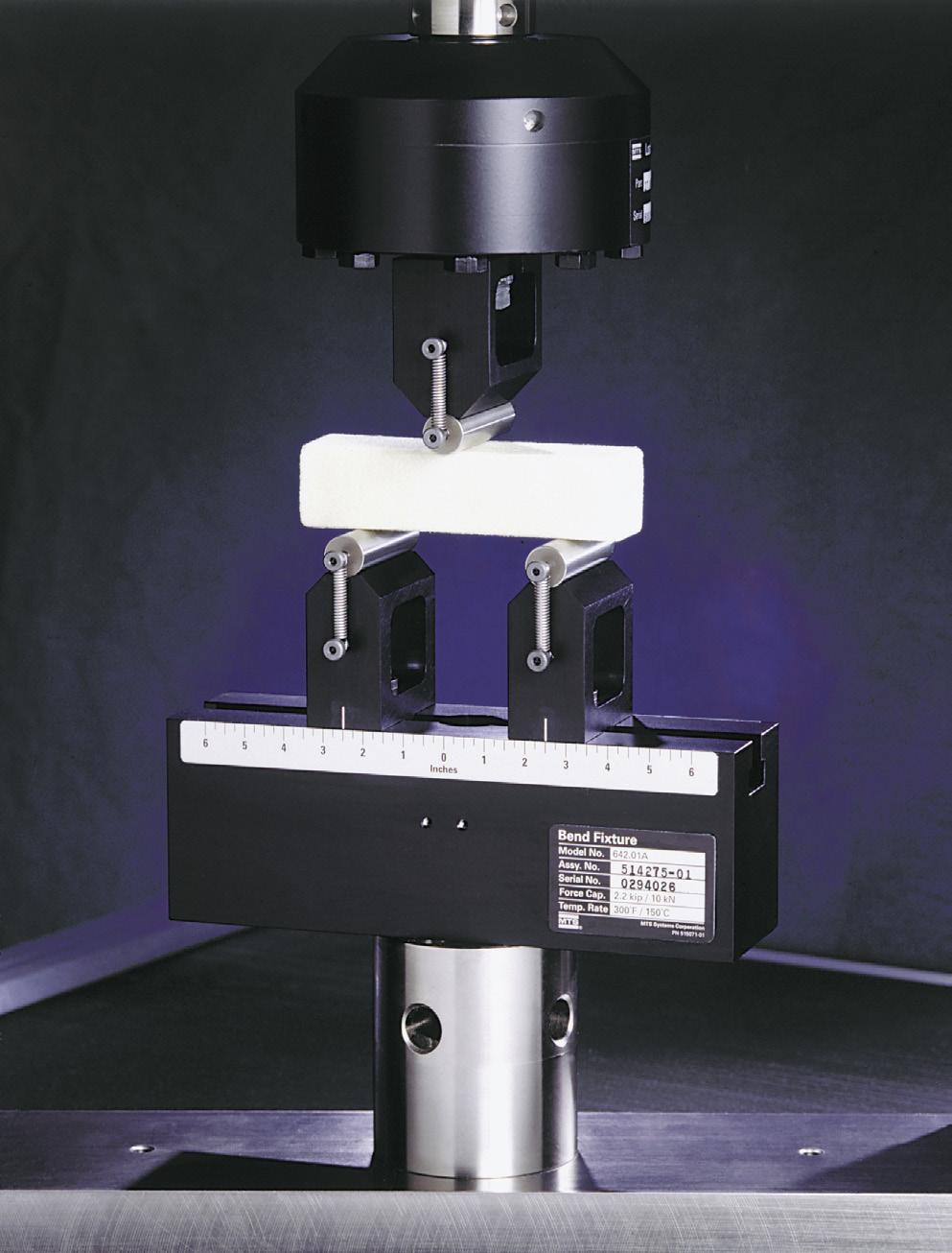
This machine can be run in a pulsating bending or flexing mode by utilizing a testing stage such as that shown in Fig. 1.20. The specimen is supported by roller bearings and is subjected to three-point bending. The bearings minimize the generated tensile stresses.
1.2.6 Ultrasonic Fatigue
The ultrasonic test machine is a fairly recent development [4,5]. These machines use a piezoelectric transducer to apply small rapid stresses at up to 20,000 cycles/s. At this rate 109 cycles can be applied in about 14 h and 1010 cycles take 6 days, which makes long-term testing more practical. Shimadzu Corporation produces the USF-2000 Ultrasonic Fatigue Test System.
Figure 1.18 Photograph of a cantilevered fatiguetesting machine.
Photo
Figure 1.19 Photograph of a servohydraulic fatiguetesting machine with environmental chamber.
Photo courtesy of MTS Systems Corporation © 2009.
Figure 1.20 Photograph of a flexural test rig used in a servohydraulic fatigue-testing machine.
Photo courtesy of MTS Systems Corporation © 2009.
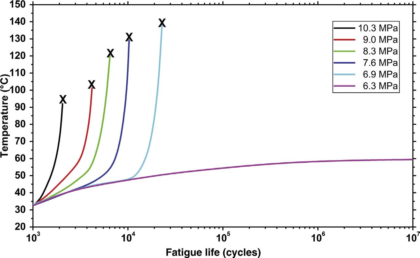
Figure 1.21 Measured temperature of PTFE samples undergoing fatigue testing at various constant stress levels at 30 Hz [6] X, failure.
1.2.7 Fatigue-Testing Method
Usually a minimum of six identical testing specimens are made for testing. A specimen is tested first at the highest stress or strain amplitude. It is tested until it fails (breaks). The stress/strain amplitude is recorded along with the cycles it took to fail. Because of the variability in the test, measurements are usually replicated a second or third time at the same stress/ strain amplitude. Next the stress/strain is reduced and the test is run till failure, which of course takes longer. The reduction in stress or strain continues until failure does not occur in 106–107 cycles.
A specimen may fail to break even at the highest stress or strain. In cases such as these, it is necessary to specify the number of cycles up to a particular level of material damage (eg, 20% stress reduction if strain is controlled, or 20% increase in strain if stress is controlled) instead of the number of cycles to failure.
The temperature of the specimen is monitored while testing as the specimen may heat up during the test. This process is referred to as hysteretic heating. Temperature is measured at the surface either by thermocouples that are attached to the surface or by noncontact infrared thermometers. Fig. 1.21 and Table 1.1 show examples of heating in polytetrafluoroethylene (PTFE) during fatigue testing.
The data shown in Fig. 1.21 and Table 1.1 do show the effect of temperature rise, and that it is most significant as the material being tested approaches failure.
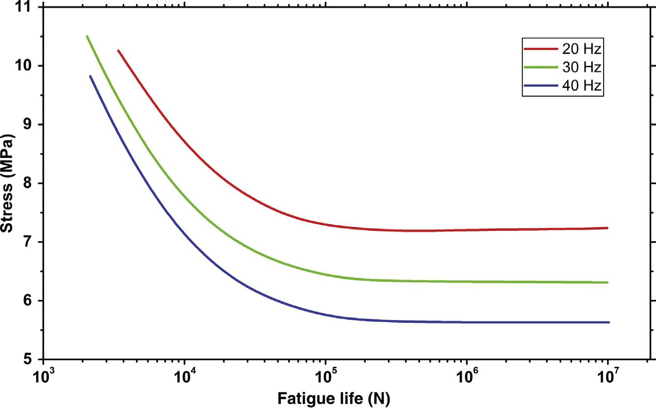
Frequency also affects fatigue testing because it also contributes to hysteretic temperature rise. An example of this is shown in Fig. 1.22. The significance of this curve is explained in a later section.
Most fatigue tests are conducted at room temperature with a cycle frequency, f, of 7 Hz, but the cycle frequency may be adjusted to minimize temperature rise and reduce testing time. Fatigue tests in all three loading ranges (compressive, alternating, and tension) can be conducted on the eccentric testing machines. These machines impart a constant strain. The measured imparted stress amplitude may become smaller with an increasing number of cycles if the specimen relaxes and heats up.
The plotting and analysis of the data is discussed in a later section of this chapter.
1.2.8 Flex Life Machines
There are several common flex life machines including MIT Flex, Ross Flex, and DeMattia Flex. The MIT Flex test is used to measure the ability of plastic films to withstand fatigue from flexing. This
Table 1.1 Measured Temperature at Failure of PTFE Samples Undergoing Fatigue Testing at Various Constant Stress Levels at 30 Hz [4]
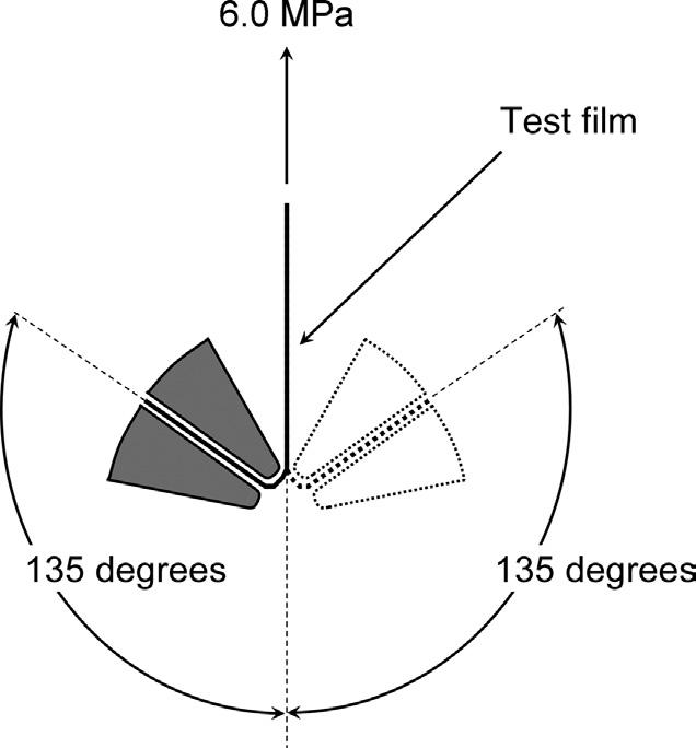
test method is described in ASTM D2176-97a(2007) Standard Test Method for Folding Endurance of Paper by the M.I.T. Tester (Withdrawn 2010), which is the standard method for testing the endurance of paper with the MIT test apparatus. A diagram of the flex held in the MIT Flex tester is shown in Fig. 1.23. One end of the plastic test film is clamped in a holder that rotates through 270 degrees very rapidly. The other end is pulled with a constant stress. Even though the ASTM standard describes a paper test, it can be applied to any thin film plastic. It is often used in the evaluation of wire plastic insulation. This test may also help provide insight into the effect of tensioning on life. Flex testing is occasionally performed after exposing the plastics to heat and/or chemicals in order to simulate use exposure conditions. The flex life is the number of cycles before the film breaks.
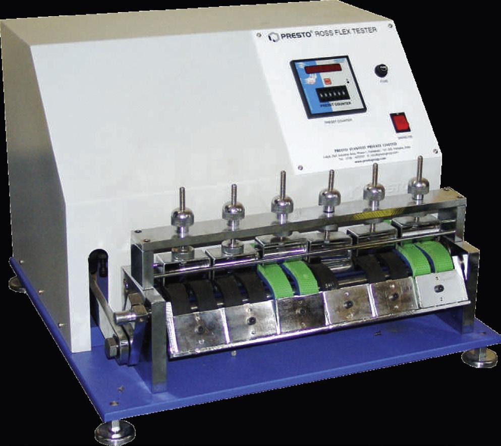
The Ross Flex test is defined in ASTM D105209(2014) Standard Test Method for Measuring Rubber Deterioration—Cut Growth Using Ross Flexing Apparatus. A pierced strip test specimen of 6.35 mm (0.25 in.) thickness is bent freely over a rod to a 90-degree angle and the cut length is measured at frequent intervals to determine the cut growth rate. The cut is initiated by a special shape-piercing tool. A multispecimen Ross Flex tester is shown in Fig. 1.24
The DeMattia Flex test is described in ASTM D813-07(2014) Standard Test Method for Rubber Deterioration—Crack Growth. A pierced strip test specimen of 6.35 mm (0.25 in.) thickness with a
Figure 1.22 The effect of testing frequency on the fatigue properties of polytetrafluoroethylene [7].
Figure 1.23 Illustration of mode of operation of the MIT Flex Life tester.
Figure 1.24 Photograph of a Ross Flex tester. Photo courtesy of Presto® Testing Instruments.
circular groove is restrained so that it becomes the outer surface of the bend specimen, with 180-degree bend, and the cut length is measured at frequent intervals to determine the cut growth rate. A multispecimen DeMattia Flex tester is shown in Fig. 1.25.
1.2.9 Fatigue and Fracture Standards
There are many testing or standards agencies that have standards concerning fatigue and fracture. Some of them include the following:
• ASTM—ASTM International, originally known as the American Society for Testing and Materials
• ISO—ISO (International Organization for Standardization)
• DIN—Deutsches Institut für Normung (German Institute for Standardization)
• ANSI—American National Standards Institute
• JIS—Japanese Industrial Standards
• SAE—Society of Automotive Engineers
Tables 1.2–1.5 list many, but not all, of the test standards. The individual organizations should be contacted for the details of these tests.
Table 1.2 ASTM Fatigue-Related Standards (ASTM International, West Conshohocken, PA, www.astm.org)
Standard Designation
E467-08(2014)
E194-98(2010)e1
E2208-02(2010)e1
E2443-05(2010)e1
E647-15
E1457-13
E1681-03(2013)
E466-15
E468-90(2004)e1
Standard Title
Standard Practice for Verification of Constant Amplitude Dynamic Forces in an Axial Fatigue Testing System
Standard Guide for Evaluating Data Acquisition Systems Used in Cyclic Fatigue and Fracture Mechanics Testing
Standard Guide for Evaluating Non-Contacting Optical Strain Measurement Systems
Standard Guide for Verifying Computer-Generated Test Results Through the Use Of Standard Data Sets
Standard Test Method for Measurement of Fatigue Crack Growth Rates
Standard Test Method for Measurement of Creep Crack Growth Times in Metals
Standard Test Method for Determining a Threshold Stress Intensity Factor for Environment-Assisted Cracking of Metallic Materials
Standard Practice for Conducting Force Controlled Constant Amplitude Axial Fatigue Tests of Metallic Materials
Standard Practice for Presentation of Constant Amplitude Fatigue Test Results for Metallic Materials
Figure 1.25 Photograph of a DeMattia Flex tester. Photo courtesy of Gibitre Instruments.
Table 1.2 ASTM Fatigue-Related Standards (ASTM International, West Conshohocken, PA, www.astm.org) (cont.)
Standard Designation
E606-12
E1922-04(2015)
E2207-15
E2244-15a
E2245-11
E2246-011
E2368-10
E2444-11
E399-12e3
E561-10e2
E740-03
E1221-12a
E1290-08e1
E1820-08a
E1921-15
E2472-12e1
E338-03(2014)
E436-03(2008)
E602-03
E1304-97(2014)
E1823-13
E739-10
E1049-85(2011)
D2176-97a(2007)
Standard Title
Standard Practice for Strain-Controlled Fatigue Testing
Standard Test Method for Translaminar Fracture Toughness of Laminated and Pultruded Polymer Matrix Composite Materials
Standard Practice for Strain-Controlled Axial-Torsional Fatigue Testing With Thin-Walled Tubular Specimens
Standard Test Method for In-Plane Length Measurements of Thin, Reflecting Films Using an Optical Interferometer
Standard Test Method for Residual Strain Measurements of Thin, Reflecting Films Using an Optical Interferometer
Standard Test Method for Strain Gradient Measurements of Thin, Reflecting Films Using an Optical Interferometer
Standard Practice for Strain Controlled Thermomechanical Fatigue Testing
Terminology Relating to Measurements Taken on Thin, Reflecting Films
Standard Test Method for Linear-Elastic Plane-Strain Fracture Toughness K Ic of Metallic Materials
Standard Test Method for K–R Curve Determination
Standard Practice for Fracture Testing with Surface-Crack Tension Specimens
Standard Test Method for Determining Plane-Strain Crack-Arrest Fracture Toughness, KIa, of Ferritic Steels
Standard Test Method for Crack-Tip Opening Displacement (CTOD) Fracture Toughness Measurement
Standard Test Method for Measurement of Fracture Toughness
Standard Test Method for Determination of Reference Temperature, To, for Ferritic Steels in the Transition Range
Standard Test Method for Determination of Resistance to Stable Crack Extension Under Low-Constraint Conditions
Standard Test Method of Sharp-Notch Tension Testing of High-Strength Sheet Materials
Standard Test Method for Drop-Weight Tear Tests of Ferritic Steels
Standard Test Method for Sharp-Notch Tension Testing With Cylindrical Specimens
Standard Test Method for Plane-Strain (Chevron-Notch) Fracture Toughness of Metallic Materials
Standard Terminology Relating to Fatigue and Fracture Testing
Standard Practice for Statistical Analysis of Linear or Linearized Stress–Life (S–N) and Strain–Life (ε–N) Fatigue Data
Standard Practices for Cycle Counting in Fatigue Analysis
Standard Test Method for Folding Endurance of Paper by the M.I.T. Tester
Table 1.3 ISO Fatigue-Related Standards (International Organization for Standardization, www.iso.org)
Standard Designation
ISO 1099:2006
ISO 1143:2010
ISO 12106:2003
ISO 12107:2012
ISO 12108:2012
ISO 13003:2003
ISO 1352:1977
ISO 24999:2008
ISO 27727:2008
ISO 3800:1993
ISO 4664-1:2011
ISO 4666-1:2010
ISO 4666-3:2010
ISO 4666-4:2007
ISO 4965:1979
ISO 5999:2007
ISO 1099:2006
ISO 1143:2010
ISO 12106:2003
ISO 12107:2012
ISO 12108:2012
ISO 13003:2003
ISO 1352:2011
ISO 24999:2008
ISO 27727:2008
ISO 3800:1993
Standard Title
Metallic materials—Fatigue testing—Axial force-controlled method
Metals—Rotating bar bending fatigue testing
Metallic materials—Fatigue testing—Axial-strain-controlled method
Metallic materials—Fatigue testing—Statistical planning and analysis of data
Metallic materials—Fatigue testing—Fatigue crack growth method
Fibre-reinforced plastics—Determination of fatigue properties under cyclic loading conditions
Steel—Torsional stress fatigue testing
Flexible cellular polymeric materials—Determination of fatigue by a constant-strain procedure
Rubber, vulcanized—Measurement of fatigue crack growth rate
Threaded fasteners—Axial load fatigue testing—Test methods and evaluation of results
Rubber, vulcanized or thermoplastic—Determination of dynamic properties—Part 1: General guidance
Rubber, vulcanized—Determination of temperature rise and resistance to fatigue in flexometer testing—Part 1: Basic principles
Rubber, vulcanized—Determination of temperature rise and resistance to fatigue in flexometer testing—Part 3: Compression flexometer
Rubber, vulcanized—Determination of temperature rise and resistance to fatigue in flexometer testing—Part 4: Constant-stress flexometer
Axial load fatigue testing machines—Dynamic force calibration—Strain gauge technique
Flexible cellular polymeric materials—Polyurethane foam for load-bearing applications excluding carpet underlay—Specification
Metallic materials—Fatigue testing—Axial force-controlled method
Metals—Rotating bar bending fatigue testing
Metallic materials—Fatigue testing—Axial-strain-controlled method
Metallic materials—Fatigue testing—Statistical planning and analysis of data
Metallic materials—Fatigue testing—Fatigue crack growth method
Fibre-reinforced plastics—Determination of fatigue properties under cyclic loading conditions
Steel—Torsional stress fatigue testing
Flexible cellular polymeric materials—Determination of fatigue by a constant-strain procedure
Rubber, vulcanized—Measurement of fatigue crack growth rate
Threaded fasteners—Axial load fatigue testing—Test methods and evaluation of results
Table 1.3 ISO Fatigue-Related Standards (International Organization for Standardization, www.iso.org) (cont.)
Standard Designation
ISO 4664-1:2011
ISO 4666-1:2010
ISO 4666-3:2010
ISO 4666-4:2007
ISO 4965:2012
ISO 5999:2007
ISO 6943:2007
ISO/AWI 12108
ISO/CD 1143
ISO/CD 12107
ISO/CD 1352
ISO/DIS 12111
Standard Title
Rubber, vulcanized or thermoplastic—Determination of dynamic properties—Part 1: General guidance
Rubber, vulcanized—Determination of temperature rise and resistance to fatigue in flexometer testing—Part 1: Basic principles
Rubber, vulcanized—Determination of temperature rise and resistance to fatigue in flexometer testing—Part 3: Compression flexometer
Rubber, vulcanized—Determination of temperature rise and resistance to fatigue in flexometer testing—Part 4: Constant-stress flexometer
Axial load fatigue testing machines—Dynamic force calibration -- Strain gauge technique
Flexible cellular polymeric materials—Polyurethane foam for load-bearing applications excluding carpet underlay—Specification
Rubber, vulcanized—Determination of tension fatigue
Metallic materials—Fatigue testing—Fatigue crack growth method
Metallic materials—Rotating bar bending fatigue testing
Metallic materials—Fatigue testing—Statistical planning and analysis of data
Metallic materials—Torsional stress fatigue testing
Metallic materials—Fatigue testing—Strain-controlled thermomechanical fatigue testing method
Table 1.4 DIN Fatigue-Related Standards (German Institute for Standardization, www.ihs.com)
Standard Designation
DIN 50113:1982
DIN 50142:1982
DIN EN ISO 5999
Standard Title
Testing of metals; Rotating bar bending fatigue test
Testing of metallic materials; Flat bending fatigue test
Polymeric materials, cellular flexible—Polyurethane foam for load-bearing applications excluding carpet underlay
Table 1.5 JIS Fatigue-Related Standards (Japanese Industrial Standards, https://www.jisc.go.jp/eng/)
Standard Designation
K 6265:20 01
K 7082:1993
K 7083:1993
K 7118:1995
K 7119:1972
Standard Title
Rubber, vulcanized and thermoplastic—Determination of temperature rise and resistance to fatigue in flexometer testing
Testing method for complete reversed plane bending fatigue of carbon fibre reinforced plastics
Testing method for constant-load amplitude tension–tension fatigue of carbon fibre reinforced plastics
General rules for testing fatigue of rigid plastics
Testing method of flexural fatigue of rigid plastics by plane bending
1.3 Understanding Fatigue-Testing Data
This section develops an understanding of what happens to a specimen during fatigue testing and describes various ways of reporting fatigue-testing results.
1.3.1 Monotonic Stress–Strain Behavior
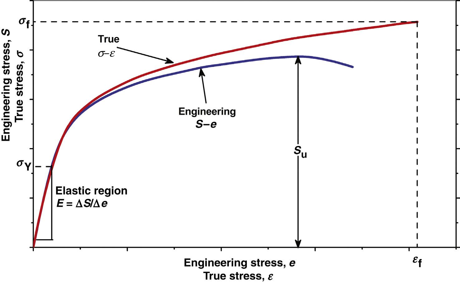
Monotonic stress–strain curves such as the one shown in Fig. 1.26 are very common. They are used to obtain design parameters for limiting stresses on structures and components subjected to static loading. They are frequently measured at a series of temperatures or strain rates as shown in an earlier book of this series [1]
The engineering stress–strain curve shown in Fig. 1.26 is obtained by means of a tension test, in which a specimen is subjected to a continually increasing, monotonic load. The elongation of the specimen is measured, and engineering stress and strain values are derived as described in the following text.
The measured engineering stress is the average stress in the specimen, and is given by:
where P, applied load; A0, unloaded cross-sectional area of the specimen.
The engineering strain is the average linear strain, obtained from:
where l0, original unstrained specimen length; l0, strained length.
Keeping in mind that when the specimen is stretched, the cross-sectional area changes, the true stress–strain curve, shown in black, is calculated using the instantaneous length and cross-sectional area, instead of average values. The true stress, σ, is calculated from Eq. (1.12) and is always larger than the engineering stress:
where P, applied load; A, true cross-sectional area of the specimen.
The true strain is also calculated by Eq. (1.13):
where l, instantaneous length of the specimen; l0, original length of the specimen.
The stress–strain curve ends (at the ultimate tensile strength Su), when the specimen fails, by either breaking or yielding. If it fails by yielding, the
Figure 1.26 Typical monotonic stress–strain curve.
specimen necks, thinning nonuniformly as shown in Fig. 1.27
Until failure occurs true stress and strain are related to engineering stress and strain by Eqs. (1.14) and (1.15):
=+ e ln(1 ) (1.14)
=+Se (1 ) (1.15)
Also shown in Fig. 1.26 is the true fracture strength which is the true stress at final fracture, and is calculated by Eq. (1.16):
= P A f f f (1.16)
where Pf, load at fracture; Af, measured crosssectional area at fracture.
The true fracture strain is the true strain at final fracture, and is calculated by:
Considered in the next section is what happens when this measurement is reversed cyclically.
1.3.2 Cyclic Stress–Strain Behavior
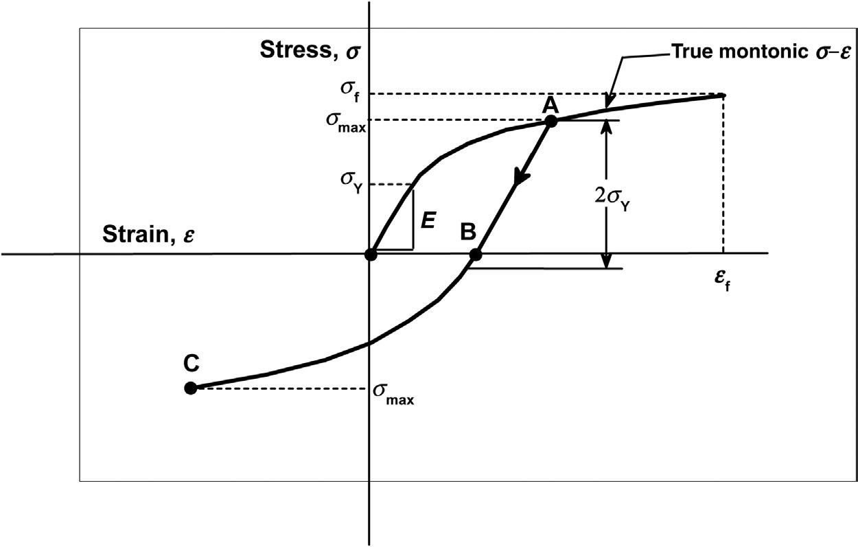
When the stress–strain measurement shown in Fig. 1.26 is reversed at a point after the yield stress, σY, but before failure, εf, the stress–strain relationship will initially follow a line with a slope equivalent to the elastic modulus E. This is illustrated by segment A–B in Fig. 1.28. If the process were stopped at point B, the length of the specimen does not fully recover to its initial value. However, in this particular example the specimen is then subjected to a compressive load to σ max to point C in Fig. 1.28.
where RA, (A0 Af)/A0 (the reduction in crosssectional area of the specimen).
Fig. 1.26 has a region labeled the elastic region. This region of the stress–strain curve is linear. In this region, ideally, if the stress is removed, the strain returns back to zero. The deformation is completely reversible. The modulus of elasticity or Young’s modulus is defined by the slope of the stress–strain curve in the elastic region. The end point of the linear elastic region is called the yield point or elastic limit. The stress at the yield point is called the yield stress, σY The rest of the stress–strain curve beyond the elastic region is called the plastic region. The total true strain is calculated from the equations given earlier. The true stress–strain curve shown in Fig. 1.26 can be approximately modeled by Eq. (1.18):
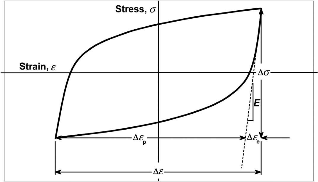
If the loading process shown in Fig. 1.28 is reversed again from σ max to +σmax, then a hysteresis loop will result such as that shown in Fig. 1.29. The hysteresis loop defines a single fatigue cycle in the strain–life method. After a number of cycles the hysteresis loop stabilizes. The stability occurs normally in less than 10% of the total life. The hysteresis loop is often characterized by its stress range, ∆σ, and strain range, ∆ε. The strain range may be split into an elastic part, ∆εe, and a plastic part, ∆ε p
When subjected to strain-controlled cyclic loading, the stress–strain response of a material can change depending on the number of applied cycles. In plastics, the maximum stress generally decreases with the increase in the number of cycles. The test is typically run to failure of the specimen or some maximum number of cycles, often 1 × 10⁷ cycles.
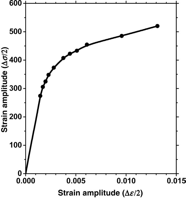
The test is often run at a series of different strain ranges (or strain amplitudes) on new specimens. Each strain range tested will have a corresponding
Figure 1.27 Necking in a plastic specimen at failure.
stress range that is measured. These data can be plotted as shown in Fig. 1.30 and the result is called a cyclic stress–strain curve.
The cyclic stress–strain curve is different from the initial behavior that is measured in a traditional tensile test. A power function (Eq. (1.19)) may be fit to this curve to obtain three material properties:
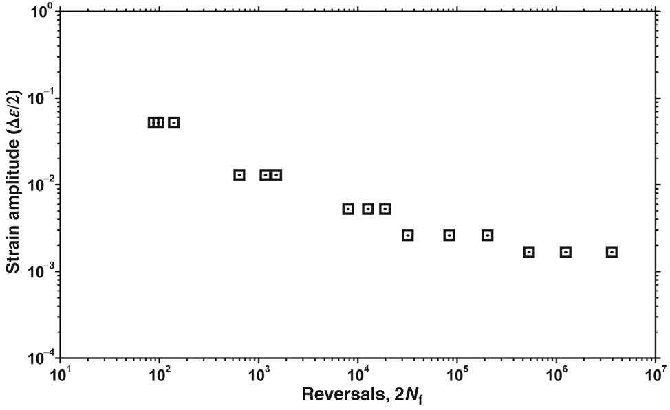
done with machines that control the strain. The strain range is controlled and the corresponding stress range and fatigue life are measured. When a series of these cyclic stress–strain measurements (to failure) are done at different strain levels, the data may be plotted as shown in Fig. 1.31. The data are usually plotted on a log–log plot, with reversals (note: 2 reversals = 1 cycle) or cycles to failure on the X-axis and strain amplitude on the Y-axis. As can be deduced from this plot the data are usually run in duplicate or triplicate at each set strain amplitude.
where K9, cyclic strength coefficient; n 9, cyclic strain hardening exponent; E, elastic modulus.
1.3.3 Strain–Life Behavior
The cyclic stress–strain measurement can be run until the specimen fails or until a maximum number of cycles have been made. These measurements are
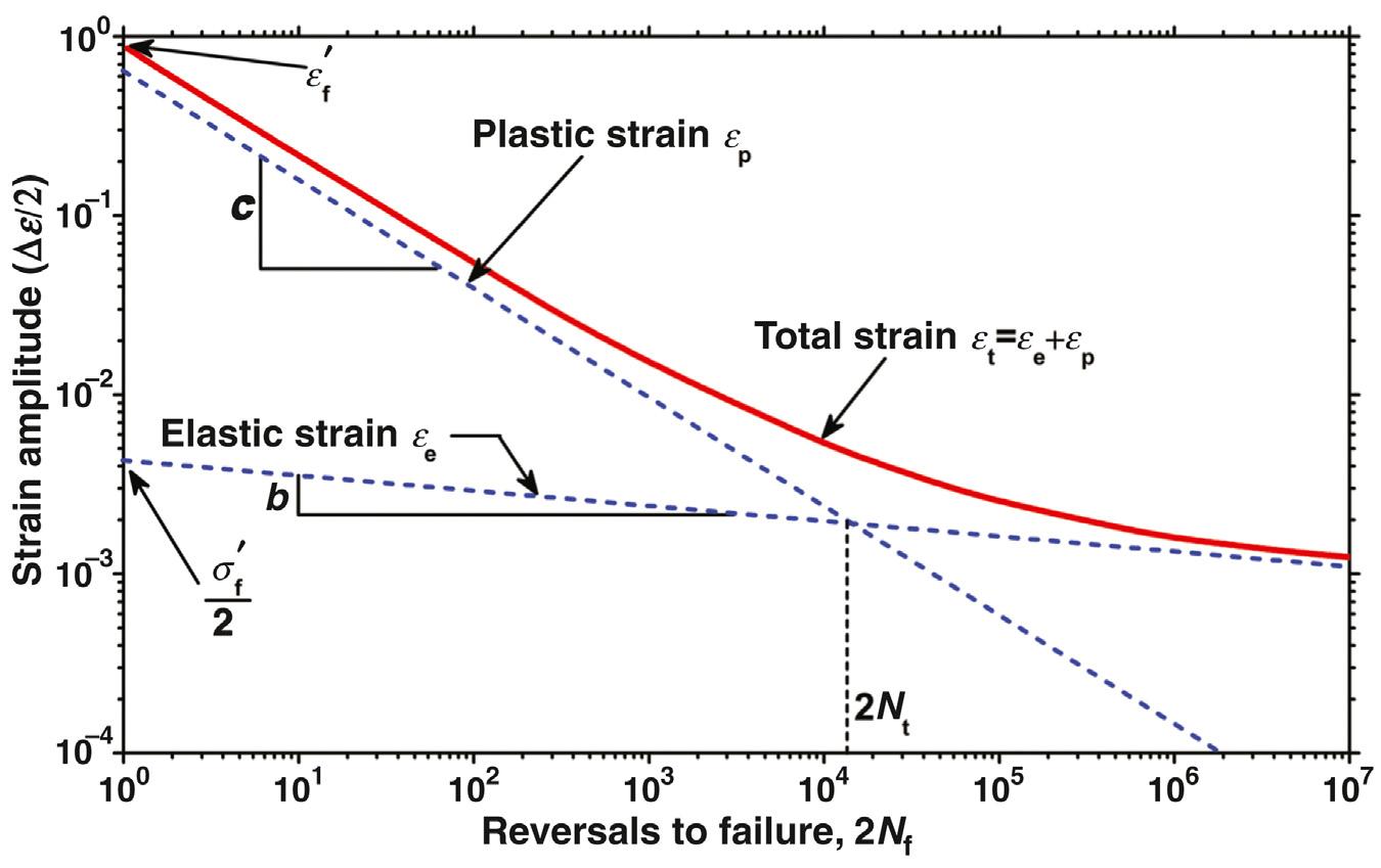
Separate researchers had noticed that the lowercycle data points could be fit by a straight line and the higher-cycle points could be fit by separate straight lines as shown in Fig. 1.32 [7–9].
Figure 1.28 Stress–strain behavior after a reversal.
Figure 1.29 Stress–strain behavior after a second reversal. Figure 1.30 A cyclic stress–strain curve.
The equation developed for the high-cycle straight line on the log–log strain–life plot corresponds to elastic material behavior of the material. The equation developed, shown in Eq. (1.20), defines two material parametersa:
where εp, the plastic component of the cyclic strain amplitude; ε′ f , the fatigue ductility coefficient; Nf, number of cycles to failure; c, the fatigue ductility exponent.
The complete strain–life curve, εt, is the sum of the elastic and plastic components (Eq. (1.22)):
All of this is summarized in Fig. 1.32.
One additional parameter shown on this graph is the transition life, 2Nt. This represents the life at which the elastic and plastic strain ranges are equivalent and can be expressed by Eq. (1.23). The transition life provides an accepted demarcation between low-cycle fatigue (LCF) and high-cycle fatigue (HCF) regimes.
where εe, the elastic component of the cyclic strain amplitude; E, elastic modulus; σa, cyclic stress amplitude; σ ′ f , the fatigue strength coefficient; Nf, number of cycles to failure; b, the fatigue strength exponent.
The equation developed for the low-cycle straight line on the log–log strain–life plot corresponds to plastic material behavior of the material. The equation developed, shown in Eq. (1.21), defines two material parameters [4,5]:
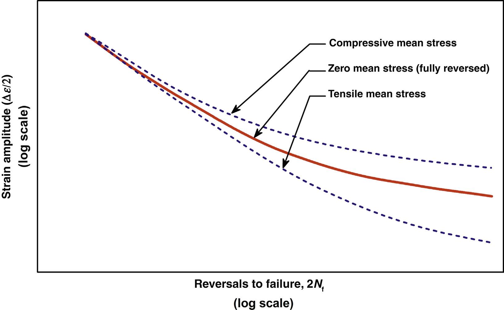
While fatigue data collected in the laboratory are generated using a fully reversed stress cycle, actual loading applications usually involve a nonzero mean stress. The mean stress can be compressive or zero and it affects the strain–life curve as shown schematically in Fig. 1.33. Mean stress has its largest effects in the high-cycle regime. Compressive means extend life and tensile means reduce it.
Figure 1.32 A strain–life curve modeled.
Figure 1.31 A strain–life plot.
1.33 The effect of mean stress on the strain–life curve.
1.3.4 Stress–Life Behavior
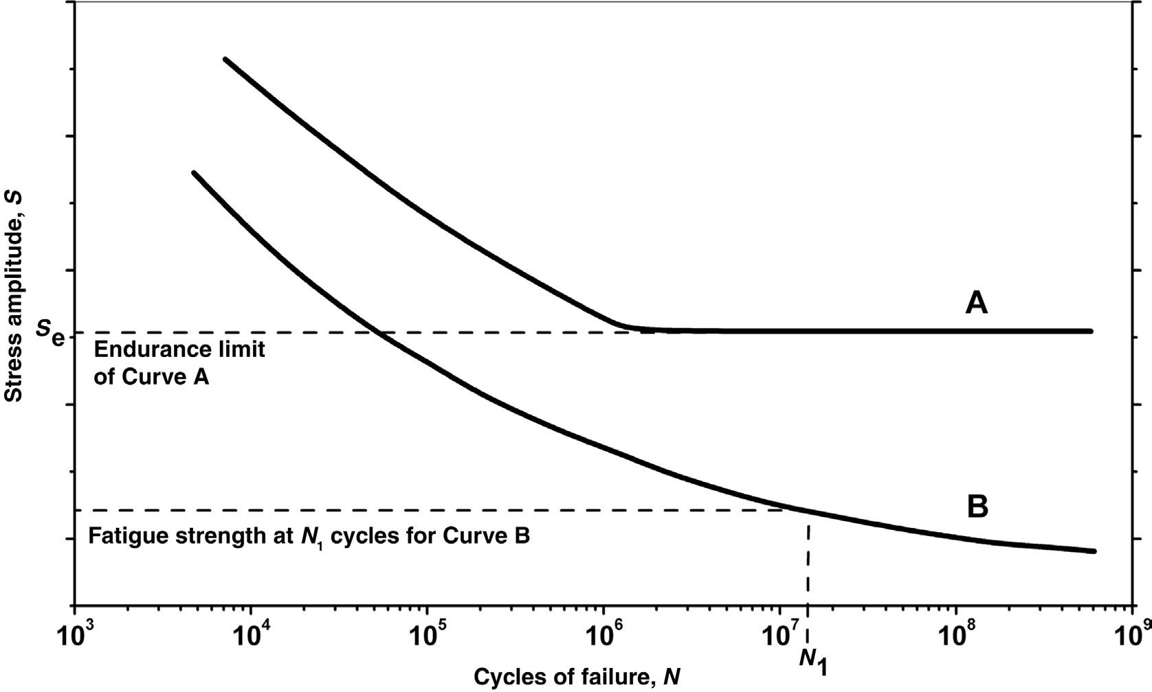
The most common published fatigue data chart is the stress–life curve which is commonly called an S–N curve or a Wöhler [10] curve. This is a graph of the magnitude of a cyclic stress (S), linear or log scale, against the cycles to failure (N) on a log scale. The cyclic measurement is made under constant oscillatory
load amplitude. It is generally applied in high-cycle regimes, whereas the strain–life behavior is used in low-cycle regimes. Fig. 1.34 shows two generic S–N curves. Curve A in this figure shows a fatigue limit. If the material is loaded below the fatigue limit, it will not fail, regardless of the number of fatigue cycles it experiences. Many materials do not behave in this manner and their S–N curve will look more like Curve
1.34 Two typical stress–life curves.
Figure
Figure
B in Fig. 1.34 Fatigue strength is noted on this curve and is defined as the stress amplitude at which failure occurs for a given number of cycles. Inversely, fatigue life is the number of cycles required for a material to fail at a given stress amplitude.
For those fatigue-tested specimens that survive the test through the maximum specified cycle limit without failure, the fatigue damage may still be estimated. The short-term properties may be measured on these specimens (eg, tensile strength and elongation at break). The ratio of the short-term properties of new (untested) specimens to those of the tested specimens constitutes a measure of the damage suffered in the fatigue test.
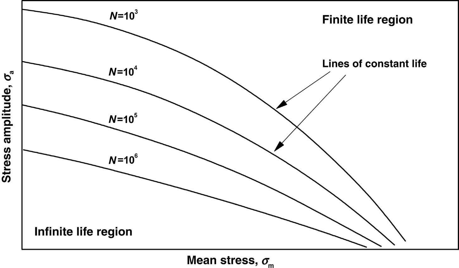
Most S–N curves are run at zero mean stress. When the fatigue tests are run at a nonzero mean stress, a different plot called a Haigh diagram is often made. The Haigh diagram, as shown in Fig. 1.35, plots the mean stress on the X-axis versus the stress amplitude on the Y-axis. A family of curves is typical with lines drawn at a given life. The region under the lowest curve is called the infinite life region. The finite life region is the region above the curves.
1.4 Fatigue Process
Failure by fatigue always involves cracking [11,12]. The process may be simplified into three steps:
1. crack initiation or nucleation
2. crack growth or propagation
3. final fracture
1.4.1 Crack Initiation
The initial crack occurs in this stage. The crack may be caused by:
1. cyclic loading;
2. surface scratches induced during handling or tooling of the material;
3. a defect introduced during manufacture, such as during casting or molding;
4. mechanical impact;
5. thermal shock, thermal expansion or contraction;
6. chemical attack (eg, pitting or corrosion).
1.4.2 Crack Growth or Propagation
Once a crack has started, it continues to grow as a result of continuously applied stresses present under the influence of cyclic loading. The crack will grow to a critical length, and then fracture of the component will occur. The rate of the crack growth before it reaches the critical length directly influences fatigue life. Fortunately a mathematical model known as Paris Law [13] provides a way to predict the crack growth rate.
The stress intensity factor, K, is used in fracture mechanics to accurately predict the stress intensity near the tip of a crack in an item caused by a load applied someplace on that item or by residual stresses. The magnitude of K depends on sample geometry, the size and location of the crack, and the magnitude and
Figure 1.35 A gener ic Haigh diagram.
the distribution of loads on the material. Eq. (1.24) shows the calculation of the stress intensity factor:
σπ = KY a (1.24)
where Y, dimensionless parameter used to account for geometry; σ, uniform tensile stress perpendicular to the plane of the crack; a, the crack size.
Stress intensity factors have been tabulated for thousands of part and crack geometries [14]
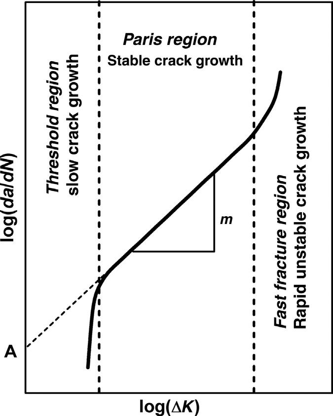
Paris proposed that the stress intensity factor range, ∆K, characterizes subcritical crack growth under fatigue loading, because he found that plots of crack growth rate versus stress intensity factor range gave straight lines on log–log scales. The stress intensity factor range is defined by Eq. (1.25):
σπ ∆= ∆ KY a (1.25)
The equation of that line is shown in Eq. (1.26), where C and m are constants for a given material. Eq. (1.26) can be rearranged to remove the logs giving Eq. (1.27):
1.36 A crack growth graph showing three regions.
occurs when the material that has not been affected by the crack cannot withstand the applied stress. This stage happens very quickly. Failure in materials is often classified as ductile or brittle. Brittle failure occurs in some metals, which experience little or no plastic deformation prior to fracture. Ductile failure shows observable plastic deformation prior to fracture. At times materials behave in a transitional manner—partially ductile/brittle.
Integrating this equation from zero to the number of cycles which caused fast fracture, or from initial and final crack size, gives Eq. (1.28), which became known as the Paris Law:
It was later realized that the Paris Law applied to growth rates in a particular range as shown in Fig. 1.36. This figure, a fatigue crack growth rate curve, plots the fatigue crack growth rate against the stress intensity factor range. The lower crack growth rate region is called the threshold regime. The higher growth rate regime occurs where values of maximum stress intensity in the fatigue cycle and failure approached rapidly. More details are available in the literature [15].
1.4.3 Failure
As the crack grows there is less material available to withstand the applied stress or strain. Failure
Fatigue failure is often classified into two types, HCF and LCF. High-cycle failure is generally classified as failure above 104 cycles. In HCF situations, material performance is commonly characterized by the S–N curve described in the previous section.
Where the stress is high enough for plastic deformation to occur leading to failure in less than 104 cycles, LCF is usually characterized by the Coffin–Manson relation [16,17] given in Eq. (1.29):
where ∆εp/2, the plastic strain amplitude; ε′ f , the fatigue ductility coefficient, the failure strain for a single reversal; 2N, the number of reversals to failure; c, the fatigue ductility exponent.
Examination of the fracture site of material failed by fatigue often shows two distinct regions. One region is smooth or burnished as a result of the rubbing of the bottom and top of the crack during the cyclic action of the stress or strain. The second region appears granular, due to the rapid failure of the material. These may be seen in Fig. 1.37. The rough,
Figure