

https://ebookmass.com/product/applied-statistics-theory-andproblem-solutions-with-r-dieter-rasch-rostock/
Instant digital products (PDF, ePub, MOBI) ready for you
Download now and discover formats that fit your needs...
Applied Statistics with R: A Practical Guide for the Life Sciences Justin C. Touchon
https://ebookmass.com/product/applied-statistics-with-r-a-practicalguide-for-the-life-sciences-justin-c-touchon/ ebookmass.com
Applied Statistics for Environmental Science With R 1st Edition Abbas F. M. Alkarkhi
https://ebookmass.com/product/applied-statistics-for-environmentalscience-with-r-1st-edition-abbas-f-m-alkarkhi/
ebookmass.com
Applied Univariate, Bivariate, and Multivariate Statistics: Understanding Statistics for Social and Natural Scientists, With Applications in SPSS and R 2nd Edition Daniel J. Denis
https://ebookmass.com/product/applied-univariate-bivariate-andmultivariate-statistics-understanding-statistics-for-social-andnatural-scientists-with-applications-in-spss-and-r-2nd-edition-danielj-denis/ ebookmass.com
Family in Transition 17th Edition, (Ebook PDF)
https://ebookmass.com/product/family-in-transition-17th-edition-ebookpdf/
ebookmass.com


Silas: Club Sin Book 4 Jasinda Wilder
https://ebookmass.com/product/silas-club-sin-book-4-jasinda-wilder/
ebookmass.com
Islam and Muslim Resistance to Modernity in Turkey 1st ed. 2020 Edition Gokhan Bacik
https://ebookmass.com/product/islam-and-muslim-resistance-tomodernity-in-turkey-1st-ed-2020-edition-gokhan-bacik/
ebookmass.com
Infinity, Causation, and Paradox Alexander R Pruss


https://ebookmass.com/product/infinity-causation-and-paradoxalexander-r-pruss/
ebookmass.com
Research Methods, Statistics, and Applications Second Edition – Ebook PDF Version
https://ebookmass.com/product/research-methods-statistics-andapplications-second-edition-ebook-pdf-version/
ebookmass.com
Principles of Computer Security - Wm. Arthur Conklin & Greg White & Chuck Cothren & Roger L. Davis & Dwayne Williams
https://ebookmass.com/product/principles-of-computer-security-wmarthur-conklin-greg-white-chuck-cothren-roger-l-davis-dwayne-williams/
ebookmass.com

https://ebookmass.com/product/lead-book-1-gregory-h-garrison/

ebookmass.com
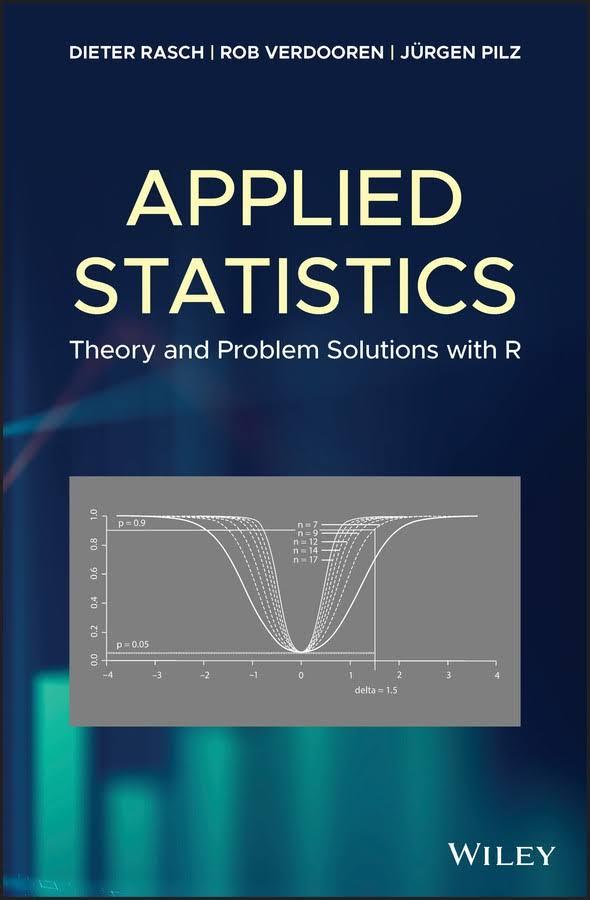
AppliedStatistics
AppliedStatistics
TheoryandProblemSolutionswithR
DieterRasch
Rostock
Germany
RobVerdooren
Wageningen
TheNetherlands
JürgenPilz
Klagenfurt
Austria
Thiseditionfirstpublished2020
©2020JohnWiley&SonsLtd
Allrightsreserved.Nopartofthispublicationmaybereproduced,storedinaretrievalsystem,or transmitted,inanyformorbyanymeans,electronic,mechanical,photocopying,recordingorotherwise, exceptaspermittedbylaw.Adviceonhowtoobtainpermissiontoreusematerialfromthistitleisavailable athttp://www.wiley.com/go/permissions.
TherightofDieterRasch,RobVerdoorenandJürgenPilztobeidentifiedastheauthorsofthisworkhas beenassertedinaccordancewithlaw.
RegisteredOffices
JohnWiley&Sons,Inc.,111RiverStreet,Hoboken,NJ07030,USA
JohnWiley&SonsLtd,TheAtrium,SouthernGate,Chichester,WestSussex,PO198SQ,UK
EditorialOffice
9600GarsingtonRoad,Oxford,OX42DQ,UK
Fordetailsofourglobaleditorialoffices,customerservices,andmoreinformationaboutWileyproducts visitusatwww.wiley.com.
Wileyalsopublishesitsbooksinavarietyofelectronicformatsandbyprint-on-demand.Somecontentthat appearsinstandardprintversionsofthisbookmaynotbeavailableinotherformats.
LimitofLiability/DisclaimerofWarranty
Whilethepublisherandauthorshaveusedtheirbesteffortsinpreparingthiswork,theymakeno representationsorwarrantieswithrespecttotheaccuracyorcompletenessofthecontentsofthisworkand specificallydisclaimallwarranties,includingwithoutlimitationanyimpliedwarrantiesofmerchantabilityor fitnessforaparticularpurpose.Nowarrantymaybecreatedorextendedbysalesrepresentatives,written salesmaterialsorpromotionalstatementsforthiswork.Thefactthatanorganization,website,orproductis referredtointhisworkasacitationand/orpotentialsourceoffurtherinformationdoesnotmeanthatthe publisherandauthorsendorsetheinformationorservicestheorganization,website,orproductmayprovide orrecommendationsitmaymake.Thisworkissoldwiththeunderstandingthatthepublisherisnotengaged inrenderingprofessionalservices.Theadviceandstrategiescontainedhereinmaynotbesuitableforyour situation.Youshouldconsultwithaspecialistwhereappropriate.Further,readersshouldbeawarethat websiteslistedinthisworkmayhavechangedordisappearedbetweenwhenthisworkwaswrittenandwhen itisread.Neitherthepublishernorauthorsshallbeliableforanylossofprofitoranyothercommercial damages,includingbutnotlimitedtospecial,incidental,consequential,orotherdamages.
LibraryofCongressCataloging-in-PublicationData
Names:Rasch,Dieter,author.|Verdooren,L.R.,author.|Pilz,Jürgen, 1951-author.
Title:Appliedstatistics:theoryandproblemsolutionswithR/Dieter Rasch(Rostock,GM),RobVerdooren,JürgenPilz.
Description:Hoboken,NJ:Wiley,2020.|Includesbibliographicalreferences andindex.|
Identifiers:LCCN2019016568(print)|LCCN2019017761(ebook)|ISBN 9781119551553(AdobePDF)|ISBN9781119551546(ePub)|ISBN9781119551522 (hardcover)
Subjects:LCSH:Mathematicalstatistics–Problems,exercises,etc.|R (Computerprogramlanguage)
Classification:LCCQA276(ebook)|LCCQA276.R36682019(print)|DDC 519.5–dc23
LCrecordavailableathttps://lccn.loc.gov/2019016568
Coverdesign:Wiley
CoverImages:©DieterRasch,©whiteMocca/Shutterstock
Setin10/12ptWarnockProbySPiGlobal,Chennai,India
Contents
Preface xi
1The R-Package,SamplingProcedures,andRandomVariables 1
1.1Introduction 1
1.2TheStatisticalSoftwarePackage R 1
1.3SamplingProceduresandRandomVariables 4 References 10
2PointEstimation 11
2.1Introduction 11
2.2EstimatingLocationParameters 12
2.2.1MaximumLikelihoodEstimationofLocationParameters 17
2.2.2EstimatingExpectationsfromCensoredSamplesandTruncated Distributions 20
2.2.3EstimatingLocationParametersofFinitePopulations 23
2.3EstimatingScaleParameters 24
2.4EstimatingHigherMoments 27
2.5ContingencyTables 29
2.5.1ModelsofTwo-DimensionalContingencyTables 29
2.5.1.1ModelI 29
2.5.1.2ModelII 29
2.5.1.3ModelIII 30
2.5.2AssociationCoefficientsfor2 × 2Tables 30 References 38
3TestingHypotheses–One-andTwo-SampleProblems 39
3.1Introduction 39
3.2TheOne-SampleProblem 41
3.2.1TestsonanExpectation 41
3.2.1.1TestingtheHypothesisontheExpectationofaNormalDistribution withKnownVariance 41
3.2.1.2TestingtheHypothesisontheExpectationofaNormalDistribution withUnknownVariance 47
3.2.2TestontheMedian 51
3.2.3TestontheVarianceofaNormalDistribution 54
3.2.4TestonaProbability 56
3.2.5PairedComparisons 57
3.2.6SequentialTests 59
3.3TheTwo-SampleProblem 63
3.3.1TestsonTwoExpectations 63
3.3.1.1TheTwo-Sample t -Test 63
3.3.1.2TheWelchTest 66
3.3.1.3TheWilcoxonRankSumTest 70
3.3.1.4DefinitionofRobustnessandResultsofComparingTestsbySimulation 72
3.3.1.5SequentialTwo-SampleTests 74
3.3.2TestonTwoMedians 76
3.3.2.1Rationale 77
3.3.3TestonTwoProbabilities 78
3.3.4TestsonTwoVariances 79 References 81
4ConfidenceEstimations–One-andTwo-SampleProblems 83
4.1Introduction 83
4.2TheOne-SampleCase 84
4.2.1AConfidenceIntervalfortheExpectationofaNormalDistribution 84
4.2.2AConfidenceIntervalfortheVarianceofaNormalDistribution 91
4.2.3AConfidenceIntervalforaProbability 93
4.3TheTwo-SampleCase 96
4.3.1AConfidenceIntervalfortheDifferenceofTwoExpectations–Equal Variances 96
4.3.2AConfidenceIntervalfortheDifferenceofTwoExpectations–Unequal Variances 98
4.3.3AConfidenceIntervalfortheDifferenceofTwoProbabilities 100 References 104
5AnalysisofVariance(ANOVA)–FixedEffectsModels 105
5.1Introduction 105
5.1.1RemarksaboutProgramPackages 106
5.2PlanningtheSizeofanExperiment 106
5.3One-WayAnalysisofVariance 108
5.3.1AnalysingObservations 109
5.3.2DeterminationoftheSizeofanExperiment 112
5.4Two-WayAnalysisofVariance 115
5.4.1Cross-Classification(A × B) 115
5.4.1.1ParameterEstimation 117
5.4.1.2TestingHypotheses 119
5.4.2NestedClassification(A≻B) 131
5.5Three-WayClassification 134
5.5.1CompleteCross-Classification(A×B × C ) 135
5.5.2NestedClassification(C ≺ B ≺ A) 144
5.5.3MixedClassifications 147
5.5.3.1Cross-ClassificationbetweenTwoFactorswhereOneofThemIs Sub-OrdinatedtoaThirdFactor((B ≺ A)xC ) 148
5.5.3.2Cross-ClassificationofTwoFactors,inwhichaThirdFactorisNested (C ≺ (A × B)) 153 References 157
6AnalysisofVariance–ModelswithRandomEffects 159
6.1Introduction 159
6.2One-WayClassification 159
6.2.1EstimationoftheVarianceComponents 160
6.2.1.1ANOVAMethod 160
6.2.1.2MaximumLikelihoodMethod 164
6.2.1.3 REML –Estimation 166
6.2.2TestsofHypothesesandConfidenceIntervals 169
6.2.3ExpectationandVariancesoftheANOVAEstimators 174
6.3Two-WayClassification 176
6.3.1Two-WayCrossClassification 176
6.3.2Two-WayNestedClassification 182
6.4Three-WayClassification 186
6.4.1Three-WayCross-ClassificationwithEqualSub-ClassNumbers 186
6.4.2Three-WayNestedClassification 192
6.4.3Three-WayMixedClassifications 195
6.4.3.1Cross-ClassificationBetweenTwoFactorsWhereOneofThemis Sub-OrdinatedtoaThirdFactor((B ≺ A)×C ) 195
6.4.3.2Cross-ClassificationofTwoFactorsinWhichaThirdFactorisNested (C ≺ (A×B)) 197 References 199
7AnalysisofVariance–MixedModels 201
7.1Introduction 201
7.2Two-WayClassification 201
7.2.1BalancedTwo-WayCross-Classification 201
7.2.2Two-WayNestedClassification 214
7.3Three-WayLayout 223
7.3.1Three-WayAnalysisofVariance–Cross-Classification A × B × C223
7.3.2Three-WayAnalysisofVariance–NestedClassification A ≻ B ≻ C230
7.3.2.1Three-WayAnalysisofVariance–NestedClassification–ModelIII–BalancedCase 230
7.3.2.2Three-WayAnalysisofVariance–NestedClassification–ModelIV–BalancedCase 232
7.3.2.3Three-WayAnalysisofVariance–NestedClassification–ModelV–BalancedCase 234
7.3.2.4Three-WayAnalysisofVariance–NestedClassification–ModelVI–BalancedCase 236
7.3.2.5Three-WayAnalysisofVariance–NestedClassification–ModelVII–BalancedCase 237
7.3.2.6Three-WayAnalysisofVariance–NestedClassification–ModelVIII–BalancedCase 238
7.3.3Three-WayAnalysisofVariance–MixedClassification–(A × B) ≻ C239
7.3.3.1Three-WayAnalysisofVariance–MixedClassification–(A × B) ≻ C ModelIII 239
7.3.3.2Three-WayAnalysisofVariance–MixedClassification–(A × B) ≻ C ModelIV 242
7.3.3.3Three-WayAnalysisofVariance–MixedClassification–(A × B) ≻ C ModelV 243
7.3.3.4Three-WayAnalysisofVariance–MixedClassification–(A × B) ≻ C ModelVI 245
7.3.4Three-WayAnalysisofVariance–MixedClassification–(A ≻ B) × C247
7.3.4.1Three-WayAnalysisofVariance–MixedClassification–(A ≻ B) × C ModelIII 247
7.3.4.2Three-WayAnalysisofVariance–MixedClassification–(A ≻ B) × C ModelIV 249
7.3.4.3Three-WayAnalysisofVariance–MixedClassification–(A ≻ B) × C ModelV 251
7.3.4.4Three-WayAnalysisofVariance–MixedClassification–(A ≻ B) × C ModelVI 253
7.3.4.5Three-WayAnalysisofVariance–MixedClassification–(A ≻ B) × C modelVII 254
7.3.4.6Three-WayAnalysisofVariance–MixedClassification–(A ≻ B) × C ModelVIII 255 References 256
8RegressionAnalysis 257
8.1Introduction 257
8.2RegressionwithNon-RandomRegressors–ModelIofRegression 262
8.2.1LinearandQuasilinearRegression 262
8.2.1.1ParameterEstimation 263
8.2.1.2ConfidenceIntervalsandHypothesesTesting 274
8.2.2IntrinsicallyNon-LinearRegression 282
8.2.2.1TheAsymptoticDistributionoftheLeastSquaresEstimators 283
8.2.2.2TheMichaelis–MentenRegression 285
8.2.2.3ExponentialRegression 290
8.2.2.4TheLogisticRegression 298
8.2.2.5TheBertalanffyFunction 306
8.2.2.6TheGompertzFunction 312
8.2.3OptimalExperimentalDesigns 315
8.2.3.1SimpleLinearandQuasilinearRegression 316
8.2.3.2IntrinsicallyNon-linearRegression 317
8.2.3.3TheMichaelis-MentenRegression 319
8.2.3.4ExponentialRegression 319
8.2.3.5TheLogisticRegression 320
8.2.3.6TheBertalanffyFunction 321
8.2.3.7TheGompertzFunction 321
8.3ModelswithRandomRegressors 322
8.3.1TheSimpleLinearCase 322
8.3.2TheMultipleLinearCaseandtheQuasilinearCase 330
8.3.2.1HypothesesTesting-General 333
8.3.2.2ConfidenceEstimation 333
8.3.3TheAllometricModel 334
8.3.4ExperimentalDesigns 335 References 335
9AnalysisofCovariance(ANCOVA) 339
9.1Introduction 339
9.2CompletelyRandomisedDesignwithCovariate 340
9.2.1BalancedCompletelyRandomisedDesign 340
9.2.2UnbalancedCompletelyRandomisedDesign 350
9.3RandomisedCompleteBlockDesignwithCovariate 358
9.4ConcludingRemarks 365 References 366
10MultipleDecisionProblems 367
10.1Introduction 367
10.2SelectionProcedures 367
10.2.1TheIndifferenceZoneFormulationforSelectingExpectations 368
10.2.1.1IndifferenceZoneSelection, �� 2 Known 368
10.2.1.2IndifferenceZoneSelection, �� 2 Unknown 371
10.3TheSubsetSelectionProcedureforExpectations 371
10.4OptimalCombinationoftheIndifferenceZoneandtheSubsetSelection Procedure 372
10.5SelectionoftheNormalDistributionwiththeSmallestVariance 375 10.6MultipleComparisons 375
10.6.1TheSolutionofMCProblem10.1 377
10.6.1.1The F -testforMCProblem10.1 377
10.6.1.2Scheffé’sMethodforMCProblem10.1 378
10.6.1.3Bonferroni’sMethodforMCProblem10.1 379
10.6.1.4Tukey’sMethodforMCProblem10.1for ni = n382
10.6.1.5GeneralisedTukey’sMethodforMCProblem10.1for ni ≠ n383
10.6.2TheSolutionofMCProblem10.2–theMultiplet-Test 384
10.6.3TheSolutionofMCProblem10.3–PairwiseandSimultaneous ComparisonswithaControl 385
10.6.3.1PairwiseComparisons–TheMultiplet-Test 385 10.6.3.2SimultaneousComparisons–TheDunnettMethod 387 References 390
11GeneralisedLinearModels 393
11.1Introduction 393
11.2ExponentialFamiliesofDistributions 394
11.3GeneralisedLinearModels–AnOverview 396
11.4Analysis–FittingaGLM–TheLinearCase 398
x Contents
11.5BinaryLogisticRegression 399
11.5.1Analysis 400
11.5.2Overdispersion 408
11.6PoissonRegression 411
11.6.1Analysis 411
11.6.2Overdispersion 417
11.7TheGammaRegression 417
11.8GLMforGammaRegression 418
11.9GLMfortheMultinomialDistribution 425 References 428
12SpatialStatistics 429
12.1Introduction 429
12.2Geostatistics 431
12.2.1Semi-variogramFunction 432
12.2.2Semi-variogramParameterEstimation 439
12.2.3Kriging 440
12.2.4 Trans-GaussianKriging 446
12.3SpecialProblemsandOutlook 450
12.3.1GeneralisedLinearModelsinGeostatistics 450
12.3.2CopulaBasedGeostatisticalPrediction 451 References 451
AppendixAListofProblems 455
AppendixBSymbolism 483
AppendixCAbbreviations 485
AppendixDProbabilityandDensityFunctions 487
Index 489
Preface
Wewrotethisbookforpeoplethathavetoapplystatisticalmethodsintheirresearch butwhosemaininterestisnotintheoremsandproofs.Becauseofsuchanapproach, ouraimisnottoprovidethedetailedtheoreticalbackgroundofstatisticalprocedures. Whilemathematicalstatisticsasabranchofmathematicsincludesdefinitionsaswellas theoremsandtheirproofs,appliedstatisticsgiveshintsfortheapplicationoftheresults ofmathematicalstatistics.
Sometimesappliedstatisticsusessimulationresultsinplaceofresultsfromtheorems. Anexampleisthatthenormalityassumptionneededformanytheoremsinmathematicalstatisticscanbeneglectedinapplicationsforlocationparameterssuchas theexpectation,seeforthisRaschandTiku(1985).Nearlyallstatisticaltestsand confidenceestimationsforexpectationshavebeenshownbysimulationstobevery robustagainsttheviolationofthenormalityassumptionneededtoprovecorresponding theorems.
WegavethepresentbookananalogousstructuretothatofRaschandSchott(2018)so thatthereadercaneasilyfindthecorrespondingtheoreticalbackgroundthere.Chapter 11‘GeneralisedLinearModels’andChapter12‘SpatialStatistics’ofthepresentbook havenoprototypeinRaschandSchott(2018).Further,thepresentbookcontainsno exercises;lecturerscaneitherusetheexercises(withsolutionsintheappendix)inRasch andSchott(2018)ortheexercisesintheproblemsmentionedbelow.
Instead,ouraimwastodemonstratethetheorypresentedinRaschandSchott(2018) andthatunderlyingthenewChapters11and12usingfunctionsandproceduresavailableinthestatisticalprogrammingsystemR,whichhasbecomethegoldenstandard whenitcomestostatisticalcomputing.
Withinthetext,thereaderfindsoftenthesequenceproblem–solution–example withproblemsnumberedwithinthechapters.Readersinterestedonlyinspecialapplicationsinmanycasesmayfindthecorrespondingprocedureinthelistofproblemsin AppendixA.
WethankAlisonOliver(Wiley,Oxford)andMustaqAhamed(Wiley)fortheirassistanceinpublishingthisbook.
Weareveryinterestedinthecommentsofreaders.Pleasecontact: d_rasch@t-online.de,l.r.verdooren@hetnet.nl,juergen.pilz@aau.at. Rostock,Wageningen,andKlagenfurt,June2019,theauthors.
xii Preface
References
Rasch,D.andTiku,M.L.(eds.)(1985).Robustnessofstatisticalmethodsand nonparametricstatistics.In: ProceedingsoftheConferenceonRobustnessofStatistical MethodsandNonparametricStatistics,heldatSchwerin(DDR),May29-June2,1983. Boston,Lancaster,Tokyo:ReidelPubl.Co.Dordrecht.
Rasch,D.andSchott,D.(2018). MathematicalStatistics.Oxford:Wiley.
The R-Package,SamplingProcedures,andRandomVariables
1.1Introduction
Inthischapterwegiveanoverviewofthesoftwarepackage R andintroducebasic knowledgeaboutrandomvariablesandsamplingprocedures.
1.2TheStatisticalSoftwarePackage R
Inpracticalinvestigations,professionalstatisticalsoftwareisusedtodesign experimentsortoanalysedataalreadycollected.Weapplyherethesoftwarepackage R. Anybodycanextendthefunctionalityof R withoutanyrestrictionsusingfreesoftware tools;moreover,itisalsopossibletoimplementspecialstatisticalmethodsaswell ascertainproceduresofCandFORTRAN.Suchtoolsareofferedontheinternetin standardisedarchives.ThemostpopulararchiveisprobablyCRAN(Comprehensive R ArchiveNetwork),aservernetthatissupervisedbythe R DevelopmentCore Team.ThisnetalsooffersthepackageOPDOE(optimaldesignofexperiments), whichwasthoroughlydescribedinRasch etal .(2011).Furtheritoffersthefollowing packagesusedinthisbook: car,lme4,DunnettTests,VCA,lmerTest, mvtnorm,seqtest,faraway,MASS,glm2,geoR,gstat. Apartfromonlyafewexceptions, R containsimplementationsforallstatisticalmethodsconcerninganalysis,evaluation,andplanning.Wereferfordetailsto Crawley(2013).
Thesoftwarepackage R isavailablefreeofchargefromhttp://cran.r-project.org fortheoperatingsystemsLinux,MacOSX,andWindows.Theinstallationunder MicrosoftWindowstakesplacevia‘Windows’.Choosing‘base’theinstallationplatformisreached.Using‘DownloadR2.X.XforWindows’(Xstandsfortherequired versionnumber)thesetupfilecanbedownloaded.Afterthisfileisstartedthesetup assistantrunsthroughtheinstallationsteps.Inthisbook,allstandardsettingsare adopted.Theinterestedreaderwillfindmoreinformationabout R athttp://www.rproject.orgorinCrawley(2013).
Afterstarting R theinputwindowwillbeopened,presentingtheredcolouredinput request:‘>’.Herecommandscanbewrittenupandcarriedoutbypressingtheenter button.Theoutputisgivendirectlybelowthecommandline.However,theusercanalso realiselinechangesaswellaslineindentsforincreasingclarity.Notallthisinfluencesthe functionalprocedure.Acommandtoreadforinstancedata y = (1,3,8,11)isasfollows: AppliedStatistics:TheoryandProblemSolutionswithR, FirstEdition. DieterRasch,RobVerdooren,andJürgenPilz. ©2020JohnWiley&SonsLtd.Published2020byJohnWiley&SonsLtd.
2
1The R-Package,SamplingProcedures,andRandomVariables
>y<-c(1,3,8,11)
Theassignmentoperatorin R isthetwo-charactersequence‘<-’or‘=’.
TheWorkspaceisaspecialworkingenvironmentin R.There,certainobjectscanbe storedthatwereobtainedduringthecurrentworkwith R.Suchobjectscontainthe resultsofcomputationsanddatasets.AWorkspaceisloadedusingthemenu
File–LoadWorkspace...
Inthisbookthe R-commandsstartwith >.Readerswholiketouse R-commandsmust onlytypeorcopythetextafter > intothe R-window.
Anadvantageof R isthat,aswithotherstatisticalpackageslikeSASandIBM-SPSS,we nolongerneedanappendixwithtablesinstatisticalbooks.Oftentablesofthedensity ordistributionfunctionofthestandardnormaldistributionappearinsuchappendices. However,thevaluescanbeeasilycalculatedusing R.
ThenotationofthisandthefollowingchaptersisjustthatofRaschandSchott(2018).
Problem1.1 Calculatethevalue ��(z)ofthedensityfunctionofthestandardnormal distributionforagivenvalue z.
Solution
Usethecommand > dnorm(z,mean = 0,sd = 1). Ifthe mean or sd isnot specifiedtheyassumethedefaultvaluesof0and1,respectively.Hence > dnorm(z) canbeusedinProblem1.1.
Example
Wecalculatethevalue ��(1)ofthedensityfunctionofthestandardnormaldistribution using
>dnorm(1)
[1]0.2419707
Problem1.2 Calculatethevalue ��(z)ofthedistributionfunctionofthestandardnormaldistributionforagivenvalue z
Solution
Usethecommand > pnorm(z,mean = 0,sd = 1).
Example
Wecalculatethevalue ��(1)ofthedistributionfunctionofthestandardnormaldistributionby > pnorm(1,mean = 0,sd = 1) orusingthedefaultvaluesusing > pnorm(1).
>pnorm(1) [1]0.8413447
Also,forothercontinuousdistributions,weobtainusing d withthe R-nameofadistribution,thevalueofthedensityfunctionand,using p withthe R-nameofadistribution, thevalueofthedistributionfunction.Wedemonstratethisinthenextproblemforthe lognormaldistribution.
Problem1.3 Calculatethevalueofthedensityfunctionofthelognormaldistribution whoselogarithmhasmeanequalto meanlog = 0 andstandarddeviationequalto sdlog = 1 foragivenvalue z.
Solution
Usethecommand > dlnorm(z,meanlog = 0,sdlog = 1) orusethedefault values meanlog = 0 and sdlog = 1 using > dlnorm(z) .
Example
Wecalculatethevalueofthedensityfunctionofthelognormaldistributionwith meanlog = 0 and sdlog = 1 using >dlnorm(1) [1]0.3989423
Problem1.4 Calculatethevalueofthedistributionfunctionofthelognormaldistributionwhoselogarithmhasmeanequalto meanlog = 0 andstandarddeviation equalto sdlog = 1 foragivenvalue z.
Solution
Usethecommand > plnorm(z,meanlog = 0,sdlog = 1) orusethedefault values meanlog = 0 and sdlog = 1 using > plnorm(z) .
Example
Wecalculatethevalueofthedistributionfunctionforz = 1ofthelognormaldistribution with meanlog = 0 and sdlog = 1 using >plnorm(1) [1]0.5
Frommostoftheotherdistributionsweneedthequantiles(orpercentiles) qP = P ( y ≤ P ). Thiscanbedonebywriting q followedbythe R-nameofthedistribution.
Problem1.5 Calculatethe P %-quantileofthe t -distributionwithdfdegreesof freedomandoptionalnon-centralityparameterncp.
Solution
Usethecommand > qt(P,df,ncp) andforacentral t -distributionusethedefault byomitting ncp.
Example
Calculatethe95%-quantileofthecentral t -distributionwith10degreesoffreedom. >qt(0.95,10) [1]1.812461
Wedemonstratetheprocedureforthechi-squareandthe F -distribution.
Problem1.6 Calculatethe P %-quantileofthe �� 2 -distributionwithdfdegreesof freedomandoptionalnon-centralityparameterncp.
4 1The R-Package,SamplingProcedures,andRandomVariables
Solution
Usethecommand > qchisq(P,df,ncp) andforthecentral �� 2 -distributionwith dfdegreesoffreedomuse > qchisq(P,df).
Example
Calculatethe95%-quantileofthecentral �� 2 -distributionwith10degreesoffreedom.
>qchisq(0.95,10) [1]18.30704
Problem1.7 Calculatethe P%-quantileofthe F -distributionwithdf1anddf2degrees offreedomandoptionalnon-centralityparameterncp.
Solution
Usethecommand > qf(P,df1,df2,ncp),andforthecentral F -distributionwith df1anddf2degreesoffreedomuse > qf(P,df1,df2).
Example
Calculatethe95%-quantileofthe centralF -distributionwith10and20degreesof freedom!
>qf(0.95,10,20) [1]2.347878
Forthecalculationoffurthervaluesofprobabilityfunctionsofdiscreterandomvariablesorofdistributionfunctionsandquantilesthecommandscanbefoundbyusing thehelpfunctioninthetoolbarofR,andthenyoumaycallupthe‘manual’oruse Crawley(2013).
1.3SamplingProceduresandRandomVariables
Evenifwe,inthisbook,wemainlydiscusshowtoplanexperimentsandtoanalyse observeddata,westillneedbasicknowledgeaboutrandomvariablesbecause,without this,wecouldnotexplainunbiasedestimatorsortheexpectedlengthofaconfidence intervalorhowtodefinetherisksofastatisticaltests.
Definition1.1 Asamplingprocedurewithoutreplacement(wor)orwithreplacement (wr)isaruleofselectingapropersubset,namedsample,fromawell-definedfinitebasic setofobjects(population,universe).Itissaidtobeatrandomifeachelementofthe basicsethasthesameprobability p tobedrawnintothesample.Wealsocansaythat inarandomsamplingprocedureeachpossiblesamplehasthesameprobabilitytobe drawn.
A(concrete)sampleistheresultofasamplingprocedure.Samplesresultingfrom arandomsamplingprocedurearesaidtobe(concrete)randomsamplesorshortly samples.
Ifweconsiderallpossiblesamplesfromagivenfiniteuniverse,then,fromthisdefinition,itfollowsthateachpossiblesamplehasthesameprobabilitytobedrawn.
1.3SamplingProceduresandRandomVariables 5
Thereareseveralrandomsamplingproceduresthatcanbeusedinpractice.Basic setsofobjectsaremostlycalled(statistical)populationsor,synonymously,(statistical) universes.
Concerningrandomsamplingprocedures,wedistinguish(amongothercases):
• Simple(orpure)randomsamplingwithreplacement(wr)whereeachofthe N elementsofthepopulationisselectedwithprobability 1 N .
• Simplerandomsamplingwithoutreplacement(wor)whereeachunorderedsample of n differentobjectshasthesameprobabilitytobechosen.
• Inclustersampling,thepopulationisdividedintodisjointsubclasses(clusters).Randomsamplingwithoutreplacementisdoneamongtheseclusters.Intheselected clusters,allobjectsaretakenintothesample.Thiskindofselectionisoftenusedin areasampling.ItisonlyrandomcorrespondingtoDefinition1.1iftheclusterscontain thesamenumberofobjects.
• Inmulti-stagesampling,samplingisdoneinseveralsteps.Werestrictourselvestotwo stagesofsamplingwherethepopulationisdecomposedintodisjointsubsets(primary units).Partoftheprimaryunitsissampledrandomlywithoutreplacement(wor)and withinthempurerandomsamplingwithoutreplacement(wor)isdonewiththesecondaryunits.Amulti-stagesamplingisfavourableifthepopulationhasahierarchical structure(e.g.country,province,townsintheprovince).ItisatrandomcorrespondingtoDefinition1.1iftheprimaryunitscontainthesamenumberofsecondaryunits.
• Sequentialsampling,wherethesamplesizeisnotfixedatthebeginningofthesamplingprocedure.Atfirst,asmallsamplewithreplacementistakenandanalysed.Then itisdecidedwhethertheobtainedinformationissufficient,e.g.torejectortoaccept agivenhypothesis(seeChapter3),orifmoreinformationisneededbyselectinga furtherunit.
Whenaclusterorintwo-stagesamplingtheclustersorprimaryunitshavedifferent sizes(numberofelementsorareas),moresophisticatedmethodsareused(Raschetal. 2008,Methods1/31/2110,1/31/3100).
Botharandomsampling(procedure)andarbitrarysampling(procedure)canresultin thesameconcretesample.Hence,wecannotprovebyinspectingtheconcretesample itselfwhetherornotthesampleisrandomlychosen.Wehavetocheckthesampling procedureusedinstead.
Inmathematicalstatisticsrandomsamplingwithareplacementprocedureismodelledbyavector Y = (y1 , y2 , … , yn )T ofrandomvariables yi , i = 1, … , n,whichare independentlydistributedasarandomvariable y,i.e.theyallhavethesamedistribution.The yi , i = 1, , n aresaidindependentlyandidenticallydistributed(i.i.d.).This leadstothefollowingdefinition.
Definition1.2 Arandomsampleofsize n isavector Y = (y1 , y2 , … , yn )T with n i.i.d. randomvariables yi , i = 1, … , n aselements.
Randomvariablesgiveninboldprint(seeAppendixAformotivation).
Thevector Y = (y1 , y2 , … , yn )T iscalledarealisationof Y = (y1 , y2 , … , yn )T andis usedasamodelofavectorofobservedvaluesorvaluesselectedbyarandomselection procedure.
Toexplainthisapproachletusassumethatwehaveauniverseof100elements(the numbers1–100).Weliketodrawapurerandomsamplewithoutreplacement(wor)of
6
1The R-Package,SamplingProcedures,andRandomVariables
size n = 10fromthisuniverseandmodelthisby Y = (y1 , y2 , , y10 )T .Whenarandom samplehasbeendrawnitcouldbethevector Y = ( y1 , y2 , , y10 )T = (3,98,12,37,2,67, 33,21,9,56)T = (2,3,9,12,21,33,37,56,67,98)T .Thismeansthatitisonlyimportant whichelementhasbeenselectedandnotatwhichplacethishashappened.Allsamples woroccurwithprobability 1 (100 10 ) .Thedenominator (100 10 ) canbecalculatedby R withthe > choose() command
>choose(100,10) [1]1.731031e+13 andfromthistheprobabilityis 1 1731031×107 . Wecannowwrite
P {(y1 , y2 , , y10 )T =(2, 3, 9, 12, 21, 33, 37, 56, 67, 98)T }= 1 1731031 × 107
Inaprobabilitystatement,somethingmustalwaysberandom.Towrite
P {(y1 , y2 , , y10 )T =(2, 3, 9, 12, 21, 33, 37, 56, 67, 98)T } isnonsensebecause(y1 , y2 , … , y10 )T asthevectorontheright-hand-sideisavectorof specialnumbersanditisnonsensetoaskfortheprobabilitythat5equals7.
Toexplainthesituationagainweconsidertheproblemofthrowingafairdice;thisisa dicewhereweknowthateachofthenumbers1, …,6occurswiththesameprobability 1 6 .Weaskfortheprobabilitythatanevennumberisthrown.Becauseonehalfofthesix numbersareeven,thisprobabilityis 1 2 .Assumewethrowthediceusingadicecupand lettheresultbehidden,thantheprobabilityisstill 1 2 .However,ifwetakethedicecup away,arealisationoccurs,letussaya5.Now,itisstupidtoask,whatistheprobability that5isevenorthatanevennumberiseven.Probabilitystatementsaboutrealisations ofrandomvariablesaresenselessandnotallowed.Thereaderofthisbookshouldonly lookataprobabilitystatementintheformofaformulaifsomethingisinboldprint; onlyinsuchacaseisaprobabilitystatementpossible.
WelearninChapter4whataconfidenceintervalis.Itisdefinedasanintervalwith atleastonerandomboundaryandwecan,forexample,calculatewithsomesmall �� the probability1 �� thattheexpectationofsomerandomvariableiscoveredbythisinterval.However,whenwehaverealisedboundaries,thentheintervalisfixedanditeither coversordoesnotcovertheexpectation.Inappliedstatistics,weworkwithobserved datamodelledbyrealisedrandomvariables.Thenthecalculatedintervaldoesnotallow aprobabilitystatement.Wedonotknow,byusing R orotherwise,whetherthecalculated intervalcoverstheexpectationornot.Whydidwefixthisprobabilitybeforestartingthe experimentwhenwecannotuseitininterpretingtheresult?
Theanswerisnoteasy,butwewilltrytogivesomereasons.Ifaresearcherhasto carryoutmanysimilarexperimentsandineachofthemcalculatesforsomeparameter a(1 �� )confidenceinterval,thenhecansaythatinabout(1 �� )100%ofallcasesthe intervalhascoveredtheparameter,butofcoursehedoesnotknowwhenthishappened. Whatshouldwedowhenonlyoneexperimenthastobedone?Thenweshouldchoose (1 �� )solarge(say0.95or0.99)thatwecantaketheriskofmakinganerroneousstatementbysayingthattheintervalcoverstheparameter.Thisisanalogoustothesituation ofapersonwhohasaseverediseaseandneedsanoperationinhospital.Thepersoncan
1.3SamplingProceduresandRandomVariables 7
choosebetweentwohospitalsandknowsthatinhospitalAabout99%ofpeopleoperatedonsurvivedasimilaroperationandinhospitalBonlyabout80%.Ofcourse(without furtherinformation)thepersonchoosesAevenwithoutknowingwhethershe/hewill survive.Asinnormallife,alsoinscience;wehavetotakerisksandtomakedecisions underuncertainty.
Wenowshowhow R caneasilysolvesimpleproblemsofsampling.
Problem1.8
Drawapurerandomsamplewithoutreplacementofsize n < N from N givenobjectsrepresentedbynumbers1, …, N withoutreplacingthedrawnobjects.
Thereare M = (N n ) possibleunorderedsampleshavingthesameprobability p = 1 M to beselected.
Solution
Insertin R adatafile y with N entriesandcontinueinthenextlinewith >sample (y,n,replace = FALSE) or >sample(y,n,replace = F) with n < N to createasampleofsize n < N differentelementsfromy;whenweinsert replace = TRUE wegetrandomsamplingwithreplacement.Thedefaultis replace = FALSE, henceforsamplingwithoutreplacementwecanuse >sample(y,n).
Example
Wechoose N = 9,and n = 5,withpopulationvalues y = (1,2,3,4,5,6,7,8,9)
>y<-c(1,2,3,4,5,6,7,8,9) >sample(y,5) [1]76513
Apurerandomsamplingwithreplacementalsooccursiftherandomsampleis obtainedbyreplacingtheobjectsimmediatelyafterdrawingandeachobjecthasthe sameprobabilityofcomingintothesampleusingthisprocedure.Hence,thepopulation alwayshasthesamenumberofobjectsbeforeanewobjectistaken.Thisisonlypossible iftheobservationofobjectsworkswithoutdestroyingorchangingthem(examples aretensilebreakingtests,medicalexaminationsofkilledanimals,fellingoftrees, harvestingoffood).
Problem1.9 Drawwithreplacementapurerandomsampleofsize n from N given objectsrepresentedbynumbers1, …, N withreplacingthedrawnobjects.Thereare Mrep = (N + n 1 n ) possibleunorderedsampleshavingthesameprobability 1 Mrep tobe selected.
Solution
Insertin R adatafile y with N entriesandcontinueinthenextlinewith >sample (y,n,replace =TRUE) or >sample(y,n,replace=T) tocreateasample ofsize n notnecessarilywithdifferentelementsfrom y.
Examples
Examplewith n < N
8 1The R-Package,SamplingProcedures,andRandomVariables
>y<-c(1,2,3,4,5,6,7,8,9)
>sample(y,5,replace=T)
[1]24642
Examplewith n > N
>y<-c(1,2,3,4,5,6,7,8,9)
>sample(y,10,replace=T)
[1]3955998763
Amethodthatcansometimesberealisedmoreeasilyissystematicsamplingwith arandomstart.Itisapplicableiftheobjectsofthefinitesamplingsetarenumbered from1to N ,andthesequenceisnotrelatedtothecharacterconsidered.Ifthequotient m = N /n isanaturalnumber,avalue i between1and m ischosenatrandom,andthe sampleiscollectedfromobjectswithnumbers i, m + i,2m + i, ,(n –1)m + i.Detailed informationaboutthiscaseandthecasewherethequotient m isnotanintegercanbe foundinRaschetal.(2008,method1/31/1210).
Problem1.10 Fromasetof N objectssystematicsamplingwitharandomstartshould choosearandomsampleofsize n.
Solution
Weassumethatinthesequence1,2, , N thereisnotrend.Letassumethat m = N n isanintegerandselectbypurerandomsamplingavalue1 ≤ x ≤ m (sampleofsize1) fromthe m numbers1, …, m.Thenthesystematicsamplewithrandomstartcontains thenumbers x, x + m, x + 2m, … , x + (n 1)m.
Example
Wechoose N = 500and n = 20,andthequotient 500 20 = 25isaninteger-valued.AnalogoustoProblem1.1wedrawarandomsampleofsize1from(1,2, ,25)using R.
>y<-c(1,2,3,4,5,6,7,8,9,10,11,12,13,14,15, 16,17,18,19,20,21,22,23,24,25)
>sample(y,1)
[1]9
Thefinalsystematicsamplewithrandomstartofsize n = 20startswithnumber x = 9 and m = 25:(9,34,59,84,109,134,159,184,209,234,259,284,309,334,359,384,409, 434,459,484).
Problem1.11 Byclustersampling,fromapopulationofsize N decomposedinto s disjointsubpopulations,so-calledclustersofsizes N 1 , N 2 ,.., N s ,arandomsamplehas tobedrawn.
Solution
Partialsamplesofsize ni arecollectedfromtheithstratum(i = 1,2, … , s)wherepure randomsamplingprocedureswithoutreplacementareusedineachstratum.Thisleads toarandomsamplingwithoutreplacementprocedureforthewholepopulationifthe numbers ni /n arechosenproportionaltothenumbers N i /N .Thefinalrandomsample contains n = ∑s i=1 ni elements.
Example
Vienna,thecapitalofAustria,issubdividedinto23municipalities.Werepeatatable withthenumbersofinhabitants N ∗ i inthesemunicipalitiesfromRaschetal.(2011)and roundthenumbersfordemonstratingtheexampletovaluessothat N i /N isaninteger, where N = 1700000.
Nowweselectbypurerandomsamplingwithoutreplacement,asshownin Problem1.8,fromeachmunicipality ni fromthe N i inhabitantstoreachatotalrandom sampleof1000inhabitantsfromthe1700000peopleinVienna.
Whileforthestratifiedrandomsamplingobjectsareselectedwithoutreplacement fromeachsubset,fortwo-stagesampling,subsetsorobjectsareselectedatrandom withoutreplacementateachstage,asdescribedbelow.Letthepopulationconsistof s disjointsubsetsofsize N 0 ,theprimaryunits,inthetwo-stagecase.Further,wesuppose thatthecharactervaluesinthesingleprimaryunitsdifferonlyatrandom,sothatobjects neednottobeselectedfromallprimaryunits.Ifthedesiredsamplesizeis n = rn0 with r < s,theninthefirststep, r ofthe s givenprimaryunitsareselectedusingapurerandom samplingprocedure.Inthesecondstep, n0 objects(secondaryunits)arechosenfrom eachselectedprimaryunit,againapplyingapurerandomsampling.Thenumberof possiblesamplesis ( s r ) ⋅ (N0 n0 ),andeachobjectofthepopulationhasthesameprobability p = r s ⋅ n0 N0 toreachthesamplecorrespondingtoDefinition1.1.
Problem1.12 Drawarandomsampleofsize n inatwo-stageprocedurebyselecting firstfromthe s primaryunitshavingsizes N i (i = 1, …,s)exactly r units.
Solution
Todrawarandomsamplewithoutreplacementofsize n weselectadivisor r of n and fromthe s primaryunitswerandomlyselect r proportionaltotherelativesizes Ni N with N = ∑s i=1 Ni (i = 1, …, s).Fromeachoftheselected r primaryunitsweselectbypurerandomsamplingwithoutreplacement n r elementsasthetotalsampleofsecondaryunits.
Example
WetakeagainthevaluesofTable1.1andselect r = 5fromthe s = 23municipalitiesto takeanoverallsampleof n = 1000.Forthiswesplittheinterval(0,1]into23subintervals (1000 Ni 1 N , 1000 Ni N ] i = 1, ,23with N 0 = 0andgeneratefiveuniformlydistributed randomnumbersin(0,1].Ifarandomnumbermultipliedby1000fallsinanyofthe23 sub-intervals(whichcanbeeasilyfoundbyusingthe‘cum’columninTable1.1)the correspondingmunicipalityhastobeselected.Ifafurtherrandomnumberfallsinto thesameintervalitisreplacedbyanotheruniformlydistributedrandomnumber.We generatefivesuchrandomnumbersasfollows:
>runif(5) [1]0.187691120.782294300.093594990.466779040.51150546
ThefirstnumbercorrespondstoMariahilf,thesecondtoFlorisdorf,thethirdto Landstraße,thefourthtoHietzing,andthelastonetoPenzing.Toobtainarandom sampleofsize1000wetakepurerandomsamplesofsize200frompeopleinMariahilf, Florisdorf,Landstraße,Hietzing,andPenzing,respectively.
1The R-Package,SamplingProcedures,andRandomVariables
Table1.1 Number N∗ i , i = 1, , 23ofinhabitantsin23municipalitiesofVienna.
Municipality N∗ i Ni ni = 1000 Ni N cum
InnereStadt16958170001010
Leopoldstadt945951020006070
Landstraße837378500050120
Wieden305873400020140
Margarethen525485100030170
Mariahilf293713400020190
Neubau300563400020210
Josefstadt239123400020230
Alsergrund394223400020250
Favoriten173623170000100350
Simmering881028500050400
Meidling872858500050450
Hietzing511475100030480
Penzing841878500050530
Rudolfsheim709026800040570
Ottakring9473510200060630
Hernals527015100030660
Währing478615100030690
Döbling682776800040730
Brigittenau823698500050780
Floridsdorf13972913600080860
Donaustadt15340815300090950
Liesing9175985000501000
Total N * =1687271 N = 1700000 n = 1000
Roundednumbers N i , ni ,andcumulated ni .
Source:FromStatistikAustria(2009)BevölkerungsstandinclusiveRevisionseit1.1.2002,Wien, StatistikAustria.
References
Crawley,M.J.(2013). The R Book ,2ndedition,Chichester:Wiley. Rasch,D.andSchott,D.(2018). MathematicalStatistics.Oxford:Wiley. Rasch,D.,Herrendörfer,G.,Bock,J.,Victor,N.,andGuiard,V.(2008). Verfahrensbibliothek Versuchsplanungund-auswertung ,2.verbesserteAuflageineinemBandmitCD.R. OldenbourgVerlagMünchenWien.
Rasch,D.,Pilz,J.,Verdooren,R.,andGebhardt,A.(2011). OptimalExperimentalDesign with R.BocaRaton:ChapmanandHall.
PointEstimation
2.1Introduction
Thetheoryofpointestimationisdescribedinmostbooksaboutmathematicalstatistics, andwereferhere,asinotherchapters,mainlytoRaschandSchott(2018).
Wedescribetheproblemasfollows.Letthedistribution P �� ofarandomvariable y dependonaparameter(vector) �� ∈ ��⊆ Rp , p ≥ 1.Withthehelpofarealisation, Y ,ofa randomsample Y = (y1 , y2 , , yn )T , n ≥ 1wehavetomakeastatementconcerningthe valueof �� (orafunctionofit).Theelementsofarandomsample Y areindependently andidenticallydistributed(i.i.d)like y.Obviouslythestatementabout �� shouldbeas preciseaspossible.Whatthisreallymeansdependsonthechoiceofthelossfunction definedinsection1.4inRaschandSchott(2018).Wedefineanestimator S (Y ),i.e.a measurablemappingof Rn onto �� takingthevalue S (Y )fortherealisation Y =(y1 , y2 , , yn )T of Y, where S (Y )iscalledtheestimateof �� .Theestimateisthustherealisationof theestimator.Inthischapter,dataareassumedtoberealisations(y1 , y2 , , yn )ofone randomsamplewhere n iscalledthesamplesize;thecaseofmorethanonesampleis discussedinthefollowingchapters.Therandomsample,i.e.therandomvariable y stems fromsomedistribution,whichisdescribedwhenthemethodofestimationdependson thedistribution–likeinthemaximumlikelihoodestimation.Forthisdistributionthe r thcentralmoment
isassumedtoexistwhere �� = E (y)istheexpectationand �� 2 = E [(y �� )2 ]isthevariance of y.The r thcentralsamplemoment mr isdefinedas
with
Anestimator S (Y )basedonarandomsample Y = (y1 , y2 , … , yn )T ofsize n ≥ 1issaid tobeunbiasedwithrespectto �� if E [S (Y )]= �� (2.4) holdsforall ������ . Thedifference bn (�� ) = E [S (Y )] �� iscalledthebiasoftheestimator S (Y ).
AppliedStatistics:TheoryandProblemSolutionswithR, FirstEdition. DieterRasch,RobVerdooren,andJürgenPilz. ©2020JohnWiley&SonsLtd.Published2020byJohnWiley&SonsLtd.
2PointEstimation
Weshowherehow R caneasilycalculateestimatesoflocationandscaleparameters aswellashighermomentsfromadataset.Weatfirstcreateasimpledataset y in R.The followingvaluesareweightsinkilogramsandthereforenon-negative.
>y<-c(5,7,1,7,8,9,13,9,10,10,18,10,15,10,10,11,8,11,12,13,15, 22,10,25,11)
Ifweconsider y asasample,thesamplesize n canwith R bedeterminedvia >length(y) [1]25
i.e. n = 25.Westartwithestimatingtheparametersoflocation.
InSections2.2,2.3,and2.4weassumethatweobservemeasurementsinanintervalscaleorratioscale;iftheyareinanordinalornominalscaleweusethemethods describedinSection2.5.
2.2EstimatingLocationParameters
Whenweestimateanyparameterweassumethatitexists,sospeakingaboutexpectations,skewness �� 1 = �� 3 /�� 3 ,kurtosis �� 2 = [�� 4 /�� 4 ] 3andsoonweassumethatthe correspondingmomentsintheunderlyingdistributionexist.
Thearithmeticmean,orbriefly,themean y = 1 n n ∑ i=1 yi
isanestimateoftheexpectation �� ofsomedistribution.
Problem2.1 Calculatethearithmeticmeanofasample.
Solution
Usethecommand > mean(). >mean(y)
Example
Weusethesample Y alreadydefinedaboveandobtain
(2.5)
>y<-c(5,7,1,7,8,9,13,9,10,10,18,10,15,10,10,11,8,11,12,13,15,22, 10,25,11)
>mean(y) [1]11.2
i.e. y = 1 25 ∑25 i=1 yi = 11.2.
Thearithmeticmeanisaleastsquaresestimateoftheexpectation �� of y. Thecorrespondingleastsquaresestimatoris y = 1 n ∑n i=1 yi andisunbiased.
Problem2.2 Calculatetheextremevalues y(1) = min(y)and y(n) = max(y)ofasample.
Solution
Wereceivetheextremevaluesusingthe R commands >min() and >max().
Example
Again,weusethesample y definedaboveandobtain >min(y)
[1]1 >max(y)
[1]25
i.e. y(1) = 1and y(25) = 25ifwedenotethe jthelementoftheorderedsetof Y by y(j) suchthat y(1) ≤ … ≤ y(n) holds.Note:youcangetbothvaluesusingthecommand > range(y).
Sometimesoneormoreelementsof Y = (y1 , y2 , … , yn )T donothavethesamedistributionastheothersand Y = (y1 , y2 , … , yn )T isnotarandomsample.
Ifonlyafewoftheelementsof Y haveadifferentdistributionwecallthemoutliers. Oftentheminimumandthemaximumvaluesof y representrealisationsofsuchoutliers. Ifweconjecturetheexistenceofsuchoutlierswecanusespecial L-estimatorsasthe trimmedortheWinsorisedmean.Outliersinobservedvaluescanoccurevenifthe correspondingelementof Y isnotanoutlier.Thiscanhappenbyincorrectlywriting downanobservednumberorbyanerrorinthemeasuringinstrument.
L-estimatorsareweightedmeansoforderstatistics(where L standsforlinearcombination).Ifwearrangetheelementsoftherealisation Y of Y accordingtotheirmagnitude,andifwedenotethe jthelementofthisorderedsetby y(j) suchthat y(1) ≤ ≤ y(n) holds,then
Y( ) =(y(1) , , y(n) )T isafunctionoftherealisationof Y ,and S (Y ) = Y (.) = (y(1) , … , y(n) )T issaidtobethe orderstatisticvector,thecomponent y(i) iscalledthe ithorderstatisticand
issaidtobean L-estimatorand ∑
iscalledan L-estimate. Ifweput
c1 =···= ct = cn t +1 =···= cn = 0and ct +1 =···= cn t = 1 n 2t in(2.6)with t < n 2 ,then LT (Y )=
(2.7) iscalledthe t n –trimmedmean.
Ifwedonotsuppressthe t smallestandthe t largestobservations,butconcentrate theminthevalues y(t + 1) and y(n t ) ,respectively,thenwegettheso-called t n Winsorised mean
Themedianinsamplesofevensize n = 2m canbedefinedasthe1/2Winsorisedmean
TocalculatethetrimmedandWinsorisedmeansusing R wefirstorderthesamplesof n observationsbymagnitude.
Problem2.3 Orderavectorofnumbersbymagnitude.
Solution
Usethevector y ofnumbersandthecommand >sort(). >sortedy<-sort(y)
Example
Weagainusethesample
>y<-c(5,7,1,7,8,9,13,9,10,10,18,10,15,10,10,11,8, 11,12,13,15,22,10,25,11)
andobtain
>sortedy<-sort(y)
>sortedy
[1]15778899101010101010111111121313151518 2225
Problem2.4 Calculatethe 1 n trimmedmeanofasample.
Solution
Weatfirstorderthesample Y usingthecommand sort ,asshowninProblem2.3. Thenwedropthesmallestandthelargestentryin y anddenotetheresultas x.With > mean(x) weobtainthe 1 n trimmedmeanofasample Y .
Example
Weuse sortedy,theorderedsample y fromProblem2.3ofthe25observations.
[1]15778899101010101010111111121313151518 2225
anddropmanuallythesmallestandthelargestentryandcalltheresult x.
x<-c(5,7,7,8,8,9,9,10,10,10,10,10,10,11,11,11,12,13,13,15,15,18,22)
However,thiscanbedonedirectlywith R asfollows
>x<-sortedy[-1]
>x<-x[-24]
>x
[1]577889910101010101011111112131315151822
>length(x) [1]23
Thenwecalculatethemeanoftheentriesin x.
>mean(x) [1]11.04348
andbyroundingweobtain
Thisisthe 1 25 –trimmedmeanof y.
Note:youcandirectlyfindthetrimmedmeanusingthecommand > mean(y, trim=1/25).
Problem2.5 Calculatethe 1 n Winsorisedmeanofasampleofsize n.
Solution
Weatfirstorderthesample Y usingthecommand sort ,asshowninProblem2.3.Then weset y(1) = y(2) and y(n 1) = y(n) andcalltheresult z.
Example
Wecalculatethe 1 25 Winsorisedmeanof y in y<-c(5,7,1,7,8,9,13,9,10,10,18,10,15,10, 10,11,8,11,12,13,15,22,10,25,11).
Weatfirstcalculateusingsorttheorderedsample
>sortedy<-sort(y) 157788991010101010101111111213131515182225 andshiftmanually1to5and22to25.Theresultis
z<-c(5,5,7,7,8,8,9,10,10,10,10,10,10,11,11,11,12,13,13,15,15,18,25,25)
Ofcoursethiscanbedonedirectlyin R using >sortedy[1]<-5 >sortedy[24]<-25 >z<-sortedy >z
[1]55778899101010101010111111121313 1515182525
Wegetthe 1 25 Winsorisedmeanvia >mean(z) [1]11.48
orbyroundingas LW (Y )= 1 25 [∑24 i=2 y(i) + y(2) + y(24) ] = 11.5.