1 Physics of Ultrasound
Christopher R.B. Merritt
SUMMARY OF KEY POINTS
• Quality imaging requires an understanding of basic acoustic principles.
• Image interpretation requires recognition and understanding of common artifacts.
• Special modes of operation, including harmonic imaging, compounding, elastography, and Doppler, expand the capabilities of conventional gray-scale imaging.
• Knowledge of mechanical and thermal bioeffects of ultrasound is necessary for prudent use.
• High-intensity focused ultrasound has potential therapeutic applications.
CHAPTER OUTLINE
BASIC ACOUSTICS
Wavelength and Frequency
Propagation of Sound
Distance Measurement
Acoustic Impedance
Reflection
Refraction
Attenuation
INSTRUMENTATION
Transmitter
Transducer
Receiver
Image Display
Mechanical Sector Scanners
Arrays
Linear Arrays
Curved Arrays
Phased Arrays
Two-Dimensional Arrays
Transducer Selection
IMAGE DISPLAY AND STORAGE
SPECIAL IMAGING MODES
Tissue Harmonic Imaging
Spatial Compounding
Three-Dimensional Ultrasound
Ultrasound Elastography
Strain Elastography
Shear Wave Elastography
IMAGE QUALITY
Spatial Resolution
IMAGING PITFALLS
Shadowing and Enhancement
DOPPLER SONOGRAPHY
Doppler Signal Processing and Display
Doppler Instrumentation
Power Doppler
All diagnostic ultrasound applications are based on the detection and display of acoustic energy reflected from interfaces within the body. These interactions provide the information needed to generate high-resolution, gray-scale images of the body, as well as display information related to blood flow. Its unique imaging attributes have made ultrasound an important and versatile medical imaging tool. However, expensive stateof-the-art instrumentation does not guarantee the production of high-quality studies of diagnostic value. Gaining maximum benefit from this complex technology requires a combination of skills, including knowledge of the physical principles that
Interpretation of the Doppler Spectrum
Interpretation of Color Doppler
Other Technical Considerations
Doppler Frequency
Wall Filters
Spectral Broadening
Aliasing
Doppler Angle
Sample Volume Size
Doppler Gain
OPERATING MODES: CLINICAL IMPLICATIONS
Bioeffects and User Concerns
THERAPEUTIC APPLICATIONS: HIGH-INTENSITY FOCUSED ULTRASOUND
empower ultrasound with its unique diagnostic capabilities. The user must understand the fundamentals of the interactions of acoustic energy with tissue and the methods and instruments used to produce and optimize the ultrasound display. With this knowledge the user can collect the maximum information from each examination, avoiding pitfalls and errors in diagnosis that may result from the omission of information or the misinterpretation of artifacts.1
Ultrasound imaging and Doppler ultrasound are based on the scattering of sound energy by interfaces of materials with different properties through interactions governed by acoustic
physics. The amplitude of reflected energy is used to generate ultrasound images, and frequency shifts in the backscattered ultrasound provide information relating to moving targets such as blood. To produce, detect, and process ultrasound data, users must manage numerous variables, many under their direct control. To do this, operators must understand the methods used to generate ultrasound data and the theory and operation of the instruments that detect, display, and store the acoustic information generated in clinical examinations.
This chapter provides an overview of the fundamentals of acoustics, the physics of ultrasound imaging and flow detection, and ultrasound instrumentation with emphasis on points most relevant to clinical practice. A discussion of the therapeutic application of high-intensity focused ultrasound concludes the chapter.
BASIC ACOUSTICS
Wavelength and Frequency
Sound is the result of mechanical energy traveling through matter as a wave producing alternating compression and rarefaction. Pressure waves are propagated by limited physical displacement of the material through which the sound is being transmitted. A plot of these changes in pressure is a sinusoidal waveform (Fig. 1.1), in which the Y axis indicates the pressure at a given point and the X axis indicates time. Changes in pressure with time define the basic units of measurement for sound. The distance between corresponding points on the time-pressure curve is defined as the wavelength (λ), and the time (T) to complete a single cycle is called the period. The number of complete cycles in a unit of time is the frequency (f) of the sound. Frequency and period are inversely related. If the period (T) is expressed in seconds, f = 1/T, or f = T × sec 1. The unit of acoustic frequency
is the hertz (Hz); 1 Hz = 1 cycle per second. High frequencies are expressed in kilohertz (kHz; 1 kHz = 1000 Hz) or megahertz (MHz; 1 MHz = 1,000,000 Hz).
In nature, acoustic frequencies span a range from less than 1 Hz to more than 100,000 Hz (100 kHz). Human hearing is limited to the lower part of this range, extending from 20 to 20,000 Hz. Ultrasound differs from audible sound only in its frequency, and it is 500 to 1000 times higher than the sound we normally hear. Sound frequencies used for diagnostic applications typically range from 2 to 15 MHz, although frequencies as high as 50 to 60 MHz are under investigation for certain specialized imaging applications. In general, the frequencies used for ultrasound imaging are higher than those used for Doppler. Regardless of the frequency, the same basic principles of acoustics apply.
Propagation of Sound
In most clinical applications of ultrasound, brief bursts or pulses of energy are transmitted into the body and propagated through tissue. Acoustic pressure waves can travel in a direction perpendicular to the direction of the particles being displaced (transverse waves), but in tissue and fluids, sound propagation is primarily along the direction of particle movement (longitudinal waves). Longitudinal waves are important in conventional ultrasound imaging and Doppler, while transverse waves are measured in shear wave elastography. The speed at which pressure waves move through tissue varies greatly and is affected by the physical properties of the tissue. Propagation velocity is largely determined by the resistance of the medium to compression, which in turn is influenced by the density of the medium and its stiffness or elasticity. Propagation velocity is increased by increasing stiffness and reduced by decreasing density. In the body, propagation velocity of longitudinal waves may be regarded as constant for a given tissue and is not affected by the frequency or wavelength of the sound. This is in contrast to transverse (shear) waves for

FIG. 1.1 Sound Waves. Sound is transmitted mechanically at the molecular level. In the resting state the pressure is uniform throughout the medium. Sound is propagated as a series of alternating pressure waves producing compression and rarefaction of the conducting medium. The time for a pressure wave to pass a given point is the period, T. The frequency of the wave is 1/T. The wavelength, λ, is the distance between corresponding points on the time-pressure curve.
FIG. 1.2 Propagation Velocity. In the body, propagation velocity of sound is determined by the physical properties of tissue. As shown, this varies considerably. Medical ultrasound devices base their measurements on an assumed average propagation velocity of soft tissue of 1540 m/sec.
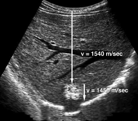
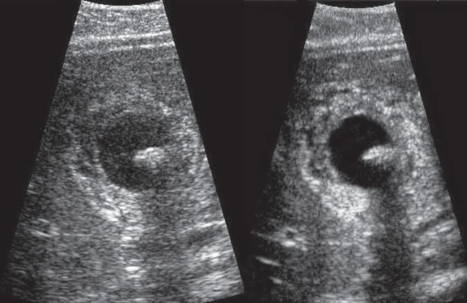
FIG. 1.3 Propagation Velocity Artifact. When sound passes through a lesion containing fat, echo return is delayed because fat has a propagation velocity of 1450 m/sec, which is less than the liver. Because the ultrasound scanner assumes that sound is being propagated at the average velocity of 1540 m/sec, the delay in echo return is interpreted as indicating a deeper target. Therefore the final image shows a misregistration artifact in which the diaphragm and other structures deep to the fatty lesion are shown in a deeper position than expected (simulated image).
which the velocity is determined by Young modulus, a measure of tissue stiffness or elasticity.
Fig. 1.2 shows typical longitudinal propagation velocities for a variety of materials. In the body the propagation velocity of sound is assumed to be 1540 meters per second (m/sec). This value is the average of measurements obtained from normal soft tissue.2,3 Although this value represents most soft tissues, such tissues as aerated lung and fat have propagation velocities significantly less than 1540 m/sec, whereas tissues such as bone have greater velocities. Because a few normal tissues have propagation values significantly different from the average value assumed by the ultrasound scanner, the display of such tissues may be subject to measurement errors or artifacts (Fig. 1.3). The propagation velocity of sound (c) is related to frequency and wavelength by the following simple equation: c
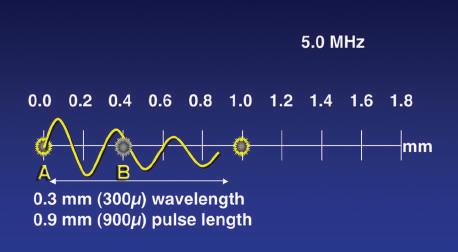
Thus a frequency of 5 MHz can be shown to have a wavelength of 0.308 mm in tissue: λ = c/f = 1540 m/sec × 5,000,000 sec 1 = 0.000308 m = 0.308 mm. Wavelength is an important determinant of spatial resolution in ultrasound imaging, and selection of transducer frequency for a given application is a key user decision.
Distance Measurement
Propagation velocity is a particularly important value in clinical ultrasound and is critical in determining the distance of a reflecting interface from the transducer. Much of the information used to generate an ultrasound scan is based on the precise measurement of time and employs the principles of echo-ranging (Fig. 1.4). If an ultrasound pulse is transmitted into the body and the time until an echo returns is measured, it is simple to calculate the depth of the interface that generated the echo, provided the
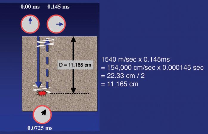
propagation velocity of sound for the tissue is known. For example, if the time from the transmission of a pulse until the return of an echo is 0.000145 seconds and the velocity of sound is 1540 m/ sec, the distance that the sound has traveled must be 22.33 cm (1540 m/sec × 100 cm/m × 0.000145 sec = 22.33 cm). Because the time measured includes the time for sound to travel to the interface and then return along the same path to the transducer, the distance from the transducer to the reflecting interface is 22.33 cm/2 = 11.165 cm. By rapidly repeating this process, a two-dimensional (2-D) map of reflecting interfaces is created to form the ultrasound image. The accuracy of this measurement is therefore highly influenced by how closely the presumed velocity of sound corresponds to the true velocity in the tissue being observed (see Figs. 1.2 and 1.3), as well as by the important assumption that the sound pulse travels in a straight path to and from the reflecting interface.
Acoustic Impedance
Current diagnostic ultrasound scanners rely on the detection and display of reflected sound or echoes. Imaging based on transmission of ultrasound is also possible, but this is not used clinically at present. To produce an echo, a reflecting interface must be present. Sound passing through a totally homogeneous medium encounters no interfaces to reflect sound, and the medium appears anechoic or cystic. The junction of tissues or materials with different physical properties produces an acoustic interface. These interfaces are responsible for the reflection of variable amounts of the incident sound energy. Thus when ultrasound passes from one tissue to another or encounters a vessel wall or circulating blood cells, some of the incident sound
ms
FIG. 1.4 Ultrasound Ranging. The information used to position an echo for display is based on the precise measurement of time. Here the time for an echo to travel from the transducer to the target and return to the transducer is 0.145 ms (0.000145 seconds). Multiplying the velocity of sound in tissue (1540 m/sec) by the time shows that the sound returning from the target has traveled 22.33 cm. Therefore the target lies half this distance, or 11.165 cm, from the transducer. By rapidly repeating this process, a two-dimensional map of reflecting interfaces is created to form the ultrasound image.
energy is reflected. The amount of reflection or backscatter is determined by the difference in the acoustic impedances of the materials forming the interface.
Acoustic impedance (Z) is determined by product of the density (ρ) of the medium propagating the sound and the propagation velocity (c) of sound in that medium (Z = ρc). Interfaces with large acoustic impedance differences, such as interfaces of tissue with air or bone, reflect almost all the incident energy. Interfaces composed of substances with smaller differences in acoustic impedance, such as a muscle and fat interface, reflect only part of the incident energy, permitting the remainder to continue onward. As with propagation velocity, acoustic impedance is determined by the properties of the tissues involved and is independent of frequency.
Reflection
The way ultrasound is reflected when it strikes an acoustic interface is determined by the size and surface features of the interface (Fig. 1.5). If large and relatively smooth, the interface reflects sound much as a mirror reflects light. Such interfaces are called specular reflectors because they behave as “mirrors for sound.” The amount of energy reflected by an acoustic interface can be expressed as a fraction of the incident energy; this is termed the reflection coefficient (R). If a specular reflector is perpendicular to the incident sound beam, the amount of energy reflected is determined by the following relationship:
RZZZZ =−+()() 21 2 21 2 where Z1 and Z2 are the acoustic impedances of the media forming the interface.
Because ultrasound scanners only detect reflections that return to the transducer, display of specular interfaces is highly dependent
Examples of Specular Reflectors
Diaphragm
Vessel wall
Wall of urine-filled bladder
Endometrial stripe
on the angle of insonation (exposure to ultrasound waves). Specular reflectors will return echoes to the transducer only if the sound beam is perpendicular to the interface. If the interface is not at a near 90-degree angle to the sound beam, it will be reflected away from the transducer, and the echo will not be detected (see Fig. 1.5A).
Most echoes in the body do not arise from specular reflectors but rather from much smaller interfaces within solid organs. In this case the acoustic interfaces involve structures with individual dimensions much smaller than the wavelength of the incident sound. The echoes from these interfaces are scattered in all directions. Such reflectors are called diffuse reflectors and account for the echoes that form the characteristic echo patterns seen in solid organs and tissues (see Fig. 1.5B). The constructive and destructive interference of sound scattered by diffuse reflectors results in the production of ultrasound speckle, a feature of tissue texture of sonograms of solid organs (Fig. 1.6). For some diagnostic applications, the nature of the reflecting structures creates important conflicts. For example, most vessel walls behave as specular reflectors that require insonation at a 90-degree angle for best imaging, whereas Doppler imaging requires an angle of less than 90 degrees between the sound beam and the vessel.


FIG. 1.5 Specular and Diffuse Reflectors. (A) Specular reflector. The diaphragm is a large and relatively smooth surface that reflects sound like a mirror reflects light. Thus sound striking the diaphragm at nearly a 90-degree angle is reflected directly back to the transducer, resulting in a strong echo. Sound striking the diaphragm obliquely is reflected away from the transducer, and an echo is not displayed (yellow arrow). (B) Diffuse reflector. In contrast to the diaphragm, the liver parenchyma consists of acoustic interfaces that are small compared to the wavelength of sound used for imaging. These interfaces scatter sound in all directions, and only a portion of the energy returns to the transducer to produce the image.

FIG. 1.6 Ultrasound Speckle. Close inspection of an ultrasound image of the breast containing a small cyst reveals it to be composed of numerous areas of varying intensity (speckle). Speckle results from the constructive (red) and destructive (green) interaction of the acoustic fields (yellow rings) generated by the scattering of ultrasound from small tissue reflectors. This interference pattern gives ultrasound images their characteristic grainy appearance and may reduce contrast. Ultrasound speckle is the basis of the texture displayed in ultrasound images of solid tissues.
Refraction
When sound passes from a tissue with one acoustic propagation velocity to a tissue with a higher or lower sound velocity, there is a change in the direction of the sound wave. This change in direction of propagation is called refraction and is governed by Snell law:
sinsinθθ1212 = cc
where θ1 is the angle of incidence of the sound approaching the interface, θ2 is the angle of refraction, and c1 and c2 are the
propagation velocities of sound in the media forming the interface (Fig. 1.7). Refraction is important because it is one cause of misregistration of a structure in an ultrasound image (Fig. 1.8). When an ultrasound scanner detects an echo, it assumes that the source of the echo is along a fixed line of sight from the transducer. If the sound has been refracted, the echo detected may be coming from a different depth or location than the image shown in the display. If this is suspected, increasing the scan angle so that it is perpendicular to the interface minimizes the artifact.
Attenuation
As the acoustic energy moves through a uniform medium, work is performed and energy is ultimately transferred to the transmitting medium as heat. The capacity to perform work is determined by the quantity of acoustic energy produced. Acoustic power, expressed in watts (W) or milliwatts (mW), describes the amount of acoustic energy produced in a unit of time. Although measurement of power provides an indication of the energy as it relates to time, it does not take into account the spatial distribution of the energy. Intensity (I) is used to describe the spatial distribution of power and is calculated by dividing the power by the area over which the power is distributed, as follows:
IW/cmPowerWAreacm ()()() 2 2 =
The attenuation of sound energy as it passes through tissue is of great clinical importance because it influences the depth in tissue from which useful information can be obtained. This in turn affects transducer selection and a number of operatorcontrolled instrument settings, including time (or depth) gain compensation, power output attenuation, and system gain levels. Attenuation is measured in relative rather than absolute units. The decibel (dB) notation is generally used to compare different levels of ultrasound power or intensity. This value is 10 times the log10 of the ratio of the power or intensity values being
Tissue A
c1 = 1540 m/sec
Tissue B
c2 = 1450 m/sec
FIG. 1.7 Refraction. When sound passes from tissue A with propagation velocity (c1) to tissue B with a different propagation velocity (c2), there is a change in the direction of the sound wave because of refraction. The degree of change is related to the ratio of the propagating velocities of the media forming the interface (sinθ1/sinθ2 = c1/c2). θ1 = 20° θ2 = 18.8° 188
compared. For example, if the intensity measured at one point in tissues is 10 mW/cm2 and at a deeper point is 0.01 mW/cm2, the difference in intensity is as follows:
()()()() log.()log.()log ()( 1000110100001101000 10 10 10 10 = =− =−3330) =− dB
As it passes through tissue, sound loses energy, and the pressure waves decrease in amplitude as they travel farther from their source. Contributing to the attenuation of sound are the transfer of energy to tissue, resulting in heating (absorption), and the removal of energy by reflection and scattering. Attenuation is therefore the result of the combined effects of absorption, scattering, and reflection. Attenuation depends on the insonating frequency as well as the nature of the attenuating medium. High frequencies are attenuated more rapidly than lower frequencies, and transducer frequency is a major determinant of the useful depth from which information can be obtained with ultrasound. Attenuation determines the efficiency with which ultrasound

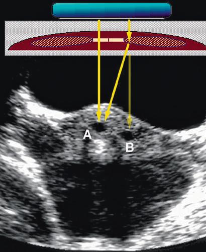
FIG. 1.8 Refraction Artifact. (A) and (B) Production of an artifact by refraction of sound in a transverse scan of the mid abdomen. The direct sound path properly depicts the location of the object. (B) A “ghost image” (red) produced by refraction at the edge of the rectus abdominis muscle. The transmitted and reflected sound travels along the path of the black arrows. The scanner assumes the returning signal is from a straight line (red arrow) and displays the structure at the incorrect location. (C) Axial transabdominal image of the uterus showing a small gestational sac (A) and what appears to be a second sac (B) due to refraction artifact.
FIG. 1.9 Attenuation. As sound passes through tissue, it loses energy through the transfer of energy to tissue by heating, reflection, and scattering. Attenuation is determined by the insonating frequency and the nature of the attenuating medium. Attenuation values for normal tissues show considerable variation. Attenuation also increases in proportion to insonating frequency, resulting in less penetration at higher frequencies.
penetrates a specific tissue and varies considerably in normal tissues (Fig. 1.9).
INSTRUMENTATION
Ultrasound scanners are complex and sophisticated imaging devices, but all consist of the following basic components to perform key functions:
• Transmitter or pulser to energize the transducer
• Ultrasound transducer
• Receiver and processor to detect and amplify the backscattered energy and manipulate the reflected signals for display
• Display that presents the ultrasound image or data in a form suitable for analysis and interpretation
• Method to record or store the ultrasound image
Transmitter
Most clinical applications use pulsed ultrasound, in which brief bursts of acoustic energy are transmitted into the body. The source of these pulses, the ultrasound transducer, is energized by application of precisely timed, high-amplitude voltage. The maximum voltage that may be applied to the transducer is limited by federal regulations that restrict the acoustic output of diagnostic scanners. Most scanners provide a control that permits attenuation of the output voltage. Because the use of maximum output results in higher exposure of the patient to ultrasound energy, prudent use dictates use of the output attenuation controls to reduce power levels to the lowest levels consistent with the diagnostic problem.4
The transmitter also controls the rate of pulses emitted by the transducer, or the pulse repetition frequency (PRF). The
PRF determines the time interval between ultrasound pulses and is important in determining the depth from which unambiguous data can be obtained both in imaging and Doppler modes. The ultrasound pulses must be spaced with enough time between the pulses to permit the sound to travel to the depth of interest and return before the next pulse is sent. For imaging, PRFs from 1 to 10 kHz are used, resulting in an interval of 0.1 to 1 ms between pulses. Thus a PRF of 5 kHz permits an echo to travel and return from a depth of 15.4 cm before the next pulse is sent.
Transducer
A transducer is any device that converts one form of energy to another. In ultrasound the transducer converts electric energy to mechanical energy, and vice versa. In diagnostic ultrasound systems the transducer serves two functions: (1) converting the electric energy provided by the transmitter to the acoustic pulses directed into the patient and (2) serving as the receiver of reflected echoes, converting weak pressure changes into electric signals for processing.
Ultrasound transducers use piezoelectricity, a principle discovered by Pierre and Jacques Curie in 1880.5 Piezoelectric materials have the unique ability to respond to the action of an electric field by changing shape. They also have the property of generating electric potentials when compressed. Changing the polarity of a voltage applied to the transducer changes the thickness of the transducer, which expands and contracts as the polarity changes. This results in the generation of mechanical pressure waves that can be transmitted into the body. The piezoelectric effect also results in the generation of small potentials across the transducer when the transducer is struck by returning echoes. Positive pressures cause a small polarity to develop across the transducer; negative pressure during the rarefaction portion of the acoustic wave produces the opposite polarity across the transducer. These tiny polarity changes and the associated voltages are the source of all the information processed to generate an ultrasound image or Doppler display.
When stimulated by the application of a voltage difference across its thickness, the transducer vibrates. The frequency of vibration is determined by the transducer material. When the transducer is electrically stimulated, a range or band of frequencies results. The preferential frequency produced by a transducer is determined by the propagation speed of the transducer material and its thickness. In the pulsed wave operating modes used for most clinical ultrasound applications, the ultrasound pulses contain additional frequencies that are both higher and lower than the preferential frequency. The range of frequencies produced by a given transducer is termed its bandwidth. Generally, the shorter the pulse of ultrasound produced by the transducer, the greater is the bandwidth.
Most modern digital ultrasound systems employ broadbandwidth technology. Ultrasound bandwidth refers to the range of frequencies produced and detected by the ultrasound system. This is important because each tissue in the body has a characteristic response to ultrasound of a given frequency, and different tissues respond differently to different frequencies. The range of frequencies arising from a tissue exposed to ultrasound is referred to as the frequency spectrum bandwidth of the tissue, or tissue
signature. Broad-bandwidth technology provides a means to capture the frequency spectrum of insonated tissues, preserving acoustic information and tissue signature. Broad-bandwidth beam formers reduce speckle artifact by a process of frequency compounding. This is possible because speckle patterns at different frequencies are independent of one another, and combining data from multiple frequency bands (i.e., compounding) results in a reduction of speckle in the final image, leading to improved contrast resolution.
The length of an ultrasound pulse is determined by the number of alternating voltage changes applied to the transducer. For continuous wave (CW) ultrasound devices, a constant alternating current is applied to the transducer, and the alternating polarity produces a continuous ultrasound wave. For imaging, a single, brief voltage change is applied to the transducer, causing it to vibrate at its preferential frequency. Because the transducer continues to vibrate or “ring” for a short time after it is stimulated by the voltage change, the ultrasound pulse will be several cycles long. The number of cycles of sound in each pulse determines the pulse length. For imaging, short pulse lengths are desirable because longer pulses result in poorer axial resolution. To reduce the pulse length, damping materials are used in the construction of the transducer. In clinical imaging applications, very short pulses are applied to the transducer, and the transducers have highly efficient damping. This results in very short pulses of ultrasound, generally consisting of only two or three cycles of sound.
The ultrasound pulse generated by a transducer must be propagated in tissue to provide clinical information. Special transducer coatings and ultrasound coupling gels are necessary to allow efficient transfer of energy from the transducer to the body. Once in the body, the ultrasound pulses are propagated, reflected, refracted, and absorbed, in accordance with the basic acoustic principles summarized earlier.
The ultrasound pulses produced by the transducer result in a series of wavefronts that form a three-dimensional (3-D) beam of ultrasound. The features of this beam are influenced by
constructive and destructive interference of the pressure waves, the curvature of the transducer, and acoustic lenses used to shape the beam. Interference of pressure waves results in an area near the transducer where the pressure amplitude varies greatly. This region is termed the near field, or Fresnel zone. Farther from the transducer, at a distance determined by the radius of the transducer and the frequency, the sound field begins to diverge, and the pressure amplitude decreases at a steady rate with increasing distance from the transducer. This region is called the far field, or Fraunhofer zone. In modern multielement transducer arrays, precise timing of the firing of elements allows correction of this divergence of the ultrasound beam and focusing at selected depths. Only reflections of pulses that return to the transducer are capable of stimulating the transducer with small pressure changes, which are converted into the voltage changes that are detected, amplified, and processed to build an image based on the echo information.
Receiver
When returning echoes strike the transducer face, minute voltages are produced across the piezoelectric elements. The receiver detects and amplifies these weak signals. The receiver also provides a means for compensating for the differences in echo strength, which result from attenuation by different tissue thickness by control of time gain compensation (TGC) or depth gain compensation (DGC).
Sound is attenuated as it passes into the body, and additional energy is removed as echoes return through tissue to the transducer. The attenuation of sound is proportional to the frequency and is constant for specific tissues. Because echoes returning from deeper tissues are weaker than those returning from more superficial structures, they must be amplified more by the receiver to produce a uniform tissue echo appearance (Fig. 1.10). This adjustment is accomplished by TGC controls that permit the user to selectively amplify the signals from deeper structures or to suppress the signals from superficial tissues, compensating for tissue attenuation. Although many newer machines provide

FIG. 1.10 Time Gain Compensation (TGC). Without TGC, tissue attenuation causes gradual loss of display of deeper tissues (A). In this example, tissue attenuation of 1 dB/cm/MHz is simulated for a transducer of 10 MHz. At a depth of 2 cm, the intensity is 20 dB (1% of initial value). By applying increasing amplification or gain to the backscattered signal to compensate for this attenuation, a uniform intensity is restored to the tissue at all depths (B).
for some means of automatic TGC, the manual adjustment of this control is one of the most important user controls and may have a profound effect on the quality of the ultrasound image provided for interpretation.
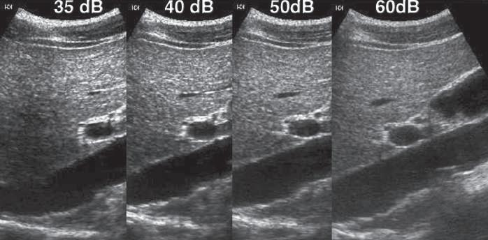
Another important function of the receiver is the compression of the wide range of amplitudes returning to the transducer into a range that can be displayed to the user. The ratio of the highest to the lowest amplitudes that can be displayed may be expressed in decibels and is referred to as the dynamic range. In a typical clinical application, the range of reflected signals may vary by a factor of as much as 1 : 1012, resulting in a dynamic range of up to 120 dB. Although the amplifiers used in ultrasound machines are capable of handling this range of voltages, gray-scale displays are limited to display a signal intensity range of only 35 to 40 dB. Compression and remapping of the data are required to adapt the dynamic range of the backscattered signal intensity to the dynamic range of the display (Fig. 1.11). Compression is performed in the receiver by selective amplification of weaker signals. Additional manual postprocessing controls permit the user to map selectively the returning signal to the display. These controls affect the brightness of different echo levels in the image and therefore determine the image contrast.
Image Display
Ultrasound signals may be displayed in several ways. Over the years, imaging has evolved from simple A-mode (amplitudemode) and bistable display to high-resolution, real-time, grayscale imaging. The earliest A-mode devices displayed the voltage produced across the transducer by the backscattered echo as a vertical deflection on the face of an oscilloscope. The horizontal time sweep of the oscilloscope was calibrated to indicate the distance from the transducer to the reflecting surface. In this form of display, the strength or amplitude of the reflected sound is indicated by the height of the vertical deflection displayed on the oscilloscope. With A-mode ultrasound, only the position and strength of a reflecting structure are recorded.
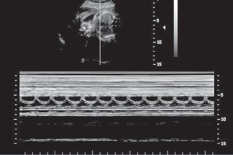
Another simple form of imaging, M-mode (motion-mode) ultrasound, displays echo amplitude and shows the position of
changes of echo amplitude and position with time. Display of changes in echo position is useful in the evaluation of rapidly moving structures such as cardiac valves and chamber walls. Here, the three major moving structures in the upper gray-scale image of the fetus are recorded in the corresponding M-mode image and include the near ventricular wall (A), the interventricular septum (B), and the far ventricular wall (C). The baseline is a time scale that permits the calculation of heart rate from the M-mode data.
moving reflectors (Fig. 1.12). M-mode imaging uses the brightness of the display to indicate the intensity of the reflected signal. The time base of the display can be adjusted to allow for varying degrees of temporal resolution, as dictated by clinical application. M-mode ultrasound is interpreted by assessing motion patterns of specific reflectors and determining anatomic relationships from characteristic patterns of motion. Currently, the major application of M-mode display is evaluation of embryonic and fetal heart rates, as well as in echocardiography, the rapid motion of cardiac valves and of cardiac chamber and vessel walls. M-mode imaging may play a future role in measurement of subtle changes in vessel wall elasticity accompanying atherogenesis.
The mainstay of imaging with ultrasound is provided by real-time, gray-scale, B-mode display, in which variations in display intensity or brightness are used to indicate reflected signals
FIG. 1.11 Dynamic Range. The ultrasound receiver must compress the wide range of amplitudes returning to the transducer into a range that can be displayed to the user. Here, compression and remapping of the data to display dynamic ranges of 35, 40, 50, and 60 dB are shown. The widest dynamic range shown (60 dB) permits the best differentiation of subtle differences in echo intensity and is preferred for most imaging applications. The narrower ranges increase conspicuity of larger echo differences.
FIG. 1.12 M-Mode Display. M-mode ultrasound displays
of differing amplitude. To generate a 2-D image, multiple ultrasound pulses are sent down a series of successive scan lines (Fig. 1.13), building a 2-D representation of echoes arising from the object being scanned. When an ultrasound image is displayed on a black background, signals of greatest intensity appear as white; absence of signal is shown as black; and signals of intermediate intensity appear as shades of gray. If the ultrasound beam is moved with respect to the object being examined and the position of the reflected signal is stored, the brightest portions of the resulting 2-D image indicate structures reflecting more of the transmitted sound energy back to the transducer.
In most modern instruments, digital memory is used to store values that correspond to the echo intensities originating from corresponding positions in the patient. At least 28, or 256, shades of gray are possible for each pixel, in accord with the amplitude of the echo being represented. The image stored in memory in this manner can then be sent to a monitor for display.
Because B-mode display relates the strength of a backscattered signal to a brightness level on the display device, it is important that the operator understand how the amplitude information in the ultrasound signal is translated into a brightness scale in the image display. Each ultrasound manufacturer offers several options
for the way the dynamic range of the target is compressed for display, as well as the transfer function that assigns a given signal amplitude to a shade of gray. Although these technical details vary among machines, the way the operator uses them may greatly affect the clinical value of the final image. In general, it is desirable to display as wide a dynamic range as possible, to identify subtle differences in tissue echogenicity (see Fig. 1.11).
Real-time ultrasound produces the impression of motion by generating a series of individual 2-D images at rates of 15 to 60 frames per second. Real-time, 2-D, B-mode ultrasound is the major method for ultrasound imaging throughout the body and is the most common form of B-mode display. Real-time ultrasound permits assessment of both anatomy and motion. When images are acquired and displayed at rates of several times per second, the effect is dynamic, and because the image reflects the state and motion of the organ at the time it is examined, the information is regarded as being shown in real time. In cardiac applications the terms 2-D echocardiography and 2-D echo are used to describe real-time, B-mode imaging; in most other applications the term real-time ultrasound is used.
Transducers used for real-time imaging may be classified by the method used to steer the beam in rapidly generating each
FIG. 1.13 B-Mode Imaging. A two-dimensional (2-D), real-time image is built by ultrasound pulses sent down a series of successive scan lines. Each scan line adds to the image, building a 2-D representation of echoes from the object being scanned. In real-time imaging, an entire image is created 15 to 60 times per second.
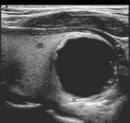

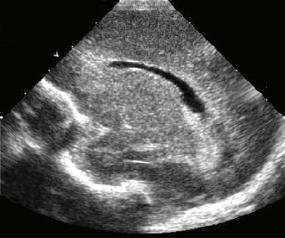
FIG. 1.14 Beam Steering. (A) Linear array. In a linear array transducer, individual elements or groups of elements are fired in sequence. This generates a series of parallel ultrasound beams, each perpendicular to the transducer face. As these beams move across the transducer face, they generate the lines of sight that combine to form the final image. Depending on the number of transducer elements and the sequence in which they are fired, focusing at selected depths from the surface can be achieved Small high-frequency linear arrays are well-suited for small parts scanning. (B) Curved array. A variant of the linear array, the curved array uses tranducer elements arranged in an arc, producing a pie-shaped image. These transducers are well-suited for abdominal, pelvic, and fetal examinations. (C) Phased array. A phased array transducer produces a sector field of view by firing multiple transducer elements in precise sequence to generate interference of acoustic wavefronts that steer the beam. The ultrasound beam that results generates a series of lines of sight at varying angles from one side of the transducer to the other, producing a sector image format. These transducers require a small contact area compared to most linear and curved arrays and are useful for scanning in areas where access is limited.
individual image, keeping in mind that as many as 30 to 60 complete images must be generated per second for real-time applications. Beam steering may be done through mechanical rotation or oscillation of the transducer or by electronic means (Fig. 1.14). Electronic beam steering is used in linear array and phased array transducers and permits a variety of image display formats. Most electronically steered transducers currently in use also provide electronic focusing that is adjustable for depth. Mechanical beam steering may use single-element transducers with a fixed focus or may use annular arrays of elements with electronically controlled focusing. For real-time imaging, transducers using mechanical or electronic beam steering generate displays in a rectangular or pie-shaped format. For obstetric, small parts, and peripheral vascular examinations, linear array transducers with a rectangular image format are often used. The rectangular image display has the advantage of a larger field of view near the surface but requires a large surface area for transducer contact. Sector scanners with either mechanical or electronic steering require only a small surface area for contact and are better suited for examinations in which access is limited.
Mechanical Sector Scanners
Early ultrasound scanners used transducers consisting of a single piezoelectric element. To generate real-time images with these transducers, mechanical devices were required to move the
transducer in a linear or circular motion. Mechanical sector scanners using one or more single-element transducers do not allow variable focusing. This problem is overcome by using annular array transducers. Although important in the early days of realtime imaging, mechanical sector scanners with fixed-focus, single-element transducers are not presently in common use.
Arrays
Current technology uses a transducer composed of multiple elements, usually produced by precise slicing of a piece of piezoelectric material into numerous small units, each with its own electrodes. Such transducer arrays may be formed in a variety of configurations. Typically, these are linear, curved, phased, or annular arrays. High-density 2-D arrays have also been developed. By precise timing of the firing of combinations of elements in these arrays, interference of the wavefronts generated by the individual elements can be exploited to change the direction of the ultrasound beam, and this can be used to provide a steerable beam for the generation of real-time images in a linear or sector format.
Linear Arrays
Linear array transducers are used for small parts, vascular, and obstetric applications because the rectangular image format produced by these transducers is well suited for these applications.
In these transducers, individual elements are arranged in a linear fashion. By firing the transducer elements in sequence, either individually or in groups, a series of parallel pulses is generated, each forming a line of sight perpendicular to the transducer face. These individual lines of sight combine to form the image field of view (see Fig. 1.14A). Depending on the number of transducer elements and the sequence in which they are fired, focusing at selected depths from the surface can be achieved.
Curved Arrays
Linear arrays that have been shaped into convex curves produce an image that combines a relatively large surface field of view with a sector display format (see Fig. 1.14B). Curved array transducers are used for a variety of applications, the larger versions serving for general abdominal, obstetric, and transabdominal pelvic scanning. Small, high-frequency, curved array scanners are often used in transvaginal and transrectal probes and for pediatric imaging.
Phased Arrays
In contrast to mechanical sector scanners, phased array scanners have no moving parts. A sector field of view is produced by multiple transducer elements fired in precise sequence under electronic control. By controlling the time and sequence at which the individual transducer elements are fired, the resulting ultrasound wave can be steered in different directions as well as focused at different depths (see Fig. 1.14C). By rapidly steering the beam to generate a series of lines of sight at varying angles from one side of the transducer to the other, a sector image format is produced. This allows the fabrication of transducers of relatively small size but with large fields of view at depth. These transducers are particularly useful for neonatal head ultrasound, as well as for intercostal scanning, to evaluate the heart, liver, or spleen, and for examinations in other areas where access is limited.
Two-Dimensional Arrays
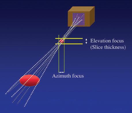
Transducer arrays can be formed either by slicing a rectangular piece of transducer material perpendicular to its long axis to produce a number of small rectangular elements or by creating a series of concentric elements nested within one another in a circular piece of piezoelectric material to produce an annular array. The use of multiple elements permits precise focusing. A particular advantage of 2-D array construction is that the beam can be focused in both the elevation plane and the lateral plane, and a uniform and highly focused beam can be produced (Fig 1.15). These arrays improve spatial resolution and contrast, reduce clutter, and are well suited for the collection of data from volumes of tissue for use in 3-D processing and display. Unlike linear 2-D arrays, in which delays in the firing of the individual elements may be used to steer the beam, annular arrays do not permit beam steering and, to be used for real-time imaging, must be steered mechanically.
Transducer Selection
Practical considerations in the selection of the optimal transducer for a given application include not only the requirements for
1.15 Two-Dimensional Array. High-density, two-dimensional (2-D) arrays consist of a 2-D matrix of transducer elements, permitting acquisition of data from a volume rather than a single plane of tissue. Precise electronic control of individual elements permits adjustable focusing on both azimuth and elevation planes.
spatial resolution, but also the distance of the target object from the transducer because penetration of ultrasound diminishes as frequency increases. In general, the highest ultrasound frequency permitting penetration to the depth of interest should be selected. For superficial vessels and organs, such as the thyroid, breast, or testicle, lying within 1 to 3 cm of the surface, imaging frequencies of 7.5 to 15 MHz are typically used. These high frequencies are also ideal for intraoperative applications. If the region to be scanned is very superficial, such that the probe does not allow for focusing at the area of interest, a standoff pad can be utilized. For evaluation of deeper structures in the abdomen or pelvis more than 12 to 15 cm from the surface, frequencies as low as 2.25 to 3.5 MHz may be required. When maximal resolution is needed, a high-frequency transducer with excellent lateral and elevation resolution at the depth of interest is required.
IMAGE DISPLAY AND STORAGE
With real-time ultrasound, user feedback is immediate and is provided by video display. The brightness and contrast of the image on this display are determined by the ambient lighting in the examination room, the brightness and contrast settings of the video monitor, the system gain setting, and the TGC adjustment. The factor most affecting image quality in many ultrasound departments is probably improper adjustment of the video display, with a lack of appreciation of the relationship between the video display settings and the appearance of hard copy or images viewed on a workstation. Because of the importance of the real-time video display in providing feedback to the user, it is essential that the display and the lighting conditions under which it is viewed are standardized and matched to the display used for interpretation. Interpretation of images and archival storage of images may be in the form of transparencies printed on film by optical or laser cameras and printers, videotape, or digital picture
FIG.
FIG. 1.16 Tissue Harmonics. As sound is propagated through tissue, the high-pressure component of the wave travels more rapidly than the rarefactional component, producing distortion of the wave and generating higher-frequency components (harmonics). (A) The acoustic field of the primary frequency is represented in blue. (B) The second harmonic (twice the primary frequency) is represented in red. (C) Using a broad-bandwidth transducer, the receiver can be tuned to generate an image from the harmonic frequency rather than the primary frequency. As a result, near field clutter is reduced since the harmonic only develops at depth in the tissue and the beam profile is improved, leading to better spatial resolution.
archiving and communications system (PACS). Increasingly, digital storage is being used for archiving of ultrasound images.
SPECIAL IMAGING MODES
Tissue Harmonic Imaging
Variation of the propagation velocity of sound in fat and other tissues near the transducer results in a phase aberration that distorts the ultrasound field, producing noise and clutter in the ultrasound image. Tissue harmonic imaging provides an approach for reducing the effects of phase aberrations.6 Nonlinear propagation of ultrasound through tissue is associated with the more rapid propagation of the high-pressure component of the ultrasound pressure wave than its negative (rarefactional) component. This results in increasing distortion of the acoustic pulse as it travels within the tissue and causes the generation of multiples, or harmonics, of the transmitted frequency (Fig. 1.16).
Tissue harmonic imaging takes advantage of the generation, at depth, of these harmonics. Because the generation of harmonics requires interaction of the transmitted field with the propagating tissue, harmonic generation is not present near the transducer/ skin interface, and it only becomes important some distance from the transducer. In most cases the near and far fields of the image are affected less by harmonics than by intermediate locations. Using broad-bandwidth transducers and signal filtration or coded pulses, the harmonic signals reflected from tissue
interfaces can be selectively displayed. Because most imaging artifacts are caused by the interaction of the ultrasound beam with superficial structures or by aberrations at the edges of the beam profile, these artifacts are eliminated using harmonic imaging because the artifact-producing signals do not consist of sufficient energy to generate harmonic frequencies and therefore are filtered out during image formation. Images generated using tissue harmonics often exhibit reduced noise and clutter (Fig. 1.17). Because harmonic beams are narrower than the originally transmitted beams, spatial resolution is improved and side lobes are reduced.
Spatial Compounding
An important source of image degradation and loss of contrast is ultrasound speckle. Speckle results from the constructive and destructive interaction of the acoustic fields generated by the scattering of ultrasound from small tissue reflectors. This interference pattern gives ultrasound images their characteristic grainy appearance (see Fig. 1.6), reducing contrast (Fig. 1.18) and making the identification of subtle features more difficult. By summing images from different scanning angles through spatial compounding (Fig. 1.19), significant improvement in the contrast-to-noise ratio can be achieved (Fig. 1.20). This is because speckle is random, and the generation of an image by compounding will reduce speckle noise because only the signal is reinforced. In addition, spatial compounding may reduce artifacts that result when an ultrasound beam strikes a specular reflector at an angle
FIG. 1.17 Tissue Harmonic Imaging. (A)
Conventional image and (B) tissue harmonic image of gallbladder of patient with acute cholecystitis. Note the reduction of noise and clutter in the tissue harmonic image. Because harmonic beams do not interact with superficial structures and are narrower than the originally transmitted beam, spatial resolution is improved and clutter and side lobes are reduced. (With permission from Merritt CR. Technology update. Radiol Clin North Am. 2001;39:385-397.7)
FIG. 1.18 Effect of Speckle on Contrast. (A)
Speckle noise partially obscures the simulated lesion. (B) The speckle has been reduced, increasing contrast resolution between the lesion and the background. (With permission from Merritt CR. Technology update. Radiol Clin North Am. 2001;39:385-397.7)
FIG. 1.19 Spatial Compounding. (A) Conventional imaging is limited to a fixed angle of incidence of ultrasound scan lines to tissue interfaces, resulting in poor definition of specular reflectors that are not perpendicular to the beam. (B) Spatial compounding combines images obtained by insonating the target from multiple angles. In addition to improving detection of interfaces, compounding reduces speckle noise because only the signal is reinforced; speckle is random and not reinforced. This improves contrast.


greater or less than 90 degrees. In conventional real-time imaging, each scan line used to generate the image strikes the target at a constant, fixed angle. As a result, strong reflectors that are not perpendicular to the ultrasound beam scatter sound in directions that prevent their clear detection and display. This in turn results in poor margin definition and less distinct boundaries for cysts and other masses. Compounding has been found to reduce these artifacts. Limitations of compounding are diminished visibility of shadowing and enhancement; however, these are offset by the ability to evaluate lesions, both with and without compounding, preserving shadowing and enhancement when these features are important to diagnosis.7
Three-Dimensional Ultrasound
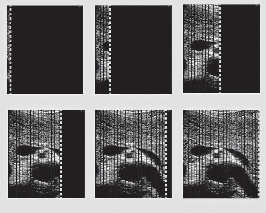
Dedicated 3-D scanners used for fetal (Fig. 1.21), gynecologic, and cardiac scanning may employ hardware-based image registration, high-density 2-D arrays, or software registration of scan planes as a tissue volume is acquired. 3-D imaging permits volume
data to be viewed in multiple imaging planes and allows accurate measurement of lesion volume.
Ultrasound Elastography
Palpation is an effective method for detection of tissue abnormality based on detection of changes in tissue stiffness or elasticity and may provide the earliest indication of disease, even when conventional imaging studies are normal. Ultrasound elastography provides a noninvasive method for evaluation of tissue stiffness.8
Tissue contrast in conventional ultrasound imaging is based on the bulk modulus determined by the molecular composition of tissue, whereas elastography reflects shear properties that are determined by a higher level of tissue organization, the strain modulus. This higher level of tissue organization is most likely to be altered by disease. The dynamic range of the strain modulus is several orders of magnitude greater than the bulk modulus, permitting contrast resolution far exceeding conventional ultrasound imaging.9 Elastography therefore offers the potential for a
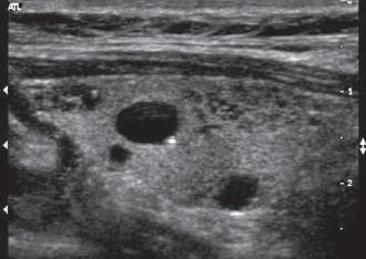
FIG. 1.20 Spatial Compounding. (A) Conventional image and (B) compound image of the thyroid. Note the reduced speckle as well as better definition of regions (arrows) such as superficial tissue as well as small cysts and calcifications.
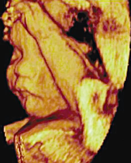
FIG. 1.21 Three-Dimensional Ultrasound Image, 24-Week Fetus. Three-dimensional ultrasound permits collection and review of data obtained from a volume of tissue in multiple imaging planes, as well as a rendering of surface features.
high degree of both sensitivity and specificity in differentiating normal and abnormal tissues.8,10,11
Tissue stiffness or elasticity is expressed by Young modulus the ratio of compression pressure (stress) and the resulting deformation (strain)
E =σε
where E is Young modulus expressed in Pa (pascals), σ is the stress, expressed in Newtons, and ε is displacement expressed in m2
Ultrasound-based elastography permits study of the elastic behavior of tissue through two general approaches (Fig. 1.22): strain elastography and shear wave elastography.
Strain Elastography
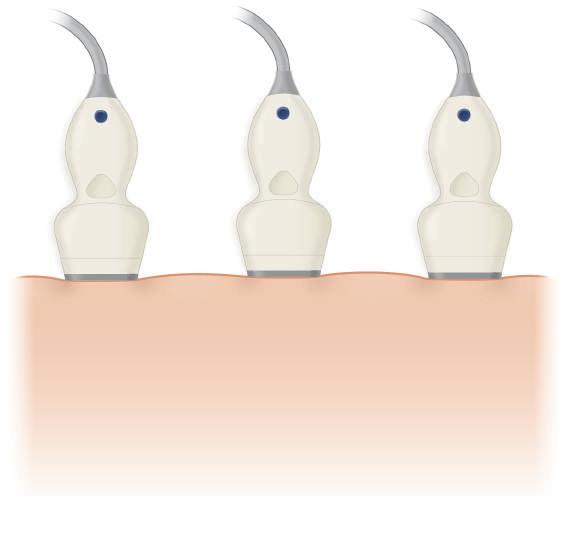
Strain elastography involves measurement of longitudinal tissue displacement before and after compression, usually by manual manipulation of the ultrasound transducer (see Fig. 1.22A). Speckle tracking using radiofrequency backscatter or Doppler is then used to evaluate tissue motion. Strain elastography cannot determine the Young modulus because the compression pressure (stress) cannot be measured directly. Instead, strain ratios are estimated by comparing lesion strain to surrounding normal tissues and displayed in the image in different shades of gray or through color maps (Fig. 1.23). Strain elastography provides an indication of relative stiffness of an area of interest compared to its surroundings.
Key Points of Ultrasound Elastography
Ultrasound imaging is based on tissue bulk modulus, reflecting interactions at the molecular level.
Changes in tissue stiffness based on the tissue shear modulus are important indications of disease.
Ultrasound elastography provides relatative and quantitative assessment of tissue stiffness.
Ultrasound elastography is based on tissue organization (strain modulus).
Strain elastography provides an indication of relative tissue stiffness.
Shear wave elastography provides a quantitative estimate of the tissue stiffness (strain modulus).
Shear Wave Elastography
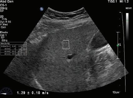
Longitudinal tissue compression results in the generation of transverse shear waves12,13 (see Fig. 1.22B). In shear wave elastography, shear waves are generated by repetitive compression produced by high-intensity pulses from the ultrasound transducer (see Fig. 1.22B). In contrast to longitudinal compressional waves that propagate very quickly in the human body (≈1540 m/sec), shear waves propagate slowly (≈1-50 m/sec). Shear waves are tracked with high frame rate images to determine their velocity. The propagation velocity of shear waves is directly proportional to Young modulus and provides a quantitative estimate of tissue stiffness14,15 (Fig. 1.24).
IMAGE QUALITY
The key determinants of the quality of an ultrasound image are its spatial, contrast, and temporal resolution, as well as freedom from certain artifacts.
Spatial Resolution
The ability to differentiate two closely situated objects as distinct structures is determined by the spatial resolution of the ultrasound device. Spatial resolution must be considered in three planes, with different determinants of resolution for each. Simplest is the resolution along the axis of the ultrasound beam, or axial resolution. With pulsed wave ultrasound, the transducer introduces a series of brief bursts of sound into the body. Each ultrasound pulse typically consists of two or three cycles of sound. The pulse length is the product of the wavelength and the number of cycles in the pulse. Axial resolution, the maximum resolution along the beam axis, is determined by the pulse length (Fig. 1.25). Because ultrasound frequency and wavelength are inversely related, the pulse length decreases as the imaging frequency increases. Because the pulse length determines the maximum resolution along the axis of the ultrasound beam, higher transducer frequencies provide higher image resolution. For example, a transducer operating at 5 MHz produces sound with a wavelength of 0.308 mm. If each pulse consists of three cycles of sound, the pulse length is slightly less than 1 mm, and this becomes the maximum resolution along the beam


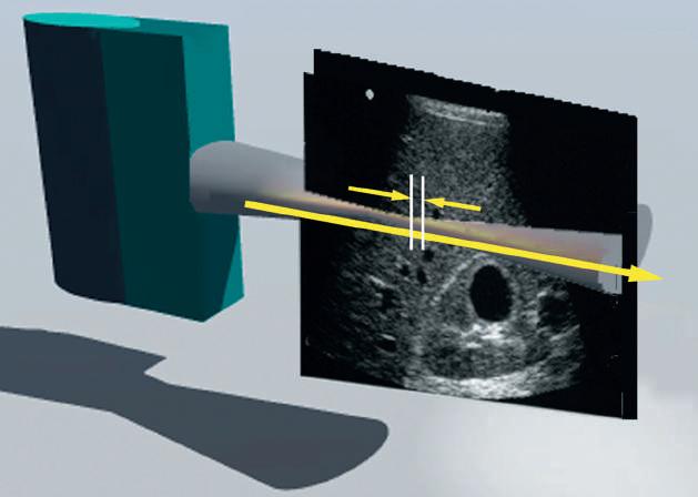
FIG. 1.22 Elastography. (A) Strain elastography (SE), and (B) shear wave elastography (SWE). Strain elastograms are images of tissue stiffness generated by analysis of speckle displacements before and after mechanical compression of tissue. The precompression frame is compared to a frame obtained after compression. In this example, the lesion is compressed much less than the surrounding tissue, indicating relative stiffness. SE is not quantitative and indicates only the relative hardness or softness of lesions compared to their surroundings. In SWE (B) high-intensity compression pulses from the transducer are focused on an area of interest, resulting in the generation of low-frequency shear waves. Speckle displacement resulting from shear (transverse) waves is tracked with multiple imaging frames in order to estimate shear wave velocity. Shear wave velocity is directly related to Young modulus, permitting a quantitative estimate of tissue stiffness.

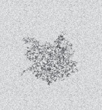
1.23 Strain Elastograms. The upper frames (A) show in vivo images of swine liver containing a lesion produced by the injection of a small volume of absolute ethanol. In the precompression image (left) the lesion located within the circle is invisible. The elastogram (right) clearly delineates the lesion as an area of increased stiffness compared to the surrounding tissue. The lower frames (B) show a gray-scale image (left) and strain elastogram (right) of a mixed solid and cystic thyroid nodule. In the elastogram the color map displays relative stiffness with softer areas appearing as shades of red, orange, and yellow, and stiffer areas as dark blue. The nodule is heterogeneous with the relatively noncompressible cystic portions differentiated from more compressible surrounding tissue. (Courtesy of P. O’Kane, Thomas Jefferson University.)
FIG.
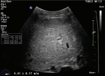
FIG. 1.24 Shear Wave Elastograms of (A) Normal and (B) Cirrhotic Liver. Shear wave velocities measured in liver tissue samples by shear wave elastography indicates a velocity of 1.29 ± 0.10 m/sec in the normal liver compared to a velocity of 4.41 ± 0.17 m/sec in the cirrhotic liver. Increased shear wave velocity is associated with increased tissue stiffness due to hepatic fibrosis. (Courtesy of P. O’Kane, Thomas Jefferson University.)
FIG. 1.25 Axial Resolution. Axial resolution is the resolution along (A) the beam axis and is determined by (B) the pulse length. The pulse length is the product of the wavelength (which decreases with increasing frequency) and the number of waves (usually two to three). Because the pulse length determines axial resolution, higher transducer frequencies provide higher image resolution. In (B) for example, a transducer operating at 5 MHz produces sound with a wavelength of 0.31 mm. If each pulse consists of three cycles of sound, the pulse length is slightly less than 1 mm, and objects A and B, which are 0.5 mm apart, cannot be resolved as separate structures. If the transducer frequency is increased to 15 MHz, the pulse length is less than 0.3 mm, permitting A and B to be identified as separate structures.
A - Normal liver
v = 1.29 ± -.10 m/s
B - Cirrhotic liver
v = 4.41 ± -.17 m/s
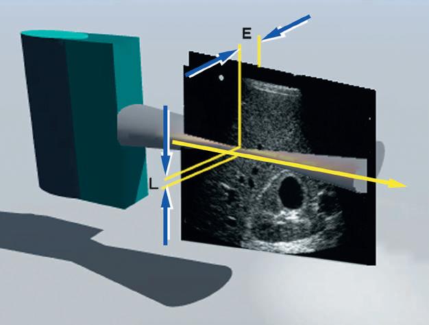
FIG. 1.26 Lateral and Elevation Resolution. Resolution in the planes perpendicular to the beam axis is an important determinant of image quality. Lateral resolution (L) is resolution in the plane perpendicular to the beam and parallel to the transducer and is determined by the width of the ultrasound beam. Lateral resolution is controlled by focusing the beam, usually by electronic phasing to alter the beam width at a selected depth of interest. Azimuth or elevation resolution (E) is determined by the slice thickness in the plane perpendicular to the beam and the transducer. Elevation resolution is controlled by the construction of the transducer. Both lateral resolution and elevation resolution are less than the axial resolution.
axis. If the transducer frequency is increased to 15 MHz, the pulse length is less than 0.4 mm, permitting resolution of smaller details.
In addition to axial resolution, resolution in the planes perpendicular to the beam axis must also be considered. Lateral resolution refers to resolution in the plane perpendicular to the beam and parallel to the transducer and is determined by the width of the ultrasound beam. Azimuth resolution, or elevation resolution, refers to the slice thickness in the plane perpendicular to the beam and to the transducer (Fig. 1.26). The width and thickness of the ultrasound beam are important determinants of image quality. Excessive beam width and thickness limit the ability to delineate small features and may obscure shadowing and enhancement from small structures, such as breast microcalcifications and small thyroid cysts. The width and thickness of the ultrasound beam determine lateral resolution and elevation resolution, respectively. Lateral and elevation resolutions are significantly poorer than the axial resolution of the beam. Lateral resolution is controlled by focusing the beam, usually by electronic phasing, to alter the beam width at a selected depth of interest. Elevation resolution is determined by the construction of the transducer and generally cannot be controlled by the user.
IMAGING PITFALLS
In ultrasound, perhaps more than in any other imaging method, the quality of the information obtained is determined by the user’s ability to recognize and avoid artifacts and pitfalls. Many imaging artifacts are induced by errors in scanning technique or improper use of the instrument and therefore are preventable. Artifacts may cause misdiagnosis or may obscure important findings. Understanding artifacts is essential for correct interpretation of ultrasound examinations.
Many artifacts suggest the presence of structures not actually present. These include reverberation, refraction, and side lobes. Reverberation artifacts arise when the ultrasound signal reflects repeatedly between highly reflective interfaces that are usually, but not always, near the transducer (Fig. 1.27). Reverberations may also give the false impression of solid structures in areas where only fluid is present. Certain types of reverberation may be helpful because they allow the identification of a specific type of reflector, such as a surgical clip. Reverberation artifacts can usually be reduced or eliminated by changing the scanning angle or transducer placement to avoid the parallel interfaces that contribute to the artifact.
Refraction causes bending of the sound beam so that targets not along the axis of the transducer are insonated. Their reflections are then detected and displayed in the image. This may cause structures to appear in the image that actually lie outside the volume the investigator assumes is being examined (see Fig 1.7). Similarly, side lobes may produce confusing echoes that arise from sound beams that lie outside the main ultrasound beam (Fig. 1.28). These side lobe artifacts are of clinical importance because they may create the impression of structures or debris in fluid-filled structures (Fig. 1.29). Side lobes may also result in errors of measurement by reducing lateral resolution. As with most other artifacts, repositioning the transducer and its focal zone or using a different transducer will usually allow the differentiation of artifactual from true echoes.
Artifacts may also remove real echoes from the display or obscure information, and important pathologic features may be missed. Shadowing results when there is a marked reduction in the intensity of ultrasound deep to a strong reflector or attenuator. Shadowing causes partial or complete loss of information due to attenuation of the sound by superficial structures. Another common cause of loss of image information is improper adjustment of system gain and TGC settings. Many low-level echoes
FIG. 1.27 Reverberation Artifact. Reverberation artifacts arise when the ultrasound signal reflects repeatedly between highly reflective interfaces near the transducer, resulting in delayed echo return to the transducer. This appears in the image as a series of regularly spaced echoes at increasing depth. The echo at depth 1 is produced by simple reflection from a strong interface. Echoes at levels 2, 3, and 4 are produced by multiple reflections between this interface and the surface (simulated image).


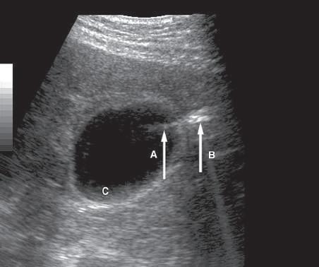
FIG. 1.29 Side Lobe Artifact. Transverse image of the gallbladder reveals a bright internal echo (A) that suggests a band or septum within the gallbladder. This is a side lobe artifact related to the presence of a strong out-of-plane reflector (B) medial to the gallbladder. The low-level echoes in the dependent portion of the gallbladder (C) are also artifactual and are caused by the same phenomenon. Side lobe and slice thickness artifacts are of clinical importance because they may create the impression of debris in fluid-filled structures.
FIG. 1.28 Side Lobes. Although most of the energy generated by a transducer is emitted in a beam along the central axis of the transducer (A), some energy is also emitted at the periphery of the primary beam (B and C). These are called side lobes and are lower in intensity than the primary beam. Side lobes may interact with strong reflectors that lie outside of the scan plane and produce artifacts that are displayed in the ultrasound image (see also Fig. 1.29).
are near the noise levels of the equipment, and considerable skill and experience are needed to adjust instrument settings to display the maximum information with the minimum noise. Poor scanning angles, inadequate penetration, and poor resolution may also result in loss of information. Careless selection of transducer frequency and lack of attention to the focal characteristics of
in what is actually a simple ovarian cyst.
the beam will cause loss of clinically important information from deep, low-amplitude reflectors and small targets. Ultrasound artifacts may alter the size, shape, and position of structures. For example, a multipath artifact is created when the path of the returning echo is not the one expected, resulting in display of the echo at an improper location in the image (Fig. 1.30).
Shadowing and Enhancement
Although most artifacts degrade the ultrasound image and impede interpretation, two artifacts of clinical value are shadowing and enhancement. Again, shadowing results when an object (e.g., calculus) attenuates sound more rapidly than surrounding tissues. Enhancement occurs when an object (e.g., cyst) attenuates less than surrounding tissues. Failure of TGC applied to normal tissue to compensate properly for the attenuation of more highly attenuating (shadowing) or poorly attenuating (enhancing) structures produces the artifact (Fig. 1.31). Because attenuation increases with frequency, the effects of shadowing and enhancement are greater at higher than at lower frequencies. The conspicuity of shadowing and enhancement is reduced by excessive beam width, improper focal zone placement, and use of spatial compounding.
DOPPLER SONOGRAPHY
Conventional B-mode ultrasound imaging uses pulse-echo transmission, detection, and display techniques. Brief pulses of ultrasound energy emitted by the transducer are reflected from acoustic interfaces within the body. Precise timing allows determination of the depth from which the echo originates. When pulsed wave ultrasound is reflected from an interface, the backscattered (reflected) signal contains amplitude, phase, and frequency information (Fig. 1.32). This information permits inference of the position, nature, and motion of the interface reflecting the pulse. B-mode ultrasound imaging uses only the amplitude information in the backscattered signal to generate the image, with differences in the strength of reflectors displayed in the image in varying shades of gray. Rapidly moving targets, such as red cells in the bloodstream, produce echoes of low
amplitude that are not usually displayed, resulting in a relatively anechoic pattern within the lumens of large vessels. Although gray-scale display relies on the amplitude of the backscattered ultrasound signal, additional information is present in the returning echoes that can be used to evaluate the motion of moving targets.16 When high-frequency sound impinges on a stationary interface, the reflected ultrasound has essentially the same frequency or wavelength as the transmitted sound. If the reflecting interface is moving with respect to the sound beam emitted from the transducer, however, there is a change in the frequency of the sound scattered by the moving object (Fig. 1.33). This change in frequency is directly proportional to the velocity of the reflecting interface relative to the transducer and is a result of the Doppler effect. The relationship of the returning ultrasound frequency to the velocity of the reflector is described by the Doppler equation, as follows:
∆FFFFvc RTT =−=⋅⋅ ()2
The Doppler frequency shift is ΔF; FR is the frequency of sound reflected from the moving target; FT is the frequency of sound emitted from the transducer; v is the velocity of the target toward the transducer; and c is the velocity of sound in the medium. The Doppler frequency shift (ΔF) applies only if the target is moving directly toward or away from the transducer (Fig. 1.34A). In most clinical settings the direction of the ultrasound beam is seldom directly toward or away from the direction of flow, and the ultrasound beam usually approaches the moving target at an angle designated as the Doppler angle (Fig. 1.34B). In this case, ΔF is reduced in proportion to the cosine of this angle, as follows:
∆FFFFvc RTT =−=⋅⋅⋅ ()cos2 θ
where θ is the angle between the axis of flow and the incident ultrasound beam. If the Doppler angle can be measured, estimation of flow velocity is possible. Accurate estimation of target velocity requires precise measurement of both the Doppler frequency shift and the angle of insonation to the direction of
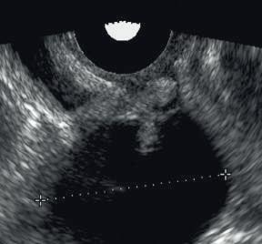
FIG. 1.30 Multipath Artifact. (A) Mirror image of the uterus is created by reflection of sound from an interface produced by gas in the rectum. (B) Echoes reflected from the wall of an ovarian cyst create complex echo paths that delay return of echoes to the transducer. In both examples, the longer path of the reflected sound results in the display of echoes at a greater depth than they should normally appear. In (A) this results in an artifactual image of the uterus appearing in the location of the rectum. In (B) the effect is more subtle and more likely to cause misdiagnosis because the artifact suggests a mural nodule


FIG. 1.31 Shadowing and Enhancement. (A) Uncorrected image of a shadowing breast mass shows that the mass attenuates 25 dB, 15 dB more than the surrounding normal tissue, which attenuates only 10 dB. (B) Application of appropriate time gain compensation (TGC) results in proper display of the normal breast tissue. However, because of the increased attenuation of the mass, a shadow results. (C) Similarly, the cyst attenuates 7 dB less than the normal tissue, and TGC correction for normal tissue results in overamplification of the signals deep to the cyst, producing enhancement of these tissues.
target movement. As the Doppler angle (θ) approaches 90 degrees, the cosine of θ approaches 0. At an angle of 90 degrees, there is no relative movement of the target toward or away from the transducer, and no Doppler frequency shift is detected (Fig. 1.35). Because the cosine of the Doppler angle changes rapidly for angles more than 60 degrees, accurate angle correction requires that Doppler measurements be made at angles of less than 60 degrees. Above 60 degrees, relatively small changes in the Doppler angle are associated with large changes in cosθ, and therefore a small error in estimation of the Doppler angle may result in a large error in the estimation of velocity. These considerations are important in using both duplex and color Doppler instruments. Optimal imaging of the vessel wall is obtained when
the axis of the transducer is perpendicular to the wall, whereas maximal Doppler frequency differences are obtained when the transducer axis and the direction of flow are at a relatively small angle.
In peripheral vascular applications, it is highly desirable that measured Doppler frequencies be corrected for the Doppler angle to provide velocity measurement. This allows comparison of data from systems using different Doppler frequencies and eliminates error in interpretation of frequency data obtained at different Doppler angles. For abdominal applications, angle-corrected velocity measurements are encouraged, although qualitative assessments of flow are often made using only the Doppler frequency shift data.
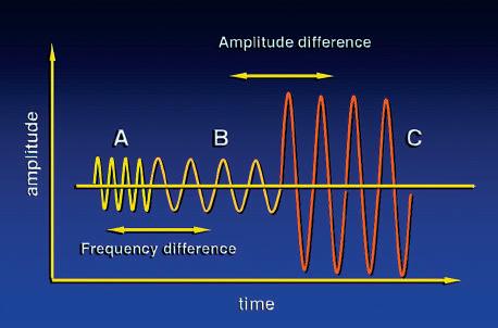
FIG. 1.32 Backscattered Information. The backscattered ultrasound signal contains amplitude, phase, and frequency information. Signals B and C differ in amplitude but have the same frequency. Amplitude differences are used to generate B-mode images. Signals A and B differ in frequency but have similar amplitudes. Such frequency differences are the basis of Doppler ultrasound.
Stationary target: (FR FT) = 0
Target motion toward transducer: (FR FT) > 0
Target motion away from transducer: (FR FT) < 0
FIG. 1.33 Doppler Effect. (A) Stationary target. If the reflecting interface is stationary, the backscattered ultrasound has the same frequency or wavelength as the transmitted sound, and there is no difference in the transmitted frequency (FT) and the reflected frequency (FR). (B) and (C) Moving targets. If the reflecting interface is moving with respect to the sound beam emitted from the transducer, there is a change in the frequency of the sound scattered by the moving object. When the interface moves toward the transducer (B), the difference in reflected and transmitted frequencies is greater than zero. When the target is moving away from the transducer (C), this difference is less than zero. The Doppler equation is used to relate this change in frequency to the velocity of the moving object.
Doppler Signal Processing and Display
Several options exist for the processing of ΔF, the Doppler frequency shift, to provide useful information regarding the direction and velocity of blood. Doppler frequency shifts encountered clinically are in the audible range. This audible signal may be analyzed by ear and, with training, the operator can identify many flow characteristics. More often, the Doppler shift data are displayed in graphic form as a time-varying plot of the frequency
FIG. 1.34 Doppler Equations. The Doppler equation describes the relationship of the Doppler frequency shift to target velocity. (A) In its simplest form, it is assumed that the direction of the ultrasound beam is parallel to the direction of movement of the target. This situation is unusual in clinical practice. More often, the ultrasound impinges on the vessel at angle θ (B) In this case the Doppler frequency shift detected is reduced in proportion to the cosine of θ ΔF, Frequency shift; FR, reflected frequency; FT, transmitted frequency; v, velocity.
spectrum of the returning signal. A fast Fourier transformation is used to perform the frequency analysis. The resulting Doppler frequency spectrum displays the following (Fig. 1.36): • Variation with time of the Doppler frequencies present in the volume sampled