PREFACE
The days of the need for gurus and extensive libraries are behind us. The Internet provides ready and rapid access to knowledge for all. This book offers necessary and sufficient descriptions of salient knowledge that have been tested in traditional classrooms. The book weaves foundations together from disparate disciplines including mathematical sociology, economics, game theory, political science, and biological networks.
Network science is a new discipline that explores phenomena common to connected populations across the natural and man-made world. From animals to commodity trades, networks provide relationships among individuals and groups. Analysis and leveraging connections provide insights and tools for persuasion. Studies in this area have largely focused on opinion attributes. The impetus for this book is a need to examine computational processes for automating tedious analyses and usage of network information for online migration. Once online, network awareness will contribute to improved public safety and superior services for all.
A collection of foundational notions for economic and social networks is available in Jackson (2008). A mathematical treatment of generic networks is present in Easly and Kleinberg (2010). A complementary gap filled by this book is an algorithmic approach. I provide a fast-paced introduction to the state of the art in network science. References are offered to seminal and contemporary developments. The book uses mathematical cogency and contemporary computational insights. It also calls to arm further research on open problems.
The reader will find a broad treatment of network science and review of key recent phenomena. Senior undergraduates and professional people in computational disciplines will find sufficient methodologies and processes for implementation and experimentation. This book can also be used as a teaching material for courses on social media and network analysis, computational social networks, and network theory and applications. Our coverage of social network analysis is limited and details are available in Golbeck (2013) and Borgatti et al. (2013)
Preface
Whereas a teacher is a tour guide to the subject matter, this book is a reference manual. Chapters in each part are related and they progress in maturity. Chapters are semi-independent and a course instructor may choose any order that meets the course objectives. Exercises at the end of each chapter are students’ hands-on projects that are designed for covering learning activities during a semester. Some code is provided in appendices for prototyping and learning purposes only. We do not provide a how-to guide to mainstream social media or codebook for application development that is available elsewhere.
IL 2014
REFERENCES
Borgatti, S., Everett, M., Johnson, J., 2013. Analyzing Social Networks. SAGE Publications. Easly, D., Kleinberg, J., 2010. Networks, Crowds, and Markets. Cambridge University Press Golbeck, J., 2013. Analyzing the Social Web. Morgan Kaufmann Publications Jackson, M., 2008. Social and Economic Networks. Princeton University Press.
Henry Hexmoor Carbondale,
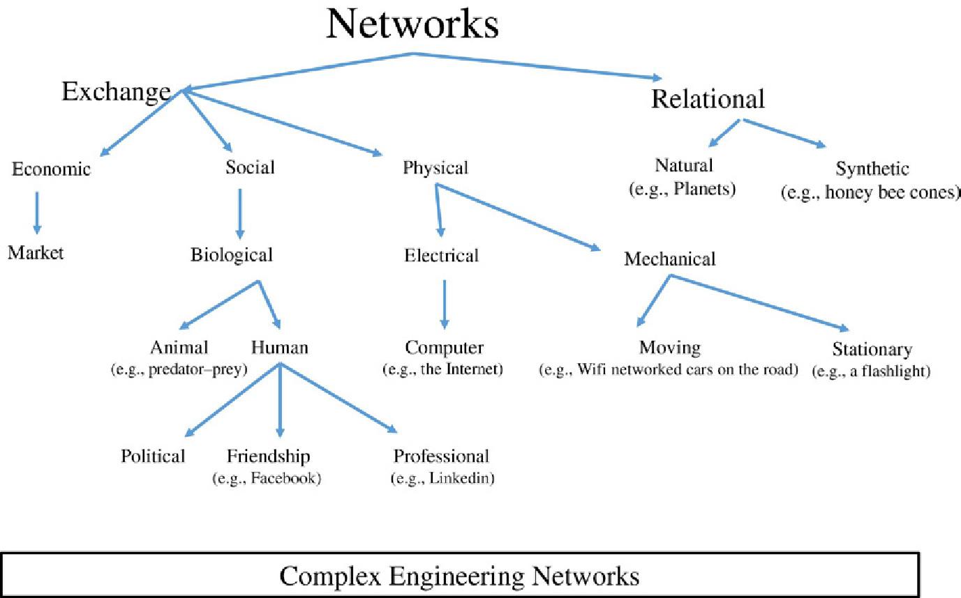
(e.g., trust). Relational networks are inert and merely reflect juxtaposition of nodes. All CENs are exchange networks.
Once a network emerges, we can explore interactions within the network. Strategic interactions involve reasoning and deciding over selection of strategies. They can be modeled with game theory that will be our main focus in Chapter 3.
Network theory is a set of algorithms that codifies relationships among network topology and outcomes, which are meaningful to network inhabitants. There is a movement afoot that codifies network phenomena under the term network science. These phenomena and salient algorithms will be discussed throughout this book.
An Online Social Networking Services (OSNS) creates synthetic networks among people. The salient incentive for using an OSNS is to gain social authority (i.e., legitimacy), which is a form of social power and not generally a measure of vanity. Social authority in social networks is with respect to a group and with respect to specific topics. Therefore, social authority is a relative measure and not an absolute quantity. In Section 1.2, we review a few popular OSNSs from a rapidly growing list (Khare, 2012). Since they provide platforms to create, to share, and/or
Fig. 1.1. A network taxonomy.
to exchange information and ideas in virtual communities, an OSNS is considered to be a medium for social media. There are quantitation schemes over social media, such as Klout, which offers user scores (i.e., a number between 1 and 100). Klout calls influence, which is a measure of a user’s ability to reach one other through an OSNS. This measure is valuable for marketing products online.
In Section 1.3, we review a few popular online bibliographic services (OBS) that house published articles. We return to generic models of networks in Section 1.4. This is followed by a review of popular models of synthetic network generations in Section 1.5. A fully implemented NetLogo model (i.e., code and accompanying descriptions for use) of network generation models and analysis is available in the Appendix.
1.2 ONLINE SOCIAL NE TWORKING SERVICES
Facebook is an OSNS that connects people, organizations, friends, and others who work or live around together. Nodes in a Facebook network can be individuals or organizations. Some of these may be entirely synthetic without real-world humans. The main Facebook tool for connections is friendship. Facebook is used largely for personal and recreational functions. As such, it has filled the social gaps created by physical and psychological dispersion among traditional families and friends. It also serves as a medium that creates relationships that would not otherwise exist.
One Facebook’s feature known as sharing allows adjustments on spread of information (i.e., selecting an audience). Sharing is used to limit who can view posts and photos. It is a three-step process: (1) indicates who you are (i.e., tagging), (2) tells where you live (i.e., adding a location to a post), and (3) manages the privacy right for where you post (i.e., the inline audience selector). Sharing gives users control over their information diffusion, which in turn can yield a measure of social authority. Another Facebook’s like feature provides a directional relationship (i.e., tie, connection, and link) that lends credibility to the item and is proportional to the credibility (i.e., authority) of the endorser.
Twitter is an OSNS that facilitates broadcasts of messages (i.e., tweets). The main twitter tool for connections is the explicit alignments of ideas among people (i.e., following). Twitter can be used by small or large groups to form crowd sourcing. For example, in the small network,
1.4.1
Random Networks
G(n, p) is a random graph model with n nodes where the probability of a pair of nodes in it being linked is denoted by p (Erdős and Rényi, 1959). When p is small, the network is sparsely connected. When p is close to 1/n, the network appears fully connected. When p is almost 1.0, the connectivity among nodes is very high and the network is said to be a giant component. The spread of node degrees for a random graph model (i.e., degree distribution) appears binomial in shape. A closely related model is the random geometric graph G(n, r), where there are n nodes and the distance between a pair of nodes in the graph is less than or equal to r (Penrose, 2003). Contrary to mathematical models, real-world networks exhibit a degree distribution that is unevenly distributed. In the powerlaw distribution, the probability that a node has a degree distribution k (i.e., the number of connected neighbors) is determined by P(k) ≈ kg, where parameter g is typically constrained between 2 and 3, that is, 2 ≤ g ≤ 3. Uneven distribution stems from preferential attachment, where the probability that a new node will attach to a node i is ∑ degree /degree.ij j () () A node degree refers to the node’s number of neighbors. Preferential attachment is commonly found in nature as well as man-made networks such as an economic network (Gabaix, 2009). Random networks are mathematically the most well-studied and well-understood models.
1.4.2 Scale-Free Networks
There is a model based on preferential attachment described by Barabasi and Albert (1999). In this model, a new node is created at each time step and connected to existing nodes according to the “preferential attachment” principle. At a given time step, the probability p of creating an edge between an existing node u and the new node is =+ + pu EV [( degree() 1) /(|| ||)] , where V is a set of nodes and E is the set of edges between nodes. The algorithm starts with some parameters such as the number of steps that the algorithm will iterate, the number of nodes that the graph should start with, and the number of edges that should be attached from the new node to preexisting nodes at each time step. The Barabasi model of network formation produces a scalefree network, a network where the node degree distribution follows a power-law principle. Scale-free networks produce small number of components, small-diameter, heavy-tailed distribution, and low clustering.
each link is chosen uniformly at random (Kleinberg, 2001). Kleinberg studied the model from an algorithmic perspective and showed that, with a high probability, there will be short paths connecting all pairs of nodes and the network will have the lattice-like structure. Kleinberg model does not yield a heavy-tailed degree distribution.
Kleinberg (2000) showed a simple greedy algorithm that can find paths between any source and destination using only n O(log) 2 expected edges. Kleinberg’s algorithm that will be used in this study is based on two parameters: the lattice size and the clustering exponent. Each node u has four local connections, one to each of its neighbors and in addition one long-range connection to some node v, where v is chosen randomly according to the probability proportional to d a, where d is the lattice distance between u and v and a is the clustering exponent.
1.5.2 Barabási and Albert’s Scale-Free Network Generator
Barabási and Albert (1999) discussed the features of the scale-free networks in detail and compared them with the features of other types of networks, for example, small-world networks. Scale-free networks expand continuously by the addition of new vertices, and new vertices attach preferentially to vertices that are already well connected. Most of the real networks are free-scale networks, such as WWW and citation patterns of scientific publications, and both of them follow a power-law distribution (Barabási and Albert, 1999).
Albert and Barabási (2002) showed a comparison between their model and other previously proposed models. They state that other network models start with a fixed number of vertices that are then randomly connected or reconnected without modifying the number of vertices. However, the WWW as an example will grow exponentially in time by addition of any new web page. Also, other network models assume that new edges are placed randomly, that is, the probability of connecting two vertices is independent of the vertices’ degree. However, most of the real networks do not behave like that. They exhibit preferential attachment, that is, connecting two vertices is dependent on the vertices’ degree (Albert and Barabási, 2002).
According to Albert and Barabási (2002), a new node is created at each time step and connected to existing nodes according to the
1.7 CONCLUSIONS
Networks are abundantly around us. They are man-made or naturally occur. They are implicit, hidden, explicit, or articulated. They might be tangible and objectively quantified, or they might be subjective and difficult to quantify. They all tend to change in time, which is the subject of our future chapters on network dynamics.
REFERENCES
Albert, R., Barabási, A.-L., 2002. Statistical mechanics of complex networks. Rev. Mod. Phys. 74, 47–97
Barabási, A.L., Albert, R., 1999. Emergence of scaling in random networks. Science 286, 509–512
Carmona, G., 2012. Existence and Stability of Nash Equilibrium. World Scientific Publishing Company.
Epstein, D., Wang, J., 2002. A steady state model for graph power laws. In: Proceedings of 2nd International Workshop on Web Dynamics. World Scientific Publishing Company.
Erdős, P., Rényi, A., 1959. On random graphs. Publicationes Mathematicae 6, 290–297.
Gabaix, X., 2009. Power laws in economics and finances. Annu. Rev. Econ. 1, 255–294
Jackson, M., 2003. A survey of models of network formation: stability and efficiency. In: Demange, G., Wooders, M. (Eds.), Group Formation in Economics: Networks, Clubs, and Coalitions. Cambridge University Press
Jornet, J.M., Pierobon, M., 2011. Nanonetworks: a new frontier in communications. In: Communications of the ACM. Vol. 54, No. 11. ACM, pp. 84–89.
Khare, P., 2012. Social Media Marketing eLearning Kit For Dummies. Wiley
Kleinberg, J., 2000. The small-world phenomenon: an algorithmic perspective. In: Proceedings of 32nd ACM Symposium on Theory of Computing. ACM, pp. 163–170.
Kleinberg, J., 2001. Small-world phenomena and the dynamics of information. In: Proceedings of the Advances in Neural Information Processing Systems (NIPS), Vol. 14. NIPS.
Kleinberg, J., Tardos, E., 2005. Algorithm Design. Addison-Wesley. Li, W., 1992. Random texts exhibit Zipf’s-law-like word frequency distribution. IEEE Trans. Inf. Theory 38 (6), 1842–1845
McPherson, M., Lovin, L.S., Cook, J., 2001. Birds of a feather: homophily in social networks. Annu. Rev. Sociol. 27, 415–444.
Milgram, S., 1967. The small world problem. Psychol. Today 1 (1), 61–67
Moffett, M., 2010. Adventures Among Ants. University of California Press
Nielsen, M., 2012. Reinventing Discovery: A New Era of Networked Science. Princeton University Press.
Penrose, M., 2003. Random Geometric Graphs. Oxford University Press
Reingold, H., 2000. The Virtual Community. MIT Press.
Seung, S., 2012. Connectome: How Brain’s Wiring Makes Us Who We Are. Mariner Books
Watts, D., Strogatz, S., 1998. Collective dynamic of small-world networks. Nature 393 (6684), 440–442
Geodesic distance, denoted by distanceij, is the number of links in the shortest possible path from node i to node j. Diameter of a network is the largest geodesic distance in the connected network. Reverse distance, denoted by RDij, is distanceij (1 + Diameter). Metrics in Equations 2.1 and 2.2 are adapted from Valente and Foreman (1998):
Structural centrality measures of a node are a host of measures reflecting the structural properties of the links surrounding a focal node. For example, degree centrality of a node is the number of edges incident on the node. Closeness centrality of a node is the average of the shortest path lengths from the node to all other nodes in the network. It is a rather small number in small-world networks (Watts and Strogatz, 1998). Betweenness centrality of a node is a measure of the node’s importance (and possibly influence as discussed in Chapter 7) and is computed using the algorithm shown in Figure 2.1.
Eigenvector centrality measures the centrality of neighbor nodes and has been used as a measure of influence and power, which are discussed later in this book (Bonacich and Lu, 2012). Bonacich developed a beta centrality measure CBC with a parameter a used for adjusting the importance of a node’s degree versus a parameter b for adjusting the importance of the neighbor’s centrality. This is shown in Equation 2.3:
Fig. 2.1. Betweenness value computation.
activities. The documentary filmmaker, Morgan Spurlock, has publicly explored branding on social media. His mission is to raise public awareness and to inform us about the changing landscape of cultural values in the society (e.g., supersize me app).
REFERENCES
Bonacich, P., Lu, P., 2012. Introduction to Mathematical Sociology. Princeton University Press. Borgatti, S., Everett, M., Johnson, J., 2013. Analyzing Social Networks. SAGE Publications Ltd Burt, R., 1995. Structural Holes: The Social Structure of Competition. Harvard University Press. Chiang, M., 2012. Networked Life: 20 Questions and Answers. Cambridge University Press
Freeman, L., 1978. Centrality in social networks: conceptual clarification. Soc. Netw. 1, 215–239
Golbeck, J., 2013. Analyzing the Social Web. Morgan Kaufmann.
Knoke, D., Yang, S., 2007. Social Network Analysis. Sage Publications
Macindoe, O., Richards, W., 2011. Comparing networks using their fine structure. Int. J. Soc. Comput. Cyber-Phys. Syst. 1 (1), 79–97, Inderscience Publishers.
Suthers, D., 2011. Interaction, mediation, and ties: an analytic hierarchy for socio-technical systems. In: Proceedings of the Hawaii International Conference on the System Sciences (HICSS-44). January 4–7, 2011, Kauai, Hawai‘i.
Valente, T., Foreman, R., 1988. Integration and radiality: measuring the extent of an individual’s connectedness and reachability in a network. Soc. Netw. 20 (1), 89–105
Wasserman, S., Faust, K., 1994. Social Network Analysis: Methods and Applications. Cambridge University Press
Watts, D., Strogatz, S., 1998. Collective dynamics of ‘small-world’ networks. Nature 393 (6684), 440–442
EXERCISES
1. How can we track search queries (i.e., say in Google or YouTube) from social network profiles of corresponding users?
2. Describe a network that appears to be but is not a scale-free network.
3. How can beta centrality measure be used to find weakly connected nodes in a network?
4. Modify density metric for weighted networks, that is, networks with links that have weights as strengths of connections.
CHAPTER 3 Network Games
Decision making requires reasoning. Whereas decision theory is about the process of an individual’s reasoning processes when pertinent decision attributes can be independently ascertained, game theory (GT) is about the process of reasoning when pertinent decision attributes include decisions of other individuals (Fudenberg, 1991). The latter is the scenario in networks where all the decisions are interdependent. GT has been a branch of mathematics (Barron, 2008) and has long been used to explain economic decision making in the theories of microeconomics (Mas-Colel et al., 1995). We will briefly introduce GT in Section 3.1 before the discussion of network-relevant applications in Sections 3.2–3.6.
3.1 GAME THEORY INTRODUCTION
A game is a simple tuple 〈I, S, U〉. Here, I is a set of individuals (i.e., players or agents in GT nomenclature). Whereas Si is a nonempty set of actions (i.e., strategies in GT) for agent i, S is a set of all agents’ strategy sets, that is, SSi =Π .
mi: S → R is the utility function (i.e., payoff) for agent i. For a combination of simultaneous decisions, agent i receives a nonnegative reward. For convenience, S i is used to denote the strategies of agents other than agent i.
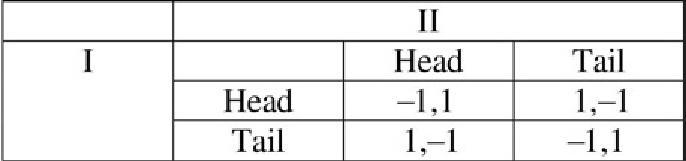
Matching Pennies is a famous zero-sum game of pure conflict with two actions {head, tail}, with a payoff bimatrix shown in Figure 3.1. The minimax theorem guarantees that all zero-sum matrix games are solvable, which means we can determine strategies that maximize player payoffs (Osborne and Rubinstein, 1994).
Many real-world games have action sets with infinite cardinality such as the economic competition among firms deciding on production of product quantities described in Cournot games. In the case of two identical firms and a single product type, Si = [0, ∞], which is the amount of goods that firm i will produce. Payoffs are given by Equation 3.1, where
p is the price of goods as a function of amount of goods produced and ci is the unit cost of the product for firm i:
For Cournot games, it is typical to plot the best responses of two players (i.e., strategies with optimal payoffs for players) with S1 versus S2. In such plots, the point of intersection of the two best response lines denotes the equilibrium point (i.e., stability point) often denoted as S* (i.e., the amount of goods either firm should produce) where neither player will have an incentive to unilaterally abandon the strategy prescribed by the equilibrium.
A famous two-player competitive game is Prisoner’s Dilemma (PD) with prototypical payoffs shown in Figure 3.2 with two strategies of cooperation (C) and defection (D). In PD games, D is the dominant strategy (i.e., the strategy that yields higher payoff for the player) regardless of players’ choices. Often, there are strategies that might be dominated (e.g., suicide would always produce a loss–loss strategy combination in PD) and game analysis often suggests elimination of such strategies (Myerson, 1997). Nash equilibrium (NE) for a game 〈I, S, U〉 is a strategy profile S* ∈ S (i.e., an ideal strategy combination for players) such that for all i ∈ I and for all Si ∈ S, Equation 3.2 holds. NE is a form of equilibrium (i.e., stability). In many competitive games, there are multiple equilibria, among which we must select the most desirable one based on contextual biases (Nisan et al., 2007). A measure of equilibrium efficiency is the Price of Anarchy that is the ratio between the worst and the best equilibria (Roughgarden, 2005).
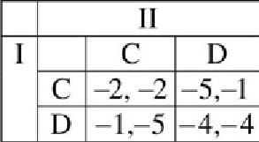
Fig. 3.1 Matching Pennies game payoff bimatrix.
Fig. 3.2. Prisoner’s Dilemma game payoff bimatrix.
In a PD game, if the strategies are selected with equal probability, the expected payoff is computed by Equation 3.3 where both of them are worse off since they earn negative payoffs (i.e., 3.5).
Therefore, our players would not be interested in playing the PD game with equal probabilities. For social optimality bias, payoff pairwise sums of the player pairs would be considered. Whereas (C, C) yields 4, (D, D) yields 8. Therefore, (C, C) would be the socially optimal profile. However, since communication is not allowed in PD and PD is a zero-sum competitive game, social choice is irrelevant.
Thus far, we have considered competition-based games. There is another class of games known as games of coordination where the objective is for players to select a strategy profile such that strategies yield synergistic effects (Hexmoor, 2011). An example is the Battle of the Sexes game with the payoff matrix shown in Figure 3.3. In this game, there are two NEs of (Ballet, Ballet) and (Soccer, Soccer). Expected payoffs for either player who plays each strategy with equal probability are computed by Equation 3.4 that prescribes payoffs of 1/4 for each player. However, players can optimally earn up to (1.5, 1.5) with coordination. In this game, pairs of player payoffs are not zero-sum (i.e., do not sum to zero).
In games that are not zero-sum (e.g., air traffic control and moving heavy objects such as the piano), preplay communication as forms of cooperation, coordination, and negotiation improves payoffs. Therefore, in coordination games, both players win.
Fig. 3.3 Battle of the Sexes payoff bimatrix.