AmericanElectricians’Handbook,SixteenthEdition (AmericanElectrician’sHandbook)16thEdition, (EbookPDF)
https://ebookmass.com/product/american-electricianshandbook-sixteenth-edition-american-electricianshandbook-16th-edition-ebook-pdf/
Instant digital products (PDF, ePub, MOBI) ready for you
Download now and discover formats that fit your needs...
Introduction to 80×86 Assembly Language and Computer Architecture – Ebook PDF Version
https://ebookmass.com/product/introduction-to-8086-assembly-languageand-computer-architecture-ebook-pdf-version/ ebookmass.com
Trapped: Brides of the Kindred Book 29 Faith Anderson
https://ebookmass.com/product/trapped-brides-of-the-kindredbook-29-faith-anderson/
ebookmass.com
80+ Python Coding Challenges for Beginners: Python Exercises to Make You a Better Programmer. No Prior Experience Needed: 80+ Python Challenges to Launch ... Journey. Katie Millie https://ebookmass.com/product/80-python-coding-challenges-forbeginners-python-exercises-to-make-you-a-better-programmer-no-priorexperience-needed-80-python-challenges-to-launch-journey-katie-millie/ ebookmass.com
A Governess Should Never… Deny A Duke: The Governess Chronicles - Book Two Windsor
https://ebookmass.com/product/a-governess-should-never-deny-a-dukethe-governess-chronicles-book-two-windsor/ ebookmass.com
Childhood
and Schooling in (Post)Socialist
Societies: Memories of Everyday Life 1st Edition Iveta Silova
https://ebookmass.com/product/childhood-and-schooling-inpostsocialist-societies-memories-of-everyday-life-1st-edition-ivetasilova/
ebookmass.com
The Ideas of Karl Marx: A Critical Introduction 1st Edition Stefano Petrucciani
https://ebookmass.com/product/the-ideas-of-karl-marx-a-criticalintroduction-1st-edition-stefano-petrucciani/
ebookmass.com
An Introduction to the Gospels and Acts (Essentials of Biblical Studies) Alicia D. Myers
https://ebookmass.com/product/an-introduction-to-the-gospels-and-actsessentials-of-biblical-studies-alicia-d-myers/
ebookmass.com
Finding Joy: Paul's Encouraging Message To The Philippians
John C. Brunt
https://ebookmass.com/product/finding-joy-pauls-encouraging-messageto-the-philippians-john-c-brunt/
ebookmass.com
Fallenness and Flourishing Hud Hudson
https://ebookmass.com/product/fallenness-and-flourishing-hud-hudson/
ebookmass.com
Pragmatic Aspects of Scalar Modifiers: The SemanticsPragmatics Interface 1st Edition Osamu Sawada
https://ebookmass.com/product/pragmatic-aspects-of-scalar-modifiersthe-semantics-pragmatics-interface-1st-edition-osamu-sawada/
ebookmass.com
Control Circuits
Industrial Control Panels
Air-Conditioning and Refrigerating Equipment
Engine-Driven and Gas-Turbine Generators
Division 8 Outside Distribution
Pole Lines: General, Construction, and Equipment
Pole-Line Construction
Pole-Line Guying
Underground Wiring
Grounding of Systems
Division 9 Interior Wiring
General
Open Wiring on Insulators
Concealed Knob-and-Tube Wiring
Rigid-Metal-Conduit and Intermediate-Metal-Conduit Wiring
Cable Pulling Calculations for Raceways
Interior or Aboveground Wiring with Rigid Nonmetallic Conduit
Flexible-Metal-Conduit Wiring
Liquidtight Flexible-Metal-Conduit Wiring
Metal-Clad-Cable Wiring: Types AC and MC
Surface-Raceway Wiring
Electrical-Metallic-Tubing Wiring
Nonmetallic-Sheathed-Cable Wiring
Mineral-Insulated Metal-Sheathed-Cable Wiring
Medium-Voltage-Cable Wiring
Underground-Feeder and Branch-Circuit-Cable Wiring
Interior Wiring with Service-Entrance Cable
Underfloor-Raceway Wiring
Wireway Wiring
Busway Wiring (NEMA)
Cellular-Metal-Floor-Raceway Wiring
Cellular-Concrete-Floor-Raceway Wiring
Wiring with Multioutlet Assemblies
Cablebus Wiring
Cable Trays
General Requirements for Wiring Installations
Crane Wiring
Wiring for Circuits of Over 600 Volts
Wiring for Circuits of Less Than 50 Volts
Wiring for Hazardous (Classified) Locations
Installation of Appliances
Electric Comfort Conditioning
Wiring for Electric Signs and Outline Lighting
Remote-Control, Signaling, and Power-Limited Circuits
Wiring for Special Occupancies
Design of Interior-Wiring Installations
Wiring for Residential Outdoor Lighting
Wiring for Commercial and Industrial Occupancies
Farm Wiring
Solar Photovoltaic Systems
Division 10 Electric Lighting
Principles and Units
Electric-Light Sources
Incandescent (Filament) Lamps
Fluorescent Lamps
High-Intensity-Discharge Lamps
Light-Emitting Diodes (LEDs)
Neon Lamps
Ultraviolet-Light Sources
Infrared Heating Lamps
Luminaires
Principles of Lighting-Installation Design
Tables for Interior Illumination Design
Interior-Lighting Suggestions
Heat with Light for Building Spaces
Street Lighting
Floodlighting
Division 11 Optical Fiber
The Advantages of Fiber Optics
Applications
The Nature of Light
Invisible Light
Transmitting Light through Fibers
Division 12 Wiring and Design Tables
Standard Sizes of Lamps for General Illumination, in Watts
Demand Factors and Data for Determining Minimum Loads
Full-Load Currents of Motors
Capacitor Ratings for Use with Three-Phase 60-Hz Motors
Ampacities of Conductors
Ampacity of Flexible Cords and Cables
Ampacity of Fixture Wires
Ampacity of Aluminum Cable, Steel-Reinforced
Ampacity of Parkway Cables Buried Directly in Ground
Notes to NEC Tubular Raceway and Wire Dimension Tables
Wire-Bending Space, Entries Adjacent to Terminals
Wire-Bending Space, Entries Opposite Terminals
Enclosed Switch Wiring Space
Elevation of Unguarded Parts above Working Space
Ordinary Ratings of Overload Protective Devices, in Amperes
Nonrenewable Cartridge Fuses
Ratings and Number of Overload Protective Devices
Motor Code Letters and Locked-Rotor Kilovolt-Amperes
Maximum Ratings for Motor Branch-Circuit Protection
Conversion Table of Single-Phase Locked-Rotor Currents
Conversion Table of Polyphase Design B, C, D, and E Maximum Locked-Rotor Currents
Horsepower Ratings of Fused Switches
Minimum Branch-Circuit Sizes for Motors
Maximum Allowable Voltage Drop
Graph for Computing Copper-Conductor Sizes According to Voltage Drop
Data for Computing Voltage Drop
Metric Practice
Index follows Division 12
DIVISION 1 FUNDAMENTALS
Conversion Factors
Graphical Electrical Symbols
Principles of Electricity and Magnetism: Units
Measuring, Testing, and Instruments
Harmonics USEFUL TABLES
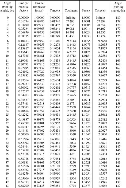
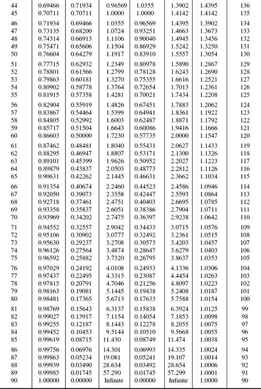
1. Natural Trigonometric Functions
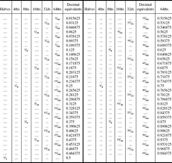
2. Fractions of Inch Reduced to Decimal Equivalents
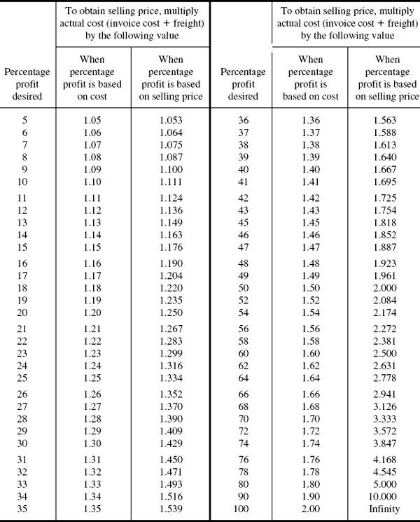
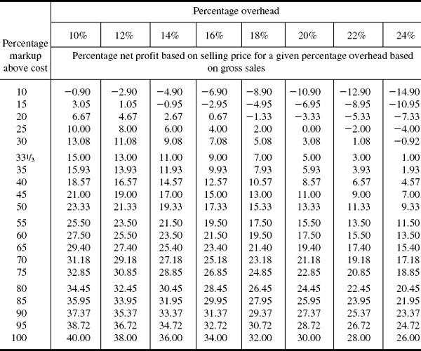
4. Table Showing Percentage Net Profit
NOTE: Minus (–) values indicate a net loss
5. Net profits. In figuring the net profit of doing business, Table 6 will be found to be very useful. The table may be used in three ways, as explained below.
To Determine the Percentage of Net Profit on Sales That You Are Making.
Locate, at the top of one of the vertical columns, your percentage overhead your “cost of doing business” in percentage of gross sales. Locate, at the extreme left of one of the horizontal columns, your percentage markup. The value at the intersection of these two columns will be the percentage profit which you are making.
EXAMPLE If your cost of doing business is 18 percent of your gross sales and you mark your goods at 35 percent above cost, your net profit is 7.93
percent of gross sales, obtained by carrying down from the column headed 18 percent and across from the 35 percent markup.
To
Determine the Percentage Overhead Cost of Doing Business That Would Yield a Certain Net Profit for a Given Markup Percentage. Locate in the extreme left-hand column the percentage that the selling price is marked above the cost price. Trace horizontally across from this value until the percentage net profit desired is located. At the top of the column in which the desired net profit is located will be found the percentage overhead cost of doing business that will allow this profit to be made.
EXAMPLE If the markup is 45 percent and the profit desired is 15 percent, an overhead cost of doing business of 16 percent can be allowed, obtained by carrying across from the 45 percent markup to the 15 percent profit and finding that this column is headed by 16 percent overhead.
To Determine the Percentage That Should Be Added to the Cost of Goods to Make a Certain Percentage Net Profit on Sales. Select the vertical column which shows the percentage cost of doing business at its top. Trace down the column until the desired percentage profit is found; from this value trace horizontally to the extreme left-hand column, in which will be found the markup percentage the percentage to be added to the cost to afford the desired profit.
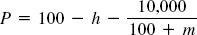
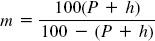
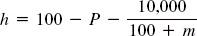
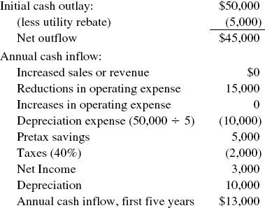
EXAMPLE It is desired to make a 12 percent net profit when the cost of doing business is 20 percent of gross sales. Select the vertical column with 20 percent at its top. Trace down the column to locate the net profit desired of 12 percent. This will be partway between 11.00 and 13.33. Carrying across to the left from these values gives a required markup between 45 and 50, or approximately 47 percent. For values which do not appear in the table, approximate results can be obtained by estimation from the closest values in the table. If more accurate results are desired for these intermediate values, the following formulas may be used:
where m = percentage markup based on cost of goods, h = percentage overhead based on gross sales, and P = percentage net profit based on selling price.
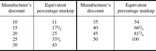
If you sell your goods at the retail list prices set by the manufacturers, you can use the table by converting the trade discount which you receive to an equivalent percentage markup, according to the following table:
Intermediate values may be calculated from the following formula:
where m = percentage markup based on cost of goods and Q = manufacturer’s discount.
6. Accounting for the time value of money. [Adapted with permission from the Jan. 1997 issue of EC&M Magazine, © 1997, Penton Business Media. All rights reserved.]
Many proposals purport to save money over the long term, such as energy management initiatives. Are they actually worthwhile to a customer? A good way to decide is to go into the future and bring the future benefits back to today’s dollars, and compare that result with the project cost. An important tool for this purpose is net present value, because it accounts for the time value of money. To use the tool, you will need to know the project cost, how much money will be saved per year over the project lifetime, and how the customer views his or her financial rate of return.
EXAMPLE
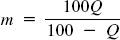
Step 1: Determine the annual cash flow impact of the project
Suppose a group of variable speed drives would cost $50,000 and generate a utility rebate upon completion of $5000. The reduction in electrical expense is projected to be $15,000 per year. Assume the effective rate of taxation is 40 percent and the project could be depreciated (for tax purposes) over five years. Assume no change in the costs of equipment maintenance.
Since there will never be an actual check written for depreciation (the calculation is done for tax impact only) and this is a cash flow analysis, the depreciation goes back in at the end. The result matches the common sense result; the net cash flow is the energy savings ($15,000) reduced by the marginal increase in taxes ($2000). After the first five years, the picture changes due to the fact that, for tax purposes, the equipment is fully depreciated. This means that the taxes go up by $4000 (40 percent of $10,000), reducing the annual positive cash flow to $9000.
Step 2: Determine the hurdle rate
This is the rate of return that the firm needs to realize on the project in order to have it make sense in terms of their own accounting procedure. It consists of the firm’s weighted average cost of capital (WACC) plus a factor reflecting the perceived risk of the proposed project. The point of this part of the analysis is to compare the blended rate of return from the proposed project with the rate of return from other sources of funds the firm may have, both in terms of stock sales and bank financing. Suppose the firm has a million dollar capitalization split 70-30 between shareholder equity (18 percent return expected) and long-term debt (for this example assumed to be 7 percent).
The WACC is $147,000 ÷ $1,000,000 = 14.7 percent. If the risk factor assigned to the project (based on comparable experience and utility rate stability in other locations) were 3.3 percent, then the hurdle rate, the required rate of return, would be 14.7 percent + 3.3 percent = 18 percent. Note that this rate will vary from firm to firm and from time to time based on economic conditions.
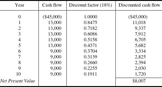
Step 3: Determine the net present value of the project based on the hurdle rate
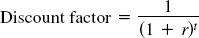
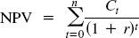
The final step is to calculate what future cash flows are worth in today’s dollars, so a comparison can be made with other projects competing for funding. Year by year, develop a discount rate for that year and multiply it by the expected cash flow. For example, the discount rate for year 3 is 0.6086 (based on an 18 percent return). To see that this comes out correctly, multiply this by 1.18 to get 0.7182 (year 2), and then by 1.18 to get 0.8475 (year 1), and then by 1.18 again to get 1.0000. This result for year 0, which is the present day, shows the calculations are being done correctly. For any future year (t), the discount factor is (where r is the hurdle rate):
(5)
The net present value of all cash flows from the time of project origination onward is the sum of all calculations by year, expressed mathematically as follows where Ct is the cash flow for each future year used in the summation:
(6)
In this example the tabulated results are as follows:
These calculations are tedious to do by hand but there are many computer programs and financial calculators that do the job quickly. The fact that this result is positive shows that it compares well with alternative rates of return and should be strongly considered.
7. Other tools also account for the factor of time in financial management.
For example, the payback time simply divides project cost by marginal revenue. In the example in Step 3, this would be $45,000 ÷ $13,000, or 3.46. Be careful with this tool because it does not take into account ongoing future revenue after the break-even point. A different project with a shorter payback period, but with a shorter useful life, may turn out to be less profitable. For example, suppose a project, also costing $45,000, reduced expenses by $15,000 per year (reducing the payback time from 3.46 years to 3.0 years) but had a useful life of only 4.0 years. The total return would be $60,000, but the drive project financial return, although less at the end of the fourth year, would exceed $60,000 during the fifth year and the profitability would continue to increase for the rest of the project life.
Another tool looks at the net present value, and instead of determining the
discounted value of future savings, calculates the internal rate of return (IRR) for the project. In other words, at what percentage rate of return will the discounted value of all future cash flows just equal the project cost, and therefore make the net present value of the improvements equal zero? In the case of the variable speed drive project in Step. 3, the IRR is just under 24 percent. This is substantially higher than the hurdle rate in that example, but it may be misleading because it assumes reinvestment of all revenues at the same rate of return. Such a rate of return is generally unrealistically high, and the net present value metric is preferred, because it uses actual costs.
CONVERSION FACTORS
(Standard Handbook for Electrical Engineers)
8. Length
1 mil = 0.0254 mm = 0.001 in
1 mm = 39.37 mils = 0.03937 in
1 cm = 0.3937 in = 0.0328 ft
1 in = 25.4 mm = 0.083 ft = 0.0278 yd = 2.54 cm
1 ft = 304.8 mm = 12 in = 0.333 yd = 0.305 m
1 yd = 91.44 cm = 36 in = 3 ft = 0.914 m
1 m = 39.37 in = 3.28 ft = 1.094 yd
1 km = 3281 ft = 1094 yd = 0.6213 mi
1 mi = 5280 ft = 1760 yd = 1609 m = 1.609 km
9. Surface
1 cmil = 0.7854 mil2 = 0.0005067 mm2 = 0.0000007854 in2
1 mil2 = 1.273 cmil = 0.000645 mm2 = 0.000001 in2
1 mm2 = 1973 cmil = 1550 mil2 = 0.00155 in2
1 cm2 = 197,300 cmil = 0.155 in2 = 0.00108 ft2
1 in2 = 1,273,240 cmil = 6.451 cm2 = 0.0069 ft2
1 ft2 = 929.03 cm2 = 144 in2 = 0.1111 yd2 = 0.0929 m2
1 yd2 = 1296 in2 = 9 ft2 = 0.8361 m2 = 0.000207 acre
1 m2 = 1550 in2 = 10.7 ft2 = 1195 yd2 = 0.000247 acre
1 acre = 43,560 ft2 = 4840 yd2 = 4047 m2 = 0.4047 ha = 0.004047 km2 = 0.001562 mi2
1 mi2 = 27,880,000 ft2 = 3,098,000 yd2 = 2,590,000 m2 = 640 acres = 2.59 km2
10. Volume
1 cmil · ft = 0.0000094248 in3
1 cm3 = 0.061 in3 = 0.0021 pt (liquid) = 0.0018 pt (dry)
1 in3 = 16.39 cm3 = 0.0346 pt (liquid) = 0.0298 pt (dry) = 0.0173 qt (liquid) = 0.0148 qt (dry) = 0.0164 L or dm3 = 0.0036 gal = 0.0005787 ft3
1 pt (liquid) = 473.18 cm3 = 28.87 in3
1 pt(dry) = 550.6 cm3 = 33.60 in3
1 qt (liquid) = 946.36 cm3 = 57.75 in3 = 8 gills (liquid) = 2 pt (liquid) = 0.94636 L or dm3 = 0.25 gal
1 liter (L) = 1000 cm3 = 61.025 in3 = 2.1133 pt (liquid) = 1.8162 pt (dry) = 0.908 qt (dry) = 0.2642 gal (liquid) = 0.03531 ft3
1 qt(dry) = 1101 cm3 = 67.20 in3 = 2 pt (dry) = 0.03889 ft3
1 gal = 3785 cm3 = 231 in3 = 32 gills = 8 pt = 4 qt (liquid) = 3.785 L = 0.1337 ft3 = 0.004951 yd3
1 ft3 = 28,317 cm3 = 1728 in3 = 59.84 pt (liquid) = 51.43 pt (dry) = 29.92 qt (liquid) = 28.32 L = 25.71 qt (dry) = 7.48 gal = 0.03704 yd3 = 0.02832 m3 or stere
1 yd3 = 46.656 in3 = 27 ft3 = 0.7646 m3 or stere
1 m3 = 61,023 in3 = 1001 L = 35.31 ft3 = 1.308 yd3
11. Weight
1 mg = 0.01543 gr = 0.001 g
1 gr = 64.80 mg = 0.002286 oz (avoirdupois)
1 g = 15.43 gr = 0.03527 oz (avoirdupois) = 0.002205 lb
1 oz (avoirdupois) = 437.5 gr = 28.35 g = 16 drams (avoirdupois) = 0.0625 lb
1 lb = 7000 gr = 453.6 g = 256 drams = 16 oz = 0.4536 kg
1 kg = 15,432 gr = 35.27 oz = 2.205 lb
1 ton (short) = 2000 lb = 907.2 kg = 0.8928 ton (long)
1 ton (long) = 2240 lb = 1.12 tons (short) = 1.016 tons (metric)
12. Energy Torque units should be distinguished from energy units; thus, foot-pound and kilogram-meter for energy, and pound-foot and meterkilogram for torque (see Sec. 67 for further information on torque).
1 ft · lb = 13,560,000 ergs = 1.356 J = 0.3239 g · cal = 0.1383 kg · m = 0.001285 Btu = 0.0003766 Wh = 0.0000005051 hp · h
1 kg · m = 98,060,000 ergs = 9806 J = 7.233 ft · lb = 2.34 g · cal = 0.009296 Btu = 0.002724 Wh = 0.000003704 hp · h (metric)
1 Btu = 1055 J = 778.1 ft · lb = 252 g · cal = 107.6 kg · m = 0.5555 lb Celsius heat unit = 0.2930 Wh = 0.252 kg · cal = 0.0003984 hp · h (metric) = 0.0003930 hp · h
1 Wh = 3600 J = 2,655.4 ft · lb = 860 g · cal = 367.1 kg · m = 3.413 Btu = 0.001341 hp · h
1 hp · h = 2,684,000 J = 1,980,000 ft · lb = 273,700 kg · cm = 745.6 Wh
1 kWh = 2,655,000 ft · lb = 367,100 kg · m = 1.36 hp · h (metric) = 1.34 hp · h
13. Power
1 g · cm/s = 0.00009806 W
1 ft · b/min = 0.02260 W = 0.00003072 hp (metric) = 0.00000303 hp
1 W = 44.26 ft · lb/min = 6.119 kg · m/min = 0.001341 hp
1 hp = 33,000 ft · lb/min = 745.6 W = 550 ft · lb/s = 76.04kg · m/s = 1.01387 hp (metric)
1 kW = 44,256.7 ft · lb/min = 101.979 kg · m/s = 1.3597 hp (metric) = 1.341 hp = 1000 W
14. Resistivity
1 Ω/cmil · ft = 0.7854 Ω/mil2 · ft = 0.001662 Ω/mm2 · m = 0.0000001657 Ω/cm3 = 0.00000006524 Ω/in3
1 Ω/mil2 · ft = 1.273 Ω/cmil · ft = 0.002117 Ω/mm2 · m = 0.0000002116 Ω/cm3 = 0.00000008335 Ω/in3
1 Ω/m3 = 15,280,000 Ω/cmil · ft = 12,000,000 Ω/mil2 · ft = 25,400 Ω/mm3 · m = 2.54 Ω/cm3
15. Current density
1 A/in2 = 0.7854 A/cmil = 0.155 A/cm2 = 1,273,000 cmil/A = 0.000001 A/mil2
1 A/cm2 = 6.45 A/in2 = 197,000 cmil/A
1000 cmil/A = 1273 A/in2
1000 mil2/A = 1000 A/in2
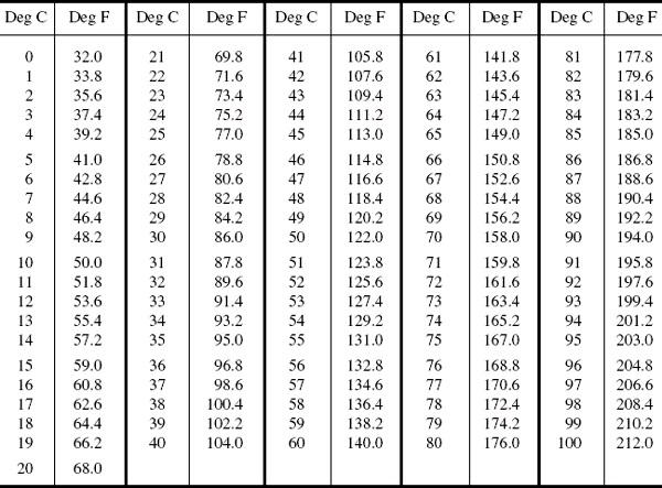
16. Celsius and Fahrenheit Thermometer Scales
For values not appearing in the table use the following formulas:
(7)
(8)
17. Greek Alphabet (Anaconda Wire and Cable Co.)
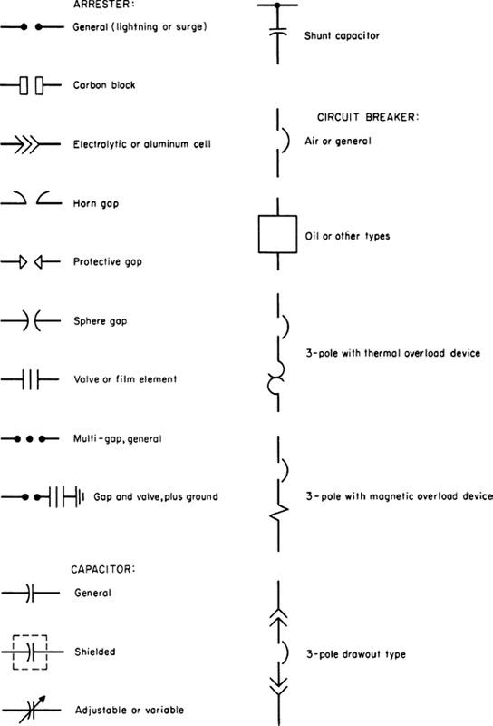
GRAPHICAL ELECTRICAL SYMBOLS
18. Standard graphical symbols for electrical diagrams were approved by the American National Standards Institute (ANSI) on October 31, 1975. The complete list of the standardized symbols is given in the ANSI publication Graphical Symbols for Electrical and Electronic Diagrams, No. ANSI/IEEE 315-1975. A selected group of these symbols for use in one-line electrical diagrams is given in Secs. 19 and 20 through the courtesy of Rome Cable Corporation.
19. Graphical Symbols for One-Line Electrical Diagrams
(From American National Standards Institute ANSI/IEEE 315-1975)