GEOPHYSICS WithMATLABExamples
VOLUME 4
BASHAR
ALSADIK
FacultymemberatBaghdadUniversity–CollegeofEngineering–Iraq(1999–2014) ResearchassistantatTwenteUniversity–ITCfaculty–TheNetherlands(2010–2014) MemberoftheInternationalSocietyforPhotogrammetryandRemoteSensingISPRS
Elsevier
Radarweg29,POBox211,1000AEAmsterdam,Netherlands
TheBoulevard,LangfordLane,Kidlington,OxfordOX51GB,UnitedKingdom 50HampshireStreet,5thFloor,Cambridge,MA02139,UnitedStates
# 2019ElsevierInc.Allrightsreserved.
Nopartofthispublicationmaybereproducedortransmittedinanyformorbyanymeans,electronicor mechanical,includingphotocopying,recording,oranyinformationstorageandretrievalsystem,without permissioninwritingfromthepublisher.Detailsonhowtoseekpermission,furtherinformationaboutthe Publisher’spermissionspoliciesandourarrangementswithorganizationssuchastheCopyrightClearance CenterandtheCopyrightLicensingAgency,canbefoundatourwebsite: www.elsevier.com/permissions
ThisbookandtheindividualcontributionscontainedinitareprotectedundercopyrightbythePublisher (otherthanasmaybenotedherein).
Notices
Knowledgeandbestpracticeinthisfieldareconstantlychanging.Asnewresearchandexperiencebroadenour understanding,changesinresearchmethods,professionalpractices,ormedicaltreatmentmaybecomenecessary.
Practitionersandresearchersmustalwaysrelyontheirownexperienceandknowledgeinevaluatingandusing anyinformation,methods,compounds,orexperimentsdescribedherein.Inusingsuchinformationormethods theyshouldbemindfuloftheirownsafetyandthesafetyofothers,includingpartiesforwhomtheyhavea professionalresponsibility.
Tothefullestextentofthelaw,neitherthePublishernortheauthors,contributors,oreditors,assumeany liabilityforanyinjuryand/ordamagetopersonsorpropertyasamatterofproductsliability,negligenceor otherwise,orfromanyuseoroperationofanymethods,products,instructions,orideascontainedinthe materialherein.
LibraryofCongressCataloging-in-PublicationData
AcatalogrecordforthisbookisavailablefromtheLibraryofCongress
BritishLibraryCataloguing-in-PublicationData
AcataloguerecordforthisbookisavailablefromtheBritishLibrary
ISBN:978-0-12-817588-0
ForinformationonallElsevierpublications visitourwebsiteat https://www.elsevier.com/books-and-journals
Publisher: CandiceJanco
AcquisitionsEditor: AmyShapiro
Editorialprojectmanager: HilaryCarr
Productionprojectmanager: PaulPrasadChandramohan
CoverDesigner: GregHarris
TypesetbySPiGlobal,India
Preface
Therapiddevelopmentindifferentareas ofscienceandtechnologyinthelastdecades transferredengineeringapplicationsintoa newerawherethemajorareasofdesignation,analysis,prototyping,andimplementationarebeingappliedincomputerizedor automatedways.Thismeansthatalarge numberofcomputationsthatwasdifficult orcomputationallyexpensivetoperformin thepastaretodayeasilyhandledandsignificantlyautomatedorprogrammed.
Animportantdivisionofengineering, namely,traditionalsurveyingand/orgeodeticengineering,ispositivelyaffectedby thedevelopmentsoradventsofsatellitenavigation,digitalmapping,informationtechnology,robotics,remotesensing,computer vision,sensorsfusion,andotherfieldsrelated toGeo-wiseapplications.
Accordingly:
– Paper-basedcartographicplottinghas changedtosoft-copyordigitalmapping, webmapping,andgeographic informationsystems(GIS).
– Traditionalphotogrammetryisaffected bycomputerormachinevisiontechniques anddigitalimageprocessingadvents. Further,satelliteremotesensingwith differentimageresolutionsand/or spectralarereplacingtraditionalaerial photographyinmanyapplications.
– Fieldsurveyingequipmentare developingawayfromtraditional theodolitesandelectronicdistance measurements(EDM)towardrobotictotal stationsandglobalnavigationsatellite
system(GNSS)-basedpositioning,asan example.
Hence,theterminologyofsurveyingis changinginmanyeducational,academic, andgovernmentalinstitutionstogeomatics, geoinfomatics,orgeospatialengineering, wherethree-dimensionalobservationsare moreapplied.
Consequently,theauthorcametotheidea ofwritingthisbookthatfocusesontheadjustmentof3Dgeomaticalobservations, whichinspirestraditionaltechniquesand putstheminamodernformsupportedby solvedexamples.Further,thebookisfocusedonpresentingboththeoreticaland practicalcontexttoensureaclearunderstandingofadjustmentcomputationstopic tothereaders.Manynumericalexamplesas mentionedareintroducedandsupportedby MATLABcodestofullyunderstandthetopics. Theauthorshouldmentionthatheisnot aprofessionalprogrammer,andhedeveloped thecodesmainlyforeducationalpurposes. Thebookisintendedforstudents,lecturers, andresearchersinthefieldofgeomaticsand itsdivisions.Thereaderscanfindthefull listofthecodeexamplespublishedinthislink https://nl.mathworks.com/matlabcentral/ fileexchange/70550-adjustment-models-in3d-geomatics.
Thestructureofthebookisdesignedin12 chapterstocoveressentialpreliminaryand advancedadjustmenttopics. Chapter1 introducesstatisticaldefinitions,concepts,and derivations.Themostimportantmethodof theadjustmentusingtheleastsquares
principleanditsmathematicalderivationis alsointroduced.Then,in Chapter2,error propagationtechniqueispresentedandthe variance-covariancematrixofobservations andunknownsisdescribed.Similarly,the preanalysisprocedureispresented.In Chapter3,theadjustmentusingtheconditionequationsandtheobservationequations isintroducedand,attheend,theconceptof thehomogeneousleastsquaresmethodis presented.Forabetterunderstanding,differentadjustmentmodelsareshownin Chapter4 suchasintersectionandresection eitherin2Dor3Dusingobserveddistances, angles,azimuths,differenceinheights,or computationsfromimages.Attheendof Chapter4,animportantcomputationalgeophysicsapplicationisshownofearthquake locationdetermination.Thegeneraladjustmentapproachispresentedin Chapter5 whenthereismorethanoneobservationin themathematicalmodelrelatedtoseveralunknowns.Theimportanttopicofadjustment withconstraintsisintroducedin Chapter6. Threemaintopicsarepresentedinthischapter:adjustmentwithconstraints,adjustment withadditionalparameters,andtheadjustmentwithinnerconstraints(freenets).
Moreadvancedtopicsarepresentedinthe secondhalfofthebook,suchastheunified approachofleastsquaresadjustmentof Chapter7.Thisisanadvancedadjustment techniquewheretheunknownshaveuncertaintiesandarethenprocessedasobservationsinthemodel.
Chapters8and9 presentmorerelatedapplicationsingeomatics,namelythetopicof fitting3Dgeometricprimitivesandthe3D transformationcomputationsrespectively. Thenthebookcontinuestogiveintroduction tootheradvancedtopicssuchastheKalman filterin Chapter10 andthenonlinearleast squaresusingLevenberg-Marquardtin Chapter11.Finally,inthe Chapter12 of thebook,thedetection,identification,and adaptation(DIA)ofthepostadjustment techniquesisintroduced.Thechapterpresentstheblunderdetectionmethodsof datasnooping,robustestimation,andthe randomsampleconsensus(RANSAC).In thebook’sAppendix,aMATLABcodeis givenfortheadjustmentofhorizontal geodeticnetworks.
BasharAlsadik TheNetherlands
StatisticalIntroduction
1.1INTRODUCTION
Ingeomatics,differentkindsofmeasurements(termedas observations inthebook)are applied.Theimperfectionsininstrumentation,weatherconditions,andlimitationsofthe operator0 sskillsproducefieldobservationsthatencompassdifferentkindsoferrors.Accordingly,understandingtheadjustmentofobservationsandtheoryoferrorsareessentialto processandsolvegeomaticalproblems.Becauseweneedconfidenceinappliedengineering orascientificproject,statisticalmeasuresofaccuracy,precision,andreliabilityshouldbe computedand/orstandardized.Itshouldbenotedthatfulfillingtherequiredaccuracystandardswilltakemoretimetoimplement,moreprofessionallabor,advancedinstrumentation, andmorecomputingpower.
Togivereallifeexamplesabouttheimportanceofthischapter’sperspectiveandtopics relatedtoadjustmentofobservations,welisttwoexamplesin
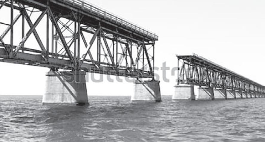
Fig.1.1.Thefirstexample, shownin Fig.1.1A,isaboutanengineeringconstructionproject.Severalquestionscome tomind:Whichendofthebridgeisthecorrectlypositioned/alignedone?Howaccurateit is?Andwhaterrortypemightbeoccurredinthecalculationsandexecutions?
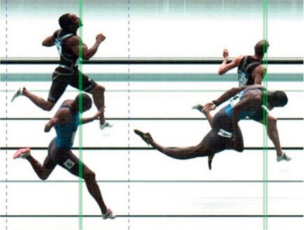
Thesecondexample,shownin Fig.1.1B,showsracingathletesatthefinishlinewherethe timedifferencebetweenthemiswithinfractionsofasecond.Sowhichofthetwocompetitors isthewinner?Howaccurateisthismeasuringimagesystem?Isthecameracalibratedand wellpositioned?
FIG.1.1 (A)Whichendofthebridgeisthecorrectlyalignedone?(B)Whichathleteisthegoldmedalwinner?
Allofthesequestionsaskedof Fig.1.1 canbeansweredwhenweunderstanddifferentconceptsandindicesinadjustmentofobservationsandtheoryoferrorssuchas:accuracy,precision,reliability,calibration,standarddeviation,weightedmean,residualerror,most probablevalue(MPV),redundancy,etc.
1.2STATISTICALDEFINITIONSANDTERMINOLOGIES
• Errors arethedifferencesbetweenobservedvaluesandtheirtruevalues.Anerroriswhat causesvaluestodifferwhenameasurementisrepeated,andnoneoftheresultscanbe preferredovertheothers.Althoughitisnotpossibletoentirelyeliminateerrorina measurement,itcanbecontrolledandcharacterized.Wesummarizedtheterminologies relatedtoerrorsasfollows:
• Grosserrors: Thesearelargeerrors(blunders,mistakes,oroutliers)thatcanbeavoidedin theobservations;however,theydon0 tfollowamathematicalorphysicalmodelandmay belargeorsmall,positiveornegative.Withdevelopmentsininstrumentationand automatedprocedures,themainsourceofgrosserrorsishuman-related,forexample, recordingandreadingerrors,orobservingadifferenttargetthantheintendedone. Carefulreadingandrecordingofthedatacansignificantlyreducegrosserrors.Itshouldbe notedthatsomereferencesdon0 tcountmistakesasanerrortype[1].
• Systematicerrors
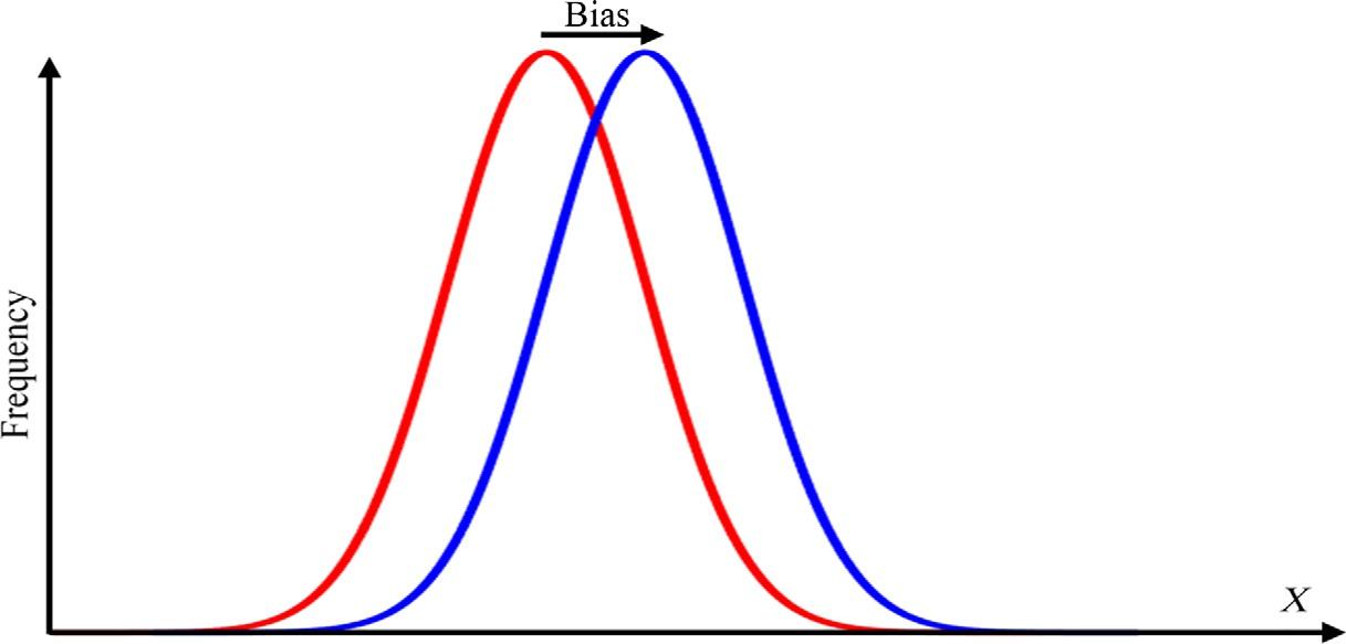
Systematicerrors(orbiaswhenhavingmanyobservations)occurwhenfollowing somephysicalmodelsandthereforecanbechecked.Systematicerrorsareeitherpositiveor negative;usingpropermeasuringprocedurescaneliminatesomeofthem,whereas somearecorrectedbyusingmathematicalmethods.Systematicerrorsourcesare recognizableandcanbereducedtoagreatextentbycarefuldesignationoftheobservation systemandtheselectionofitscomponents.Inpractice,theprocessof calibration of instruments,suchascamerasinphotogrammetry,istodetectandremovesystematic errors.
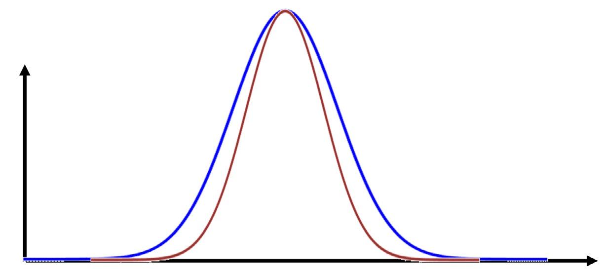
• Fig.1.2 illustratesasystematicerror-freeobservation(redcurve)biasedinacertain directionandamount(thebluecurve).
(A)(B)
Systematicerror(bias)illustration.
• Randomerrors
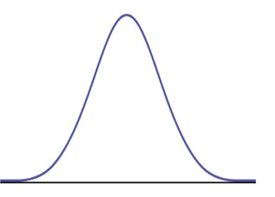
Randomoraccidentalerrorsareunavoidableerrorsthatrepresentresiduals afterremovingallothertypesoferrors.Thistypeoferroroccursinobservationsbecause oflimitationsinthemeasuringinstrumentsorduetolimitationsrelatedtotheoperator, amongotheraffectingundeterminedfactors.Itshouldbenotedthatrandomerrors canbepositiveornegative,andtheydon0 tfollowaphysicalmodel.Therefore,theyare processedstatisticallyusingtheprobabilitytheorembecausethemajorityfollowsnormal distribution.Inrepetitiveobservations,theaverageormeancanbeusedastheMPV. Asshownin Fig.1.3,greaterrandomerrorscauseagreaterdispersionofnormally distributedobservationsaroundthemean.Thedispersionismeasuredbythestandard deviationsatacertainprobabilityaswillbeshowninEq. (1.6).
Observationshavinganormalprobabilitydistribution.(A)Withrandomerrors.(B)Withoutrandom errors.
• Uncertainty
Allobservationshaveuncertainties,whichisarangeofvaluesinwhichthetrueobservationcouldlie.Anuncertaintyestimateshouldaddressbothsystematicandrandomerrors,andthereforeisconsideredthemostpropermeasureofexpressingaccuracy. However,inmanygeomaticsproblems,thesystematicerrorisdisregarded,andonlyrandomerrorisincludedintheuncertaintyobservation.Whenonlyrandomerroriscounted intheuncertaintyevaluation,itisanexpressionoftheprecisionoftheobservation.
FIG.1.2
The normal distribution of X without random errors
The normal distribution of X with random errors
FIG.1.3
• AccuracyandPrecision
Accuracy istheclosenessbetweenanobservedvalueanditstruevalue(trueness).When theobservationsfollownormalprobabilitydistribution,accuracycanbeillustratedas shownin Fig.1.4.Therefore,removingsystematicerrorsimprovesaccuracy.
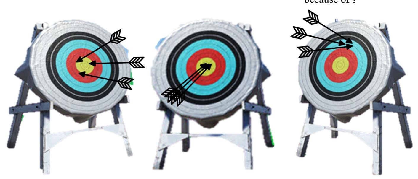
Precision istheclosenessbetweenindependentobservationsofaquantityunderthesame conditions(Fig.1.4).Itisameasureofhowwellavalueisobservedwithoutreferencetoa theoreticalortruevalue.Thenumberofdivisionsonthescaleofthemeasuringdevicegenerallyaffectstheconsistencyofrepeatedobservationsand,therefore,theprecision.Because precisionisnotbasedonatruevalue,thereisnobiasorsystematicerrorinthevalue,but ratheritdependssolelyonthedistributionofrandomerrors.Theprecisionofameasurementisusuallyindicatedbytheuncertaintyorfractionalrelativeuncertaintyofavalue. Anotherusefulillustrationabouttheconceptofprecisionandaccuracyisshownin Fig.1.5 usinganarcherytargetfieldinthreecases.
FIG.1.4 Accuracyandprecision.
FIG.1.5 Relationbetweenaccuracyandprecision.
Therefore:
– Reducingsystematicerrorsimprovesaccuracy.
– Reducingrandomerrorsimprovesprecision.
Anincorrecttermissayingthatyoucanreducerandomerrorsbychoosing amoreaccurate measuringdevice.Thecorrecttermistosay amoreprecisemeasuringdevice.Forexample,smaller scaledivisionsmeanasmallerspread,whichleadstohigherprecisionwhereasamoreaccuratedevicewouldbeonethatreadstruevalues.
• Reliability
Reliabilityisanimportantterminadjustmentcomputations.Reliabilityreferstothedegreeofconsistency,orreproducibility,ofobservations.Inotherwords,reliabilitydefines byhowmuchtheadjustedobservationsmustagreewithreality.Itshouldbenotedthat errorsinobservationscanresultinpoorreliability. Fig.1.6 showsexamplesofreliable andunreliableobservations.ThethreelinesAB,CD,andEFintersectatpointP;however, theleftplotshowslessreliableobservationswhereastherightplotshowsreliableobservationswherethethreelinesintersectalmostexactlyatP.
(Left)lessreliableobservations;(right)reliableobservations.
• Residualerror
Residualerror v meansthedifferencebetweenthetruevalueanditsobservedvalue. However,becausethetruevalueisimpossibletoreach,itisstatisticallycompensated bythe MPV.Therefore:
Itshouldbenotedthatthe MPV valueofrepetitiveobservationsisthearithmeticmean, whereasforotherobservations,itistheoptimalvaluethatofferstheminimalofthesquared residualerrors.Thisconceptwillbeexplainedintheleastsquaresprincipleof Section1.7.Itis importanttonotethatthe MPV intheconceptoftheleastsquaresrepresentstheadjusted valuesofobservations.Fornonlineargeomaticalproblems,theadjustedvaluesarecomputed byrunningthesolutionwithinitialvalues.Accordingly:
FIG.1.6
1.3STATISTICALINDEXES
• Arithmeticmean x:whenobservingaquantity x for n timesunderthesameconditions,the mean x iscomputedasfollows:
• Variance σ 2:thetheoreticalmeanofthesquaredresidualerrorsthatcanbecomputedas follows:
Thedenominator n 1iscalledthe redundancyr orthe degreeoffreedom.Theminimum observationsweneedtodeterminethevarianceisonly1value,whichistermedas no;accordingly,therestoftheobservationsareredundant,and r canbeformulatedas:
• Standarddeviation σ :thesquarerootofthevariancethatexpressesbyhowmuchthe observationsdifferfromthe MPV orthemeanvalue.Further,itisameasureofhowspread outtheobservationsare.Therefore,standarddeviationisanexpressionofprecision computedas:
Whenthereferencevaluesareavailable,thestandarddeviationistermedasthe RootMean SquaredError (RMSE),whichindicatesbyhowmuchtheobservedorderivedquantitiesdeviatefromthereference(true)values.
• Standarderror σx :representsthestandarddeviationofthemean,whichiscomputedas:
EXAMPLE1.1
Given
AbaselineABisobservedinmeters10timesasfollows:
Required
26.34226.34926.35126.34526.348
26.35026.34826.35226.34526.348
Findthe MPV,thestandarddeviation,andstandarderroroflineABtothenearestmm.
Solution
The MPV forrepetitiveobservationsisthemean:
Thestandarddeviationiscomputedas:
Thestandarderroriscomputedas:
Then
1.4NORMALDISTRIBUTIONCURVE
Inliteraturerelatedtogeomatics,itispresentedthatallobservationstakenbysurveyors, suchasobserveddistancesandangles,orobservationsappliedbyphotogrammetristsand geodesistscomplywithorfollowprobabilitylows.Further,randomerrorsthatexistinthe observationsarenormallydistributed(Example1.2).Accordingly,statisticaltechniques canbeappliedinpostprocessingandanalysisoftheobservations.
Thenormaldistributioncurveorthegaussiancurvecanbecalculatedandthenplotted usingthefollowingEq. (1.9).
where
y:thenormalprobability,
K ¼ nI σ 2π p , h2 ¼ 1 2σ 2 calledtheaccuracyindex,
v:theresidualerror,
σ :thestandarddeviation,
I:anyselectedintervaloftheresidualerrors, e:exponentialfunction.
EXAMPLE1.2
Given
Anangleisobserved50timesindegreesasillustratedin Table1.1:
TABLE1.1 MeasuredAngle
40.342937040.341490840.337339040.336326940.340057740.3441110
40.341491540.337323740.335234940.339877340.341659440.3419747
40.336662040.338515440.341211540.343357940.345241240.3384449
40.336543940.338117940.340168540.339742940.337749040.3466756 40.342422240.343478740.340189240.345627040.339416140.3384703
40.338226340.342224240.337428940.340199740.340215240.3411796
40.343206240.340539040.341966540.339315440.340931640.3441452
40.336849540.343576640.341385640.336439840.341194740.3443333
40.337197640.3395228
Required
– Computethe MPV oftheangleanditsstandarddeviation.
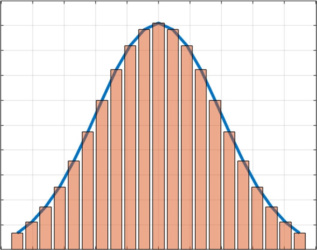
– Computeandplotthenormalprobabilitydistributioncurveofresidualerrors.
Solution
The MPV oftheangleissimplythearithmeticmean,therefore: MPV ¼ meanofangles ¼ 40.3404387degrees
whereasthestandardsdeviationiscomputedas:
Tocomputetheprobability y ofthenormaldistributioncurve,thefollowingelementsare computed:
Thecomputedresidualsaregroupedbetweentwomaximum/minimumlimitsof 22.4500 .Then, tohave20regularintervalsfortheplottingissue,intervalIiscomputedtobe2.24500 asillustratedin thefollowingMATLABcode.
Table1.2.illustratesthedetailsofthecomputationstorelatetheresidualerrorsinsecondstothe computedprobability y ofthenormaldistributioncurve.
TABLE1.2 ComputedProbabilityoftheMeasured Angle
22.45504.002.6113.600.33
20.20408.042.118.250.55
17.96322.561.675.310.86
15.72247.121.283.601.26
13.47181.440.942.561.78
11.22125.890.651.922.37
8.9880.640.421.523.00
6.7445.430.231.263.61
4.4920.160.101.114.10
2.245.020.031.034.42
0.000.000.001.004.55
2.245.020.031.034.42
4.4920.160.101.114.10
6.7445.430.231.263.61
8.9880.640.421.523.00
11.22125.890.651.922.37
13.47181.440.942.561.78
15.72247.121.283.601.26
17.96322.561.675.310.86
20.20408.042.118.250.55
22.45504.002.6113.600.33
Thenthenormaldistributioncurveandhistogramcanbeplottedasshownin Fig.1.7
–25–20–15–10–50 Residualssec. Probability
FIG.1.7 Thenormaldistributionofresidualsinseconds.
MATLABcode
%%%%%%%%%%%%%%%%%%%%%%%%%%%%%%%%%%%%%%%%%%%%%%%%%%%%%%%%%%%%%%%%%%%%%%%%
%%%%%%%%%%%%%%%%%chapter1-example1.2%%%%%%%%%%%%%%%%%%%%%%%%%%%%
%%%%%%%%%%%%%%%%%%%%%%%%%%%%%%%%%%%%%%%%%%%%%%%%%%%%%%%%%%%%%%%%%%%%%%%% clc,clear,closeall
%%%%%%%%%%%%%createnormallydistributedobservedangles%%%%%%%%%%%%%%%%% ang=40.34+10*(randn(50,1)/3600);%%addingrandomnormalnoiseof10sec.
%%%%%%%%%%%%%%%%%%%%%%%%%%%%%%%%%%%%%%%%%%%%%%%%%%%%%%%%%%%%%%%%%%%%%%%%%%% %%computeresiduals resid=3600*(ang-mean(ang)); Resid=unique(round(resid*100)/100); m=max(abs(Resid));%%makeequalintervals I=((2*m)/20)%20intervals%canbechangedbytheuser v=-m:I:m;v=round(v’*100)/100;%sampletheresidualsequallyinseconds v2=round(v.^2*100)/100;%squaredresiduals sigma=std(ang);sigma=sigma*3600;%standarddeviationinseconds n=size(ang,1);%totalnumberofobservations
k1=(n*I)/(sigma*sqrt(2*pi));%k1ofthenormalprobab.distribution k2=1/(2*sigma^2); %k2ofthenormalprobab.distribution
k2v2=round(k2*v2*100)/100; exp_k2v2=round(exp(k2v2)*100)/100; y=round((k1./exp_k2v2)*100)/100;%Yprobability
%%%%%%%%%%%%%%%%%%%%%%%%%%%%%%%%%%%%%%%%%%%%%%%%%%%%%%%%%%%%%%%%%%%%%%%%%% plot(v,y,’-’,’linewidth’,3);holdon;%plotthenormalcurve
xlabel(’RESIDUALSsec.’)
ylabel(’PROBABILITY’)
gridon
disp(’SUMMARIZEDCALCULATIONS’)
disp(’-————————————————————’)
T=table(v,v2,k2v2,exp_k2v2,y)
%%%%%%%%%%%%%%%%%%%%%%%%%%%%%%%%%%%%%%%%%%%%%%%%%%%%%%%%%%%%%%%%%%%%%%%%%% bar(v,y);alpha(.5);%plotthebars
%%%%%%%%%%%%%%%%%%%%%%%%%%%%%%%%%%%%%%%%%%%%%%%%%%%%%%%%%%%%%%%%%%%%%%%%%%% 1.5CUMULATIVEDISTRIBUTIONFUNCTION
Asetofobservationsthatarenormallydistributedcanberepresentedasahistogramor distributioncurveasshowninExample1.2.
Ontheotherhand,the CumulativeDistributionFunction (CDF)showsthepercentageor relativecountofthesortedobservationvaluesovertheobservationsthemselves[2].This is,infact,theintegralofthenormaldistributionhistogram.
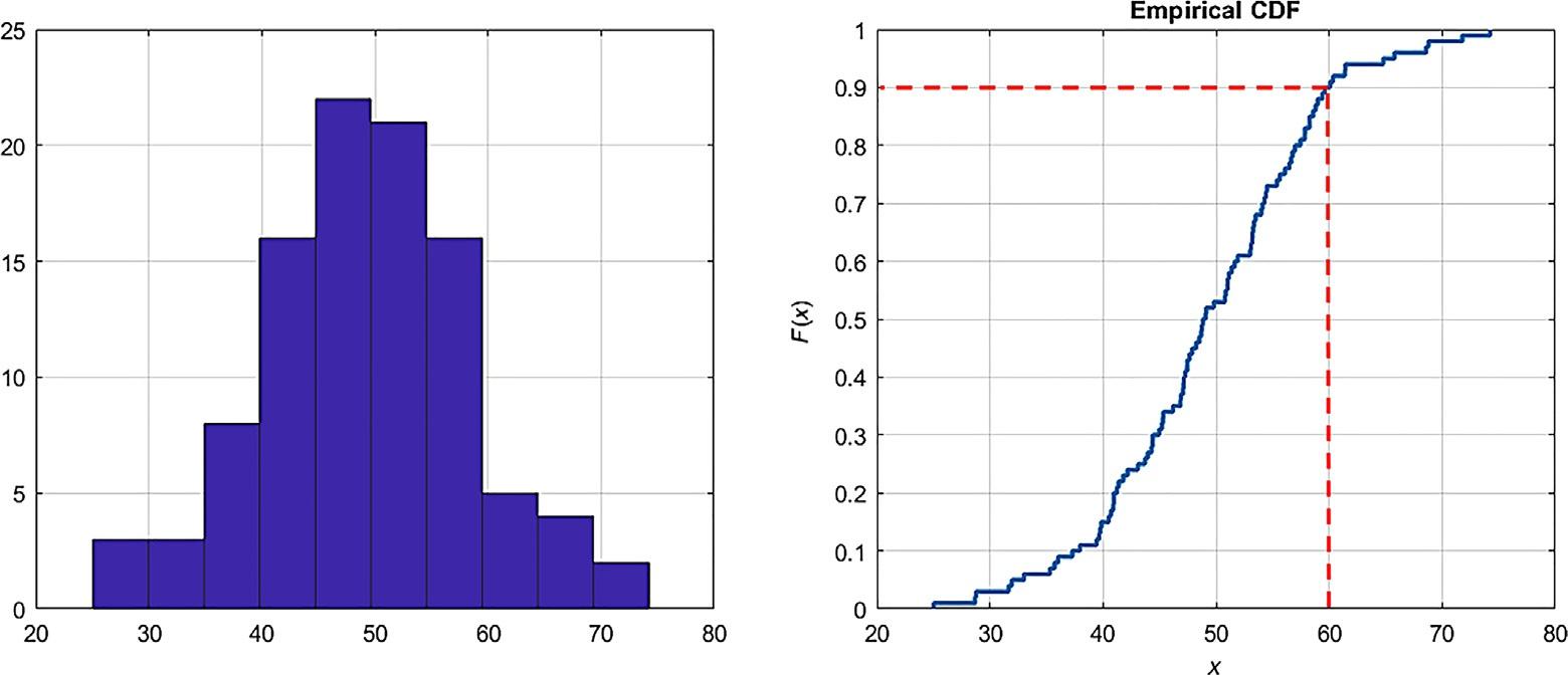
Let’sassumewehave100observationsofananglewherethemeanis50degreeswitha precisionof 10degrees.Wecanrepresenttheobservedvalueseitherinahistogramorin aCDFplotasfollows:
MATLABcode
%anglexbiasedrandomly
x=randn(100,1)*10+50 subplot(1,2,1) hist(x) subplot(1,2,2) cdfplot(x)
TheCDFplotin Fig.1.8Bexplainsthat90%oftheobservedanglesarelessthanorequalto 60degrees.Thispropertyiseasytointerpretevenforanonprofessional.Therefore,keyvalues suchasminimum,maximum,median,percentiles,etc.canbedirectlyreadfromthediagram. Accordingly,CDFisanefficientdescriptionforrandomvariableuncertaintyandisauseful toolforcomparingthedistributionofdifferentsetsofdata.
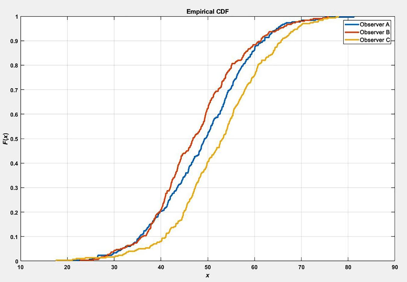
Let’sassumethatthreeobserversA,B,andCmeasuredthesameangle300timeseach.To comparetheskillofthethreeobserversinobservingtheangle,wecanusetheCDFplotas shownin Fig.1.9.
FIG.1.8 (A)Normaldistributionhistogram,(B)ThecorrespondingCDFplot.
FIG.1.9 TheCDFplotsoftheangleobservedbythreesurveyors.
MATLABcode clear;clc;closeall %anglebiasedrandomly A=randn(300,1)*10+50 hA=cdfplot(A);holdon set(hA(:,1),’Linewidth’,3); B=randn(300,1)*10+48
hB=cdfplot(B);holdon set(hB(:,1),’Linewidth’,3);
C=randn(300,1)*10+53
hC=cdfplot(C);holdon set(hC(:,1),’Linewidth’,3); lgd=legend(’observerA’,’observerB’,’observerC’,’fontsize’); lgd.FontSize=12; 1.6THEPROBABLEERRORANDLEVELSOFREJECTION
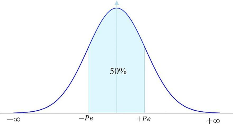
Theprobableerror Pe_50% isdefinedasthe50%orequalprobabilitythatatrueerrorcan arise.Inotherwords,50%probabilityoccurswhen j vi j > Pe_50% and50%when j vi j < Pe_50% as shownin Fig.1.10
FIG.1.10 The50%probableerror.
Foragroupofobservations,the50%probableerroristhemedianofresidualerrorsafter sortingtheminascendingordescendingorder,andthereforeitissometimestermedasthe medianabsolutedeviation (MAD)(Chapter12).However,byusingthisapproach,theprobable errorisnotsensitivetogrosserrorsasshowninthefollowingillustrationswheretheprobable erroris500 forbotherrorsetsdespitetheexistenceofgrosserrorof9400 .
Statistically,torelatetheprobableerror Pe_50% withthestandarddeviations,wecanapply thefollowingderivationbytheintegrationofthenormaldistributioncurveequationas:
Accordingly,theprobableerrorisevaluatedas:
where σ isthestandarddeviationand v isresidualerror. Applyingthesamederivationprocedure,wecancomputetheprobableerrorforanygiven standarddeviation.Hence,theprobableerrorfortherange σ isfoundtobe:
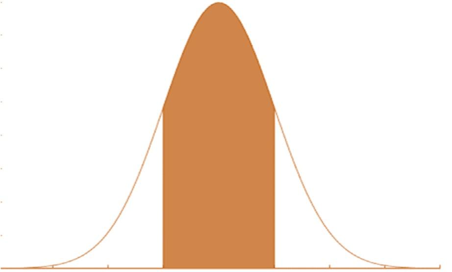
Therefore,theprobableerrorbetween σ and+ σ is68%ofthetotalareaofthenormal curveasshownin Fig.1.11.Asanillustration,whenalinelengthisobservedwithaprecision of 0.06m,itmeansthereisaprobabilityof68%thatthetrueerrorofobservationsisequalto orlessthan 0.06m.
point
Inflection point
FIG.1.11 Probableerrorintherangeof σ
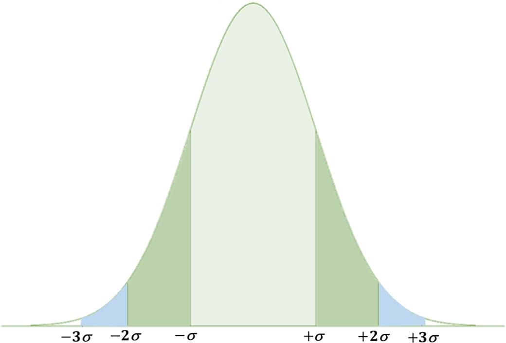
Inthesamemanner,theprobableerroroftheintervals 2σ and 3σ arecomputedas showninEq. (1.13) and Fig.1.12.
FIG.1.12 Differentstandarddeviationslimitsofthenormaldistributioncurve.
Usually,thethresholdof3σ isusedforblenderdetection.Accordingly,residualsfallingat anyofthetwoendsofthenormalcurveinthe1%marginalareaoutsidethe99%ofconfidence areassumedtobeblunders. Table1.3 illustratesdifferentprobabilitypercentagesandtheassociatedstandarddeviationthresholdsthatcanbeadoptedforblunderdetectionorother postanalysisapplications.
TABLE1.3 TheRelationBetweenProbableErrorsandStandardDeviations
1.7PRINCIPLEOFLEASTSQUARESADJUSTMENT
NormaldistributioncurveasmentionedinEq. (1.9) is:
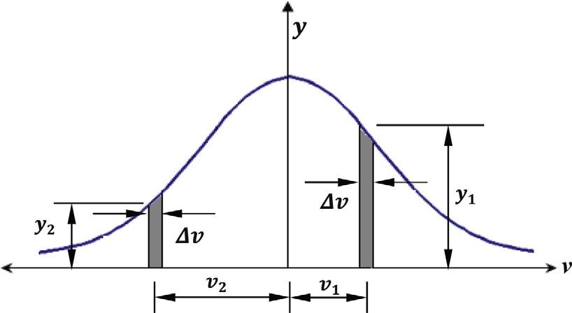
Theprobabilityofoccurrenceof vi ismathematicallyexpressedasarectangularslicearea underthenormaldistributioncurveasshownin Fig.1.13 withavalueof y1 Δ vi.Accordingly, theprobability Pvi ofhavingmoreresidualerrors v1, v2, … vn intheobservationsare:
FIG.1.13 Theprobabilityoferror vi occurrence.
Hence,theprobabilityoftheoccurrenceoftheerrorsaltogetheristhemultiplicationofthe involvedprobabilitiesas:
orsimplifiedas:
FIG.1.14 Theinverserelationbetween x and e x .
Theinverserelationbetweenexponentialfunction e x andvariable x isillustratedin Fig.1.14 wheretheminimalvalueof x isattainedwhen e x isatmaximum.
Accordingly,referringbacktoEq. (1.16),themaximumprobabilityvaluecanbeattained whenthesumofthesquarederrors(v1 2 + v2 2 + … + vn 2 )isatminimum,whichistheprincipleof leastsquaresadjustmentmethod.
orinmatrixformsas:
Insummary,the MPV (adjustedvalue)isthevaluewhenitssumofsquaredresidualerrors isatminimum.Theleastsquaresmethodisconsideredthemostcommonandrobust statistical-basedmethodofadjustmentofobservations.
EXAMPLE1.3
Provethatthearithmeticmean x representsthe MPV oftherepetitiveobservationsofaquantity xi usingtheprincipleofleastsquares.
Solution
The MPV intheconceptofleastsquaressatisfiestheminimumofsquaredresidualerrorsand, accordingly,ifaquantity xi isobserved n timesinthesameprecision,wecanputforththefollowing formulation:
where v ’ s aretheresidualerrors.BysubstitutingEq. (1.19) inEq. (1.17) ofleastsquaresmethod, wegetthefollowing:
Hence,deriving P v 2 withrespecttothemean x:
2
Aftersimplification,wegetthefollowing:
or
Then
1.8WEIGHTEDOBSERVATIONS
Inpractice,theobservationsarenotacquiredinthesameprecisionbecauseofdifferent observers,instruments,dates,dissimilarquantities,etc.
Therefore,thedifferenceinweights w shouldbeconsideredtogiverealisticadjustment results.Whenevertherequiredprecisionishigher,theobservationweightishigher.Onthis basis:
•Theweightisinverselyproportionaltostandarddeviationsofobservationsas:
•Theweightisinverselyproportionaltoobservedlength(asinlevelingnetworks):
•Theweightisconverselyproportionaltothenumberofobservations n as:
TheleastsquaresprincipleofEq. (1.17) canbeupdatedbyconsideringtheweightsas:
Further,thearithmeticmean x withtheconsiderationofweightswillbecomputedas follows:
ThestandarddeviationoftheweightedmeanisalsoupdatedcomparedtoEq. (1.8) tothe followingform:
Tocomputethestandarddeviationforoneobservation xi thathasaweightof wi,weusethe followingequation:
It’sworthmentioningthatEqs. (1.27)and(1.28) canbeprovenbyapplyingthepropagation oferrorslawof Chapter2
EXAMPLE1.4
Given
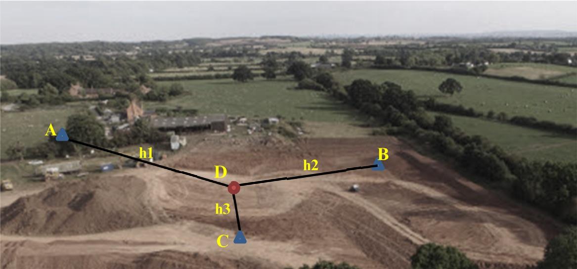
•Threeheightbenchmarks A, B,and C (Fig.1.15)as: HA ¼ 10.00m, HB ¼ 11.01m, HC ¼ 12.05m.
•Theobserveddifferenceinelevationsandlevelinglengthsaregivenas:
ΔHA ¼ 4 00m, LAD ¼ 1 10km
ΔHB ¼ 3:00m, LAD ¼ 0:75km
ΔHC ¼ 2 00m, LAD ¼ 0 50km
FIG.1.15 LevelingnetworkofExample1.4.
Required
ComputetheadjustedheightofstationDanditsstandarddeviationtothenearestcm.
Solution
Theweightedmeanrepresentsthe MPV oftheheightandaccordinglyweightscanbecomputed fortheobserveddifferencesinheightsfromthethreebenchmarksA,B,andCtotheunknownstationD.Asmentioned,weightsareinverselyproportionaltolevelinglinelengthsandthereforethe weightsarecomputedas:
TheestimatedheightofDfromeverylevelinglineisevaluatedasfollows:
Then
Tocomputethestandarddeviationoftheweightedmean,wefirstneedtocomputetheresiduals andthevarianceofunitweightasfollows:
Hence,thestandarddeviationoftheweightedmeaniscomputedas:
ThenthefinaladjustedheightofstationDis14.03m 16mm.
MATLABcode
%%%%%%%%%%%%%%%%%%%%%%%%%%%%%%%%%%%%%%%%%%%%%%%%%%%%%%%%%%%%%%%%%%%%%%%%%%% %%%%%%%%%%%%%%%chapter1-example1.4%%%%%%%%%%%%%%%%%%%%%%%%%%%%%%%%%%% %%%%%%%%%%%%%%%%%%%%%%%%%%%%%%%%%%%%%%%%%%%%%%%%%%%%%%%%%%%%%%%%%%%%%%%%%%% clc,clear,closeall
%Given dha=4;dhb=3;dhc=2;%diff.inheight
La=1.1;Lb=.75;Lc=.5;%length
Ha=10;Hb=11.01;Hc=12.05;%absoluteheight
%%%%%%%%%%%%%%%%%%%%%%%%%%%%%%%%%%%%%%%%%%%%%%%%%%%%%%%%%%%%%%%%%%%%%%%%%%%
%weights
wa=1/La;wb=1/Lb;wc=1/Lc; %initialheightofD
Hd1=Ha+dha; Hd2=Hb+dhb; Hd3=Hc+dhc;
%weightedmean
M=round(100*(Hd1*wa+Hd2*wb+Hd3*wc)/(wa+wb+wc))/100; %thevarianceofunitweight va=(Hd1-M)*1000; vb=(Hd2-M)*1000; vc=(Hd3-M)*1000; sigma=(wa*va^2+wb*vb^2+wc*vc^2)/(3-1); %%%standarddeviationoftheweightedmean s_M=round(sqrt(sigma/(wa+wb+wc)))
%%%%%%%%%%%%%%%%%%%%%%%%%%%%%%%%%%%%%%%%%%%%%%%%%%%%%%%%%%%%%%%%%%%%%%%%%% disp(’Result’) [num2str(M),’m’,char(177),num2str(s_M),’mm’]
%%%%%%%%%%%%%%%%%%%%%%%%%%%%%%%%%%%%%%%%%%%%%%%%%%%%%%%%%%%%%%%%%%%%%%%%%%
EXAMPLE1.5
Given
Threeangles A, B,and C areobservedinatriangulartraversebytwoobserversasfollows (Table1.4):
TABLE1.4 TheMeasuredAnglesbytheTwoObservers
Required
Computetheadjustedangles A, B,and C usingtheweightedmeancomputations.
Solution
Theanglesshouldbefirstadjustedtothegeometricconditionofthesumoftriangleanglesto180 asillustratedin Table1.5.