With Early Release eBooks, you get books in their earliest form—the author’s raw and unedited content as they write—so you can take advantage of these technologies long before the official release of these titles.
If you have comments about how we might improve the content and/or examples in this book, or if you notice missing material within this chapter, please reach out to Pearson at PearsonITAcademics@pearson.com
Contents
Chapter 1 Introduction to Data Structures
Chapter 2 Big-O Notation and Complexity Analysis
Chapter 3 Arrays
Chapter 4 Linked List
Chapter 5 Stacks
Chapter 6 Queues
Chapter 7 Trees
Chapter 8 Binary Trees
Chapter 9 Binary Search Trees
Chapter 10 Heaps
Chapter 11 Hashtable (aka Hashmap or Dictionary)
Chapter 12 Trie (aka Prefix Tree)
Chapter 13 Graphs
Chapter 14 Introduction to Recursion
Chapter 15 Fibonacci and Going Beyond Recursion
Chapter 16 Towers of Hanoi
Chapter 17 Search Algorithms and Linear Search
Chapter 18 Binary Search
Chapter 19 Binary Tree Traversal
Chapter 20 Depth-First Search (DFS) and Breadth-First Search (BFS)
Chapter 21 Quicksort
Chapter 22 Bubble Sort
Chapter 23 Insertion Sort
Chapter 24 Selection Sort
Chapter 25 Merge Sort
Author Bio
Table of Contents
Chapter 1 Introduction to Data Structures
Right Tool for the Right Job
Back to Data Structures
Conclusion
Chapter 2 Big-O Notation and Complexity Analysis
It’s Example Time
It’s Big-O Notation Time!
Conclusion
Chapter 3 Arrays
What Is an Array?
Array Implementation / Use Cases
Arrays and Memory
Performance Considerations
Conclusion
Chapter 4 Linked List
Meet the Linked List
Linked List: Time and Space Complexity
Linked List Variations
Implementation
Conclusion
Chapter 5 Stacks
Meet the Stack
A JavaScript Implementation
Stacks: Time and Space Complexity
Conclusion
Chapter 6 Queues
Meet the Queue
A JavaScript Implementation
Queues: Time and Space Complexity
Conclusion
Chapter 7 Trees
Trees 101
Height and Depth
Conclusion
Chapter 8 Binary Trees
Meet the Binary Tree
A Simple Binary Tree Implementation
Conclusion
Chapter 9 Binary Search Trees
It’s Just a Data Structure
Implementing a Binary Search Tree
Performance and Memory Characteristics
Conclusion
Chapter 10 Heaps
Meet the Heap
Heap Implementation
Performance Characteristics
Conclusion
Chapter 11 Hashtable (aka Hashmap or Dictionary)
A Very Efficient Robot
From Robots to Hashing Functions
From Hashing Functions to Hashtables
JavaScript Implementation/Usage
Dealing with Collisions
Performance and Memory
Conclusion
Chapter 12 Trie (aka Prefix Tree)
What Is a Trie?
Diving Deeper into Tries
Many More Examples Abound!
Implementation Time
Performance
Conclusion
Chapter 13 Graphs
What Is a Graph?
Graph Implementation
Conclusion
Chapter 14 Introduction to Recursion
Our Giant Cookie Problem
Recursion in Programming
Conclusion
Chapter 15 Fibonacci and Going Beyond Recursion
Recursively Solving the Fibonacci Sequence
Recursion with Memoization
Taking an Iteration-Based Approach
Going Deeper on the Speed
Conclusion
Chapter 16 Towers of Hanoi
How Towers of Hanoi Is Played
The Single Disk Case
It’s Two Disk Time
Three Disks
The Algorithm
The Code Solution
Check Out the Recursiveness!
It’s Math Time
Conclusion
Chapter 17 Search Algorithms and Linear Search
Linear Search
Conclusion
Chapter 18 Binary Search
Binary Search in Action
The JavaScript Implementation
Runtime Performance
Conclusion
Chapter 19 Binary Tree Traversal
Breadth-First Traversal
Depth-First Traversal
Implementing Our Traversal Approaches
Performance of Our Traversal Approaches
Conclusion
Chapter 20 Depth-First Search (DFS) and Breadth-First Search (BFS)
A Tale of Two Exploration Approaches
It’s Example Time
When to Use DFS? When to Use BFS?
A JavaScript Implementation
Performance Details
Conclusion
Chapter 21 Quicksort
A Look at How Quicksort Works
Another Simple Look
It’s Implementation Time
Performance Characteristics
Conclusion
Chapter 22 Bubble Sort
How Bubble Sort Works
Walkthrough
The Code
Conclusion
Chapter 23 Insertion Sort
How Insertion Sort Works
One More Example
Algorithm Overview and Implementation
Performance Analysis
Conclusion
Chapter 24 Selection Sort
Selection Sort Walkthrough
Algorithm Deep Dive
The JavaScript Implementation
Conclusion
Chapter 25 Merge Sort
How Mergesort Works
Mergesort: The Algorithm Details
Looking at the Code
Conclusion
Author Bio
1. Introduction to Data
Structures
Programming is all about taking data and manipulating it in all sorts of interesting ways. Now, depending on what we are doing, our data needs to be represented in a form that makes it easy for us to actually use. This form is better known as a data structure. As we will see shortly, data structures give the data we are dealing with a heavy dose of organization and scaffolding. This makes manipulating our data easier and (often) more efficient. In the following sections, we find out how that is possible!
Onward!
Right Tool for the Right Job
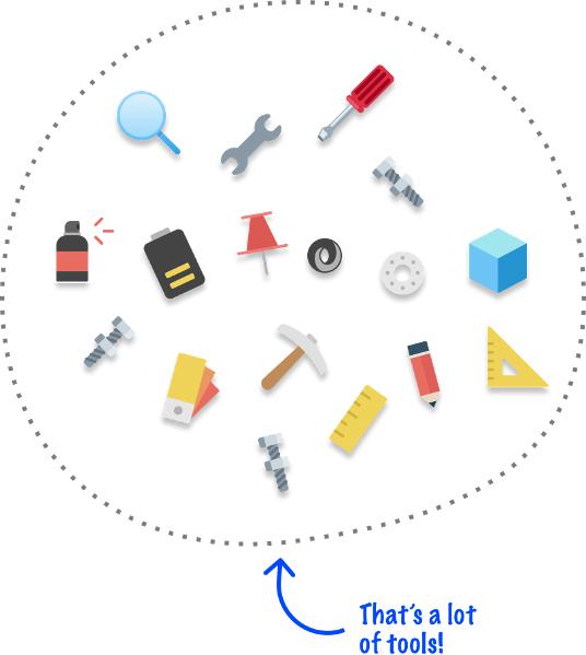
To better understand the importance of data structures, let’s look at an example. Here is the setup. We have a bunch of tools and related gadgets (Figure 1-1).
Figure 1-1 Tools,tools,tools
What we want to do is store these tools for easy access later. One solution is to simply throw all of the tools in a giant cardboard box and call it a day (Figure 1-2).
Figure 1-2 Tools,meetbox!
If we want to find a particular tool, we can rummage through our box to find what we are looking for. If what we are looking for happens to be buried deep in the bottom of our box, that’s cool. With enough rummaging (Figure 1-3)—and possibly shaking the box a few times—we will eventually succeed.
Figure 1-3 Arummager!
Now, there is a different approach we can take. Instead of throwing things into a box, we could store them in something that allows for better organization. We could store all of these tools in a toolbox (Figure 1-4).
Figure 1-4 Ourmetaphoricaltoolbox
A toolbox typically has many compartments to help us organize our tools. While it takes a bit of extra effort to store the items initially, all of this organization makes it easier for us to retrieve a tool later on. Instead of rummaging like a furry masked bandit through a pile of things, we can go directly to the appropriate pocket or compartment for the tool we need.
We have just seen two ways to solve our problem of storing our tools. If we had to summarize both approaches, it would look as follows:
Storing Tools in a Cardboard Box
Adding items is very fast. We just chuck it in there. Life is good.
Finding items is slow. If what we are looking for happens to be at the top, we can easily access it. If what we are looking for happens to be at the bottom, we’ll have to rummage through almost all of the items.
Removing items is slow as well. It has the same challenges as finding items. Things at the top can be removed easily. Things at the bottom may require some extra wiggling and untangling to safely get out.
Storing Tools in a Toolbox
Adding items to our box is slow. There are different compartments for different tools, so we need to ensure the right tool goes into the right location.
Finding items is fast. We go to the appropriate compartment and pick the tool from there.
Removing items is fast as well. Because the tools are organized in a good location, we can retrieve them without any fuss.
What we can see is that both our cardboard box and toolbox are good for some situations and bad for other situations. There is no universally right answer. If all we care about is storing our tools and never really looking at them again, stashing them in a cardboard box is the right choice. If we will be frequently accessing our tools, storing them in the toolbox is more appropriate.
Back to Data Structures
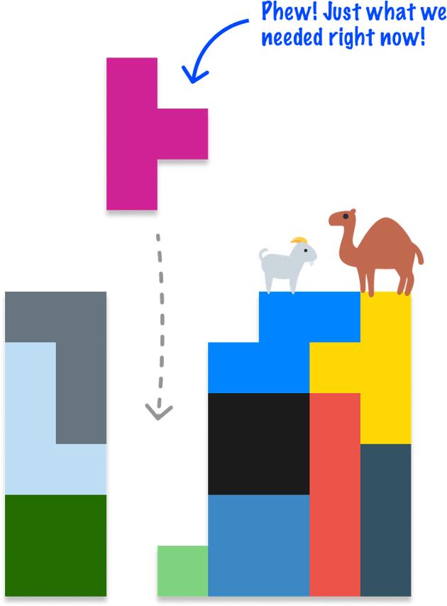
When it comes to programming and computers, deciding which data structure to use is similar to deciding whether to store our tools in a cardboard box or a toolbox. Every data structure we will encounter is good for some situations and bad for other situations (Figure 1-5).
Figure 1-5 Agoodfitinthiscase
Knowing which data structure to use and when is an important part of being an effective developer, and the data structures we need to deeply familiarize ourselves with are
Arrays
Linked lists
Stacks
Queues
Introduction to trees
Binary trees
Binary search trees
Heap data structure
Hashtable (aka hashmap or dictionary)
Trie (aka prefix tree)
Conclusion
Over the next many chapters, we’ll learn more about what each data structure is good at and, more important, what types of operations each is not very good at. By the end of it, you and I will have created a mental map connecting the right data structure to the right programming situation we are trying to address.
When analyzing the things our code does, we are interested in two things: time complexity and space complexity. Time complexity refers to how much time our code takes to run, and space complexity refers to how much additional memory our code requires.
In an ideal world, we want our code to run as fast as possible and take up as little memory as possible in doing so. The real world is a bit messier, so we need a way to consistently talk about how our code runs, how long it takes to run, and how much space it takes up. We need a way to compare whether one approach to solving a problem is more efficient than another. What we need is the Big-O (pronounced Big Oh) notation, and in the following sections, we’re going to learn all about it.
Onward!
It’s Example Time
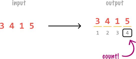
To help us better understand the Big-O notation, let us look at an example. We have some code, and our code takes a number as input and tells us how many digits are present. If our input number is 3415, the count of the number of digits is going to be 4 (Figure 21).
Figure 2-1 Countofdigitsinanumber
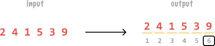
If our input number is 241,539, the number of digits will be 6 (Figure 2-2).
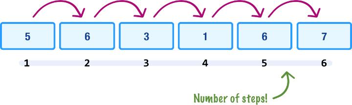
If we had to simplify the behavior, the amount of work we do to calculate the number of digits scales linearly with the size of our input number (Figure 2-3).
Figure 2-3 Thenumberofstepsscaleslinearly.
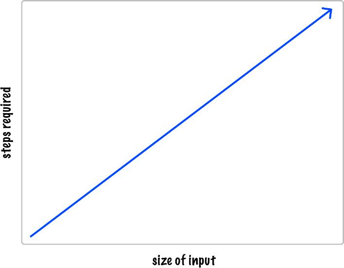
The larger the number we provide as the input, the more digits we have to count through to get the final answer. The important detail is that the number of steps in our calculation won’t grow abnormally large (or small) with each additional digit in our number. We can visualize this by plotting the sizeofourinputvs. the numberofsteps required to get the count (Figure 2-4).
What we see here is a visualization of linear growth! Linear growth is just one of many other rates of growth we will encounter.
Let’s say that we have some additional code that lets us know whether our input number is odd or even. The way we would calculate the oddness or evenness of a number is by just looking at the last number and doing a quick calculation (Figure 2-5).