Journal of Energy Storage
journal homepage: www.elsevier.com/locate/est
A novel graph-based framework for state of health prediction of lithium-ion battery
Xing-Yan Yao a, * , Guolin Chen a , Michael Pecht b , Bin Chen c
a Chongqing Engineering Laboratory for Detection Control and Integrated System, Chongqing Technology and Business University, Chongqing 400067, China
b Center for Advanced Life Cycle Engineering, University of Maryland, College Park, MD 20742, USA
c China Merchants Testing Vehicle Technology Research Institute Co., Ltd, Chongqing 400067, China
ARTICLE INFO
Keywords:
Lithium-ion battery (LIB)
State of health (SOH)
GraphSAGE
Graph neural network (GNN)
ABSTRACT


State of health (SOH) plays a vital role in lithium-ion batteries (LIBs) safety, reliability and lifetime. Health indicators (HIs) are a powerful approach to predict battery SOH. The existing methods for battery SOH prediction according to HIs only consider the temporal features of HIs. The spatial features of interdependence between HIs enrich predicational information especially for the limited data. This paper proposes a novel framework CLGraphSAGE to predict battery SOH based on graph neural network (GNN), which takes into both temporal and spatial features of HIs. Firstly, the Pearson's correlation coefficients between HIs and SOH are obtained to extract highly correlated HIs to build a graph. Subsequently, the temporal features are extracted by convolutional neural network (CNN) and long short-term memory neural network (LSTM). Finally, the spatial features are obtained by the graph sample aggregate (GraphSAGE) to propagate messages on a pre-defined graph structure, which uncovers the deep information among HIs. The effectiveness of the proposed approach in predicting battery SOH is verified by MIT, NASA datasets and the experimental datasets, and compared with CNN, LSTM and graph convolutional network and graph attention network. The results show that the root mean square error of the proposed approach CL-GraphSAGE can achieve 0.2 %, and the different datasets verify its feasibility.
1. Introduction
In response to extreme weather and environmental pollution, electric vehicles are widely used in the world. Lithium-ion batteries (LIBs) are a promising energy source for the electric vehicle due to their high energy, low self-discharge rate, and long storage life [1,2] Nevertheless, LIBs performance degrades with cycle increases. The battery failure can lead to serious or even safety accidents. Therefore, it is vital to monitor LIBs' state and master the battery health. The state of health (SOH) of the battery is a powerful tool to evaluate the battery current health condition and ensure battery safety and health management [3] SOH is a percentage of the maximum charge which can be released to the battery rated capacity. However, SOH is difficult to predict since it cannot be tested directly such as via terminal voltage. Moreover, the battery data collected in the real world is a limitation. It is a challenge to obtain
precise SOH due to the lack of data and indirectly measured parameters [4]
The methods for battery SOH prediction can be summarized as model-based and data-driven [5]. Model-based methods include electrochemical models [6,7], equivalent circuit models [8–11], and mathematical models [12–14] The electrochemical model-based method develops a model to describe the physical and chemical processes of a battery and then evaluate the influence of the aging process on the SOH. This method can be generally used for LIBs to obtain battery aging trajectories. However, the electrochemical model-based method requires lots of parameters, and SOH prediction performance is determined by the given parameters. In addition, the computational complexity is high. The equivalent circuit model is based on battery electrical characteristics combined with amounts of the dataset, and the lithium battery is equivalent to a circuit. Compared with the
Abbreviations: LIBs, lithium-ion batteries; SOH, state of health; HIs, health indicators; CL-GraphSAGE, the proposed method in this paper; GNN, graph neural network; GraphSAGE, graph sample aggregate; CNN, convolutional neural network; RNN, recurrent neural network; LSTM, long short-term memory neural network; CC, the current curve of the constant current; CV, the current curve of the constant voltage; G = (V , E ), graph G, E and V are the edge and node set; RMSE, root mean square error; MAPE, the average absolute percentage error; R2 , coefficient of determination.
* Corresponding author.
E-mail address: yaoxingyan-jsj@163.com (X.-Y. Yao).
https://doi.org/10.1016/j.est.2022.106437
Received 6 June 2022; Received in revised form 14 August 2022; Accepted 14 December 2022
Availableonline22December2022 2352-152X/©2022ElsevierLtd.Allrightsreserved.
electrochemical model, the computational complexity is less. Furthermore, mathematical models obtain the battery performance by large amounts of experimental data [4]. The SOH prediction is achieved via data analysis, fitting, trial and error, and statistical processing. In this method, the battery physical mechanism is a black box, and the SOH prediction is greatly affected by the experimental environment.
Data-driven methods achieve SOH prediction by utilizing battery signals (current, voltage, temperature, internal resistance, etc.) or health indicators (HIs) extracted from charging and discharging processes. This method does not know the battery complex internal mechanism. With the widespread application of artificial intelligence, machine learning has been widely used in lithium battery SOH prediction [15] Yang et al. [16] employed Gaussian process regression to predict SOH by four correlated HIs extracted from charging curves and analyzed the correlation between HIs and SOH. Song et al. [17] extracted features to describe the battery aging process and predict battery SOH. Yang et al. [18] extracted HIs from voltage and temperature during discharge, using a multiple kernel relevance vector machine that combined Gaussian with sigmoid function to improve the accuracy of SOH prediction. In addition, other machine learning methods such as random forest [19], Markov chain [20], Monte Carlo [21] and ARIMA [22] are also popular to use.
Although machine learning methods mentioned above achieved great success in processing nonlinear relationships, they are still can be improved to process historical data to predict battery SOH. Many researchers applied recurrent neural network (RNN) [23], gate recurrent unit (GRU) [24] and long-short term memory (LSTM) [25] to predict SOH. In addition, some researchers have used neural ordinary differential equations and recurrent neural networks for the analysis of batteries to predict SOH [26]. Kim et al. [27] used multiple features as the input of LSTM and changed the input sequence length to reflect the historical SOH. Cui et al. [28] proposed a dynamic spatial-temporal attention-based gated recurrent unit (DSTA-GRU) model, which considered both the time domain and space domain of features on SOH. The methods above mentioned typically used the historical data of HIs to establish the mapping between HIs and SOH. However, they ignore the potential interdependence between HIs and the interdependence between HIs on the prediction results either. Furthermore, it is urgent to deep mine hidden information from the limited battery data in the application.
The graph is a special type of data structure that describes the relationship between different entities. For the problem of multi-variate inputs, the graph uses variables as nodes, and the nodes are connected through their hidden dependency. In recent years, graph neural network (GNN) can effectively deal with complex graph structures and has attracted the attention of researchers in various fields [29–31] GNN relies on the relationships between nodes to capture information in the graph and optimizes the message-passing mechanism between graph nodes to get the dependence between different variables.
GNN has already used to prediction task right now. Yu et al. [32] used spatial-temporal graph convolutional networks to extract spatialtemporal features from the time series of the graph structure to predict traffic flow. Khodayar et al. [33] proposed a novel graph convolutional deep learning structure to predict short-term wind speed combined with LSTM. Vyas et al. [34] proposed a dynamic GNN to predict the soil moisture of multiple locations in a region over time. Wang et al. [35] construct a graph structure on a sensor network with Pearson Correlation Coefficients among sensors. In addition, they combined graph convolutional network and temporal convolutional networks to forecast the remaining useful life of the engine.
The data-driven approach can mine deep information in the limited data without much prior knowledge. The CNN is a powerful deep learning approach to extract local features. The LSTM has the advantage of long-term memory in sequence modeling to overcome the problems of gradient vanishing in the long sequence training. To deal with graph structure data, GNN is a kind of algorithm that uses neural networks to
learn graph structure data, extract and explore features in the graph structure data. GNN is a promising method to deal with time series prediction for data of spatial-temporal characteristics. The spatial characteristic is reflected by deep mining the interdependence between nodes of the features in the GNN, and the temporal characteristic can also be taken into considering the historical data according to the LSTM. As a kind of GNN, GraphSAGE can aggregate the information from nodes of the graph, and the message passing is used to learn features in the graph structure. Therefore, the fusion of CNN, LSTM and GraphSAGE can mine deep information from both the spatial features and temporal features of lithium-ion battery data to achieve SOH prediction. As far as we know, little research on SOH using GNN is demonstrated.
In this paper, a novel framework CL-GraphSAGE for battery SOH prediction is proposed. The HIs extracted from the charging and discharging process are converted into a graph structure. The combination of GNN and CNN-LSTM is employed for the node features and message passing information to obtain the spatial-temporal features of the graph.
The CNN-LSTM mines the potential temporal features of historical input of HIs data [36–38], which are used as node features of the graph structure. GraphSAGE is used to carry out message passing in the graph structure composed of HIs. Therefore, all the HIs can obtain complementary information from each other. The main contributions of this paper are as follows:
• A novel framework CL-GraphSAGE is proposed to predict lithium-ion battery SOH, which considers both the temporal and spatial features of HIs.
• The HIs highly correlated with SOH are extracted to form a spatialtemporal graph.
• The relationship between different HIs is deep mined and optimized to enrich the information to predict SOH.
• Graph neural network (GNN) is the first time to use for battery prediction problems.
The rest of the paper is organized as follows: Section 2 describes the lithium-ion battery datasets and feature extraction. Section 3 describes the CL-GraphSAGE SOH prediction method. Section 4 describes the results and discussions, followed by conclusions in Section 5
2. Datasets and feature extraction
This section describes two public lithium-ion battery datasets used to validate the method proposed in this paper. Different HIs are extracted for these two datasets.
2.1. Datasets
NASA datasets are used to verify the proposed method [39]. The B0005, B0006, and B0007 batteries are used. All battery charging and discharging processes are carried out at room temperature, with a nominal capacity of 2.0 Ah. During charging, the battery is first charged with a CC at 1.5 A until the voltage reaches 4.2 V; it is then charged with a CV until the current drops below 20 mA. During discharging, the battery is discharged with CC at 2A until cut-off voltage. Repeat the above steps until the battery reaches the end of its life (capacity loss 70 %). Fig. 1(a) shows the capacity curves of cycles.
The MIT lithium-ion battery dataset is currently the largest public dataset used for battery degradation research [40] The dataset consists of 124 commercial LIBs from A123. The nominal capacity and voltage are 1.1 Ah and 3.3 V, respectively. At 30 ◦ C, all batteries are charged with a multistep fast-charging strategy and then discharged with a CC process. The format of this strategy is “C1(Q1)-C2.” The battery is firstly charged by current C1 until the state of charge reaches S1, and then it is charged with current C2 until the state of charge reaches S2. The battery is charged from 80 % to 100 % SOC at 1C CC-CV. The cutoff voltage is 3.6 V. Subsequently, the battery is discharged at 4C CC, and the battery
life threshold is reduced to 80 % of the nominal capacity. The batteries A0001, A0002, and A0003 are employed in the experiments. Fig. 1(b) shows the capacity degradation of the specific cycle period.
2.2. Feature extraction
The HIs used for data-driven approaches depend on the dataset. Different HIs are extracted from NASA and MIT datasets. All the extracted HIs mentioned above are described in Table 1 The HIs involved in this article are divided into four categories, which are voltage-related, current-related, temperature-related, and time-related [41–43].
• Current-related HIs. The areas covered under the current curve of the CC process and the discharge process, the area covered under the current curve of the CV process, the CC-CV process, and the discharge process are as HIs. In addition, the maximum slope extracted from the CV process current curve is another HI.
Table 1
Four categories of HIs.
HI type No. HIs
Current-related
Voltage-related
Temperaturerelated
B1
B2
B3
B4
B5
B6
Area covered under current curves of the CC process
Area covered under current curves of CV process
Area covered under current curves of CC-CV process
Maximum slope of current curves in CV process
Area covered under current curves of discharge process
Area covered under voltage curves of CC process
B7 Area covered under voltage curves of CV process
B8 Area covered under voltage curves of discharge process
B9 Maximum slope of voltage curves in CC process
B10 Maximum temperature of charge and discharge cycles
B11 Minimum temperature of charge and discharge cycle
B12 Average temperature of charge and discharge cycle
B13 Area covered under temperature curves of charge and discharge cycle
B14
Area covered under temperature curves of the CC process
B15 Area covered under temperature curves of CV process
B16 Area covered under temperature curves of CC-CV process
Time-related B17
Discharge time
B18 Charging time
B19 CC stage period
B20 CV stage period
B21 CC stage end time
B22 Time to peak temperature during discharge
B23 The time ratio of the CC process and the entire charging process
B24 The time for voltages increases from 3.7 V to 4.2 V during the CC process
B25 Time for currents decreases from 1.5 A to 0.3 A during the CV process
B26 Time for voltages decreases from 3.7 V to 2.7 V during discharging
• Voltage-related HIs. The HIs extracted from the voltage curve are similar to the current-related HIs. The areas covered under the voltage curve of the CC process, CV process, and discharge process are HIs. The maximum slope extracted from the CC process voltage curve is also an HI.
• Temperature-related HIs. During the charging and discharging process, the temperature changes. The maximum temperature, minimum temperature, and average temperature are taken as HIs. The areas covered under the temperature curve of the CC process, CV process CC-CV process and the entire charge and discharge cycle are HIs.
• Time-related HIs. The HIs include CC charging time, CV charging time, charging time, and discharging time. In addition, the time for the temperature to reach the peak during the discharge process is also an HI.
The HIs extracted are multidimensional features. Different HIs have different degrees of correlation with SOH. If all HIs are used as input, it will affect the prediction accuracy and easily lead to overfitting. Therefore, given a threshold, the HIs with a lower correlation are eliminated, and the HIs with a higher correlation as the input of the model are kept. Pearson correlation coefficient [44] is used to evaluate the correlation between HIs and SOH.
The Pearson correlation coefficient calculates the linear correlation between HI and SOH in Eq. (1). Here, Xi and Yi are HI and SOH, respectively. μX and μY are the average values, respectively. The absolute value of Pearson's correlation coefficient is in the range of [0,1]. The larger the absolute value, the stronger the correlation. In this paper, the 6 most relevant HIs with large absolute values are selected as the final subset of HIs by the trials and errors of the experiments.
3. Methodology
This section describes in detail the proposed approach CLGraphSAGE for the battery SOH prediction in this paper. The components in CL-GraphSAGE are depicted in detail, and all steps of SOH prediction by CL-GraphSAGE are detailed descriptions.
3.1. CL-GraphSAGE
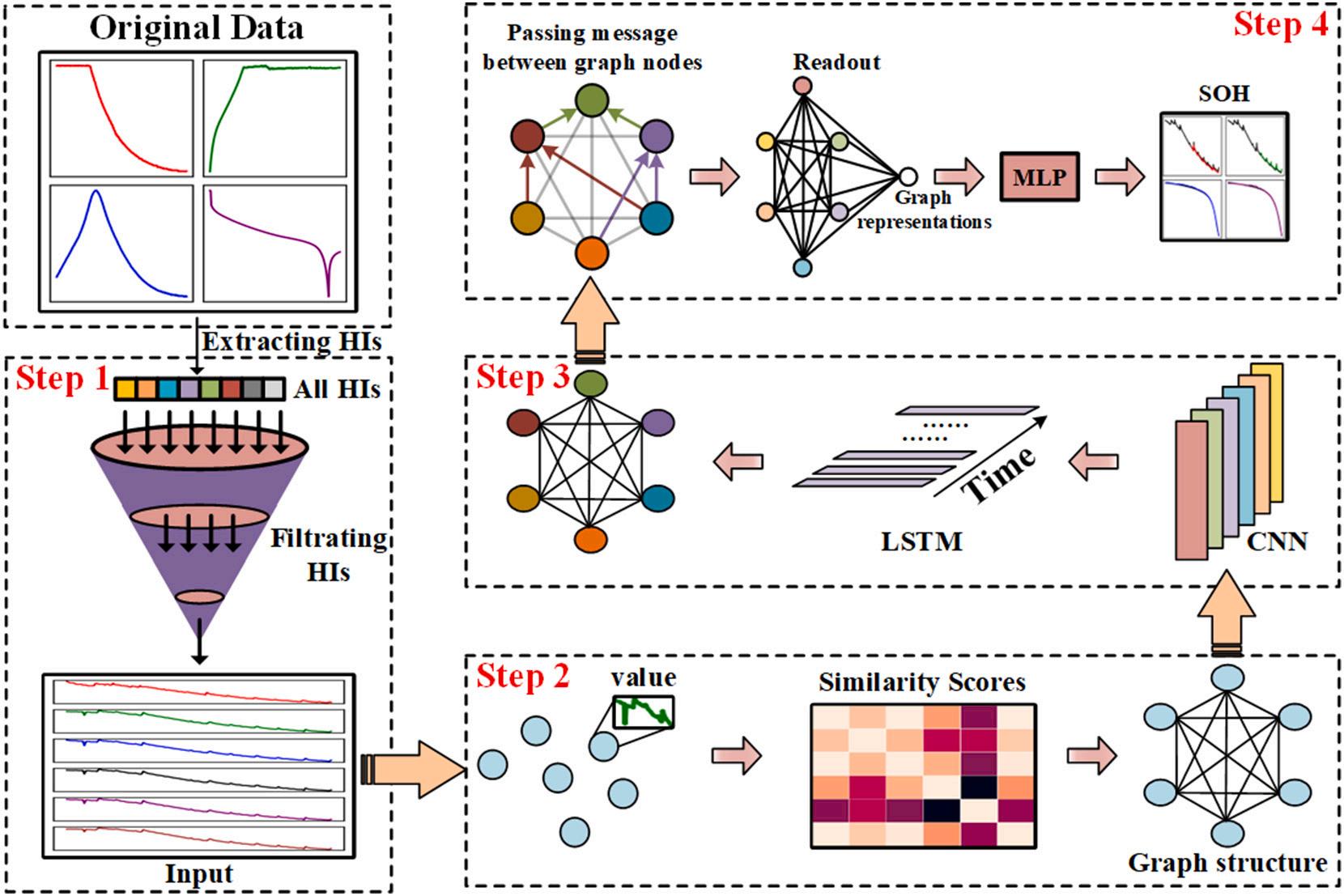
Fig. 2 shows the proposed CL-GraphSAGE for battery SOH prediction framework. The CL-GraphSAGE includes CNN, LSTM and GraphSAGE. The extracted HIs in Section 2 are used to build a graph structure. Then the HI's temporal features are extracted by CNN and LSTM, and the spatial features are obtained by GraphSAGE. Finally, the SOH is acquired by multilayer perceptron (MLP).
Fig. 1. Capacity degradation curves: (a) NASA datasets; (b) MIT datasets.
The details of CL-GraphSAGE are as follows:
Step 1: Extracting and filtrating HIs. The HIs are extracted from the original datasets. The HI subsets are derived from the Pearson correlation coefficient in Eq. (1).
Step 2: Building a graph structure. The input of GraphSAGE is a graph. The HI subset in Step 1 needs to be converted into a graph structure that consists of nodes and edges. Every filtrating HI is taken as one node of the graph. The similarity values between the HIs calculated by Eq. (2) are taken as edges of the graph. Therefore, the graph is represented by nodes set, and the HIs sequence data are the values of the nodes.
Step 3: Obtaining HIs temporal features. The HIs sequence data of each node is used as the input of the CNN-LSTM hybrid model. The HIs temporal features are the hidden state vector at the last moment of LSTM output.
Step 4: Updating node messages. The GraphSAGE is used to pass messages between graph nodes. The node message is updated by the center node, which receives all the connected node messages. All nodes are aggregated to obtain a global representation of the entire graph. Finally, SOH is predicted by MLP.
The pseudocode of the proposed CL-GraphSAGE is shown in Table 2
3.2. Graph structure of HIs
The determination of nodes and edges is the key to applying graph neural network to battery SOH prediction. In this paper, HIs are regarded as nodes in the graph, and HIs are connected as edges. Assuming a graph G = (V , E ), where E and V = {v1, v2, …, vn} are the edge and node set, respectively. Furthermore, the nodes consist of node sets and the corresponding node values. Here, the HIs subsets are the nodes of the graph, and the node values are obtained by the CNNLSTM hybrid model. |V| = n is the numbers of the HIs. For the i-th node, vi ∈ V with T-dimension is denoted by xi. X = {x1, x2, …, xn} ∈ Rn×T is the node feature vector.
For all the node vector V = {v1, v2, , vn}, the HIs are connected by
Table 2
Pseudocode of CL-GraphSAGE.
1: Input: The dataset , 2: Calculating similarity scores between HIs and building graph structure.
3: Training:
4: for in do:
5: ℎ ← ( ); 6: ℎ ← (ℎ);
7: ℎ ← ℎ (ℎ);
8: ℎ ← ℎ (ℎ); 9: ℎ ← (ℎ); 10: ← (ℎ);
11: Update model parameter.
12: end for 13: Output: The SOH of
the similarity values from the Eq. (2) [45] xi and xj are the sample sequence at i-th and j-th nodes, respectively. xi = xi /d is the average value of xi, and d is the number of elements of xi, and the range of i and j is [1, n].
Aij = (xi xi )T ( xj xj )
After defining the nodes and edges to build the graph, the task of SOH prediction is transformed to learn the mapping between HIs and SOH by the given SOH value at the time t. Specifically, the HIs at different timestamps are used as node data to generate temporal datasets for the graph, and the SOH at the time t is used for prediction in the graph.
3.3. Temporal feature of HIs
LSTM has been widely used in Lithium-ion battery SOH prediction. LSTM overcomes the problem of gradient vanishing and captures the long-term dependence of time series compared with RNN [46] LSTM
Fig. 2. CL-GraphSAGE framework for battery SOH prediction.
obtains the long-term dependence of time series data by using the storage unit to store useful information and the gating mechanism to discard useless information. LSTM structure includes input gates, forget gates, storage units, and output gates. The input gate saves the information, the forget gate obtains the forgetting information, the output gate represents the output information, and the storage unit keeps the historical information until the current moment.
CNN is a powerful tool to extract local hidden information of data by multi-layer convolution operations [47]. As shown in Fig. 3, CNN is used for extracting deep features from the historical information, which are the input of LSTM to mine temporal features of the sequence data. The feature extraction of every HI time series is separated from each other, and a one-dimensional CNN layer with one kernel of size 1 is used. HIs temporal features obtained by CNN and LSTM are used as the node features of the graph. The temporal features of every HI constitute the temporal feature matrix X of the graph.
3.4. GraphSAGE
For the SOH prediction, there are two keys to building the GNN model. One is to fuse the local information of nodes in the graph structure, and the other is to embed the updated nodes into vectors. In this paper, GraphSAGE aggregates the information of adjacent nodes to update nodes and obtains the interdependence between HIs. GraphSAGE is used to mine deep information between HIs of the edges in the graph. Therefore, each HI node contains all information of both HI itself and adjacent HIs from the k-layer GraphSAGE.
The input of GraphSAGE is the graph G = (V , E ) The node features X ∈ Rn×d , that are temporal features, are obtained in Section 3.3, where n is the number of HIs and d is the dimension of LSTM output. The similarity between HIs is calculated to obtain the connection between nodes of adjacency matrix A ∈ Rn×n in Section 3.2 The adjacency matrix A and the feature matrix X are used as the input of GraphSAGE.
Fig. 4 shows the aggregation process of GraphSAGE for the given graph. Fig. 4(b) displays the corresponding topological and node features by the given graph structure in Fig. 4(a). Taking the red node A in Fig. 4(a) as an example, GraphSAGE updates the information of the node A by fusing the neighborhoods' information. To update nodes at k-layer, the information of the adjacent nodes is first aggregated to hkN (v) by the aggregation function and then integrated and updated with the central node state hik 1 , which are shown in Eqs. (3)–(4) Then the aggregated embeddings hkN (i) are obtained by the neighborhood aggregation which is fused with the node information of the previous layer hik 1
N (v) = Aggregate({hk 1 j , ∀j ∈ N (i) } )
Here, hik is the state of the i-th node in the k-th message passing, and N (i) is the adjacent nodes set. In Eq. (4), the Aggregate function takes the place of the Mean aggregation function, and Eqs. (3)–(4) are combined and modified to obtain Eq. (5).
hk i = ReLU (W • Mean({hk 1 i } ∪ {hk 1 j , ∀j ∈ N (i) } ) ) (5)
After obtaining the final state of all nodes, the readout function is used to aggregate all node representations into a global representation of the graph [48]. The global expression is obtained by one-time aggregation of all inputs. Here, the Max function is to aggregate all nodes, and MLP outputs the final predicted value ̂ y t as shown in Eq. (6). The number of neurons in the output layer is 1 when the SOH value is at a certain moment. Huber loss [36] is used as the regression loss function. yt and ̂ y t are the true value and predicted value, respectively. δ is the hyperparameter in Eq. (7)
̂ y t = MLP( Readout( {hk i |i ∈ G}) ) (6)
3.5. Evaluation metrics
The experiments are carried out by PyTorch 3.8, Intel Core i710875H 2.30GHz CPU, and NVIDIA GEFORCE RTX 2060 GPU. Adam is the optimizer, the learning rate is 8e-4, the δ in the Huber loss objective function is set to 1, the number of training epochs is 1500, and the batch size is 16. Root mean square error (RMSE), average absolute percentage error (MAPE), and coefficient of determination (R2) are used to evaluate performances, which are as follows:
Fig. 3. Temporal feature matrix of HIs.
4. Experiments
This section validates the performances of CL-GraphSAGE to predict the SOH for different lithium-ion battery datasets. The three different datasets are employed to discuss the performance by comparing with different models.
4.1. Experiment for NASA dataset
According to HIs in Table 1 described in Section 2.2 and battery characteristics in Fig. 1(a). HIs are extracted from the NASA dataset. The correlation coefficient between HIs and SOH is obtained according to Eq. (2) shown in Table 3
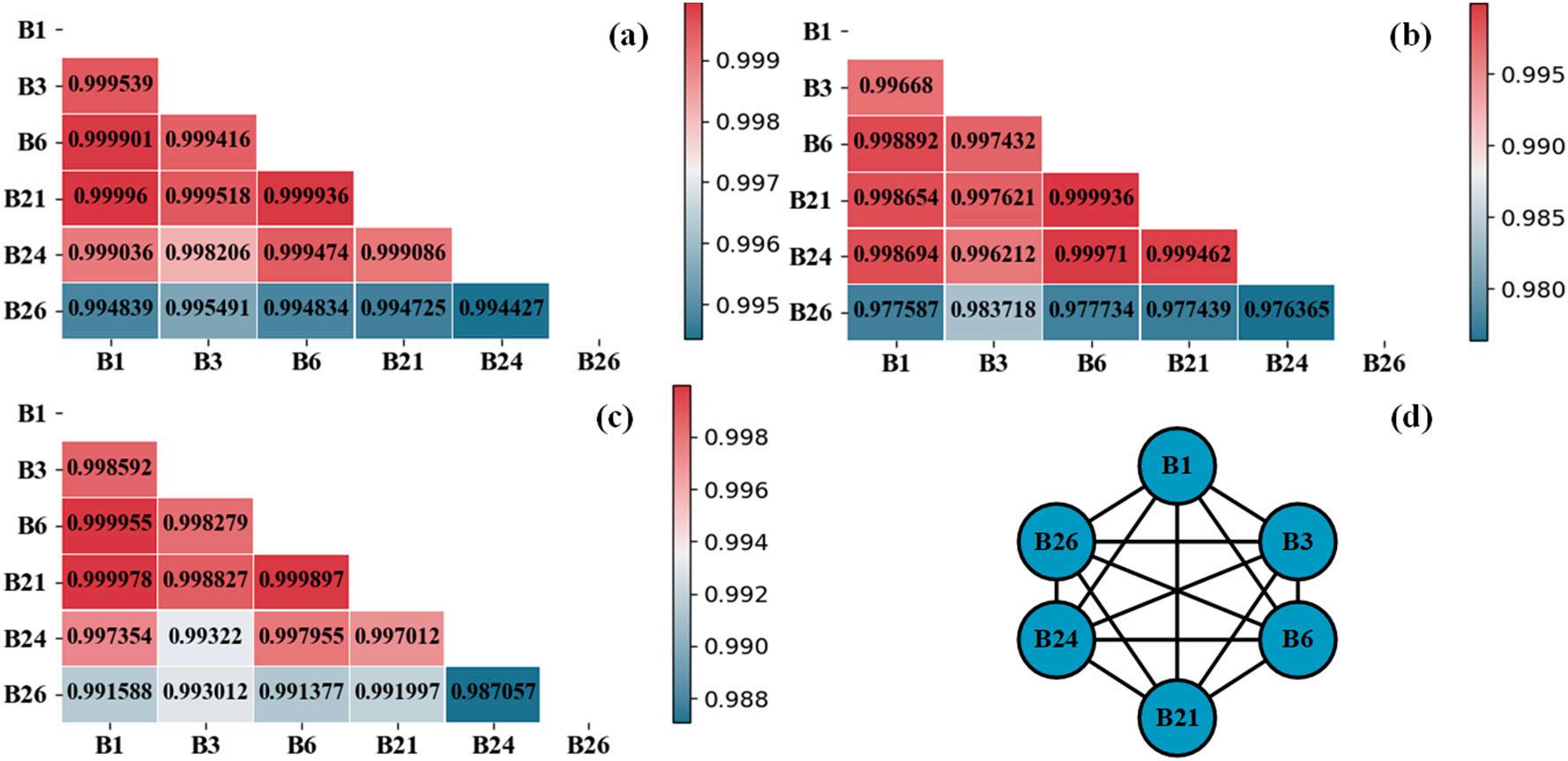
The first 6 high-correlation HIs (B1, B3, B6, B21, B24, and B26) are adopted as model inputs from Table 3. The similarity of HIs is calculated by Eq. (2). Fig. 5 shows the similarities between nodes. Two nodes with a similarity of 0.95 or more are connected into an edge. Taking B0005 as an example, as shown in Fig. 5(a), the similarities between HIs are all greater than 0.99. The nodes with a similarity of more than 0.95 are connected. Therefore, the six HIs are all connected as edges of the graph, and the graph structure is shown in Fig. 5(d). In Fig. 5(a)–(c), the similarity of HIs is greater than 0.95, and the graph structures are fully connected graphs.
The starting point is of great influence on the prediction results. The data before the starting point are used for training the model, and the remaining data are used for testing. Two kinds of training strategies are
Table 3
Descending order of correlation coefficient of HIs.
Sample Sort in descending order (from left to right, top to bottom)
carried out for the comparative experiments. The training data are chosen as the first 80 cycles and the first 100 cycles, respectively, and the corresponding remaining cycles are used as test data.
For the performance comparison, all the models are designed as multi-input and single-output. The 6 HIs selected above as the input of the models, and the battery SOH is the output of the models. The RNN is a classic approach to process sequence data and predicts battery SOH. RNN is a kind of neural network with sequence data as input. The output not only depends on the input at the current time but also is related to the input at the previous time. LSTM is a variant of RNN to improve the performance of RNN by overcoming the gradient vanishing when dealing with long-term memory. To mine the deep temporal features for the HIs sequence data, the CNN is combined with LSTM to predict SOH. In addition, GNN is used in the proposed CL-GraphSAGE to mine relevant information between HIs to obtain the spatial features of HIs. Through comparative verification, GNN has improved the SOH prediction accuracy. The performance of three models RNN, LSTM, and CNNLSTM are compared with CL-GraphSAGE.
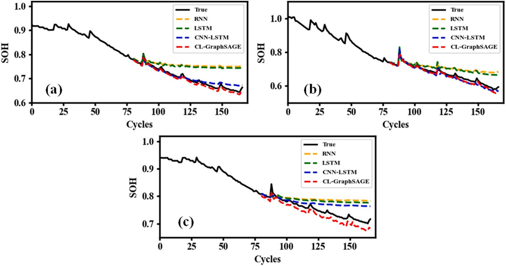
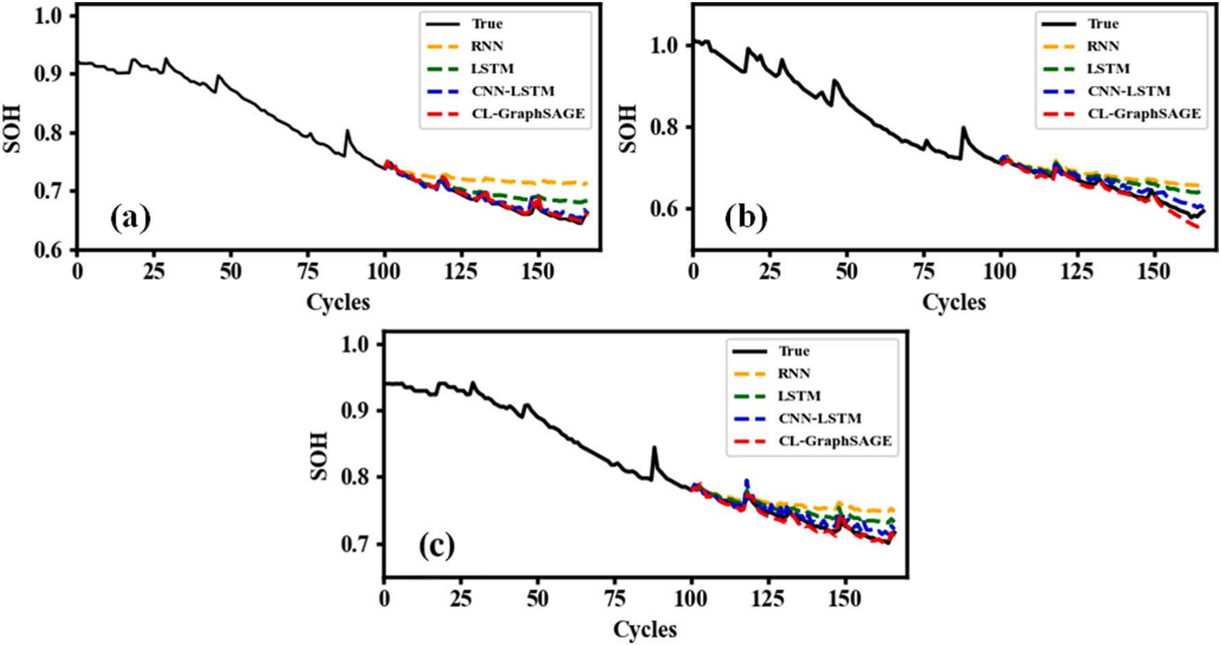
Fig. 6 shows the results starting at 81of the four models in B0005, B0006, and B0007. Table 4 shows the performance evaluation of the four models from the different starting points. The RMSE of RNN and LSTM are both larger than 0.04, and the MAPE is larger than 4.5. The RMSE of CNN-LSTM and CL-GraphSAGE are both less than 0.035, and the MAPE are both less than 3.5. In some experiments, R2 of LSTM and RNN is even less than 0, which indicates that LSTM and RNN have poor adaptability and poor predictive ability in these cases. Therefore, the performance of RNN and LSTM in these three batteries is worse than that of CNN-LSTM and CL-GraphSAGE. As cycle numbers increase, the predicted result tends to be a straight line and cannot reflect the nonlinear capacity degradation trend. However, in Fig. 6(c), the predicted result of CNN-LSTM is consistent with that of RNN and LSTM, which is quite different from the true SOH.
The bold in the table are the selected HIs which is the input of the model in this case study.
Fig. 4. Aggregation process of GraphSAGE: (a) the given graph; (b) aggregated embedding.
However, the predicted results by CL-GraphSAGE can still capture the tendency of capacity degradation, which indicates the proposed CLGraphSAGE is feasibility to the battery SOH prediction. The RMSE and MAPE of CL-GraphSAGE are the lowest among the three experiments. In battery B0007, the RMSE and MAPE are 0.019028 and 2.383225, respectively, which are much lower than CNN-LSTM. The prediction results of CL-GraphSAGE show good performance. Compared with the other three models in Table 4, CL-GraphSAGE makes full use of the spatio-temporal features of HIs. CL-GraphSAGE can mine the relationship information between HIs and is better for SOH prediction.
Fig. 7 shows results starting at 101 of the four models in B0005, B0006, and B0007. According to Fig. 7, the prediction results of the three models are closer to the actual capacity degradation trend by using more training data. The RMSE and MAPE of RNN and LSTM are larger than those of CNN-LSTM and CL-GraphSAGE.
Table 4 shows the prediction errors of the four models at different starting points for different lithium-ion battery samples. In Table 4, both
RMSE and MAPE of CL-GraphSAGE are the lowest compared with CNNLSTM, which shows good prediction performance. Moreover, CLGraphSAGE predicts accurately when the starting point is 101 compared with the starting point at 81. The results show that regardless of whether the prediction starting point is 81 or 101, CL-GraphSAGE is the best choice.
4.2. Experiment of MIT dataset
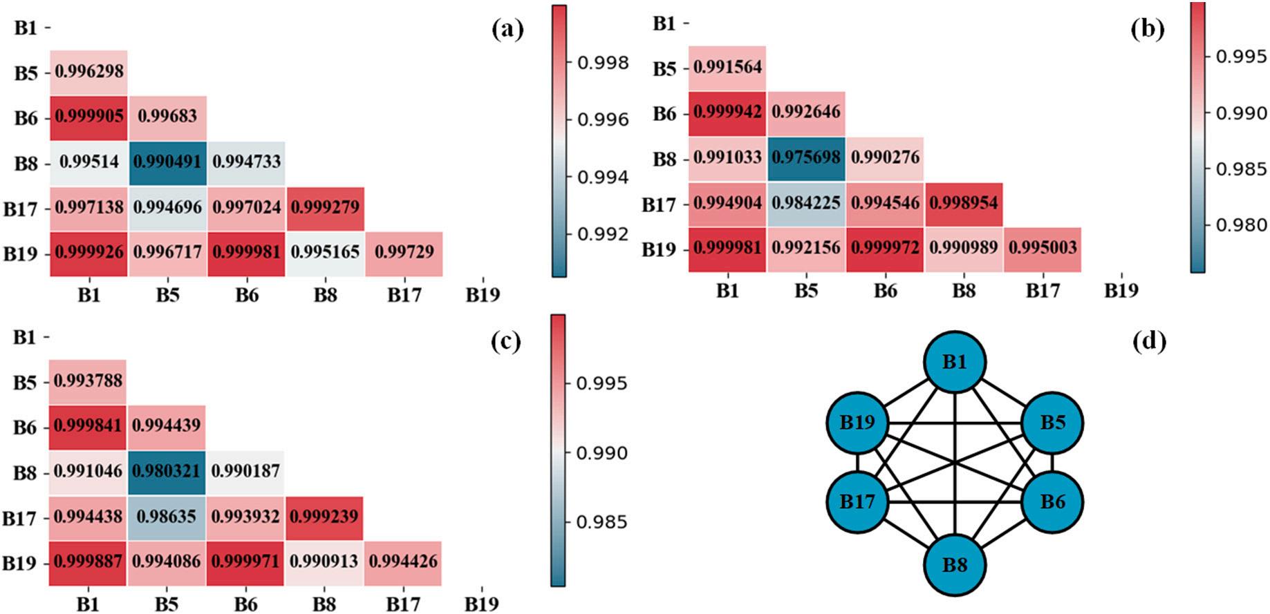
According to HIs in Table 1 described in Section 2.2 and battery capacity in Fig. 1(b), all HIs extracted from the MIT dataset and the correlation coefficient between HIs and SOH are obtained according to Eq. (2) are shown in Table 5 The first six high-correlation HIs (B1, B5, B6, B8, B17, and B19) are selected as model inputs.
The method to construct the nodes and edges of the graph is the same as in Section 4.1. Fig. 8 shows the similarities between nodes. The similarity values are displayed in Fig. 8(a)–(c). The two nodes are
Fig. 5. Node similarity and graph structure: (a) B0005; (b) B0006; (c) B0007; (d) graph of B0005 HIs.
Fig. 6. Prediction results at starting point of 81: (a) B0005; (b) B0006; (c) B0007.
Table 4
Predicting errors at different starting points by different models. Sample
0.720849 0.951118
GraphSAGE 0.005808 0.625176 0.958309
B0006 RNN 81 0.046791 5.955632 0.131731 LSTM 0.041631 5.451267 0.312677
CNN-LSTM 0.013927 1.802672 0.923077 CLGraphSAGE 0.011475 1.470694 0.947783
101 0.036882 4.796715 0.130402
0.027935 3.581093 0.501154
0.013923 1.884062 0.876073
GraphSAGE 0.010859 1.331990 0.924613 B0007 RNN 81 0.045730 5.199274 0.879691
0.041061 4.671529 0.515507 CNN-LSTM 0.031836 3.398467 0.088939
GraphSAGE 0.019028 2.383225 0.674550
101 0.025090 2.852394 0.096398
0.015771 1.766805 0.566800
0.008994 0.956124 0.859108
GraphSAGE 0.005314 0.606468 0.950810
connected when the similarity value is more than 0.95. All the graph structures are fully connected graphs. Fig. 8(d) shows the graph structures of the battery B0005 HIs.
Compared with the NASA dataset, the MIT dataset has more cycles and a larger amount of data. Different training method is employed in the MIT dataset. A0001 is used for training, and A0002 and A0003 are used for testing.
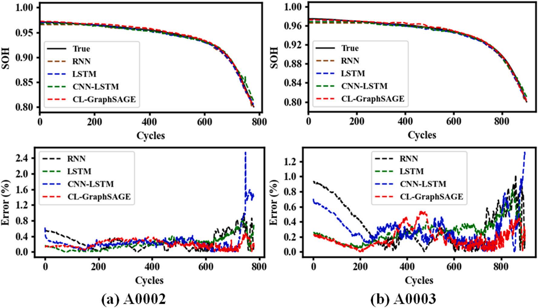
Fig. 9 shows the prediction results and errors. Table 6 shows the performance evaluation of the four models. Compared with the other three models, CL-GraphSAGE obtains the best prediction performance,
which is the lowest RMSE, MAPE with the highest R2
Experiment results show that the proposed method is better than the comparison model in terms of SOH prediction. Compared with the other three models, CL-GraphSAGE can obtain not only the temporal features of HIs using CNN and LSTM but also the spatial features between HIs. Therefore, CL-GraphSAGE can make full use of the interrelationships between different HIs to deep mine more useful potential features. The fluctuation range of the prediction error of CL-GraphSAGE is smaller for SOH prediction compared with the other three models.
4.3. Experiment of laboratory dataset
In this section, the lithium-ion battery dataset carried out in the laboratory is used to validate the feasibility of CL-GraphSAGE. The experiments are carried out in China Merchants Testing Vehicle Technology Research Institute Co., Ltd. The BAT-NEEFLCT-05500 from NEBULA Co., Ltd. is used to cycle the batteries. The data is collected by Agilent 34901A.
The batteries go through 4 steps in each cycle: 1) Discharging CC at 58A until the voltage drop to 2.5 V. 2) The battery is rest for 1800 s. 3) Charging CC at 38.86 A until the voltage increases to 4.25 V, then CV at 4.25 V until the current drop to 2.9A. 4) Resting 1800 s.
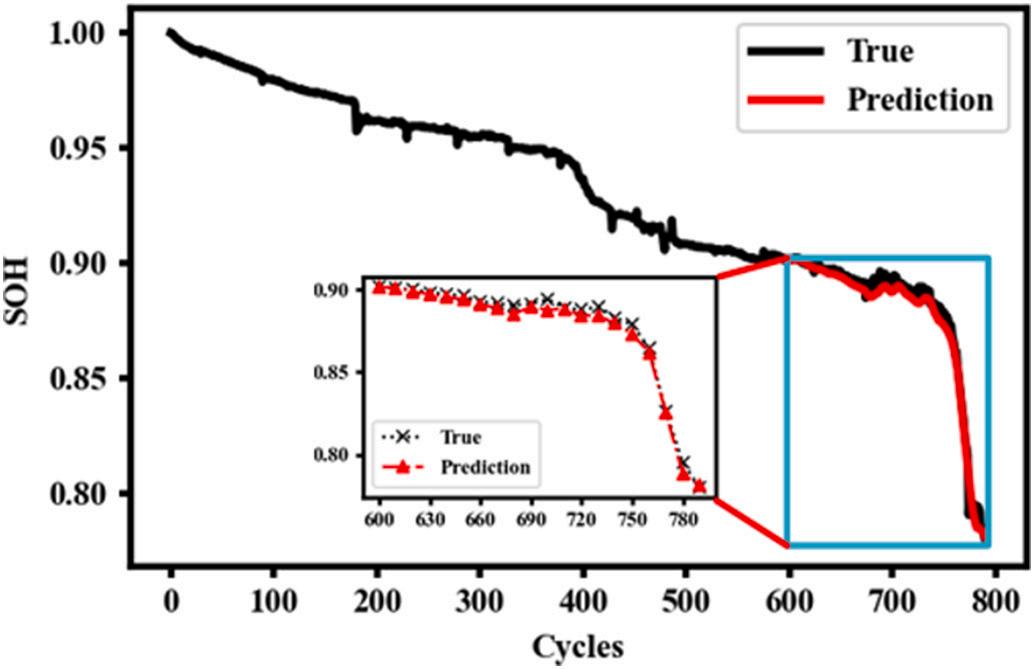
Five strongly correlated HIs (B3, B5, B8, B17, B26) are taken as model input from the charge-discharge curves as CL-GraphSAGE input by using HIs extracted in Section 2.2 The predicted results are shown in Fig. 10 Fig. 10 shows that the CL-GraphSAGE well captures the degradation of LIBs. The RMSE and R2 are 0.003688 and 0.986188, respectively. Both RMSE and R2 verify the effectiveness of CL-GraphSAGE.
4.4. Experiment of different graph models
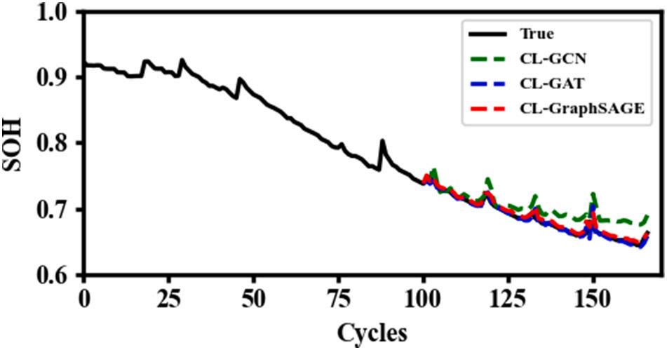
Instead of using GraphSAGE in the NASA dataset, combined with CNN and LSTM, the graph convolutional network (GCN) and graph attention network (GAT) which are CL-GCN and CL-GAT used to compare with the CL-GraphSAGE. The results are shown in Fig. 11 and Table 7. The results are similar to that of CL-GAT and CL-GraphSAGE. However, the running time of CL-GCN, CL-GAT, and CL-GraphSAGE are 169.21 s, 462.63 s, and 110.38 s, respectively. The execution time of CL-GAT is more than four times that of CL-GraphSAGE. In terms of time cost and prediction accuracy, CL-GraphSAGE is the best of the three GCNs proposed in this paper to obtain the spatial features of HIs.
Fig. 7. Prediction results at starting point of 101: (a) B0005; (b) B0006; (c) B0007.
Table 5
Descending order of correlation coefficient for HIs.
Sample Sort in descending order (from left to right, top to bottom)
The bold in the table are the selected HIs which is the input of the model in this case.
Fig. 8. Node similarity and graph structure: (a) A0001; (b) A0002; (c) A0003; (d) graph of A0001 HIs.
Fig. 9. SOH prediction results: (a) A0002; (b) A0003.
Table 6
Performance evaluation with different models.
Sample
A0002 RNN 0.003048 0.264716 0.993135 LSTM 0.002468 0.215389 0.995500
CNN-LSTM 0.003383 0.266529 0.991545
CL-GraphSAGE 0.002070 0.197313 0.996834
A0003 RNN 0.004226 0.353931 0.987291
LSTM 0.002776 0.266655 0.994514
CNN-LSTM 0.003361 0.304047 0.991960
CL-GraphSAGE 0.002114 0.184998 0.996818
Fig. 10. Prediction results of CL-GraphSAGE.
Fig. 11. Results of the three GNN models.
Table 7
Errors of the three GNN models.
Method RMSE MAPE R2
CL-GCN 0.020253 2.504092 0.493080
CL-GAT 0.006454 0.505244 0.948513
CL-GraphSAGE 0.005808 0.625176 0.958309
5. Conclusions
The current lithium-ion battery SOH predicted methods by health indicators only take time features into account and ignore the relationship between different features especially for the limited data in the application. In this paper, a novel GNN-based framework is proposed for SOH prediction, which considers both the temporal features and the spatial features of HIs for the limited data. The validation and feasibility of the proposed CL-GraphSAGE are proved by public battery datasets and laboratory experiments. The results show that the CL-GraphSAGE reached minimum error and predicts more accurately and precisely
compared with RNN, LSTM, and CNN-LSTM.
It is understood that there is little research on GNN in LIBs. This work opens a new door for using GNNs to process various structural or unstructured data of batteries. Naturally, there are some limitations to the method. The future work includes: (1) The correlated HIs extracted based on partial charge-discharge curves will be developed in the future. (2) The edges connected are fixed weight by calculating the Pearson correlation coefficient in the proposed approach, which are all fully connected in the graph. Hence, the weight of the edges can be designed to update automatically to determine which edge to connect adaptively. (3) GNN can also be applied to other aspects of batteries, such as remaining life prediction, thermal runaway warning, and fault diagnosis.
CRediT authorship contribution statement
Xing-Yan Yao: Conception, Methodology, Validation, Formal analysis, Investigation, Writing - Original Draft, Writing - Review & Editing, Visualization, Guolin Chen: Conceptualization, Methodology, Software, Validation, Writing, Bin Chen: providing dataset, Michael Pecht: Review, Supervision.
Declaration of competing interest
The authors declare that they have no known competing financial interests or personal relationships that could have appeared to influence the work reported in this paper.
Data availability
Data will be made available on request.
Acknowledgments
This work is partially supported by the National Natural Science Foundation of China (51605061); Science and Technology Research Project of Chongqing Municipal Education Commission (KJQN201900808); Natural Science Foundation of Chongqing, China (cstc2020jcyj-msxmX0736); Innovation and Entrepreneurship Demonstration Team of Chongqing Talent Plan (CQYC201903246); Startup Project of Doctor Scientific Research (2016-56-04) and Open Grant of Chongqing Engineering Laboratory for Detection Control and Integrated System (KFJJ2021018). The valuable comments and suggestions from the anonymous reviewer are appreciated. Thanks for NASA and MIT provide the battery datasets.
References
[1] X. Hu, F. Feng, K. Liu, et al., State estimation for advanced battery management: key challenges and future trends[J], Renew. Sust. Energ. Rev. 114 (2019), 109334
[2] P.M. Attia, A. Grover, N. Jin, et al., Closed-loop optimization of fast-charging protocols for batteries with machine learning[J], Nature 578 (7795) (2020) 397–402
[3] X. Tang, C. Zou, K. Yao, et al., A fast estimation algorithm for lithium-ion battery state of health[J], J. Power Sources 396 (2018) 453–458
[4] H. Tian, P. Qin, K. Li, et al., A review of the state of health for lithium-ion batteries: research status and suggestions[J], J. Clean. Prod. 261 (2020), 120813
[5] R. Xiong, L. Li, J. Tian, Towards a smarter battery management system: a critical review on battery state of health monitoring methods[J], J. Power Sources 405 (2018) 18–29
[6] J. Li, K. Adewuyi, N. Lotfi, et al., A single particle model with chemical/mechanical degradation physics for lithium ion battery state of health (SOH) estimation[J], Appl. Energy 212 (2018) 1178–1190.
[7] G.K. Prasad, C.D. Rahn, Model based identification of aging parameters in lithium ion batteries[J], J. Power Sources 232 (2013) 79–85
[8] X. Hu, H. Yuan, C. Zou, et al., Co-estimation of state of charge and state of health for lithium-ion batteries based on fractional-order calculus[J], IEEE Trans. Veh. Technol. 67 (11) (2018) 10319–10329
[9] Z. Guo, X. Qiu, G. Hou, et al., State of health estimation for lithium ion batteries based on charging curves[J], J. Power Sources 249 (2014) 457–462
[10] J. Kim, B.H. Cho, State-of-charge estimation and state-of-health prediction of a liion degraded battery based on an EKF combined with a per-unit system[J], IEEE Trans. Veh. Technol. 60 (9) (2011) 4249–4260
[11] J. Yang, B. Xia, W. Huang, et al., Online state-of-health estimation for lithium-ion batteries using constant-voltage charging current analysis[J], Appl. Energy 212 (2018) 1589–1600
[12] X. Feng, J. Li, M. Ouyang, et al., Using probability density function to evaluate the state of health of lithium-ion batteries[J], J. Power Sources 232 (2013) 209–218
[13] A. Guha, A. Patra, State of health estimation of lithium-ion batteries using capacity fade and internal resistance growth models[J], IEEE Trans. Transp. Electrification 4 (1) (2017) 135–146
[14] P. Singh, C. Chen, C.M. Tan, et al., Semi-empirical capacity fading model for SoH estimation of li-ion batteries[J], Appl. Sci. 9 (15) (2019) 3012
[15] Z. Deng, X. Hu, P. Li, et al., Data-driven battery state of health estimation based on random partial charging data[J], IEEE Trans. Power Electron. 37 (5) (2021) 5021–5031
[16] D. Yang, X. Zhang, R. Pan, et al., A novel gaussian process regression model for state-of-health estimation of lithium-ion battery using charging curve[J], J. Power Sources 384 (2018) 387–395
[17] S. Song, C. Fei, H. Xia, Lithium-ion battery SOH estimation based on XGBoost algorithm with accuracy correction[J], Energies 13 (4) (2020) 812
[18] Y. Yang, J. Wen, Y. Shi, et al., State of health prediction of lithium-ion batteries based on the discharge voltage and temperature[J], Electronics 10 (12) (2021) 1497
[19] K.S.R. Mawonou, A. Eddahech, D. Dumur, et al., State-of-health estimators coupled to a random forest approach for lithium-ion battery aging factor ranking[J], J. Power Sources 484 (2021), 229154
[20] R. Xiong, J. Cao, Q. Yu, Reinforcement learning-based real-time power management for hybrid energy storage system in the plug-in hybrid electric vehicle [J], Appl. Energy 211 (2018) 538–548
[21] R. Xiong, Y. Zhang, J. Wang, et al., Lithium-ion battery health prognosis based on a real battery management system used in electric vehicles[J], IEEE Trans. Veh. Technol. 68 (5) (2018) 4110–4121
[22] Z. Yun, W. Qin, W. Shi, et al., State-of-health prediction for lithium-ion batteries based on a novel hybrid approach[J], Energies 13 (18) (2020) 4858
[23] P. Venugopal, State-of-health estimation of li-ion batteries in electric vehicle using IndRNN under variable load condition[J], Energies 12 (22) (2019) 4338
[24] Y. Fan, F. Xiao, C. Li, et al., A novel deep learning framework for state of health estimation of lithium-ion battery[J], J. Energy Storage 32 (2020), 101741.
[25] Z. Deng, X. Lin, J. Cai, et al., Battery health estimation with degradation pattern recognition and transfer learning[J], J. Power Sources 525 (2022), 231027
[26] S. Pepe, J. Liu, E. Quattrocchi, et al., Neural ordinary differential equations and recurrent neural networks for predicting the state of health of batteries[J], J. Energy Storage 50 (2022), 104209
[27] S.J. Kim, S.H. Kim, H.M. Lee, State of health estimation of Li-ion batteries using multi-input LSTM with optimal sequence length[C], in: 2020 IEEE 29th International Symposium on Industrial Electronics (ISIE), IEEE, 2020, pp. 1336–1341
[28] S. Cui, I. Joe, A dynamic spatial-temporal attention-based GRU model with healthy features for state-of-health estimation of lithium-ion batteries[J], IEEE Access 9 (2021) 27374–27388
[29] Z. Wu, S. Pan, G. Long, Connecting the dots: multivariate time series forecasting with graph neural networks[C], in: Proceedings of the 26th ACM SIGKDD International Conference on Knowledge Discovery & Data Mining, 2020, pp. 753–763
[30] H. Xu, Y. Huang, Z. Duan, Multivariate Time Series Forecasting With Transfer Entropy Graph[J], arXiv preprint arXiv:2005.01185, 2020
[31] Y. Wang, Z. Duan, Y. Huang, et al., MTHetGNN: a heterogeneous graph embedding framework for multivariate time series forecasting[J], Pattern Recogn. Lett. 153 (2022) 151–158
[32] B. Yu, H. Yin, Z. Zhu, Spatio-temporal Graph Convolutional Networks: A Deep Learning Framework for Traffic Forecasting[J], arXiv preprint arXiv:1709.04875, 2017
[33] M. Khodayar, J. Wang, Spatio-temporal graph deep neural network for short-term wind speed forecasting[J], IEEE Trans. Sustain. Energy 10 (2) (2018) 670–681.
[34] A. Vyas, S. Bandyopadhyay, Semi-supervised Soil Moisture Prediction Through Graph Neural Networks[J], arXiv preprint arXiv:2012.03506, 2020
[35] M. Wang, Y. Li, Y. Zhang, et al., Spatio-temporal graph convolutional neural network for remaining useful life estimation of aircraft engines[J], Aerosp. Syst. 4 (1) (2021) 29–36
[36] B. Zraibi, C. Okar, H. Chaoui, et al., Remaining useful life assessment for lithiumion batteries using CNN-LSTM-DNN hybrid method[J], IEEE Trans. Veh. Technol. 70 (5) (2021) 4252–4261
[37] X. Song, F. Yang, D. Wang, et al., Combined CNN-LSTM network for state-of-charge estimation of lithium-ion batteries[J], IEEE Access 7 (2019) 88894–88902
[38] G. Zou, Z. Yan, C. Zhang, Transfer learning with CNN-LSTM model for capacity prediction of lithium-ion batteries under small sample[C], in: Journal of Physics: Conference Series 2258(1), IOP Publishing, 2022, p. 012042
[39] B. Sahaand, K. Goebel, Battery Data Set, NASA Ames Prognostics Data Repository [J], NASA Ames Research Center, 2007
[40] K.A. Severson, P.M. Attia, N. Jin, et al., Data-driven prediction of battery cycle life before capacity degradation[J], Nat. Energy 4 (5) (2019) 383–391
[41] Z. Fei, F. Yang, K.L. Tsui, et al., Early prediction of battery lifetime via a machine learning based framework[J], Energy 225 (2021), 120205
[42] P. Guo, Z. Cheng, L. Yang, A data-driven remaining capacity estimation approach for lithium-ion batteries based on charging health feature extraction[J], J. Power Sources 412 (2019) 442–450
[43] Y. Li, D.I. Stroe, Y. Cheng, et al., On the feature selection for battery state of health estimation based on charging–discharging profiles[J], J. Energy Storage 33 (2021), 102122.
[44] G. Chandrashekar, F. Sahin, A survey on feature selection methods[J], Comput. Electr. Eng. 40 (1) (2014) 16–28
[45] L. Qiao, L. Zhang, S. Chen, et al., Data-driven graph construction and graph learning: a review[J], Neurocomputing 312 (2018) 336–351
[46] J. Niu, C. Liu, L. Zhang, Remaining useful life prediction of machining tools by 1DCNN LSTM network[C], in: 2019 IEEE Symposium Series on Computational Intelligence (SSCI), IEEE, 2019, pp. 1056–1063
[47] T.Y. Kim, S.B. Cho, Predicting residential energy consumption using CNN-LSTM neural networks[J], Energy 182 (2019) 72–81
[48] J. Gilmer, S.S. Schoenholz, P.F. Riley, Neural message passing for quantum chemistry[C], in: International Conference on Machine Learning. PMLR, 2017, pp. 1263–1272
Other documents randomly have different content
coup de canon retentit sur la plaine blanche de l’Océan. Une sueur froide coula sur le front du jeune officier. Il était sans épée. Il comprenait que ses soldats avaient péri et que les Anglais allaient débarquer. Il se vit déshonoré s’il vivait, il se vit traduit devant un conseil de guerre; alors il mesura des yeux la profondeur de la vallée, et s’y élançait au moment où la main de Clara saisit la sienne.
—Fuyez! dit-elle, mes frères me suivent pour vous tuer. Au bas du rocher, par là, vous trouverez l’andaloux de Juanito. Allez!
Elle le poussa, le jeune homme stupéfait la regarda pendant un moment; mais, obéissant bientôt à l’instinct de conservation qui n’abandonne jamais l’homme, même le plus fort, il s’élança dans le parc en prenant la direction indiquée, et courut à travers des rochers que les chèvres avaient seules pratiqués jusqu’alors. Il entendit Clara crier à ses frères de le poursuivre; il entendit les pas de ses assassins; il entendit siffler à ses oreilles les balles de plusieurs décharges; mais il atteignit la vallée, trouva le cheval, monta dessus et disparut avec la rapidité de l’éclair.
En peu d’heures le jeune officier parvint au quartier du général G...t...r, qu’il trouva dînant avec son état-major.
—Je vous apporte ma tête! s’écria le chef de bataillon en apparaissant pâle et défait.
Il s’assit, et raconta l’horrible aventure. Un silence effrayant accueillit son récit.
—Je vous trouve plus malheureux que criminel, répondit enfin le terrible général. Vous n’êtes pas comptable du forfait des Espagnols; et à moins que le maréchal n’en décide autrement, je vous absous.
Ces paroles ne donnèrent qu’une bien faible consolation au malheureux officier.
—Quand l’empereur saura cela! s’écria-t-il.
—Il voudra vous faire fusiller, dit le général, mais nous verrons. Enfin, ne parlons plus de ceci, ajouta-t-il d’un ton sévère, que pour
en tirer une vengeance qui imprime une terreur salutaire à ce pays où l’on fait la guerre à la façon des Sauvages.
Une heure après, un régiment entier, un détachement de cavalerie et un convoi d’artillerie étaient en route. Le général et Victor marchaient à la tête de cette colonne. Les soldats, instruits du massacre de leurs camarades, étaient possédés d’une fureur sans exemple. La distance qui séparait la ville de Menda du quartier général fut franchie avec une rapidité miraculeuse. Sur la route, le général trouva des villages entiers sous les armes. Chacune de ces misérables bourgades fut cernée et leurs habitants décimés.
Par une de ces fatalités inexplicables, les vaisseaux anglais étaient restés en panne sans avancer; mais on sut plus tard que ces vaisseaux ne portaient que de l’artillerie et qu’ils avaient mieux marché que le reste des transports. Ainsi la ville de Menda, privée des défenseurs qu’elle attendait, et que l’apparition des voiles anglaises semblait lui promettre, fut entourée par les troupes françaises presque sans coup férir. Les habitants, saisis de terreur, offrirent de se rendre à discrétion. Par un de ces dévouements qui n’ont pas été rares dans la Péninsule, les assassins des Français, prévoyant, d’après la cruauté connue du général, que Menda serait peut-être livrée aux flammes et la population entière passée au fil de l’épée, proposèrent de se dénoncer eux-mêmes au général. Il accepta cette offre, en y mettant pour condition que les habitants du château, depuis le dernier valet jusqu’au marquis, seraient mis entre ses mains. Cette capitulation consentie, le général promit de faire grâce au reste de la population et d’empêcher ses soldats de piller la ville ou d’y mettre le feu. Une contribution énorme fut frappée, et les plus riches habitants se constituèrent prisonniers pour en garantir le paiement, qui devait être effectué dans les vingt-quatre heures.
Le général prit toutes les précautions nécessaires à la sûreté de ses troupes, pourvut à la défense du pays, et refusa de loger ses soldats dans les maisons. Après les avoir fait camper, il monta au château et s’en empara militairement. Les membres de la famille de Léganès et les domestiques furent soigneusement gardés à vue, garrottés, et enfermés dans la salle où le bal avait eu lieu. Des fenêtres de cette pièce on pouvait facilement embrasser la terrasse
qui dominait la ville. L’état-major s’établit dans une galerie voisine, où le général tint d’abord conseil sur les mesures à prendre pour s’opposer au débarquement. Après avoir expédié un aide de camp au maréchal Ney, ordonné d’établir des batteries sur la côte, le général et son état-major s’occupèrent des prisonniers. Deux cents Espagnols que les habitants avaient livrés furent immédiatement fusillés sur la terrasse. Après cette exécution militaire, le général commanda de planter sur la terrasse autant de potences qu’il y avait de gens dans la salle du château et de faire venir le bourreau de la ville. Victor Marchand profita du temps qui allait s’écouler avant le dîner pour aller voir les prisonniers. Il revint bientôt vers le général.
—J’accours, lui dit-il d’une voix émue, vous demander des grâces.
—Vous! reprit le général avec un ton d’ironie amère.
—Hélas! répondit Victor, je demande de tristes grâces. Le marquis, en voyant planter les potences, a espéré que vous changeriez ce genre de supplice pour sa famille, et vous supplie de faire décapiter les nobles.
—Soit, dit le général.
—Ils demandent encore qu’on leur accorde les secours de la religion, et qu’on les délivre de leurs liens; ils promettent de ne pas chercher à fuir.
—J’y consens, dit le général; mais vous m’en répondez.
—Le vieillard vous offre encore toute sa fortune si vous voulez pardonner à son jeune fils.
—Vraiment! répondit le chef. Ses biens appartiennent déjà au roi Joseph. Il s’arrêta. Une pensée de mépris rida son front, et il ajouta: —Je vais surpasser leur désir. Je devine l’importance de sa dernière demande. Eh! bien, qu’il achète l’éternité de son nom, mais que l’Espagne se souvienne à jamais de sa trahison et de son supplice! Je laisse sa fortune et la vie à celui de ses fils qui remplira l’office de bourreau. Allez, et ne m’en parlez plus.
Le dîner était servi. Les officiers attablés satisfaisaient un appétit que la fatigue avait aiguillonné. Un seul d’entre eux, Victor Marchand, manquait au festin. Après avoir hésité longtemps, il entra dans le salon où gémissait l’orgueilleuse famille de Léganès, et jeta des regards tristes sur le spectacle que présentait alors cette salle, où, la surveille, il avait vu tournoyer, emportées par la valse, les têtes des deux jeunes filles et des trois jeunes gens. Il frémit en pensant que dans peu elles devaient rouler tranchées par le sabre du bourreau. Attachés sur leurs fauteuils dorés, le père et la mère, les trois enfants et les deux filles, restaient dans un état d’immobilité complète. Huit serviteurs étaient debout, les mains liées derrière le dos. Ces quinze personnes se regardaient gravement, et leurs yeux trahissaient à peine les sentiments qui les animaient. Une résignation profonde et le regret d’avoir échoué dans leur entreprise se lisaient sur quelques fronts. Des soldats immobiles les gardaient en respectant la douleur de ces cruels ennemis. Un mouvement de curiosité anima les visages quand Victor parut. Il donna l’ordre de délier les condamnés, et alla lui-même détacher les cordes qui retenaient Clara prisonnière sur sa chaise. Elle sourit tristement. L’officier ne put s’empêcher d’effleurer les bras de la jeune fille, en admirant sa chevelure noire, sa taille souple. C’était une véritable Espagnole: elle avait le teint espagnol, les yeux espagnols, de longs cils recourbés, et une prunelle plus noire que ne l’est l’aile d’un corbeau.
—Avez-vous réussi? dit-elle en lui adressant un de ces sourires funèbres où il y a encore de la jeune fille.
Victor ne put s’empêcher de gémir. Il regarda tour à tour les trois frères et Clara. L’un, et c’était l’aîné, avait trente ans. Petit, assez mal fait, l’air fier et dédaigneux, il ne manquait pas d’une certaine noblesse dans les manières, et ne paraissait pas étranger à cette délicatesse de sentiment qui rendit autrefois la galanterie espagnole si célèbre. Il se nommait Juanito. Le second, Philippe, était âgé de vingt ans environ. Il ressemblait à Clara. Le dernier avait huit ans. Un peintre aurait trouvé dans les traits de Manuel un peu de cette constance romaine que David a prêtée aux enfants dans ses pages républicaines. Le vieux marquis avait une tête couverte de cheveux
blancs qui semblait échappée d’un tableau de Murillo. A cet aspect, le jeune officier hocha la tête, en désespérant de voir accepter par un de ces quatre personnages le marché du général; néanmoins il osa le confier à Clara. L’Espagnole frissonna d’abord, mais elle reprit tout à coup un air calme et alla s’agenouiller devant son père.
—Oh! lui dit-elle, faites jurer à Juanito qu’il obéira fidèlement aux ordres que vous lui donnerez, et nous serons contents.
La marquise tressaillit d’espérance; mais quand, se penchant vers son mari, elle eut entendu l’horrible confidence de Clara, cette mère s’évanouit. Juanito comprit tout, il bondit comme un lion en cage. Victor prit sur lui de renvoyer les soldats, après avoir obtenu du marquis l’assurance d’une soumission parfaite. Les domestiques furent emmenés et livrés au bourreau, qui les pendit. Quand la famille n’eut plus que Victor pour surveillant, le vieux père se leva.
—Juanito! dit-il.
Juanito ne répondit que par une inclinaison de tête qui équivalait à un refus, retomba sur sa chaise, et regarda ses parents d’un œil sec et terrible. Clara vint s’asseoir sur ses genoux, et, d’un air gai:— Mon cher Juanito, dit-elle en lui passant le bras autour du cou et l’embrassant sur les paupières; si tu savais combien, donnée par toi, la mort me sera douce. Je n’aurai pas à subir l’odieux contact des mains d’un bourreau. Tu me guériras des maux qui m’attendaient, et... mon bon Juanito, tu ne me voulais voir à personne, eh! bien?
Ses yeux veloutés jetèrent un regard de feu sur Victor, comme pour réveiller dans le cœur de Juanito son horreur des Français.
—Aie du courage, lui dit son frère Philippe, autrement notre race presque royale est éteinte.
Tout à coup Clara se leva, le groupe qui s’était formé autour de Juanito se sépara; et cet enfant, rebelle à bon droit, vit devant lui, debout, son vieux père, qui d’un ton solennel s’écria:—Juanito, je te l’ordonne.
Le jeune comte restant immobile, son père tomba à ses genoux. Involontairement, Clara, Manuel et Philippe l’imitèrent. Tous tendirent les mains vers celui qui devait sauver la famille de l’oubli, et
semblèrent répéter ces paroles paternelles:—Mon fils, manqueraistu d’énergie espagnole et de vraie sensibilité? Veux-tu me laisser longtemps à genoux, et dois-tu considérer ta vie et tes souffrances? Est-ce mon fils, madame? ajouta le vieillard en se retournant vers la marquise.
—Il y consent! s’écria la mère avec désespoir en voyant Juanito faire un mouvement des sourcils dont la signification n’était connue que d’elle.
Mariquita, la seconde fille, se tenait à genoux en serrant sa mère dans ses faibles bras; et, comme elle pleurait à chaudes larmes, son petit frère Manuel vint la gronder. En ce moment l’aumônier du château entra, il fut aussitôt entouré de toute la famille, on l’amena à Juanito. Victor, ne pouvant supporter plus longtemps cette scène, fit un signe à Clara, et se hâta d’aller tenter un dernier effort auprès du général; il le trouva en belle humeur, au milieu du festin, et buvant avec ses officiers, qui commençaient à tenir de joyeux propos.
Une heure après, cent des plus notables habitants de Menda vinrent sur la terrasse pour être, suivant les ordres du général, témoins de l’exécution de la famille Léganès. Un détachement de soldats fut placé pour contenir les Espagnols, que l’on rangea sous les potences auxquelles les domestiques du marquis avaient été pendus. Les têtes de ces bourgeois touchaient presque les pieds de ces martyrs. A trente pas d’eux, s’élevait un billot et brillait un cimeterre. Le bourreau était là en cas de refus de la part de Juanito. Bientôt les Espagnols entendirent, au milieu du plus profond silence, les pas de plusieurs personnes, le son mesuré de la marche d’un piquet de soldats et le léger retentissement de leurs fusils. Ces différents bruits étaient mêlés aux accents joyeux du festin des officiers comme naguère les danses d’un bal avaient déguisé les apprêts de la sanglante trahison. Tous les regards se tournèrent vers le château, et l’on vit la noble famille qui s’avançait avec une incroyable assurance. Tous les fronts étaient calmes et sereins. Un seul homme, pâle et défait, s’appuyait sur le prêtre, qui prodiguait toutes les consolations de la religion à cet homme, le seul qui dût vivre. Le bourreau comprit, comme tout le monde, que Juanito avait accepté sa place pour un jour. Le vieux marquis et sa femme, Clara,
Mariquita et leurs deux frères vinrent s’agenouiller à quelques pas du lieu fatal. Juanito fut conduit par le prêtre. Quand il arriva au billot, l’exécuteur, le tirant par la manche, le prit à part, et lui donna probablement quelques instructions. Le confesseur plaça les victimes de manière à ce qu’elles ne vissent pas le supplice. Mais c’étaient de vrais Espagnols qui se tinrent debout et sans faiblesse.
Clara s’élança la première vers son frère.—Juanito, lui dit-elle, aie pitié de mon peu de courage! commence par moi.
En ce moment, les pas précipités d’un homme retentirent. Victor arriva sur le lieu de cette scène. Clara était agenouillée déjà, déjà son cou blanc appelait le cimeterre. L’officier pâlit, mais il trouva la force d’accourir.
—Le général t’accorde la vie si tu veux m’épouser, lui dit-il à voix basse.
L’Espagnole lança sur l’officier un regard de mépris et de fierté.
—Allons, Juanito, dit-elle d’un son de voix profond.
Sa tête roula aux pieds de Victor. La marquise de Léganès laissa échapper un mouvement convulsif en entendant le bruit; ce fut la seule marque de sa douleur.
—Suis-je bien comme ça, mon bon Juanito? fut la demande que fit le petit Manuel à son frère.
—Ah! tu pleures, Mariquita! dit Juanito à sa sœur.
—Oh! oui, répliqua la jeune fille. Je pense à toi, mon pauvre Juanito, tu seras bien malheureux sans nous.
Bientôt la grande figure du marquis apparut. Il regarda le sang de ses enfants, se tourna vers les spectateurs muets et immobiles, étendit les mains vers Juanito, et dit d’une voix forte:—Espagnols, je donne à mon fils ma bénédiction paternelle! Maintenant, marquis, frappe sans peur, tu es sans reproche.
Mais quand Juanito vit approcher sa mère, soutenue par le confesseur:—Elle m’a nourri, s’écria-t-il.
Sa voix arracha un cri d’horreur à l’assemblée. Le bruit du festin et les rires joyeux des officiers s’apaisèrent à cette terrible clameur. La marquise comprit que le courage de Juanito était épuisé, elle s’élança d’un bond par-dessus la balustrade, et alla se fendre la tête sur les rochers. Un cri d’admiration s’éleva. Juanito était tombé évanoui.
—Mon général, dit un officier à moitié ivre, Marchand vient de me raconter quelque chose de cette exécution, je parie que vous ne l’avez pas ordonnée...
—Oubliez-vous, messieurs, s’écria le général G...t...r, que, dans un mois, cinq cents familles françaises seront en larmes, et que nous sommes en Espagne? Voulez-vous laisser nos os ici?
Après cette allocution, il ne se trouva personne, pas même un sous-lieutenant, qui osât vider son verre.
Malgré les respects dont il est entouré, malgré le titre d’El verdugo (le bourreau) que le roi d’Espagne a donné comme titre de noblesse au marquis de Léganès, il est dévoré par le chagrin, il vit solitaire et se montre rarement. Accablé sous le fardeau de son admirable forfait, il semble attendre avec impatience que la naissance d’un second fils lui donne le droit de rejoindre les ombres qui l’accompagnent incessamment.
Paris, octobre 1829.

