Department of Earth, Atmospheric and Planetary Sciences, Purdue University, 550 Stadium Mall Drive, West Lafayette, Indiana 47907-2051, USA. E-mail: jogg@purdue.edu and
State Key Laboratory of Biogeology and Environmental Geology, School of Earth Sciences, China University of Geosciences, Wuhan 430074, China
Gabi M. Ogg
Geologic TimeScale Foundation, 1224 North Salisbury St., West Lafayette, Indiana 47906, USA. E-mail: gabiogg@hotmail.com
Felix M. Gradstein
Geology Museum, University of Oslo, N-0318 Oslo, Norway. E-mail: felix.gradstein@gmail.com and
ITT Fossil, Unisinos, University of Rio Grande do Sul, Sao Leopoldo, Brazil
A Concise Geologic Time Scale
James G. Ogg, Gabi M. Ogg, Felix M. Gradstein
Elsevier
Radarweg 29, PO Box 211, 1000 AE Amsterdam, Netherlands
The Boulevard, Langford Lane, Kidlington, Oxford OX5 1GB, UK 50 Hampshire Street, 5th Floor, Cambridge, MA 02139, USA
No part of this publication may be reproduced or transmitted in any form or by any means, electronic or mechanical, including photocopying, recording, or any information storage and retrieval system, without permission in writing from the publisher. Details on how to seek permission, further information about the Publisher’s permissions policies and our arrangements with organizations such as the Copyright Clearance Center and the Copyright Licensing Agency, can be found at our website: www.elsevier.com/permissions.
This book and the individual contributions contained in it are protected under copyright by the Publisher (other than as may be noted herein).
Notices
Knowledge and best practice in this field are constantly changing. As new research and experience broaden our understanding, changes in research methods, professional practices, or medical treatment may become necessary.
Practitioners and researchers must always rely on their own experience and knowledge in evaluating and using any information, methods, compounds, or experiments described herein. In using such information or methods they should be mindful of their own safety and the safety of others, including parties for whom they have a professional responsibility.
To the fullest extent of the law, neither the Publisher nor the authors, contributors, or editors, assume any liability for any injury and/or damage to persons or property as a matter of products liability, negligence or otherwise, or from any use or operation of any methods, products, instructions, or ideas contained in the material herein.
British Library Cataloguing-in-Publication Data
A catalogue record for this book is available from the British Library
Library of Congress Cataloging-in-Publication Data
A catalog record for this book is available from the Library of Congress
ISBN: 978-0-444-63771-0
For information on all Elsevier publications visit our website at https://www.elsevier.com/
Publisher: Candice Janco
Acquisition Editor: Louisa Hutchins
Editorial Project Manager: Marisa LaFleur
Production Project Manager: Mohanapriyan Rajendran
Designer: Greg Harris
Typeset by TNQ Books and Journals
CAPTION for COVER PHOTO:
Late Triassic in Italian Dolomites. The Lagazuoi peak is the resumption of late Carnian and Norian shallowwater carbonates (Dolomia Principale) following a regional termination of prograding carbonate platforms and influx of siliciclastics (the slope-forming Heiligkreuz and Travenanzes formations at its base). The brief carbonate crisis is part of a global mid-Carnian warming and humid episode that appears to coincide with the eruption of the Wrangellia large igneous province. Photo courtesy of Austin McGlannan.
INTRODUCTION
Geologic time scale and this book
A standardized geologic time scale is the framework for deciphering and understanding the long and complex history of our planet Earth. We are constantly improving our knowledge of that history including the intertwined feedbacks among the evolution of life, the climatic and geochemical trends and oscillations, the sea-level withdrawals and transgressions, the drifting tectonic plates and major volcanic upheavals, and the radioisotopic and astronomical-cycle dating of deposits. In turn, this knowledge of past relationships and feedbacks enable us to make predictions about our own future impacts on our planet.
The challenges and major accomplishments of geoscientists are to integrate these diverse interpretations of the global stratigraphic record, to apply an age model (“linear time”) to that geologic record, and to assign a standardized and precise international terminology of subdivisions. The publications of A Geologic Time Scale 1989 (Harland et al., 1989), of A Geologic Time Scale 2004 (Gradstein et al., 2004; under the scientific auspices of the International Commission on Stratigraphy, ICS), and of The Concise Geologic Time Scale (Ogg et al., 2008) spurned dedicated research and collective activities to bring about improvements in stable-isotope stratigraphy, radioisotopic and cyclostratigraphic dating of stage boundaries, and formal definitions of stage boundaries.
Any synthesis of this geologic time scale is a status report in this grand undertaking. This Concise Geologic Time Scale 2016 handbook presents a brief summary of the current
scale and some of the most common means of global stratigraphic correlation and age calibration as graphics with brief explanatory texts. These rely extensively on the twovolume Geologic Time Scale 2012 (GTS2012) compilation (Gradstein et al., 2012), and readers who desire more background or details should use that reference. This handbook does incorporate some selected important advances in stratigraphic scale calibration, in new ratified or candidate international divisions and in their scaling to numerical time. Each chapter in this handbook, which generally spans a single geologic system or period, includes:
1. International divisions of geologic time, with graphics for ratified bases of series/ epoch definitions (Global Boundary Stratotype Sections and Points (GSSPs)). GSSPs for stage-level divisions are diagrammed in GTS2012, at the website of the Geologic TimeScale Foundation, and at the websites of the ICS subcommissions.
2. Major paleontological zonations, geomagnetic polarity reversals, selected geochemical trends (usually isotopic ratios of carbon and of oxygen), interpreted sealevel history, and other events or zones.
3. Explanation of the derivation and uncertainties for the current numerical age model of the stratigraphic boundaries and events, and a summary of any incorporated revised ages assigned to stage boundaries compared to GTS2012.
4. Selected references and websites for additional information.
The stratigraphic scales in the diagrams are a small subset of the compilations and
databases in GTS2012 and other syntheses. One can generate custom charts from these databases using the public TimeScale Creator visualization system available at www.tscreator.org (which mirrors to https://engineering. purdue.edu/Stratigraphy/tscreator/).
International divisions of geologic time and their global boundaries (GSSPs)
A common and precise language of geologic time is essential to discuss Earth’s history. Hence, a chart of international ratified stratigraphic units (e.g., Fig. 1.1) is a vital part of the scientific toolbox carried by each earth scientist to do his or her job. Ideally, each stage boundary is defined at a precise Global Boundary Stratotype Section and Point (GSSP) (e.g., McLaren, 1978; Remane, 2003). This GSSP is a point in the rock record of a specific outcrop at a level selected to coincide with one or more primary markers for global correlation (lowest occurrence of a fossil, onset of a geochemical anomaly, a distinctive geomagnetic polarity reversal, etc.). The majority of ratified GSSP placements and the terminology for the geologic stages of Silurian through Quaternary were selected to correspond closely to traditional European usage (e.g., Emsian, Campanian, Selandian). In contrast, those in the Cambrian and Ordovician were established after an international effort to identify a set of global events that could be reliably correlated, therefore many of the ratified GSSPs have new stage names (e.g., Fortunian, Katian) (Fig. 1.1).
Divisions of the preserved rock record, geologic time, and assigned numerical ages are separate but related concepts which are united through the GSSP concept. Chronostratigraphic (“rock time”) units are the rocks formed during a specified interval of geologic time. Therefore, the Jurassic
“System” is the body of rocks that formed during the Jurassic “Period.” A similar philosophy of clarifying whether one is discussing rocks or time applies to stratigraphic successions in which the terms of “lower, upper, and lowest occurrence” have corresponding geologic time terms of “early, late, and first appearance” when describing the geologic history. (Note: The international geochronologic unit for the chronostratigraphic “stage” is confusingly called an “age”; therefore, those columns are labeled “stage/age” on our diagrams to distinguish from the adjacent “age” column that is measured in millions of years.)
Biologic, chemical, sea-level, geomagnetic, and other events or zones
Geologic stages are recognized, not by their boundaries, but by their content. The rich fossil record remains the main method to distinguish and correlate strata among regions, because the morphology of each taxon is the most unambiguous way to assign a relative age. The evolutionary successions and assemblages of each fossil group are generally grouped into zones. We have included selected zonations and/or event datums (first or last appearances of taxa) for widely used biostratigraphic groups in each system/period. However, as vividly illustrated by many studies, most biological first/last appearance datums are diachronous on the local to regional levels due to migrations or facies dependences of the taxa, to different taxonomic opinions among paleontologists, and other factors. In some cases, GSSPs that had been ratified based on their presumed coincidence with a single primary biostratigraphic marker are now being reevaluated or reassigned when it was discovered that the sole marker was not
Figure 1.1 Units of the international chronostratigraphic time scale with estimated numerical ages from the GTS2016 age model.
reliable for precise correlations. These are discussed within the relevant chapters.
Trends and excursions in stable-isotope ratios, especially of carbon 12/13 and strontium 86/87, have become an increasingly reliable method to correlate among regions. Carbon 12/13 stratigraphy, like magnetostratigraphy, can be utilized in both marine and nonmarine basins. Some of the carbonisotope excursions are associated with widespread deposition of organic-rich sediments and with eruptions of large igneous provinces. The largest magnitude excursions occur during the Proterozoic through Silurian, but the causes of some of these remain speculative.
Ratios of oxygen 16/18 are particularly useful for the glacial–interglacial cycles of Pliocene–Pleistocene, and are important in the interpretation of past temperature trends through the Phanerozoic. However, the conversion of oxygen-isotope ratios to temperature requires knowing the oxygenisotope composition of seawater through time. The tropical seawater temperatures derived from Paleozoic and Mesozoic data from phosphatic and carbonate fossils that assume an ocean oxygen-isotope composition similar to the Cenozoic tend to be anomalously warm, indeed at levels that would be lethal to modern marine life. Therefore, Veizer and Prokoph (2015) hypothesized that there has been a progressive drift in ocean chemistry and that the derived temperature values should be adjusted. We have shown comparisons of the derived and the adjusted temperatures in some of the diagrams in this book.
Sea-level trends, especially rapid oscillations that caused widespread exposure or drowning of coastal margins, are associated with these isotopic-ratio excursions in time intervals characterized by glacial advances and retreats. The synchronicity and driving cause of such stratigraphic sequences in intervals that lack major glaciations are disputed.
We have included major sequences as interpreted by widely used selected publications, but many of these remain to be documented as global eustatic sea-level oscillations. A discussion of eustasy and sequences is by Simmons (in GTS2012).
Geomagnetic polarity chronozones (chrons) are well established for correlation of the magnetostratigraphy of fossiliferous strata to the magnetic anomalies of Late Jurassic through Holocene. Pre-Late Jurassic magnetic polarity chrons have been verified in some intervals, but exact correlation to biostratigraphic zonations remains uncertain for many of these. The geomagnetic scales on the diagrams in this booklet are partly an update of those compiled for GTS2012.
Assigned numerical ages
Although the GSSP concept standardizes the units of both chronostratigraphy and geologic time, the numerical age model (“linear time”) assigned to those boundaries and events is a more abstract interpretation based on extrapolation from radioisotopicdated levels, astronomical cycles, relative placement in magnetic polarity zones, or other methods. Those age models are always being refined; but ideally the ratified GSSPs are fixed. GTS2012 presented a suite of comprehensive age models for each Phanerozoic period and for the Cryogenian and Ediacaran periods of the Proterozoic.
Numerical ages in this book are abbreviated as “a” (for annum), “ka” for thousands, “Ma” for millions, and “Ga” for billions of years before present. The moving “Present” has led many Holocene workers to use a “BP2000,” which assigns “Present” to the year AD 2000. For clarity, elapsed time or duration is abbreviated as “yr” (for year), “kyr” (thousands of years) or “myr” (millions of years). Ages are given in years before “Present” (BP).
In the years between the assembly of GTS2012 in late 2011 and the preparation of this concise handbook in late 2015, many significant enhancements have occurred. These include enhanced astronomical time scales, publication of additional or refined radioisotopic dates, revised definitions for some stage boundaries through ratified GSSPs or new preferred primary markers for candidate GSSPs, and other advances. Even though we preferred to be conservative and retain as many ages from GTS2012 as possible, some of these significant advances in geochronology were incorporated. Therefore, in addition to rescaling of zonations and events within stages, some of the assigned numerical ages for some geologic stage boundaries required revisions from the age models used in GTS2012 ( Table 1.1). Each chapter includes a brief explanation of uncertainties in such age assignments and possible future improvements in precision and accuracy.
TimeScale Creator database and chart-making package
Onscreen display and production of user-tailored timescale charts is provided by TimeScale Creator , a public JAVA package available at www.tscreator.org (which mirrors to https://engineering.purdue.edu/ Stratigraphy/tscreator/ ). The internal database includes over 200 columns of all major biostratigraphic zonations, regional scales, geomagnetic polarity scales, geochemical trends, sea-level interpretations, major large igneous provinces, hydrocarbon occurrences, etc. Additional online data packs can be added that have the lithostratigraphy of regions scaled to the standardized GTS (e.g., map-interfaces to all Australia basins in collaboration with Geoscience Australia, British basins with the British Geological Survey, etc.), microfossil zonations with
images of all taxa and links to Nannotax and other external websites for each taxon, human civilization scales, evolutionary charts of life, etc.
In addition to screen views and a scalablevector graphics (SVG) file for importation into popular graphics programs, the onscreen display has a variety of display options and “hot-curser-points” to open windows providing additional information on definitions and method of assigning ages to zones and events. Cross-plotting routines enable conversion of outcrop/well data to standardized geologic time diagrams. Tutorials provide instruction on making one’s own data packs.
The database and visualization package are envisioned as a convenient reference tool, chart-production assistant, and a window into the geologic history of our planet. These are progressively enhanced through the efforts of stratigraphic and regional experts, and contributions are welcome.
Geologic Time Scale 2020
At the time of this writing, a major comprehensive update of the Geologic Time Scale is underway, targeted for publication in 2020 in collaboration with Elsevier Publishing. A majority of international stage boundaries (GSSPs) should be established by that date, including the base of the Berriasian (base of the Cretaceous). The entire Cenozoic and significant portions of the Mesozoic–Paleozoic will have high-resolution scaling based on astronomical tuning or orbital cycles. The book will be a full-color, enhanced, improved, and expanded version of GTS2012 , with detailed coverage of zonal biostratigraphy, stable and unstable isotope stratigraphy, sequence stratigraphy, global eustasy, and many other integrated aspects of Earth’s fascinating history.
Table 1.1 Modified ages of stage boundaries in this book relative to The Geologic Time Scale 2012
Chronostratigraphic
Stage 3 (base of Series 2)
Stage 2
Changed marker for base
Revised
dating
Placement change for boundary
Revised ammonite and cyclostratigraphic dating
Revised boundary definition
Revised radioisotopic dating
Revision of stage boundaries
Revision of stage boundaries
dating
Revision of stage boundaries
Revision of stage boundaries
Revised radioisotopic dating
Revised spline fit
Revised cyclostratigraphic dating
Changed marker for base
Changed marker for base
Implied precision on this estimate is removed
Implied precision on this estimate is removed Cryogenian
Change of boundary definition
Selected publications and websites
Cited references
Gradstein, F.M., Ogg, J.G., Smith, A.G. (Eds.), 2004. A Geologic Time Scale 2004. Cambridge University Press, Cambridge. 589 pp. Gradstein, F.M., Ogg, J.G., Schmitz, M.D., Ogg, G.M., (coordinators), with, Agterberg, F.P., Anthonissen, D.E., Becker, T.R., Catt, J.A., Cooper, R.A., Davydov, V.I., Gradstein, S.R., Henderson, C.M., Hilgen, F.J., Hinnov, L.A., McArthur, J.M., Melchin, M.J., Narbonne, G.M., Paytan, A., Peng, S., Peucker-Ehrenbrink, B., Pillans, B., Saltzman, M.R., Simmons, M.D., Shields, G.A., Tanaka, K.L., Vandenberghe, N., Van Kranendonk, M.J., Zalasiewicz, J., Altermann, W., Babcock, L.E., Beard, B.L., Beu, A.G., Boyes, A.F., Cramer, B.D., Crutzen, P.J., van Dam, J.A., Gehling, J.G., Gibbard, P.L., Gray, E.T., Hammer, O., Hartmann, W.K., Hill, A.C., Paul, F., Hoffman, P.F., Hollis, C.J., Hooker, J.J., Howarth, R.J., Huang, C., Johnson, C.M., Kasting, J.F., Kerp, H., Korn, D., Krijgsman, W., Lourens, L.J., MacGabhann, B.A., Maslin, M.A., Melezhik, V.A., Nutman, A.P., Papineau, D., Piller, W.E., Pirajno, F., Ravizza, G.E., Sadler, P.M., Speijer, R.P., Steffen, W., Thomas, E., Wardlaw, B.R., Wilson, D.S., Xiao, S., 2012. The Geologic Time Scale 2012 Elsevier, Boston, USA. 1174 p. (2-volume book).
Harland, W.B., Armstrong, R.L., Cox, A.V., Craig, L.E., Smith, A.G., Smith, D.G., 1989. A Geologic Time Scale 1989. Cambridge University Press. 263 pp. (and their previous A Geologic Time Scale 1982). McLaren, D.J., 1978. Dating and correlation, a review. In: Cohee, G.V., Glaessner, M.F., Hedberg, H.D. (Eds.), Contributions to the Geologic Time Scale. Studies in Geology, vol. 6. AAPG, Tulsa, pp. 1–7.
Ogg, J.G., Ogg, G., Gradstein, F.M., 2008. The Concise Geologic Time Scale. Cambridge University Press. 177 p. (book). Translated in Japanese in 2012
Remane, J., 2003. Chronostratigraphic correlations: their importance for the definition of geochronologic units. Palaeogeography, Palaeoclimatology, Palaeoecology 196: 7–18.
Veizer, J., Prokoph, A., 2015. Temperatures and oxygen isotopic composition of Phanerozoic oceans. Earth-Science Reviews 146: 92–104.
Websites (selected)
In addition to many excellent books on historical geology, paleontology, individual periods of geologic time and other aspects of stratigraphy, there is now an extensive suite of websites on the history of Earth’s surface and its life. These are continuously updated
and enhanced. Some selected ones (biased slightly toward North America) are:
Geologic TimeScale Foundation—engineering.purdue. edu/Stratigraphy—diagrams of GSSPs for all stage boundaries, time-scale charts, and supporter of GTS2012/GTS2020 syntheses.
TimeScale Creator www.tscreator.org—free JAVA program for Earth history visualization, suites of enhanced datasets, online “TSC-Lite,” etc. (mirrors to site at Purdue University)
International Commission on Stratigraphy www. stratigraphy.org—for current status of all stage boundaries, the International Stratigraphic Guide, links to subcommission websites, etc.
Palaeos—The Trace of Life on Earth (originally compiled by Toby White)—www.palaeos.com—and others it references at end of each period. There is also a WIKI version being compiled at Palaeos.org. The Palaeos suite has incredible depth and is written for the general scientist.
Smithsonian Paleobiology—“Geologic Time”—paleobiology.si.edu/geotime—After entering, select the desired Period or Eon by clicking on (Make a Selection) in upper right corner of screen.
Museum of Paleontology, University of California www.ucmp.berkeley.edu/exhibits—thousands of pages about history of life on Earth. Main “exhibit” sections include Life through Time, Tour of Geologic Time, and Understanding Evolution.
Paleontology Portal paleoportal.org—Exploring North American geologic history (with geologic maps of each state), main fossil sites, and fossil gallery. Palaeocast www.palaeocast.com—A free web series exploring the fossil record and the evolution of life on earth through an extensive suite of well-presented paleontology podcasts (ca. 60) with accompanying slideshows, news stories, and a future Virtual Natural History Museum. Launched in 2012 with education and outreach grants from the Paleontological Society and the Palaeontological Association.
Fossilworks (Paleobiology Database gateway)— fossilworks.org—A suite of search and analytical tools for using the large relational PaleoDB database of global fossil occurrences (ca. 350,000 taxa; 57,000 references; contributed by over 400 scientists in 30 countries) to generate paleomaps, diversity curves, etc. The online tool sets were developed by John Alroy. PAST (PAlaeontological STatistics)—folk.uio.no/ohammer/ past—free software for scientific data analysis, with functions for data manipulation, plotting, univariate and multivariate statistics, ecological analysis, time series and spatial analysis, morphometrics and stratigraphy; developed by Øyvind Hammer, Natural History Museum, University of Oslo.
Fossil Mall www.fossilmall.com—Even though it is a commercial site, it maintains an extensive educational outreach content with superb photographs and an impressive synthesis column of major events in Earth history and evolution.
Virtual Fossil Museum www.fossilmuseum.net—“An Education Resource Dedicated to the Diversity of Life” with extensive photographs and details of macrofossils organized by period, by tree-of-life, and by taxa group. Numerous contributors, coordinated by Roger Perkins (bioinformatics with evolutionary biology interest) since 1999, and constantly expanded and enhanced through 2015 (last viewed). Wikipedia online encyclopedia (a public effort)—en. wikipedia.org/wiki/Geologic_time_scale—directs users to excellent summaries of each geologic period and most stages, plus links at the bottom of each page to other relevant sites.
Plate Reconstructions (images and animations), some selected sites:
Paleomap Project (by Christopher Scotese)—www. scotese.com/ Reconstructing the Ancient Earth (Ron Blakey)— http://cpgeosystems.com
Additional collections of links to stratigraphy of different periods and paleontology of various phyla are at www.geologylinks.com, and other sites. The world-wide web array of posted information grows daily. However, as lamented at the current Virtual Fossil Museum homepage “Back in 1999, there was a nice site maintained by UC Berkeley, and a number of other sites that, like VFM, were built and maintained by passionate amateurs. Most of these amateur sites are long gone, and some can’t even be found in Internet archives.” Fortunately, some like Palaeos, were resurrected and maintained by the next generation of enthusiasts.
PLANETARY TIME SCALE
K.L. Tanaka1, W.K. Hartmann2
1U.S. Geological Survey, Flagstaff, AZ, United States; 2Planetary Science Institute, Tucson, AZ, United States
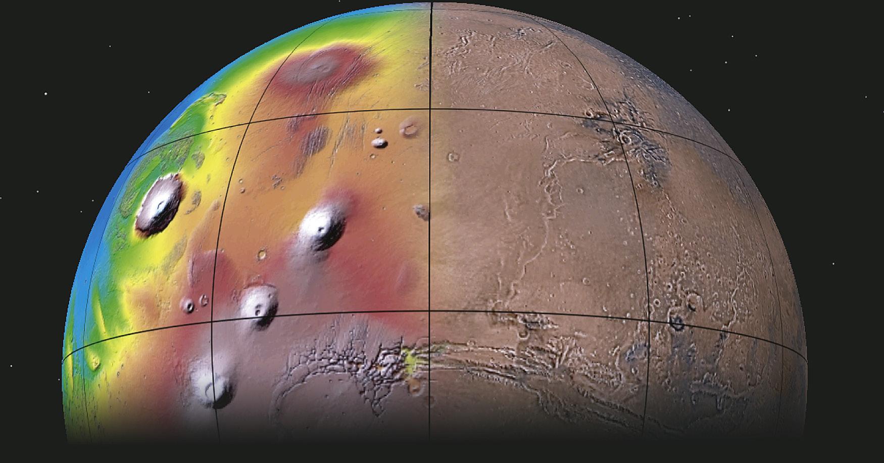
Northern part of the western hemisphere of Mars. Left half shows a color elevation, shaded-relief view highlighting the immense volcanic shields of the Tharsis rise. Right half shows a true-color view of the vast Valles Marineris and Kasei Valles canyon systems, which connect to the dark basin of Chryse Planitia at upper right. From Tanaka et al., 2014; Image data from National Aeronautics and Space Administration (NASA).
Introduction
Formal stratigraphic systems have been developed for the surfaces of Earth’s Moon, Mars, and Mercury (Fig. 2.1). The time scales are based on regional and global geologic mapping, which establishes relative ages of surfaces delineated by superposition, transaction, morphology, and other relations and features. Referent map units are used to define the commencement of events and periods for
definition of chronologic units. The following summary is mainly reproduced from Tanaka and Hartmann (2008, 2012).
Relative ages of these units in most cases can be confirmed using size–frequency distributions and superposed craters. For the Moon, the chronologic units and cratering record are constrained by radiometric ages measured from samples collected from the lunar surface. This allows a calibration of the areal density of craters versus age, which
2.1 (Continued)
Figure
Figure 2.1 Planetary time scale with selected major events. Thick dashed line separates the Venus and Mercury time scales. Diagram revised by G. Ogg from Tanaka and Hartmann (2012)
permits model ages to be measured from crater data for other lunar surface units. Model ages for other cratered planetary surfaces are constructed by two methods: (1) estimating relative cratering rates with Earth’s Moon and (2) estimating cratering rates directly based on surveys of the sizes and trajectories of asteroids and comets (e.g., Hartmann, 2005).
The Moon
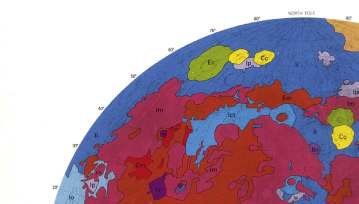
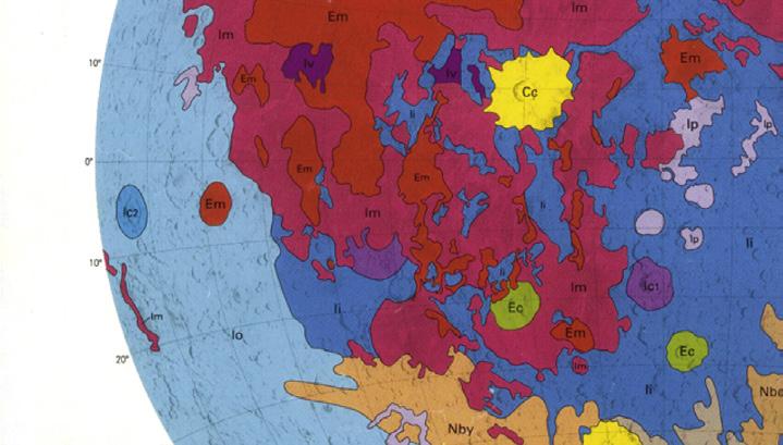
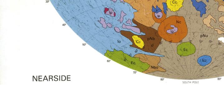
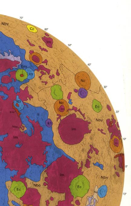
The first formal extraterrestrial stratigraphic system and chronology was developed for Earth’s Moon beginning in the 1960s, first based on geologic mapping using telescopic observations ( Shoemaker and Hackman, 1962). These early observations showed that the rugged lunar highlands are densely cratered, whereas the maria (Latin for “seas”) form relatively dark, smooth plains consisting of younger deposits that cover the floors of impact basins and intercrater plains. Resolving power of the lunar landscape improved greatly with the Lunar Orbiter spacecraft (Fig. 2.2), which permitted also the first mapping of the farside of the Moon. By the end of the decade and into the 1970s, manned and unmanned exploration of lunar sites by the Apollo and Luna missions brought return of samples. The majority of early exploration involved the lunar nearside (facing Earth), and the stratigraphic system and chronology follow geologic features and events primarily expressed on the nearside (see Fig. 2.3).
The cratering rate was initially very high; uncertain is whether the lunar cratering rate records a relatively brief period of catastrophic “Late Heavy Bombardment” in the inner solar system at ∼ 4.0 Ga, possibly spawned by perturbations in the orbits of the giant outer planets (e.g., Strom et al., 2005 ). Alternatively, the dense population of highland craters records the gradual trailing off of the accretionary period itself. Telescopic surveys of the numbers, sizes, and
orbits of asteroids indicate that they have been the prime contributor to the lunar cratering record.
The materials of the early crust and the emplacement of extensive lava flows that make up the lunar maria were dated by geologic inferences and by radiometric methods on samples returned by the Apollo missions (e.g., Wilhelms, 1987; Stöffler and Ryder, 2001 ). Attempts were also made to use the samples to date certain lunar basin-forming impacts and the large craters, Copernicus and Tycho. Two processes have mainly accomplished resurfacing: impacts and volcanism. Analogous to volcanism, impact heating can generate flowlike deposits of melted debris that can infill crater floors or terrains near crater rims. As on Earth, the broadest time intervals are designated “Periods” and their subdivisions are “Epochs” (if not meeting formal stratigraphic criteria, these unit categories are not capitalized).
From oldest to youngest, lunar chronologic units and their referent surface materials and events include:
1. pre-Nectarian period, earliest materials dating from solidification of the crust (a suite of anorthosite, norite, and troctolite) until just before formation of the Nectaris basin;
2. Nectarian Period, mainly impact melt and ejecta associated with Nectaris basin and later impact features;
3. Early Imbrian Epoch, consisting mostly of basin-related materials associated at the beginning with Imbrium basin and ending with Orientale basin;
4. Late Imbrian Epoch, characterized by mare basalts post-dating Orientale basin;
5. Eratosthenian Period, represented by dark, modified ejecta of Eratosthenes crater; and
6. Copernican Period, characterized by relatively fresh bright-rayed ejecta of Copernicus crater.
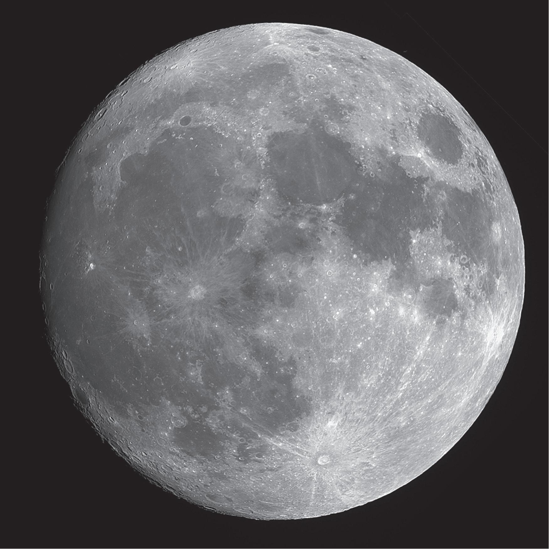
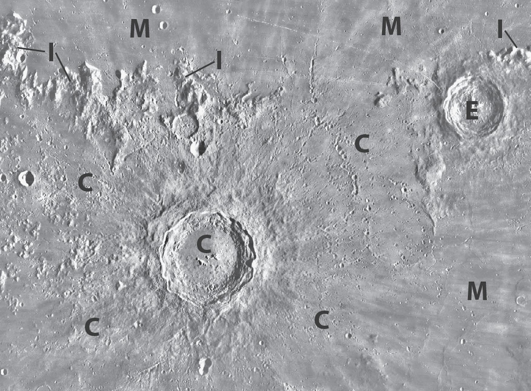
Figure 2.2 Lunar stratigraphy: (A) Photograph of the Moon. Provided by Gregory Terrance (Finger Lakes Instrumentation, Lima, New York; www.fli-cam.com)
Figure 2.2 (Continued) (B) Copernicus region of the Moon. Approximate location of this region is shown on a photograph of the Moon. Copernicus crater (C) is 93 km in diameter and centered at latitude (lat) 9.7°N, longitude (long) 20.1°W. Copernicus is representative of bright-rayed crater material formed during the lunar Copernican Period. Its ejecta and secondary craters overlie Eratosthenes crater (E), which is characteristic of relatively dark crater material of the Eratosthenian Period. In turn, Eratosthenes crater overlies relatively smooth mare materials (M) of the Late Imbrian Epoch. The oldest geologic unit in the scene is the rugged rim ejecta of Imbrium basin (I), which defines the base of the Early Imbrian Epoch (Lunar Orbiter IV image mosaic; north at top; illumination from right; courtesy of US Geological Survey (USGS) Astrogeology Team).
Mars
The Red Planet has a geologic character similar to the Moon, with vast expanses of cratered terrain and lava plains, but with the important addition of features resulting from the activity of wind and water over time. This results in a geologically complex surface history; geologic mapping has assisted in unraveling it, following the approaches developed for studies of
the Moon (Fig. 2.4). Beginning in the 1970s with the Mariner 9 and Viking spacecraft, and continuing with a flotilla of additional orbiters and landers beginning in the 1990s, Mars has become a highly investigated planet. Geologic mapping led to characterization of periods and epochs as on the Moon (e.g., reviews in Tanaka, 1986; Kallenbach et al., 2001; Nimmo and Tanaka, 2005; Tanaka et al., 2014 ) (Fig. 2.1).
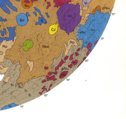
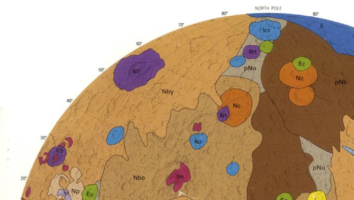
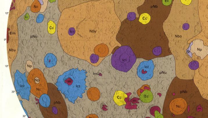
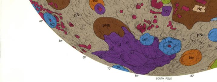
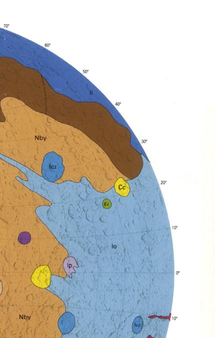
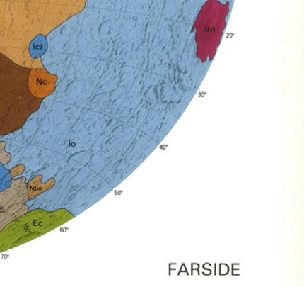
Figure 2.3 Generalized geologic map of Earth’s Moon.
GEOLOGIC UNITS
A polar layered deposits
EA Vastitas Borealis unit
LH-LA volcanic materials
H materials
LN-EH knobby materials
LN-EH materials
N-EH volcanic materials
N materials
EN massif material
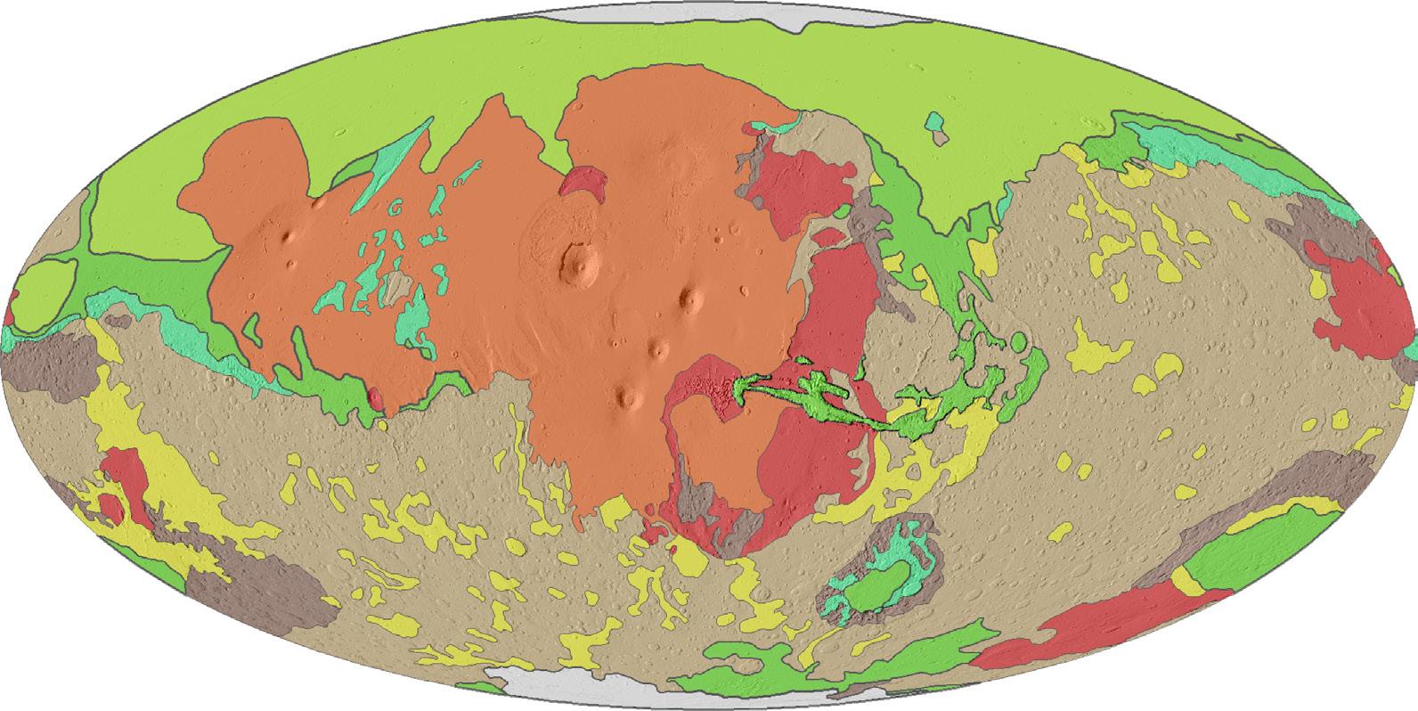
Figure 2.4 Global geologic map of Mars. Generalized geologic map of Mars showing distribution of major material types and their ages. Chronologic unit abbreviations: N, Noachian; H, Hesperian; A, Amazonian; E, Early; L, Late. (Adapted from Nimmo and Tanaka (2005) ) Terrain names shown without descriptor terms. Mollweide projection, using east longitudes, centered on 260°E, Mars Orbiter Laser Altimeter (MOLA) shaded-relief base illuminated from the East. On Mars, 1° latitude = 59 km.
The pre-Noachian period represents the age of the early crust and is not represented in known outcrops, but a Martian meteorite, ALH84001, was crystallized at ∼4.5 Ga.
Heavily cratered terrains formed during the Noachian Period. These include large impact basins of the Early Noachian Epoch, vast cratered plains of the Middle Noachian, and intercrater plains resurfaced by fluvial and possibly volcanic deposition during the Late Noachian when the atmosphere apparently was thicker and perhaps warmer and heat flow was higher.
Hesperian Period rocks are much less cratered and record waning fluvial activity but
extensive volcanism, particularly during the Early Hesperian Epoch. Mars Express and Mars Reconnaissance Orbiter data indicate that clay minerals occur in some Noachian strata, whereas hydrated sulfates are mostly in Hesperian rocks. A thick permafrost zone developed as the surface cooled, and much of the fluvial activity during the Late Hesperian Epoch occurred as catastrophic flood outbursts through this frozen zone, perhaps initiated by magmatic activity.
The Amazonian Period began with expansive resurfacing of the northern lowlands, perhaps by sedimentation within a large body of water. Much lower levels of volcanism
Tyrrhena
Cimmeri a
Australe
and fluvial discharges, coupled with aeolian deposition and erosion continued into the Middle and Late Amazonian Epochs. Continued weathering has led to iron oxidation of surface materials.
The polar plateaus, covered by bright deposits of residual ice as well as seasonally waxing and waning meter-thick CO2 frost, are among the youngest features on the planet. Ice-rich mantles and glacial-like deposits at middle and equatorial latitudes signal climate oscillations in the relatively recent geologic record.
The NASA rover, Curiosity, is investigating Gale Crater, which formed toward the end of the Noachian Period (Le Deit et al., 2012). This crater was partly filled by fluvial, deltaic, and lacustrine sediments over a few hundred million years during the early part of the Hesperian Period. These deposits were partially exhumed by wind erosion during the middle Hesperian (ca. 3.3 to 3.1 billion years ago) to form the massive Aeolis Mons (Mount Sharp) of cyclic sediment deposits up to 5-km thick and 6000 km2 in area within the Gale crater (e.g., Grotzinger et al., 2015). There has been only very slow eolian erosion since the middle Hesperian.
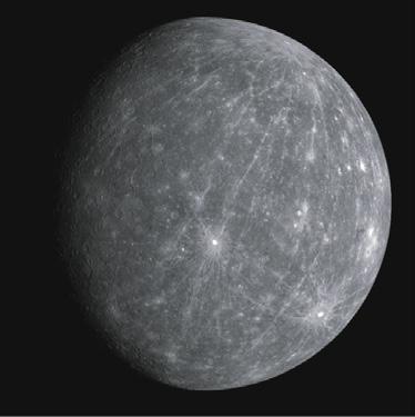
Mercury
The innermost planet was partly imaged by flybys of the Mariner 10 spacecraft in 1974 and 1975, enabling stratigraphic studies that reveal a remarkably similar surface history to that of Earth’s Moon (e.g., Spudis and Guest, 1988). Consequently, a Mercurian chronology was developed based on impact basins and craters that may have similar histories to comparable lunar features (Fig. 2.1).
Thus, five major periods have been proposed that correspond to those of the Moon, as follows:
pre-Tolstojan (equivalent to the lunar pre-Nectarian)
Tolstojan (Nectarian)
Calorian (Imbrian)
Mansurian (Eratosthenian)
Kuiperian (Copernican)
Absolute ages for these periods are much more uncertain than for the Moon and Mars.
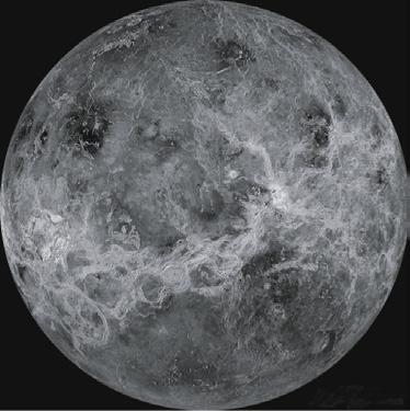
Venus
The Venusian surface has been investigated extensively with orbiters and landers, most recently by the Magellan orbiter with its mapping radar in the 1990s. Impact crater densities are low. Statistics of nearly 1000 impact craters on its surface indicate that Venus has an average surface age of hundreds of millions of years. Despite its spectacular volcanic surface dotted with thousands of volcanoes and broad fields of lava flows, all of which has been tectonically disrupted to varying degrees, the details of the global geologic evolution of this Earth’s twin planet in size are not well constrained. Possibilities range from local to regional events driven by mantle plumes to global volcanic and tectonic evolution driven by atmospheric greenhouse-heating effects on Venusian climate (e.g., Bougher et al., 1997).
Other solar system bodies
The solid surfaces of asteroids and satellites of Jupiter, Saturn, Uranus, and Neptune show varying degrees of cratering that reflect surface ages (e.g., Schenk et al., 2004). Although asteroids are commonly saturated with craters, indicating their primordial origin, some asteroids, comet nuclei, and other bodies demonstrate later resurfacing as their rocky or icy crusts evolved. Dating these surfaces relies on inferences of the populations of projectiles across time and space. Absolute dates are very poorly constrained. Complications in estimates of cratering rates include the relative importance of asteroids in the
inner solar system versus that of comets and other icy materials of the Kuiper Belt.
Selected publications and websites
Cited publications
Bougher, S.W., Hunten, D.M., Phillips, R.J., 1997. Venus II: Geology, Geophysics, Atmosphere, and Solar Wind Environment. The University of Arizona Press, Tucson. 1362 pp.
Grotzinger, et al., 2015. Deposition, exhumation, and paleoclimate of an ancient lake deposit, Gale crater, Mars (47 authors total) Science 350: 177. http:// dx.doi.org/10.1126/science.aac7575 summary; full version (12 pp.) at.
Hartmann, W.K., 2005. Martian cratering 8: isochron refinement and the chronology of Mars. Icarus 174: 294–320.
Kallenbach, R., Geiss, J., Hartmann, W.K., 2001. Chronology and Evolution of Mars. Kluwer Academic Publishers, Dordrecht. 498 pp.
Le Deit, L., Hauber, E., Fueten, F., Mangold, N., Pondrelli, M., Rossi, A., Jaumann, R., 2012. Model age of Gale Crater and origin of its layered deposits. In: Third International Conference on Early Mars: Geologic and Hydrological Evolution, Physical and Chemical Environments, and the Implications for Life (Lake Tahoe, Nevada, 21–25 May 2012): 7045.pdf http:// www.lpi.usra.edu/meetings/earlymars2012/ pdf/7045.pdf
Nimmo, F., Tanaka, K., 2005. Early crustal evolution of Mars. Annual Review of Earth and Planetary Sciences 33: 133–161.
Schenk, P.M., Chapman, C.R., ZahnIe, K., Moore, J.M., 2004. Ages and interiors: the cratering record of the Galilean satellites. In: Bagenal, F., Dowling, T.E., McKinnon, W.B. (Eds.), Jupiter: The Planet, Satellites and Magnetosphere. Cambridge University Press, Cambridge, pp. 427–456.
Shoemaker, E.M., Hackman, R.J., 1962. Stratigraphic basis for a lunar time scale. In: Kopal, Z., Mikhailov, Z.K. (Eds.), The Moon. Academic Press, London, pp. 289–300.
Spudis, P.D., Guest, J.E., 1988. Stratigraphy and geologic history of Mercury. In: Vilas, F., Chapman, C.R., Matthews, M.S. (Eds.), Mercury. The University of Arizona Press, Tucson, pp. 118–164.
Stöffler, D., Ryder, G., 2001. Stratigraphy and isotope ages of lunar geologic units: chronological standards for the inner solar system. Space Science Reviews 96: 9–54.
Strom, R.G., Malhotra, R., Ito, T., Yoshida, F., Kring, D.A., 2005. The origin of planetary impactors in the inner solar system. Science 309: 1847–1850.
Tanaka, K.L., 1986. The stratigraphy of Mars. Proceedings of the Lunar and Planetary Science Conference, 17, Part 1. Journal of Geophysical Research 91: E139–E158.
Tanaka, K.L., Hartmann, W.K., 2008. 2 planetary time scale. In: Ogg, J.G., Ogg, G., Gradstein, F.M. (Eds.), The Concise Geologic Time Scale. Cambridge University Press, pp. 13–22.
Tanaka, K.L., Hartmann, W.K., 2012. The planetary time scale. In: Gradstein, F.M., Ogg, J.G., Schmitz, M., Ogg, G., (Coordinators). The Geologic Time Scale 2012 Elsevier Publisher, pp. 275–298. (An overview on the geologic history of all inner planets, Earth’s Moon, and briefly on the moons of Mars and Jupiter.).
Wilhelms, D.E., 1987. The geologic history of the Moon. U.S. Geological Survey Professional Paper 1348 302 pp., 12 plates.
Selected further reading
Basaltic Volcanism Study Project, 1981. Basaltic Volcanism on the Terrestrial Planets. Houston: Lunar and Planetary Institute, Houston. 1286 pp. Melosh, H.J., 2011. Planetary Surface Processes Cambridge University Press. 500 pp.
Websites (selected)
US Geological Survey Astrogeology Research Program astrogeology.usgs.gov/, especially: Astropedia: astrogeology.usgs.gov/search/. Solar System Exploration (NASA) solarsystem.nasa. gov.
Welcome to the Planets (JPL, NASA) pds.jpl.nasa.gov/ planets/.
Mars Exploration Program (NASA) marsprogram.jpl. nasa.gov/.
Wikipedia Lunar Geologic Timescale en.wikipedia. org/wiki/Lunar_geologic_time_scale; and Geologic history or Mars: https://en.wikipedia.org/wiki/ Geological_history_of_Mars
PRECAMBRIAN
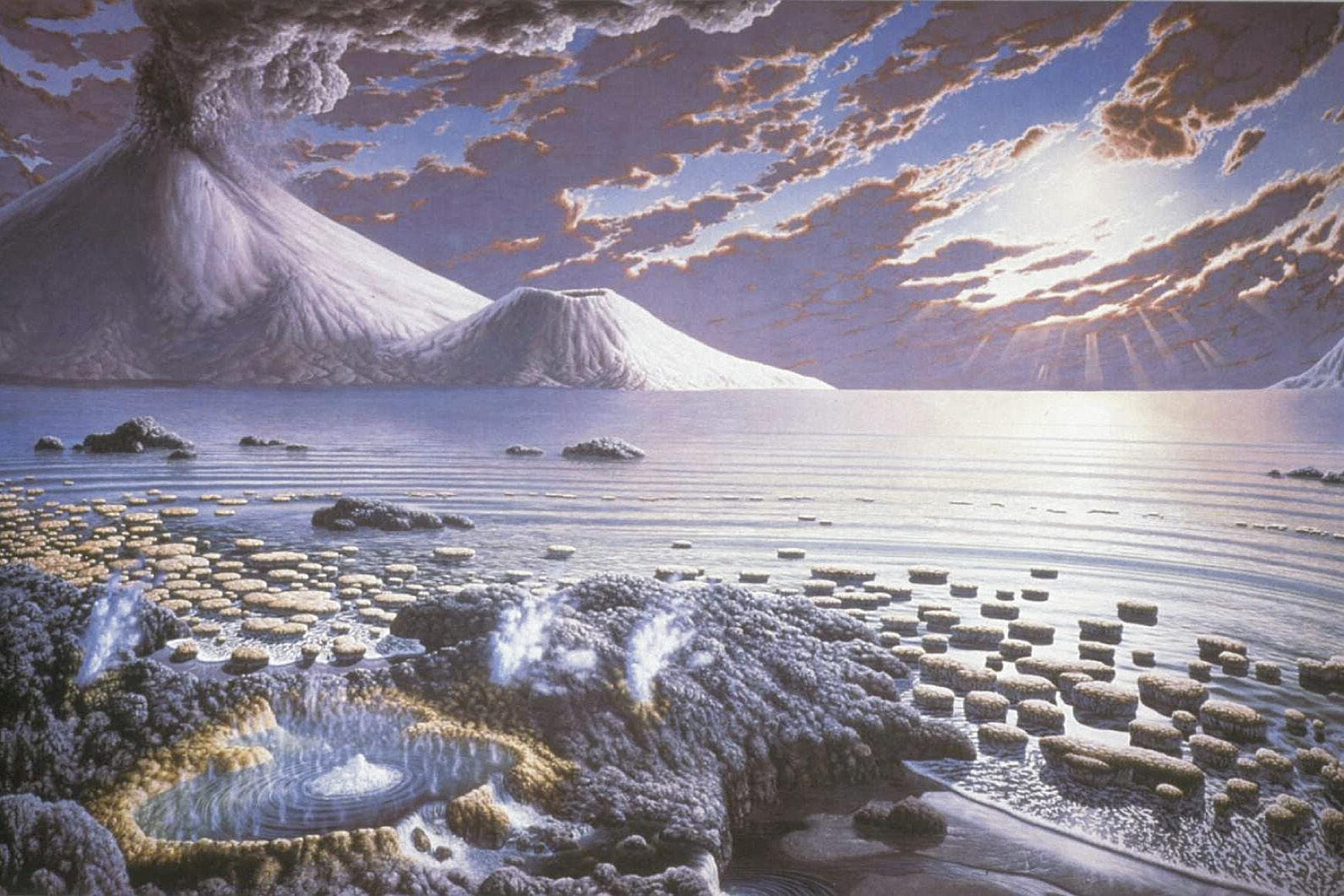
The Archean World. Courtesy of the Smithsonian Institution. Painting by Peter Sawyer. [http://ocean.si.edu/slideshow/ ocean-throughout-geologic-time-image-gallery]
Status of international subdivisions
The first 4 billion years of Earth’s history consist of the Hadean, Archean, and Proterozoic eons. The Precambrian simply refers to the time interval and all rocks that formed prior to the beginning of the Cambrian Period (base of Phanerozoic Eon) at 541 Ma.
The interval with no preserved rock record from the formation of the Earth at 4.567 to ca. 4 Ga is named the “Hadean” Eon, a term derived from Greek for “unseen place” and also referring to the mythical Hades land of the dead (Subcommission on Precambrian Stratigraphy, 2014). The Hadean is followed at ca. 4 Ga by the Archean (from the Greek word meaning “beginning/origin”) and at ca. 2.5 Ga by the Proterozoic (from Greek for “earlier life”) (Fig. 3.1).
A Concise Geologic Time Scale. http://dx.doi.org/10.1016/B978-0-444-59467-9.00003-0
Long period of stable one-celled-life ecosystems in apparently constant environments
Supercontinent Rodinia (~1300 to 900 Ma)
Supercontinent Columbia/Nuna formation, then break-up
Increased burial of organic carbon (”L-J” 13C positive excursion)
Oxygen begins to accumulate in atmosphere; major glaciations
Oxygen levels rise in oceans causing banded-iron formations
Sedimentary basins on stable or growing continents
Growth of nuclei of continents
Earliest preserved sedimentary rocks and chemical traces of life
Oldest preserved pieces of continental crust
Rapid crust formation & recycling; heavy meteorite bombardment
Earliest Life (Prokaryotes, simple-celled) evolved?
Accretion of Earth; then giant Moon-forming impact event
Figure 3.1 The current Precambrian time scale. The current Precambrian eons, eras, and periods, from the International Commission on Stratigraphy, based on Plumb and James (1986) and Plumb (1991). Note that Precambrian is not a formal time scale unit and that all divisions of the Precambrian are chronometric (fixed dates at base). Exceptions are the Cryogenian and the Ediacaran. The base of the Cryogenian Period was initially set at 850 Ma (Plumb, 1991), but was revised in 2014/2015 to the ca. 720 Ma date of the onset of the first global glaciation—the criteria for placement of a future GSSP. The base of the Ediacaran is a chronostratigraphic GSSP at the termination of the last Cryogenian glaciation dated as 635 Ma (see next chapter). Only era divisions are shown for the Phanerozoic Eon. In the years since these Precambrian divisions were standardized in 1990, our dating of major events and cycles in Precambrian geologic history have indicated that the current Global Standard Stratigraphic Ages (GSSAs) do not adequately convey this history.
Although microbial life existed throughout the Archean and Proterozoic, the lack of a diverse and well-preserved fossil record prior to the late Ediacaran, coupled with uncertainties in geochemical or other stratigraphic means of correlations, is a challenge to establish a formal chronostratigraphic scale. Radioisotopic dating was the main method for correlating the Precambrian geologic records; therefore, the Subcommission on Precambrian Stratigraphy adopted the use of chronometric GSSAs for the international subdivisions and standardization of interregional geological maps (Plumb and James, 1986; Plumb, 1991).
The Archean Eon is subdivided into four eras (rounded to the nearest 100-myr boundaries), and the Proterozoic into three eras and 10 periods (the first eight of which are rounded to the nearest 50-myr boundaries). The two youngest periods, Cryogenian (ca. 720 Ma to 635 Ma) with its major glaciations and the Ediacaran (635–541 Ma) with metazoan life forms, are summarized in the next chapter. The dates for these GSSA boundaries (and the poetic names for the Proterozoic periods) were selected to delimit major events in tectonics, surface conditions, and sedimentation as known in 1990 ( Table 3.1).
Summary of Precambrian trends and events, and a potential revised time scale
Since 1990, our knowledge and dating of the development of Earth’s tectonic cycles, crustal features, atmosphere and ocean composition, geochemical trends and excursions, major volcanic and impact events, and stages in evolution of life through the Precambrian has vastly increased. Some major trends are displayed in Fig. 3.2.
The shortcomings of the current rounded dates for the chronometric subdivisions of Precambrian time are: (1) a lack of ties of
stratigraphic boundaries to the actual rock record, (2) the current divisions do not adequately convey the major events in the fascinating history of our planet, and (3) severe diachroneity of global tectonic events. Hence, major research efforts are underway by the Subcommission on Precambrian Stratigraphy to replace the current GSSA chronometric scheme to one that is more naturalistic with GSSPs. In GTS2012, members of the Subcommission on Precambrian Stratigraphy under the leadership of Martin van Kranendonk, suggested a possible stratigraphic scheme (revised from Bleeker, 2004) that is principally based on sedimentological, geochemical, geotectonic, and biological events recorded in the rock record with potential “golden spikes” ( Van Kranendonk et al., 2012) (Figs. 3.2 and 3.3).
The following summary is largely based on the extensive Precambrian synthesis by Van Kranendonk et al. (2012) and Van Kranendonk (2014).
Hadean
The oldest solid materials in the solar system, therefore the oldest rocks that would have been incorporated in the accretion of planet Earth, are considered calcium–aluminum-rich aggregates in chondritic meteorites that are dated as 4.567 Ga; and that date is assigned as the beginning of the Hadean Eon. After the giant Moon-forming impact at ca. 4.5 Ga, the sphere of molten silicate material cooled and differentiated into the core and mantle. The oldest preserved mineral crystals from cooling of magma on Earth are zircons dated 4.4 Ga that were later recycled into weakly metamorphosed sandstone in the Jack Hills of the Yilgarn Craton of Western Australia. One of these zircons has been reanalyzed by high-resolution mapping of radiogenic isotopes to yield a precise 4.374 ± 0.006 Ga date ( Valley et al., 2014; reviewed by Bowring, 2014). This early crust was largely destroyed during the Late Heavy
Table
3.1 Nomenclature for periods of Proterozoic Eon in the current International Commission on Stratigraphy (ICS) geologic time-scale with their intended characteristics
Period name Base (Ma)
Ediacaran ∼635
Cryogenian ∼720
Tonian 1000
Stenian 1200
Ectasian 1400
Calymmian 1600
Statherian 1800
Orosirian 2050
Rhyacian 2300
Siderian 2500
Derivation and geological process
Ediacara = from Australian Aboriginal term for place near water
“Earliest metazoan life”
GSSP in Australia coincides with termination of glaciations and a pronounced carbonisotope excursion
Cryos = ice; Genesis = birth
“Global glaciation”
Glacial deposits, which typify the late Proterozoic, are most abundant during this interval. Base, formerly at 850 Ma, was re-defined in 2014/2015 as onset of the first global glaciation.
Tonas = stretch
Further major platform cover expansion (e.g., Upper Riphean, Russia.; Qingbaikou, China; basins of northwest Africa), following final cratonization of polymetamorphic mobile belts.
Stenos = narrow
“Narrow belts of intense metamorphism & deformation”
Narrow polymetamorphic belts, characteristic of the mid-Proterozoic, separated the abundant platforms and were orogenically active at about this time (e.g., Grenville, Central Australia).
Ectasis = extension
“Continued expansion of platform covers”
Platforms continue to be prominent components of most shields.
Calymma = cover
“Platform covers”
Characterized by expansion of existing platform covers, or by new platforms on recently cratonized basement (e.g., Riphean of Russia).
Statheros = stable, firm
“Stabilization of cratons; Cratonization”
This period is characterized on most continents by either new platforms (e.g., North China, north Australia) or final cratonization of fold belts (e.g., Baltic Shield, north America).
Orosira = mountain range
“Global orogenic period”
The interval between about 1900 and 1850 Ma was an episode of orogeny on virtually all continents.
Rhyax = stream of lava
“Injection of layered complexes”
The Bushveld Complex (and similar layered intrusions) is an outstanding event of this time.
Sideros = iron
“Banded iron formations”(BIFs)
The earliest Proterozoic is widely recognized for an abundance of BIFs, which peaked just after the Archean–Proterozoic boundary. Modified from Plumb (1991)
Bombardment resurfacing of the inner solar system planets and Moon (ca. 4.1 to 3.85 Ga).
The accretion of planet Earth, partial differentiation of its core–mantle, and the formation of the Moon from the ejected residual from a massive impact with Earth all occurred during the “Chaotian” interval between these two dates ( Van Kranendonk et al., 2012).
Archean
The oldest surviving rocks that have been dated, the Acasta Gneiss Complex of the Slave Craton in Canada, at 4.03 Ga (Bowring and Williams, 1999), form the base of the Archean. The oldest sedimentary rocks with preserved primary features are in the Isua supracrustal belt of the North Atlantic Craton, western Greenland with an age of 3.81 Ga.
The oldest well-preserved structures formed by life are stromatolites from ancient microbial mats in the Dresser Formation of the Warrawoona Group from the humorously named “North Pole” dome region of the Pilbara Craton of Western Australia, dated at ca. 3.481 ± 0.002 Ga (e.g., Van Kranendonk et al., 2008). The oldest known intertidal shoreline deposit, the Strelley Pool Formation of Western Australia, dated at ca. 3.43 Ga, contains stromatolites and candidates for organic microfossils preserved in episodic silica cementation (Brasier et al., 2015). The origins of life itself are not known and remain a major challenge facing science.
Van Kranendonk et al. (2012) suggest using this suite of the oldest rock, the oldest well-preserved sediment, and the oldest biostructure as chronostratigraphic boundaries to delimit the Acastan and the Isuan periods within a Paleoarchean Era.
Basins formed within the growing cratons during the Mesoarchean Era, and this Era could be subdivided with a GSSP at the base of ca. 3 Ga quartz-rich sandstone in a platform setting. Dating of crustal rocks indicate that there was another widespread growth period
of continental crust beginning at ca. 2.78 until 2.63 Ga (e.g., O’Neill et al., 2015) (Fig. 3.2).
The expansion of photosynthetic life in these basins removed carbon dioxide in the form of stromatolite carbonates. However, carbon preserved in kerogen in these stromatolites during the interval from ca. 2.7 to 2.5 Ga has highly negative δ13Corg values (down to −61 per mille), indicative of a dominance of 12C-enriched products from methaneproducing organisms or other methanogenesis process. The photosynthesis activity and carbon burial also increased the influx and concentration of oxygen waste products in the atmosphere and oceans. The oxygen dissolving into the marine waters caused precipitation of iron oxides, which resulted in a unique episode of extensive banded iron formations (BIF) beginning at ca. 2.6 Ga. The onsets of these relatively rapid and easily correlated global changes are options for redefining and subdividing the Neoarchean Era into an earlier “Methanian Period” before the methane-producing microbes were inhibited by the rising oxygen levels, followed by a “Siderian Period” for the main episode of BIF deposition as characterized by those in the Hamersley Basin of Western Australia ( Van Kranendonk et al., 2012) (Figs. 3.2 and 3.3).
Proterozoic
The rising oxygen levels, increased weathering rates, and burial of carbon led to major changes in the Earth system beginning at ca. 2.42 Ga—just after the traditional placement for the Archean/Proterozoic boundary at 2.5 Ga. Extensive removal of atmospheric carbon dioxide contributed to the near-global “Huronian” glaciations during ca. 2.4–2.25 Ga (e.g., review by Tang and Chen, 2013). When this “Snowball Earth” episode ended, it was a different world. In the oxygenated oceans, the complex-celled eukaryotic life forms with aerobic metabolism appeared and thrived, later evolving into Phanerozoic animals.